Preprint no. NJU-INP 073/23, USTC-ICTS/PCFT-23-13
Polarised parton distribution functions and proton spin

Abstract

Supposing there exists an effective charge which defines an evolution scheme for both unpolarised and polarised parton distribution functions (DFs) that is all-orders exact and using Ansätze for hadron-scale proton polarised valence quark DFs, constrained by flavour-separated axial charges and insights from perturbative quantum chromodynamics, predictions are delivered for all proton polarised DFs at the scale $\zeta_{\rm C}^{2}=3\,$GeV². The pointwise behaviour of the predicted DFs and, consequently, their moments, compare favourably with results inferred from data. Notably, flavour-separated singlet polarised DFs are small. On the other hand, the polarised gluon DF, $\Delta G(x;\zeta_{\rm C})$, is large and positive. Using our result, we predict $\int_{0.05}^{1}\,dx\,\Delta G(x;\zeta_{\rm C})=0.214(4)$ and that experimental measurements of the proton flavour-singlet axial charge should return $a_{0}^{\rm E}(\zeta_{\rm C})=0.35(2)$.

1 Introduction

The proton is Nature’s most fundamental bound-state. In isolation, it is stable; at least, the lower bound on its lifetime is many orders-of-magnitude greater than the $\sim 14$-billion-year age of the Universe. Further, the proton is characterised by two basic Poincaré invariant quantities: mass squared, $m_{p}^{2}$; and total angular momentum squared, $J^{2}=J(J+1)=3/4$. One can also include parity, $P=+1$, in which case the proton is identified as a $J^{P}=\tfrac{1}{2}^{+}$ state.

Contemporary theory posits that the proton is constituted from three valence quarks: $u+u+d$, which interact according to rules laid down by the Lagrangian density of quantum chromodynamics (QCD). Itself, QCD is a Poincaré-invariant quantum non-Abelian gauge field theory. It is worth stressing that $P$ is a Poincaré invariant quantum number. On the other hand, every separation of $J$ into a sum of orbital angular momentum and spin, $L+S$, is observer dependent. Hence, there is no relation between $P$ and $L$ in QCD and no objective (Poincaré-invariant) meaning for $L$, $S$ separately [1].

Assuming isospin symmetry, viz. that $u$ and $d$ quarks are mass-degenerate, then the wave function of the $J^{P}=\tfrac{1}{2}^{+}$ proton is a Poincaré-covariant four-component spinor whose complete form involves 128 distinct scalar (Poincaré-invariant) functions [2, 3]. It follows that in any observer-dependent reference frame, this wave function contains $\mathsf{S}$-, $\mathsf{P}$- and $\mathsf{D}$-wave orbital angular momentum components. The character of the angular momentum described by these components depends on the degrees-of-freedom (dof) used to solve the proton bound state problem. Typically, those dof change with the resolving scale of any probe used to measure a proton property. Evidently in QCD, there is no scale at which the proton $J=\tfrac{1}{2}$ can simply be the sum of the spins of the valence dof [4]. Analogous statements may be made about $m_{p}^{2}$; namely, the manner by which the proton mass is shared amongst its constituents depends upon the choices of variables and frame made when solving the bound-state problem. Either or both of these may depend on the resolving scale used to specify the problem.

These remarks make plain that there is no objective meaning to any separation of the proton’s $J=\tfrac{1}{2}$ into subcomponents of any kind. Such a separation is contextual, acquiring significance only once choices of variables and frame are made. A useful frame is that reached after projection of Poincaré-covariant wave functions onto the light-front because the wave functions obtained thereby are the probability amplitudes connected with parton distribution functions (DFs) [5, 6, 7].

Issues related to the choice of variables are more complex. Herein we adopt a perspective characteristic of continuum Schwinger function methods (CSMs) [8, 9]. Namely, at the hadron scale, $\zeta_{\cal H}<m_{p}$, QCD bound-state problems are most efficiently solved in terms of dressed-parton dof: dressed-gluons and -quarks, each of which possesses a momentum-dependent mass. This approach is firmly founded in QCD theory and has widely been used with phenomenological success – see, e.g., Refs. [10, 11, 12, 13, 14, 15, 16, 17] for discussions of both facets. Notably, $\zeta_{\cal H}$ is the scale at which all properties of a given hadron are carried by its valence quasiparticle dof [18, 19, 20].

2 Proton Faddeev equation

A key feature of strong interactions is emergent hadron mass (EHM), i.e., absent Higgs boson couplings into QCD, the dynamical generation of a nuclear-scale mass for the proton, $m_{p}\approx 1\,$GeV, concomitant with the formation of massless pseudoscalar Nambu-Goldstone bosons [21]. As a corollary of EHM, any quark+antiquark interaction that delivers a good description of meson properties also generates nonpointlike quark+quark (diquark) correlations in multiquark systems [22]. A discussion of the empirical evidence for such diquark correlations is presented elsewhere [23]. Profiting from the emergence of diquarks, a fully-interacting dressed-quark+nonpointlike-diquark approximation to the proton bound-state equation was introduced in Refs. [24, 25, 26]. It has proven effective in describing proton properties – see, e.g., Ref. [23, Sec. 2.2]. A benefit of working with this simplification is that at most 16 (instead of 128) scalar functions are necessary to fully express the Poincaré-covariant proton wave function.

Table 1: Gegenbauer coefficients that define the hadron-scale valence quark DFs in Eq. (1). Each entry should be divided by $10^{3}$.

$a_{n}^{\mathpzc u}$
1	2	3	4	5
$403$	$112$	$7.31$	$-10.4$	$-4.90\$
6	7	8	9	10
$-0.0474$	$1.15$	$0.828$	$0.334$	$0.0635$
$a_{n}^{\mathpzc d}$
1	2	3	4	5
$482$	$161$	$20.8$	$-11.5$	$-7.11\$
6	7	8	9	10
$-0.430$	$1.50$	$1.03$	$0.349$	$0.0543$

In proceeding, the following hadron-scale quark+diquark Faddeev equation predictions are important.

1. The proton contains both isoscalar-scalar (SC) and isovector-axialvector (AV) diquark correlations, with the AV correlations being responsible for $\approx 35$% of the wave function canonical normalisation [27].

2. In the rest frame, the proton quark+diquark Faddeev wave function contains $\mathsf{S}$-, $\mathsf{P}$- and $\mathsf{D}$-wave orbital angular momentum components [28, Fig. 3a].

3. Calculated unpolarised valence quark DFs in a proton with the preceding two features are reliably interpolated by a finite sum of Gegenbauer polynomials [29]:

   $${\mathpzc q}(x;\zeta_{\cal H})=n_{\mathpzc q}140x^{3}(1-x)^{3}\left[1+\sum_{n=1}^{10}a_{n}^{\mathpzc q}C_{n}^{7/2}(1-2x)\right]\,,$$ (1)

   $n_{\mathpzc u}=2n_{\mathpzc d}=2$, where the coefficients are listed in Table 1.

4. In agreement with experiment [30], the predicted proton axial charge is $g_{A}=1.25(3)$ [31], where the uncertainty reflects that on the masses of the SC and AV diquarks: $m_{\rm SC}\approx 0.8\,$GeV; $m_{\rm AV}\approx 0.9\,$GeV. Furthermore, the $u$ quark fraction of the axial charge is $g_{A}^{u}/g_{A}=0.76(1)$; that of the $d$ quark is $g_{A}^{d}/g_{A}=-0.24(1)$; and $g_{A}^{d}/g_{A}^{u}=-0.32(2)$.

5. The singlet axial charge of the proton is [14, Sec. 9]:

   $$a_{0}=0.65(2)\,.$$ (2)

   At $\zeta_{\cal H}$, the remainder of the proton spin is stored in quark+diquark orbital angular momentum. Similar statements hold even if the quark+quark interaction is momentum-independent [32].

3 Polarised valence quark distribution functions at $\zeta_{\cal H}$

To deliver a Faddeev equation based prediction for the hadron-scale polarised valence quark DFs, one must generalise the methods used for the unpolarised DFs in Ref. [29], centred on the vector current, to the axial current case. A symmetry-preserving axial current appropriate for use with a solution of the quark+diquark Faddeev equation has recently been derived [33, 34]; but some time will be required before it can be adapted to the calculation of polarised valence quark DFs.

Table 2: Referring to Eq. (3), central values of the mapping parameters, $\gamma^{\mathpzc q}$, that reproduce the given quark’s contribution to the proton axial charge.

$i$	1	2	3	4
$\gamma_{i}^{\mathpzc u}$	$0.350$	$0.621$	$0.575$	$0.853\$
$\gamma_{i}^{\mathpzc d}$	$1.47\phantom{0}$	$1.26\phantom{1}$	$2.62\phantom{5}$	$1.60\phantom{3}\$

Meanwhile, we employ a phenomenological approach to the problem, kindred to those used, e.g., in Refs. [35, 36], and exploit constraints suggested by analyses in perturbative QCD [37] to develop simple Ansätze for the polarised DFs. It is worth enumerating the constraints we impose.

1. At low-$x$, there is no correlation between the helicity of the struck quark and that of the parent proton; so, the polarised:unpolarised ratio of DFs must vanish: as $x\to 0$, $\Delta{\mathpzc q}(x;\zeta_{\cal H})/{\mathpzc q}(x;\zeta_{\cal H})\to 0$. Drawing on Regge phenomenology, we implement this by writing $\Delta{\mathpzc q}(x;\zeta_{\cal H})\propto x^{\delta\alpha_{R}}{\mathpzc q}(x;\zeta_{\cal H})$, where $\delta\alpha_{R}=\tfrac{1}{2}$ is the difference between the intercepts of the vector and axialvector meson Regge trajectories [38].

2. At high-$x$, the polarised and unpolarised valence quark distributions possess the same power-law behaviour, viz. $\Delta{\mathpzc q}(x)/{\mathpzc q}(x)\to{\rm constant}\neq 0$ as $x\to 1$.

These constraints are implemented using four distinct mappings: $\Delta{\mathpzc q}(x;\zeta_{\cal H})\!=\!{\mathpzc s}_{\mathpzc q}{\mathpzc r}_{i}(x,\gamma_{i}^{\mathpzc q}){\mathpzc q}(x;\zeta_{\cal H})$, with ${\mathpzc s}_{\mathpzc u}\!=\!1\!=\!-{\mathpzc s}_{\mathpzc d}$,

$$r_{1}(x,\gamma) =\sqrt{x}/[1+\gamma\sqrt{x}]\,, r_{2}(x,\gamma) =\sqrt{x}/[\gamma+\sqrt{x}]\,,$$ (3a)

$$r_{3}(x,\gamma) =\sqrt{x}/[1+\gamma x]\,, r_{4}(x,\gamma) =\sqrt{x}/[\gamma+x]\,.$$ (3b)

In each case, $\gamma_{i}^{\mathpzc q}$ is fixed by requiring $\int_{0}^{1}dx\,\Delta{\mathpzc q}(x;\zeta_{\cal H})=g_{A}^{\mathpzc q}$. Referring to Sec. 2-item (iv), this leads to the values listed in Table 2.

Our Ansätze for the hadron-scale polarised valence quark DFs are drawn in Fig. 1, wherein they are compared with the kindred unpolarised DFs calculated in Ref. [29] – reproduced by Eq. (1) with the coefficients in Table 1.

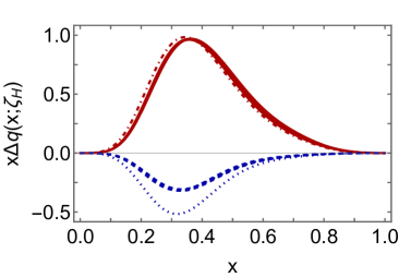
Figure 1: Hadron scale polarised valence quark distributions: solid red curves – $\mathpzc u$ quark; and dashed blue curves – $\mathpzc d$ quark. In each case, there are five curves, viz. the four produced by the mapping functions in Eq. (3), with the coefficient values in Table 2, and the average of these curves. Context is provided by the unpolarised valence quark distributions: $x{\mathpzc u}(x;\zeta_{\cal H})/2$ – dot-dashed red curve; and $[-x{\mathpzc d}(x;\zeta_{\cal H})/2]$ – dotted blue curve.

	herein	Faddeev	SC only	SU$(4)$	pQCD
$\rule{0.0pt}{12.91663pt}\frac{F_{2}^{n}}{F_{2}^{p}}$	$\phantom{-}0.45(5)$	$\phantom{-}0.49$	$\frac{1}{4}$	$\phantom{-}\frac{2}{3}$	$\frac{3}{7}$
$\frac{d}{u}$	$\phantom{-}0.23(6)$	$\phantom{-}0.28$	0	$\phantom{-}\frac{1}{2}$	$\frac{1}{5}$
$\frac{\Delta d}{\Delta u}$	$-0.14(3)$	$-0.11$	0	$-\frac{1}{4}$	$\frac{1}{5}$
$\frac{\Delta u}{u}$	$\phantom{-}0.63(8)$	$\phantom{-}0.65$	1	$\phantom{-}\frac{2}{3}$	1
$\frac{\Delta d}{d}$	$-0.38(7)$	$-0.26$	0	$-\frac{1}{3}$	1
$A_{1}^{n}$	$\phantom{-}0.15(5)$	$\phantom{-}0.17$	1	$\phantom{-}0$	1
$A_{1}^{p}$	$\phantom{-}0.58(8)$	$\phantom{-}0.59$	1	$\phantom{-}\frac{5}{9}$	1

Table 3: Predictions for $x=1$ value of the indicated quantities. Column “herein” collects predictions from Ref. [29] and those obtained using the polarised DFs in Fig. 1. “Faddeev” reproduces the DSE-1/realistic results in Ref. [39], obtained using simple formulae, expressed in terms of diquark appearance and mixing probabilities. The next two columns are, respectively, results drawn from Ref. [40] – proton modelled as being built using an elementary scalar diquark (no AV); and Ref. [41] – proton described by a SU$(4)$ spin-flavour wave function. The last column, labelled “pQCD,” lists predictions made in Refs. [42, 37], which assume an SU$(4)$ spin-flavour wave function for the proton’s valence-quarks and that a hard photon may interact only with a quark that possesses the same helicity as the target. ($3/7\approx 0.43$.)

At this point, given that the $x=1$ value of any ratio of valence quark DFs is scale-independent [43], we can provide an update of Ref. [39, Table 1] – see Table 3. The general agreement between our Faddeev equation based results and those in the “Faddeev” column indicates that reliable estimates are provided by the simple formulae introduced in Ref. [39] for use in analysing nucleon Faddeev wave functions to obtain $x\to 1$ values of DF ratios without the need for calculating the $x$-dependence of any DF. Viewed alternately, the agreement provides support for our polarised valence quark DF Ansätze.

It is now appropriate to address the issue of helicity retention in hard scattering processes [42, 37]. If this notion is correct, then $\Delta d/d=1=\Delta u/u$ on $x\simeq 1$ – see Table 3-column 5. However, these ratios are invariant under QCD evolution (DGLAP [44, 45, 46, 47]); such evolution cannot produce a zero in a valence quark DF; and $\int_{0}^{1}dx\Delta d(x;\zeta_{\cal H})=g_{A}^{d}<0$. Consequently, helicity retention requires a zero in $\Delta d(x;\zeta_{\cal H})$. Existing precision data indicate that if such a zero exists, then it must lie on $x\gtrsim 0.6$ [48, HERMES], [49, COMPASS], [50, 51, 52, 53, CLAS EG1], [54, E06-014], [55, 56, E99-117].

Since we have modelled the polarised valence quark distributions, we cannot provide a CSM argument either in favour or against helicity retention. In fact, no calculations of the polarised valence quark distributions are available in any nonperturbative framework with a traceable connection to QCD. Nevertheless, the mappings in Eq. (3) preclude the possibility of a zero in $\Delta d(x;\zeta_{\cal H})$. This choice is motivated by the observations that no viable direct calculation of $\Delta d(x;\zeta_{\cal H})$ delivers a result with a zero on the valence quark domain – see, e.g, Refs. [57, 58, 59], and phenomenological DF global fits do not return a zero in $\Delta d(x)$ [60]. Notwithstanding these things, a zero in $\Delta d(x;\zeta_{\cal H})$ is engineered in the model of Ref. [35]. All that may be said with certainty is that QCD-connected calculations of the polarised valence quark distributions are desirable as, too, are related data on $x\gtrsim 0.6$. The latter exist [61, CLAS RGC], [62, E12-06-110] and completed analyses can reasonably be expected within a few years.

A related issue concerns the $d/u$ (equivalently $F_{2}^{n}/F_{2}^{p}$) ratio in Table 3. Columns “herein”, “Faddeev” and “pQCD” agree, within uncertainties. The first two are based on calculations of the proton’s Poincaré-covariant wave function that include scalar and axialvector diquarks with dynamically prescribed relative strengths – see Sec. 2-item (i). Such a wave function corresponds to a structured leading-twist hadron-scale proton distribution amplitude (DA) [63, 27]. However, as the scale is increased, it is anticipated that all such structure is eliminated as the DA approaches its asymptotic form and the wave function comes to express SU$(4)$ spin-flavour symmetry [64]. In this case, given that $d/u(x=1)$ is invariant under evolution, then the “pQCD” prediction may be interpreted as a constraint on the relative strength of SC and AV correlations in the hadron-scale proton wave function; and that constraint is satisfied if, and only if, the Faddeev wave function has the properties described in Sec. 2-item (i). Notably, this relative strength also provides an explanation [29, 65] of modern data on $F_{2}^{n}(x)/F_{2}^{p}(x)$ [66, MARATHON] and its extrapolation [67]: on $x\simeq 1$, $F_{2}^{n}/F_{2}^{p}=0.437(85)$.

Caveat 1. As a prelude to continuing, it is important to observe that all polarisation “data” reproduced herein were obtained from analyses of experiments that employ one or another set of the available global DF fits to another body of experiments. The “data” values and uncertainties are therefore contingent upon the reliability of the chosen global fit. Furthermore, there is no guarantee of consistency between the given new experiment and the body used to produce the existing global fit. Consequently, the reported “data” are not objective. In contrast, as we now explain, the predictions made herein follow from an internally consistent, unified treatment of all DFs.

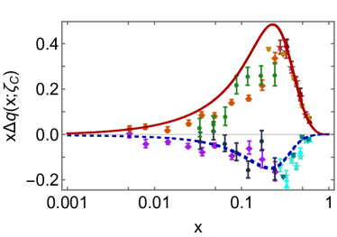
Figure 2: Polarised quark DFs: $\Delta{\mathpzc u}(x;\zeta_{\rm C})$ – solid red curves; and $\Delta{\mathpzc d}(x;\zeta_{\rm C})$ – dashed blue curves. Data: [48, HERMES] – circles; [49, COMPASS] – diamonds; filled down-triangles – [50, 51, 52, 53, CLAS EG1]; five-pointed stars – [54, E06-014]; filled up-triangles –[55, 56, E99-117].

  (a)

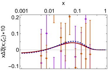
  (b)

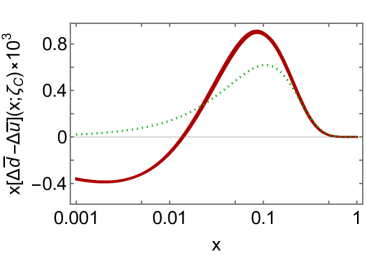
Figure 3: (a) Polarised antiquark DFs: $\Delta\bar{\mathpzc u}(x;\zeta_{\rm C})$ – solid red curves; and $\Delta\bar{\mathpzc d}(x;\zeta_{\rm C})$ – dashed blue curves. Data [49, COMPASS]: $\bar{\mathpzc u}$ – red diamonds; and $\bar{\mathpzc d}$ – purple squares. (b) $x[\Delta\bar{\mathpzc d}(x;\zeta_{\rm C})-\Delta\bar{\mathpzc u}(x;\zeta_{\rm C})]$ – solid red curves. For comparison: $x[\bar{\mathpzc d}(x;\zeta_{\rm C})-\bar{\mathpzc u}(x;\zeta_{\rm C})]$ – dotted green curve.

4 Polarised quark distributions at $\zeta^{2}=3\,$GeV²

With $\zeta_{\cal H}$ being that scale at which all properties of the proton are carried by its dressed valence quark dof, then the all-orders extension of QCD evolution explained in Refs. [68, 69, 70, 71] can be used to obtain all proton DFs at any scale $\zeta>\zeta_{\cal H}$. This approach has been used with success to predict proton and pion unpolarised DFs [65] and, recently, to extract the pion mass distribution from available data [72]. Herein, we use it to deliver predictions for proton polarised DFs.

This all-orders evolution scheme is based on a single proposition [69, 70, 71]:
    P1 – In the context of Refs. [73, 74], there exists at least one effective charge, $\alpha_{1\ell}(k^{2})$, which, when used to integrate the leading-order perturbative DGLAP equations, defines an evolution scheme for parton DFs that is all-orders exact.

Such charges need not be process-independent (PI); hence, not unique. Nevertheless, an efficacious PI charge is not excluded. That discussed in Refs. [68, 20, 69], denoted $\hat{\alpha}$, has proved suitable and we employ it herein. Using $\hat{\alpha}$, one predicts $\zeta_{\cal H}=0.331(2)\,$GeV. Connections with experiment and other nonperturbative extensions of QCD’s running coupling are given in Refs. [75, 76, 77].

Implemented as described in Ref. [65] and applied to the polarised valence DFs in Fig. 1, one obtains the $\zeta_{\rm C}=\surd 3\,$GeV polarised quark DFs drawn in Fig. 2, wherein they are compared with data inferred from experiments [48, HERMES], [49, COMPASS], [50, 51, 52, 53, CLAS EG1], [54, E06-014], [55, 56, E99-117]: there is agreement on the valence quark domain, $x\gtrsim 0.2$.

Referring to the COMPASS results, lying on $x\lesssim 0.2$, the collaboration’s extrapolations yield $g_{A}^{d}=-0.34(5)$, $g_{A}^{u}=0.71(4)$, $g_{A}=g_{A}^{u}-g_{A}^{d}=1.05(6)$. Comparison with Sec. 2-item (iv), shows agreement with our value of $g_{A}^{d}$. This is reflected in the match between data and our prediction for $\Delta{\mathpzc d}(x;\zeta_{\rm C})$. On the other hand, the data tend to lie below our prediction for $\Delta{\mathpzc u}(x;\zeta_{\rm C})$. This is understandable. The COMPASS results lead to a value for $g_{A}^{u}-g_{A}^{d}$ that is too small, viz. $0.83(5)$-times the value determined from neutron $\beta$-decay, an outcome which can be attributed to a low value of $g_{A}^{u}$: it is only $0.75(3)$-times our prediction. (These statements can be made because polarised antiquark DFs are negligible at this scale – see Figs. 3, 4.)

The polarised antiquark distributions are drawn in Fig. 3a along with values from Ref. [49, COMPASS]. On the scale of this image, set by the magnitudes of our predictions, the data have large uncertainties; so, can only be used to set plausible bounds on the size of these distributions.

The difference $x[\Delta\bar{\mathpzc d}(x;\zeta_{\rm C})-\Delta\bar{\mathpzc u}(x;\zeta_{\rm C})]$ is depicted in Fig. 3b and compared with the result for $x[\bar{\mathpzc d}(x;\zeta_{\rm C})-\bar{\mathpzc u}(x;\zeta_{\rm C})]$ from Refs. [29, 65], which reproduce the proton antimatter asymmetry reported in Ref. [78, SeaQuest]. (This was achieved via a modest Pauli blocking factor in the gluon splitting function.) Notably, both differences have the same magnitude; and their trend is similar on $x\gtrsim 0.01$: using P1, they are related. In this case, we do not report a comparison with data because the uncertainties on available results [48, HERMES], [49, COMPASS] are too large for such a comparison to be meaningful.

Our predictions for all polarised sea quark DFs are collected in Fig. 4. Following the implementation of all-orders evolution in Ref. [65], we have thresholds at which heavier quarks begin to play a role in evolution. This explains the flavour-separation amongst the polarised sea DFs. The image includes results on $2x\Delta{\mathpzc s}(x;\zeta_{\rm C})$ inferred from data in Ref.[49, COMPASS]. Broadly speaking, the magnitude matches our prediction for this DF; but, again, the data uncertainties are large. Our prediction $\int_{0.004}^{0.3}dx\,\Delta{\mathpzc s}_{S}(x;\zeta_{\rm C})=0.0072(1)$ is consistent with the inferred empirical value [49, COMPASS]: $-0.01\pm 0.01\pm 0.01$.

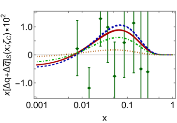
Figure 4: Polarised sea quark distributions at $\zeta_{\rm C}$. Solid red curves: $x[\Delta{\mathpzc u}+\Delta\bar{\mathpzc u}]_{S}$; dashed blue curves: $x[\Delta{\mathpzc d}+\Delta\bar{\mathpzc d}]_{S}$; $x[\Delta{\mathpzc s}+\Delta\bar{\mathpzc s}]_{S}$: dot-dashed green curves; $x[\Delta{\mathpzc c}+\Delta\bar{\mathpzc c}]_{S}$: dotted orange curves. Context is provided by values of $2x\Delta{\mathpzc s}(x;\zeta_{\rm C})$ from Ref.[49, COMPASS], wherein $x\Delta{\mathpzc s}(x;\zeta_{\rm C})\approx x\Delta\bar{\mathpzc s}(x;\zeta_{\rm C})$.

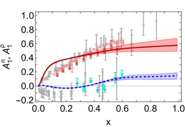
Figure 5: Predictions for proton (solid red) and neutron (dashed blue) longitudinal spin asymmetries at $\zeta_{\rm C}$. In each case, the associated band expresses the uncertainty deriving from Eq. (3). Data. $A_{1}^{p}$: red squares – Refs. [50, 51, 52, 53, CLAS EG1]; pink circles – Ref. [79]; grey up-triangles – Refs. [80, 81, 82, 83, 84, 85, 86, 87]. $A_{1}^{n}$: turquoise diamonds – Ref. [54, E06-014]; aqua five-pointed stars – Refs. [55, 56, E99-117]; grey down-triangles – Refs. [88, 89, 90, 91].

In Fig. 5, we depict our predictions for nucleon longitudinal spin asymmetries – defined, e.g., as in Ref. [92, Ch. 4.7]. (The $c$ quark contribution is practically negligible at this scale.) For context, we also show results inferred from data collected within the past vicennium [50, 51, 52, 53, 79, 54, 55, 56] and selected earlier results [80, 81, 82, 83, 84, 85, 86, 87, 88, 89, 90, 91]. The mismatch between prediction and inferences at low-$x$ may reflect known discrepancies between our predictions for sea quark DFs and those produced by phenomenological fits [20, 65]. On the other hand, there is general agreement between our predictions and data on $x\gtrsim 0.2$. New experiments able to return DF information on $x\gtrsim 0.6$ are desirable; especially in connection with the question of helicity retention discussed earlier. Thus, analyses of data collected recently [61, CLAS RGC], [62, E12-06-110] are much anticipated.

5 Polarised gluon distribution at $\zeta^{2}=3\,$GeV²

Beginning with the hadron-scale DFs in Fig. 1, the all-orders evolution scheme delivers the polarised and unpolarised gluon DFs at any scale $\zeta>\zeta_{\cal H}$. Our $\zeta_{\rm C}$ predictions are drawn in Fig. 6.

Insofar as phenomenological DF fits are concerned, $\Delta G(x)$ is very poorly constrained. This is illustrated by the grey band in Fig. 6a, drawn from Ref. [93, DSSV14] at $\zeta=10\,$GeV. At this scale, our central result is indicated by the dot-dashed (blue) curve. Evidently, as also seen with unpolarised DFs, on $x\lesssim 0.05$, our internally consistent predictions for glue (and sea) DFs are larger in magnitude than those inferred through phenomenological fits [20, 65]. Notwithstanding this, on the complementary domain we find

$$\int_{0.05}^{1}dx\,\Delta G(x;\zeta=10\,{\rm GeV})=0.199(3)\,,$$ (4)

cf.  $0.19(6)$ in Ref. [93, DSSV14].

  (a)

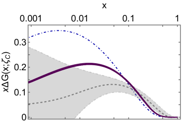
  (b)

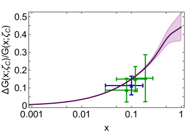
Figure 6: (a) Polarised gluon DF: $\Delta G(x;\zeta_{\rm C})$ – solid purple curves. Gray dashed curve and band: typical result from phenomenological global fit [93, DSSV14] reported at $\zeta=10\,$GeV. Evolved to this scale, our central prediction is the blue dot-dashed curve. (b) Polarised/unpolarised DF ratio $\Delta G(x;\zeta_{\rm C})/G(x;\zeta_{\rm C})$. The associated band expresses the uncertainty deriving from Eq. (3). For context, we depict values reported in Ref. [94, COMPASS].

Our prediction for the ratio $\Delta G(x;\zeta_{\rm C})/G(x;\zeta_{\rm C})$ is drawn in Fig. 6b. There is good agreement with the results reported in Ref. [94, COMPASS]. This is highlighted, e.g., by noting that the mean value of our result on the domain covered by measurements is $0.167(3)$ cf.  $0.113\pm 0.038\pm 0.036$ [94, COMPASS].

6 Proton spin

It is now appropriate to recall Eq. (2), which records that $\approx 65$% of the proton spin is carried by valence quark quasiparticle degrees of freedom at the hadron scale. Under P1, this value is independent of scale.

On the other hand, measurements of the proton spin are sensitive to the non-Abelian anomaly corrected combination [95]

$$a_{0}^{\rm E}(\zeta)=a_{0}-n_{f}\frac{\hat{\alpha}(\zeta)}{2\pi}\int_{0}^{1}dx\,\Delta G(x;\zeta)=:a_{0}-n_{f}\frac{\hat{\alpha}(\zeta)}{2\pi}\Delta G(\zeta)\,,$$ (5)

where $n_{f}$ is the number of active quark flavours: herein, $\hat{\alpha}$ and P1 evolution are defined using $n_{f}=4$.

Using our result for $\Delta G(x;\zeta_{\rm C})$ – Fig. 6 – to evaluate the right-hand side of Eq. (5), we predict

$$a_{0}^{\rm E}(\zeta_{\rm C})=0.35(2)\,.$$ (6)

This value compares favourably with that reported in Ref. [96, COMPASS]: $0.32(7)$.

Notwithstanding the remarks in the Introduction, it is common to report a light-front breakdown of the proton spin into contributions from quark and gluon spin and angular momenta:

$$\frac{1}{2}=\frac{1}{2}a_{0}+L_{q}(\zeta)+\Delta G(\zeta)+L_{g}(\zeta)\,.$$ (7)

This can be accomplished without ambiguity by exploiting the character of the hadron scale, viz.

$$L_{q}(\zeta_{\cal H})=\frac{1}{2}-\frac{1}{2}a_{0}=0.175\,,\Delta G(\zeta_{\cal H})=0=L_{g}(\zeta_{\cal H})\,,$$ (8)

and subsequently employing P1 evolution, which is implemented with minor modifications of Eqs. (32) in Ref. [57]. In this way, we determine the following central values:

$$L_{q}(\zeta_{\rm C})=-0.027\,,\;\Delta G(\zeta_{\rm C})=1.23\,,\;L_{g}(\zeta_{\rm C})=-1.03\,.$$ (9)

Evidently, although it begins positive, the light-front quark angular momentum fraction falls steadily with increasing scale; and the increasing gluon helicity is compensated by a growth in magnitude of the light-front gluon angular momentum fraction. The asymptotic ($\zeta\to\infty$) limits are discussed elsewhere [97, 98].

7 Summary and Outlook

Beginning with Ansätze for proton hadron-scale polarised valence quark distribution functions, developed using insights from perturbative QCD and constrained by solutions of a quark+diquark Faddeev equation, and supposing that there is an effective charge which defines an evolution scheme for parton DFs – both unpolarised and polarised – that is all-orders exact, we delivered parameter-free predictions for all proton polarised DFs at the scale $\zeta_{\rm C}^{2}=3\,$GeV². In doing so, we completed a unification of proton and pion DFs. All predictions, both pointwise behaviour and moments, compare favourably with results inferred from data, as exemplified herein by our results for polarised quark DFs [Fig. 2] and nucleon longitudinal spin asymmetries [Fig. 5].

Of particular significance is our finding that the polarised gluon DF, $\Delta G(x;\zeta_{\rm C})$, in the proton is positive and large [Fig. 6]. This prediction can be tested using experiments at next-generation QCD facilities [99, 100]. Meanwhile, our result for $\Delta G(x;\zeta_{\rm C})$ enables us to predict that measurements of the proton singlet axial charge should return a value $a_{0}^{\rm E}(\zeta_{\rm C})=0.35(2)$. This result is in accord with contemporary data.

Our analysis can be tested and improved in future by using a recently developed symmetry preserving axial current, appropriate for a proton described as a bound state of dressed-quark and fully interacting nonpointlike diquark degrees-of-freedom, to calculate the proton hadron scale polarised valence quark DFs. A first step in this direction is underway using a careful treatment of a momentum-independent quark+quark interaction. Its extension to a study of the proton using QCD-connected Schwinger functions is thereafter natural. Longer term goals include analogous calculations that begin with a Poincaré-covariant three-body treatment of the nucleon bound state problem [2, 3].

Acknowledgments. We are grateful for assistance and constructive comments from A. Deur, T. Liu and C. Mondal. Work supported by: National Natural Science Foundation of China (grant nos. 12135007, 12247103); Natural Science Foundation of Jiangsu Province (grant no. BK20220323).

Declaration of Competing Interest. The authors declare that they have no known competing financial interests or personal relationships that could have appeared to influence the work reported in this paper.

References

- Brodsky et al. [2022] S. J. Brodsky, A. Deur, C. D. Roberts, Artificial dynamical effects in quantum field theory, Nature Rev. Phys. 4 (7) (2022) 489–495.
- Eichmann et al. [2010] G. Eichmann, R. Alkofer, A. Krassnigg, D. Nicmorus, Nucleon mass from a covariant three-quark Faddeev equation, Phys. Rev. Lett. 104 (2010) 201601.
- Wang et al. [2018] Q.-W. Wang, S.-X. Qin, C. D. Roberts, S. M. Schmidt, Proton tensor charges from a Poincaré-covariant Faddeev equation, Phys. Rev. D 98 (2018) 054019.
- Ashman et al. [1988] J. Ashman, et al., A Measurement of the Spin Asymmetry and Determination of the Structure Function in Deep Inelastic Muon-Proton Scattering, Phys. Lett. B 206 (1988) 364.
- Brodsky and Lepage [1989] S. J. Brodsky, G. P. Lepage, Exclusive Processes in Quantum Chromodynamics, Adv. Ser. Direct. High Energy Phys. 5 (1989) 93–240.
- Brodsky et al. [1998] S. J. Brodsky, H.-C. Pauli, S. S. Pinsky, Quantum chromodynamics and other field theories on the light cone, Phys. Rept. 301 (1998) 299–486.
- Heinzl [2001] T. Heinzl, Light cone quantization: Foundations and applications, Lect. Notes Phys. 572 (2001) 55–142.
- Eichmann et al. [2016] G. Eichmann, H. Sanchis-Alepuz, R. Williams, R. Alkofer, C. S. Fischer, Baryons as relativistic three-quark bound states, Prog. Part. Nucl. Phys. 91 (2016) 1–100.
- Qin and Roberts [2020] S.-X. Qin, C. D. Roberts, Impressions of the Continuum Bound State Problem in QCD, Chin. Phys. Lett. 37 (12) (2020) 121201.
- Roberts et al. [2021] C. D. Roberts, D. G. Richards, T. Horn, L. Chang, Insights into the emergence of mass from studies of pion and kaon structure, Prog. Part. Nucl. Phys. 120 (2021) 103883.
- Binosi [2022] D. Binosi, Emergent Hadron Mass in Strong Dynamics, Few Body Syst. 63 (2) (2022) 42.
- Roberts [2023] C. D. Roberts, Origin of the Proton Mass, EPJ Web Conf. 282 (2023) 01006.
- Papavassiliou [2022] J. Papavassiliou, Emergence of mass in the gauge sector of QCD, Chin. Phys. C 46 (11) (2022) 112001.
- Ding et al. [2023] M. Ding, C. D. Roberts, S. M. Schmidt, Emergence of Hadron Mass and Structure, Particles 6 (1) (2023) 57–120.
- Salmè [2022] G. Salmè, Explaining mass and spin in the visible matter: the next challenge, J. Phys. Conf. Ser. 2340 (1) (2022) 012011.
- Ferreira and Papavassiliou [2023] M. N. Ferreira, J. Papavassiliou, Gauge Sector Dynamics in QCD, Particles 6 (1) (2023) 312–363.
- Carman et al. [2023] D. S. Carman, R. W. Gothe, V. I. Mokeev, C. D. Roberts, Nucleon Resonance Electroexcitation Amplitudes and Emergent Hadron Mass, Particles 6 (1) (2023) 416–439.
- Ding et al. [2020] M. Ding, K. Raya, D. Binosi, L. Chang, C. D. Roberts, S. M. Schmidt, Drawing insights from pion parton distributions, Chin. Phys. C (Lett.) 44 (2020) 031002.
- Cui et al. [2021] Z.-F. Cui, M. Ding, F. Gao, K. Raya, D. Binosi, L. Chang, C. D. Roberts, J. Rodríguez-Quintero, S. M. Schmidt, Higgs modulation of emergent mass as revealed in kaon and pion parton distributions, Eur. Phys. J. A (Lett.) 57 (1) (2021) 5.
- Cui et al. [2020a] Z.-F. Cui, M. Ding, F. Gao, K. Raya, D. Binosi, L. Chang, C. D. Roberts, J. Rodríguez-Quintero, S. M. Schmidt, Kaon and pion parton distributions, Eur. Phys. J. C 80 (2020a) 1064.
- Roberts [2017] C. D. Roberts, Perspective on the origin of hadron masses, Few Body Syst. 58 (2017) 5.
- Cahill et al. [1987] R. T. Cahill, C. D. Roberts, J. Praschifka, Calculation of diquark masses in QCD, Phys. Rev. D 36 (1987) 2804.
- Barabanov et al. [2021] M. Y. Barabanov, et al., Diquark Correlations in Hadron Physics: Origin, Impact and Evidence, Prog. Part. Nucl. Phys. 116 (2021) 103835.
- Cahill et al. [1989] R. T. Cahill, C. D. Roberts, J. Praschifka, Baryon structure and QCD, Austral. J. Phys. 42 (1989) 129–145.
- Reinhardt [1990] H. Reinhardt, Hadronization of Quark Flavor Dynamics, Phys. Lett. B 244 (1990) 316–326.
- Efimov et al. [1990] G. V. Efimov, M. A. Ivanov, V. E. Lyubovitskij, Quark - diquark approximation of the three quark structure of baryons in the quark confinement model, Z. Phys. C 47 (1990) 583–594.
- Mezrag et al. [2018] C. Mezrag, J. Segovia, L. Chang, C. D. Roberts, Parton distribution amplitudes: Revealing correlations within the proton and Roper, Phys. Lett. B 783 (2018) 263–267.
- Liu et al. [2022] L. Liu, C. Chen, Y. Lu, C. D. Roberts, J. Segovia, Composition of low-lying -baryons, Phys. Rev. D 105 (11) (2022) 114047.
- Chang et al. [2022] L. Chang, F. Gao, C. D. Roberts, Parton distributions of light quarks and antiquarks in the proton, Phys. Lett. B 829 (2022) 137078.
- Workman et al. [2022] R. L. Workman, et al., Review of Particle Physics, PTEP 2022 (2022) 083C01.
- Chen and Roberts [2022] C. Chen, C. D. Roberts, Nucleon axial form factor at large momentum transfers, Eur. Phys. J. A 58 (2022) 206.
- Cheng et al. [2022] P. Cheng, F. E. Serna, Z.-Q. Yao, C. Chen, Z.-F. Cui, C. D. Roberts, Contact interaction analysis of octet baryon axial-vector and pseudoscalar form factors, Phys. Rev. D 106 (5) (2022) 054031.
- Chen et al. [2021] C. Chen, C. S. Fischer, C. D. Roberts, J. Segovia, Form Factors of the Nucleon Axial Current, Phys. Lett. B 815 (2021) 136150.
- Chen et al. [2022] C. Chen, C. S. Fischer, C. D. Roberts, J. Segovia, Nucleon axial-vector and pseudoscalar form factors and PCAC relations, Phys. Rev. D 105 (9) (2022) 094022.
- Liu et al. [2020] T. Liu, R. S. Sufian, G. F. de Téramond, H. G. Dosch, S. J. Brodsky, A. Deur, Unified Description of Polarized and Unpolarized Quark Distributions in the Proton, Phys. Rev. Lett. 124 (8) (2020) 082003.
- Han et al. [2022] C. Han, G. Xie, R. Wang, X. Chen, An analysis of polarized parton distribution functions with nonlinear QCD evolution equations, Nucl. Phys. B 985 (2022) 116012.
- Brodsky et al. [1995] S. J. Brodsky, M. Burkardt, I. Schmidt, Perturbative QCD constraints on the shape of polarized quark and gluon distributions, Nucl. Phys. B 441 (1995) 197–214.
- Brisudova et al. [2000] M. M. Brisudova, L. Burakovsky, J. T. Goldman, Effective functional form of Regge trajectories, Phys. Rev. D 61 (2000) 054013.
- Roberts et al. [2013] C. D. Roberts, R. J. Holt, S. M. Schmidt, Nucleon spin structure at very high , Phys. Lett. B 727 (2013) 249–254.
- Close and Thomas [1988] F. E. Close, A. W. Thomas, The Spin and Flavor Dependence of Parton Distribution Functions, Phys. Lett. B 212 (1988) 227.
- Hughes and Voss [1999] E. W. Hughes, R. Voss, Spin structure functions, Ann. Rev. Nucl. Part. Sci. 49 (1999) 303–339.
- Farrar and Jackson [1975] G. R. Farrar, D. R. Jackson, Pion and Nucleon Structure Functions Near , Phys. Rev. Lett. 35 (1975) 1416.
- Holt and Roberts [2010] R. J. Holt, C. D. Roberts, Distribution Functions of the Nucleon and Pion in the Valence Region, Rev. Mod. Phys. 82 (2010) 2991–3044.
- Dokshitzer [1977] Y. L. Dokshitzer, Calculation of the Structure Functions for Deep Inelastic Scattering and Annihilation by Perturbation Theory in Quantum Chromodynamics. (In Russian), Sov. Phys. JETP 46 (1977) 641–653.
- Gribov and Lipatov [1971] V. N. Gribov, L. N. Lipatov, Deep inelastic electron scattering in perturbation theory, Phys. Lett. B 37 (1971) 78–80.
- Lipatov [1975] L. N. Lipatov, The parton model and perturbation theory, Sov. J. Nucl. Phys. 20 (1975) 94–102.
- Altarelli and Parisi [1977] G. Altarelli, G. Parisi, Asymptotic Freedom in Parton Language, Nucl. Phys. B 126 (1977) 298–318.
- Airapetian et al. [2005] A. Airapetian, et al., Quark helicity distributions in the nucleon for up, down, and strange quarks from semi-inclusive deep-inelastic scattering, Phys. Rev. D 71 (2005) 012003.
- Alekseev et al. [2010] M. G. Alekseev, et al., Quark helicity distributions from longitudinal spin asymmetries in muon-proton and muon-deuteron scattering, Phys. Lett. B 693 (2010) 227–235.
- Dharmawardane et al. [2006] K. V. Dharmawardane, et al., Measurement of the - and -dependence of the asymmetry on the nucleon, Phys. Lett. B 641 (2006) 11–17.
- Prok et al. [2009] Y. Prok, et al., Moments of the Spin Structure Functions and for -GeV2, Phys. Lett. B 672 (2009) 12–16.
- Guler et al. [2015] N. Guler, et al., Precise determination of the deuteron spin structure at low to moderate with CLAS and extraction of the neutron contribution, Phys. Rev. C 92 (5) (2015) 055201.
- Fersch et al. [2017] R. Fersch, et al., Determination of the Proton Spin Structure Functions for using CLAS, Phys. Rev. C 96 (6) (2017) 065208.
- Parno et al. [2015] D. S. Parno, et al., Precision Measurements of in the Deep Inelastic Regime, Phys. Lett. B 744 (2015) 309–314.
- Zheng et al. [2004a] X. Zheng, et al., Precision measurement of the neutron spin asymmetry and spin flavor decomposition in the valence quark region, Phys. Rev. Lett. 92 (2004a) 012004.
- Zheng et al. [2004b] X. Zheng, et al., Precision measurement of the neutron spin asymmetries and spin-dependent structure functions in the valence quark region, Phys. Rev. C 70 (2004b) 065207.
- Deur et al. [2019] A. Deur, S. J. Brodsky, G. F. De Téramond, The Spin Structure of the Nucleon, Rept. Prog. Phys. 82 (076201).
- Xu et al. [2021] S. Xu, C. Mondal, J. Lan, X. Zhao, Y. Li, J. P. Vary, Nucleon structure from basis light-front quantization, Phys. Rev. D 104 (9) (2021) 094036.
- Xu et al. [2022] S. Xu, C. Mondal, X. Zhao, Y. Li, J. P. Vary, Nucleon spin decomposition with one dynamical gluon – arXiv:2209.08584 [hep-ph] .
- Ethier and Nocera [2020] J. J. Ethier, E. R. Nocera, Parton Distributions in Nucleons and Nuclei, Ann. Rev. Nucl. Part. Sci. 70 (2020) 43–76.
- Kuhn et al. [ 109] S. Kuhn, et al., The Longitudinal Spin Structure of the Nucleon, CLAS Collaboration (E12-06-109).
- Zheng et al. [tion] X. Zheng, et al., Measurement of Neutron Spin Asymmetry A in the Valence Quark Region using an 11 GeV Beam and a Polarized 3He Target in Hall C, E12-06-110 Collaboration.
- Bali et al. [2016] G. S. Bali, et al., Light-cone distribution amplitudes of the baryon octet, JHEP 02 (2016) 070.
- Lepage and Brodsky [1980] G. P. Lepage, S. J. Brodsky, Exclusive Processes in Perturbative Quantum Chromodynamics, Phys. Rev. D 22 (1980) 2157–2198.
- Lu et al. [2022] Y. Lu, L. Chang, K. Raya, C. D. Roberts, J. Rodríguez-Quintero, Proton and pion distribution functions in counterpoint, Phys. Lett. B 830 (2022) 137130.
- Abrams et al. [2022] D. Abrams, et al., Measurement of the Nucleon Structure Function Ratio by the Jefferson Lab MARATHON Tritium/Helium-3 Deep Inelastic Scattering Experiment, Phys. Rev. Lett. 128 (13) (2022) 132003.
- Cui et al. [2022a] Z.-F. Cui, F. Gao, D. Binosi, L. Chang, C. D. Roberts, S. M. Schmidt, Valence quark ratio in the proton, Chin. Phys. Lett. Express 39 (04) (2022a) 041401.
- Cui et al. [2020b] Z.-F. Cui, J.-L. Zhang, D. Binosi, F. de Soto, C. Mezrag, J. Papavassiliou, C. D. Roberts, J. Rodríguez-Quintero, J. Segovia, S. Zafeiropoulos, Effective charge from lattice QCD, Chin. Phys. C 44 (2020b) 083102.
- Raya et al. [2022] K. Raya, Z.-F. Cui, L. Chang, J.-M. Morgado, C. D. Roberts, J. Rodríguez-Quintero, Revealing pion and kaon structure via generalised parton distributions, Chin. Phys. C 46 (26) (2022) 013105.
- Cui et al. [2022b] Z. F. Cui, M. Ding, J. M. Morgado, K. Raya, D. Binosi, L. Chang, J. Papavassiliou, C. D. Roberts, J. Rodríguez-Quintero, S. M. Schmidt, Concerning pion parton distributions, Eur. Phys. J. A 58 (1) (2022b) 10.
- Cui et al. [2022c] Z. F. Cui, M. Ding, J. M. Morgado, K. Raya, D. Binosi, L. Chang, F. De Soto, C. D. Roberts, J. Rodríguez-Quintero, S. M. Schmidt, Emergence of pion parton distributions, Phys. Rev. D 105 (9) (2022c) L091502.
- Xu et al. [2023] Y.-Z. Xu, K. Raya, Z.-F. Cui, C. D. Roberts, J. Rodríguez-Quintero, Empirical Determination of the Pion Mass Distribution, Chin. Phys. Lett. Express 40 (4) (2023) 041201.
- Grunberg [1980] G. Grunberg, Renormalization Group Improved Perturbative QCD, Phys. Lett. B 95 (1980) 70, [Erratum: Phys. Lett. B 110, 501 (1982)].
- Grunberg [1984] G. Grunberg, Renormalization Scheme Independent QCD and QED: The Method of Effective Charges, Phys. Rev. D 29 (1984) 2315.
- Deur et al. [2016] A. Deur, S. J. Brodsky, G. F. de Teramond, The QCD Running Coupling, Prog. Part. Nucl. Phys. 90 (2016) 1–74.
- Deur et al. [2022] A. Deur, V. Burkert, J. P. Chen, W. Korsch, Experimental determination of the QCD effective charge , Particles 5 (2) (2022) 171–179.
- Deur et al. [2023] A. Deur, S. J. Brodsky, C. D. Roberts, QCD Running Couplings and Effective Charges – arXiv:2303.00723 [hep-ph] .
- Dove et al. [2021] J. Dove, et al., The asymmetry of antimatter in the proton, Nature 590 (7847) (2021) 561–565.
- Prok et al. [2014] Y. Prok, et al., Precision measurements of of the proton and the deuteron with 6 GeV electrons, Phys. Rev. C 90 (2) (2014) 025212.
- Anthony et al. [1999] P. L. Anthony, et al., Measurement of the deuteron spin structure function for 1-(GeV/c)-(GeV/c)2, Phys. Lett. B 463 (1999) 339–345.
- Anthony et al. [2000] P. L. Anthony, et al., Measurements of the dependence of the proton and neutron spin structure functions and , Phys. Lett. B 493 (2000) 19–28.
- Airapetian et al. [1998] A. Airapetian, et al., Measurement of the proton spin structure function g1(p) with a pure hydrogen target, Phys. Lett. B 442 (1998) 484–492.
- Abe et al. [1995] K. Abe, et al., Measurements of the dependence of the proton and deuteron spin structure functions and , Phys. Lett. B 364 (1995) 61–68.
- Abe et al. [1997a] K. Abe, et al., Measurements of the proton and deuteron spin structure function in the resonance region, Phys. Rev. Lett. 78 (1997a) 815–819.
- Abe et al. [1998] K. Abe, et al., Measurements of the proton and deuteron spin structure functions and , Phys. Rev. D 58 (1998) 112003.
- Adams et al. [1994] D. Adams, et al., Measurement of the spin dependent structure function of the proton, Phys. Lett. B 329 (1994) 399–406, [Erratum: Phys. Lett. B 339, 332–333 (1994)].
- Adams et al. [1997] D. Adams, et al., Spin structure of the proton from polarized inclusive deep inelastic muon - proton scattering, Phys. Rev. D 56 (1997) 5330–5358.
- Ackerstaff et al. [1997] K. Ackerstaff, et al., Measurement of the neutron spin structure function with a polarized He internal target, Phys. Lett. B 404 (1997) 383–389.
- Abe et al. [1997b] K. Abe, et al., Precision determination of the neutron spin structure function , Phys. Rev. Lett. 79 (1997b) 26–30.
- Abe et al. [1997c] K. Abe, et al., Next-to-leading order QCD analysis of polarized deep inelastic scattering data, Phys. Lett. B 405 (1997c) 180–190.
- Anthony et al. [1996] P. L. Anthony, et al., Deep inelastic scattering of polarized electrons by polarized He and the study of the neutron spin structure, Phys. Rev. D 54 (1996) 6620–6650.
- Ellis et al. [1991] R. K. Ellis, W. J. Stirling, B. R. Webber, QCD and collider physics, Cambridge University Press, Cambridge, UK, 1991.
- de Florian et al. [2014] D. de Florian, R. Sassot, M. Stratmann, W. Vogelsang, Evidence for polarization of gluons in the proton, Phys. Rev. Lett. 113 (1) (2014) 012001.
- Adolph et al. [2017a] C. Adolph, et al., Leading-order determination of the gluon polarisation from semi-inclusive deep inelastic scattering data, Eur. Phys. J. C 77 (4) (2017a) 209.
- Altarelli and Ross [1988] G. Altarelli, G. G. Ross, The Anomalous Gluon Contribution to Polarized Leptoproduction, Phys. Lett. B 212 (1988) 391–396.
- Adolph et al. [2017b] C. Adolph, et al., Final COMPASS results on the deuteron spin-dependent structure function and the Bjorken sum rule, Phys. Lett. B 769 (2017b) 34–41.
- Ji et al. [1996] X.-D. Ji, J. Tang, P. Hoodbhoy, The spin structure of the nucleon in the asymptotic limit, Phys. Rev. Lett. 76 (1996) 740–743.
- Chen et al. [2011] X.-S. Chen, W.-M. Sun, F. Wang, T. Goldman, Proper identification of the gluon spin, Phys. Lett. B 700 (2011) 21–24.
- Anderle et al. [2021] D. P. Anderle, et al., Electron-ion collider in China, Front. Phys. (Beijing) 16 (6) (2021) 64701.
- Abdul Khalek et al. [2022] R. Abdul Khalek, et al., Science Requirements and Detector Concepts for the Electron-Ion Collider: EIC Yellow Report, Nucl. Phys. A 1026 (2022) 122447.