Robust, randomized preconditioning for kernel ridge regression

Abstract

This paper introduces two randomized preconditioning techniques for robustly solving kernel ridge regression (KRR) problems with a medium to large number of data points ($10^{4}\leq N\leq 10^{7}$). The first method, RPCholesky preconditioning, is capable of accurately solving the full-data KRR problem in $\mathcal{O}(N^{2})$ arithmetic operations, assuming sufficiently rapid polynomial decay of the kernel matrix eigenvalues. The second method, KRILL preconditioning, offers an accurate solution to a restricted version of the KRR problem involving $k\ll N$ selected data centers at a cost of $\mathcal{O}((N+k^{2})k\log k)$ operations. The proposed methods efficiently solve a broad range of KRR problems and overcome the failure modes of previous KRR preconditioners, making them ideal for practical applications.

1 Motivation

Kernel ridge regression (KRR) is a machine learning method for learning an unknown function $y=f(\bm{x})$ from a set of input–output pairs

$$(\bm{x}^{(1)},y_{1}),(\bm{x}^{(2)},y_{2}),\ldots,(\bm{x}^{(N)},y_{N})\in\mathcal{X}\times\mathbb{R},$$

where the inputs take values in an arbitrary set $\mathcal{X}$. KRR is based on a positive-definite kernel $K$, a function on $\mathcal{X}\times\mathcal{X}$ that captures the “similarity” between a pair of inputs. KRR produces a nonlinear prediction function $\widehat{f}:\mathcal{X}\to\mathbb{R}$ of the form

$$\widehat{f}(\bm{x})=\sum\nolimits_{i=1}^{N}\beta_{i}K(\bm{x}^{(i)},\bm{x})$$

that models the input–output relationship. KRR is widely used in data science and scientific computing, for example, in predicting the chemical properties of molecules [15, 41]. More details about KRR are provided in Section 2.

In practice, KRR is often limited to small- or medium-sized data sets ($N\leq 10^{4}$) because the computation time can grow rapidly with the number of data points. KRR involves linear algebra computations with the $N\times N$ kernel matrix $\bm{A}$ with entries $a_{ij}=K(\bm{x}^{(i)},\bm{x}^{(j)})$. To obtain the prediction function $\widehat{f}$, we must solve an $N\times N$ positive-definite linear system to high accuracy, which requires $\mathcal{O}(N^{3})$ arithmetic operations using the standard direct method based on Cholesky decomposition. Because of this poor computational scaling, survey articles on machine learning for scientific audiences (such as [38]) suggest using KRR for small data sets and neural networks for larger data sets. Reliably scaling KRR to larger data sets with $N\geq 10^{4}$ remains an open research challenge.

To improve the scalability of KRR, two main approaches have been developed. The first approach aims to solve the full-data KRR problem accurately in $\mathcal{O}(N^{2})$ operations using preconditioned conjugate gradient (CG) [13, 4]. The second approach restricts the KRR problem to a small number of $k\ll N$ centers chosen from the data points [35] and aims to solve the restricted problem in $\mathcal{O}(kN)$ operations using preconditioned CG [32].

However, due to the ill-conditioned nature of many KRR problems, CG-based approaches can only succeed when there is a high-quality preconditioner. Consequently, much of the research on solving KRR problems over the past decade has focused on proposing preconditioners [13, 32, 19, 33, 18], empirically testing preconditioners [13, 7], and theoretically analyzing preconditioners [4, 32, 19, 33, 18]. Despite this extensive body of work, the available preconditioners are either expensive to construct or prone to failure when applied to specific KRR problems, hindering their usefulness in real-world scenarios.

The primary purpose of a preconditioner is to minimize the number of CG iterations required to solve a linear system to a desired level of accuracy. For KRR, each CG iteration can be computationally expensive as it involves either one multiplication with the $N\times N$ kernel matrix (for full-data KRR) or two multiplications with the $N\times k$ kernel submatrix (for restricted KRR). Additionally, the kernel matrix or submatrix may not fit in working memory, in which case kernel matrix entries must be accessed from storage or regenerated from data at each CG iteration, which adds to the computational cost. This paper seeks to reduce the expense of KRR by proposing new preconditioners that are both efficient to construct and capable of controlling the number of CG iterations required for convergence.

To be useful in practice, a preconditioner must work reliably for a range of KRR instances, and it must be robust against adverse conditions (such as poorly conditioned kernel matrices). Additionally, the preconditioner should not require any delicate parameter tuning. Such a robust and no-hassle preconditioner is vital for general-purpose scientific software that can handle a variety of KRR problems framed by different users. Additionally, such a preconditioner is critical for cross-validation, as it enables searching for the best kernel model while having confidence that the preconditioner can handle the resulting linear systems efficiently.

In this paper, we propose randomized preconditioners that allow us to solve more KRR problems in fewer iterations than the techniques in current use [13, 32, 19, 33, 18]. Our preconditioners are based on randomized constructions [10, 12] that have not been previously applied in the context of KRR but are important for achieving robustness. We devise two new methods: the RPCholesky preconditioner (Algorithm 1) accurately solves the full-data KRR problem, and the KRILL preconditioner (Algorithm 2) accurately solves the restricted KRR problem involving $k\ll N$ data centers. Both preconditioners are cheap to implement, are effective for a wide range of KRR problems, and are supported by strong theoretical guarantees.

1.1 Plan for paper

The rest of this paper is organized as follows. Section 2 presents the RPCholesky and KRILL preconditioning strategies; Section 3 compares RPCholesky and KRILL to other preconditioners; Section 4 applies the RPCholesky and KRILL preconditioners to benchmark problems in computational chemistry and physics; Section 5 contains proofs of the theoretical results; and Section 6 offers conclusions.

1.2 Notation

For simplicity, we focus on the real setting, although our work extends to complex-valued kernels without significant modification. The transpose and Moore–Penrose pseudoinverse of $\bm{A}$ are denoted $\bm{A}^{*}$ and $\bm{A}^{\dagger}$. Double bars $\left\|\cdot\right\|$ indicate the Euclidean norm of a vector or the spectral norm of a matrix. The matrix condition number is $\kappa(\bm{A})\coloneqq\lVert\bm{A}\rVert\lVert\bm{A}^{-1}\rVert$. For a positive-definite matrix $\bm{M}$, the $\bm{M}$-weighted inner product norm is denoted $\lVert\bm{z}\rVert_{\bm{M}}\coloneqq(\bm{z}^{*}\bm{M}\bm{z})^{1/2}$. The function $\lambda_{i}(\bm{M})$ outputs the $i$th largest eigenvalue of $\bm{M}.$ The $\ell_{1}$ norm of the vector $\bm{x}$ is denoted by $\|\bm{x}\|_{\ell_{1}}=\sum_{i}|x_{i}|$. The symbol $|\mathsf{S}|$ denotes the cardinality of a set $\mathsf{S}$.

2 Algorithms and initial evidence

This section introduces the full-data KRR problem (Section 2.1) and the restricted KRR problem (Section 2.2), and it describes our RPCholesky and KRILL preconditioners for solving these problems.

2.1 Full-data kernel ridge regression

Recall that we are given $N$ input–output data pairs $(\bm{x}^{(1)},y_{1}),(\bm{x}^{(2)},y_{2}),\ldots,(\bm{x}^{(N)},y_{N})$ in $\mathcal{X}\times\mathbb{R}$ for training. Assume that $K(\cdot,\cdot)$ is a positive-definite kernel function on $\mathcal{X}\times\mathcal{X}$, and define the $N\times N$ positive-semidefinite kernel matrix $\bm{A}$ with numerical entries $a_{ij}=K(\bm{x}^{(i)},\bm{x}^{(j)})$.

In the full-data kernel ridge regression (KRR), we build a prediction function of the form

$$\widehat{f}(\bm{x};\bm{\beta})=\sum\nolimits_{i=1}^{N}\beta_{i}K(\bm{x}^{(i)},\bm{x}).$$

The coefficients $\bm{\beta}\in\mathbb{R}^{N}$ for the function are chosen to minimize the regularized least-squares loss function

$$L(\bm{\beta})=\lVert\bm{y}-\bm{A}\bm{\beta}\rVert^{2}+\mu\bm{\beta}^{\ast}\bm{A}\bm{\beta}.$$

Here, $\mu>0$ is a regularization parameter, typically chosen through cross-validation using a separate set of validation data.

Minimizing $L(\bm{\beta})$ is a quadratic optimization problem whose solution $\bm{\beta}$ satisfies

$$(\bm{A}+\mu\mathbf{I})\bm{\beta}=\bm{y}.$$ (2.1)

We can solve this linear system in $\mathcal{O}(N^{3})$ time using a Cholesky decomposition of $\bm{A}+\mu\mathbf{I}$ and two triangular solves. However, if there is a medium or large number of data points ($N\geq 10^{4}$), we recommend solving (2.1) at a reduced cost using conjugate gradient with RPCholesky preconditioning, described below. We will prove that RPCholesky solves the full-data KRR problem in $\mathcal{O}(N^{2})$ time, provided the kernel matrix eigenvalues decay sufficiently quickly (Theorem 2.2).

2.1.1 RPCholesky preconditioning

Algorithm 1 RPCholesky preconditioning

1:Positive semidefinite matrix $\bm{A}\in{}^{N\times N}$, right-hand-side vector $\bm{y}\in{}^{N}$, regularization coefficient $\mu$, approximation rank $r$, and tolerance $\varepsilon$.

2:Approximate solution $\bm{\beta}_{\star}$ to $(\bm{A}+\mu\,\mathbf{I})\bm{\beta}=\bm{y}$.

3:$\bm{F}\leftarrow\textsc{RPCholesky}(\bm{A},r,\min(100,r/10))$ $\triangleright$ See Algorithm 4

4:$(\bm{U},\bm{\Sigma},\sim)\leftarrow\textsc{EconomySizeSVD}(\bm{F})$ $\triangleright$ $\bm{\widehat{A}}=\bm{U}\bm{\Sigma}^{2}\bm{U}^{*}$

5:Define primitives for preconditioned conjugate gradient:

Product $$:\bm{\beta}\mapsto\bm{A}\bm{\beta}+\mu\bm{\beta}$$

Preconditioner $$:\bm{\beta}\mapsto\bm{U}\left[(\bm{\Sigma}^{2}+\mu\mathbf{I})^{-1}-\mu^{-1}\mathbf{I}\right]\bm{U}^{*}\bm{\beta}+\mu^{-1}\bm{\beta}$$

6:$\bm{\beta}_{\star}\leftarrow\textsc{PCG}(\texttt{Product},\bm{y},\varepsilon,\texttt{Preconditioner})$ $\triangleright$ See Algorithm 3

To build a preconditioner for the full-data KRR equations (2.1), we begin with a low-rank approximation $\bm{\widehat{A}}$ of the kernel matrix $\bm{A}$. Then, we construct the preconditioner

$$\bm{P}=\bm{\widehat{A}}+\mu\mathbf{I}.$$ (2.2)

There are many ways to obtain a low-rank approximation for this purpose, and we adopt the newly developed RPCholesky algorithm (Algorithm 4, proposed in [10]).

The RPCholesky algorithm is a variant of partial Cholesky decomposition that chooses random pivots at each step according to an evolving probability distribution. For an input parameter $r\in\mathbb{N}$, the algorithm returns a rank-$r$ approximation in factorized form:

$$\bm{\widehat{A}}=\bm{F}\bm{F}^{\ast}\quad\text{where}\quad\bm{F}\in{}^{N\times r}.$$

The matrix $\bm{\widehat{A}}$ is random because it depends on the choice of random pivots. On average, $\bm{\widehat{A}}$ compares well with the best rank-$r$ approximation of $\bm{A}$, as established in [10, Thm. 3.1]. The algorithm accesses only $(r+1)N$ entries of the kernel matrix; it uses $\mathcal{O}(rN)$ storage; and it expends $\mathcal{O}(r^{2}N)$ arithmetic operations.

We propose to select the approximation rank $r=\mathcal{O}(\sqrt{N})$, which ensures that we can obtain an eigenvalue decomposition of the preconditioner $\bm{P}$ in $\mathcal{O}(N^{2})$ operations. We then apply preconditioned CG (Algorithm 3, described in [20, §10.3]) to solve the KRR problem. Provided that $r=\mathcal{O}(\sqrt{N})$ suffices to obtain a good preconditioner, CG terminates in a constant number of iterations, and the total operation count for RPCholesky preconditioning is $\mathcal{O}(N^{2})$. We provide pseudocode for this RPCholesky preconditioning approach in Algorithm 1.

2.1.2 Empirical performance

Figure 1 shows RPCholesky’s performance across 21 regression and classification KRR problems, summarized in Table 1 of Appendix A. To make the figure, we first randomly subsample $N=1.5\times 10^{4}$ data points for each problem. We standardize the features (subtract the mean, divide by the standard deviation) and measure similarity with the squared exponential kernel

$$K(\bm{x},\bm{y})=\exp\bigl{(}-\tfrac{1}{2\sigma^{2}}\lVert\bm{x}-\bm{y}\rVert^{2}\bigr{)}\quad\text{with bandwidth $\sigma=3$.}$$ (2.3)

We then formulate the KRR problem (2.1) with a regularization parameter $\mu/N=10^{-7}$ and choose the rank $r$ of the preconditioner to be either $r=500$ (left panel) or $r=1000$ (right panel). Our choice of parameters is typical for full-data KRR problems [4, 18], and we apply the same parameters uniformly over the 21 regression and classification problems without any additional tuning. The small value of $\mu$ makes many of these problems highly ill-conditioned.

We run 250 CG iterations and declare each KRR instance to be “solved” as soon as the relative residual $\lVert(\bm{A}+\mu\mathbf{I})\bm{x}-\bm{y}\rVert/\lVert\bm{y}\rVert$ falls below an error tolerance of $\varepsilon=10^{-3}$. This choice of $\varepsilon$ is justified by the fact that the test error plateaus after reaching this tolerance for all of the problems we considered.

$\qquad r=500$

$\qquad r=1000$

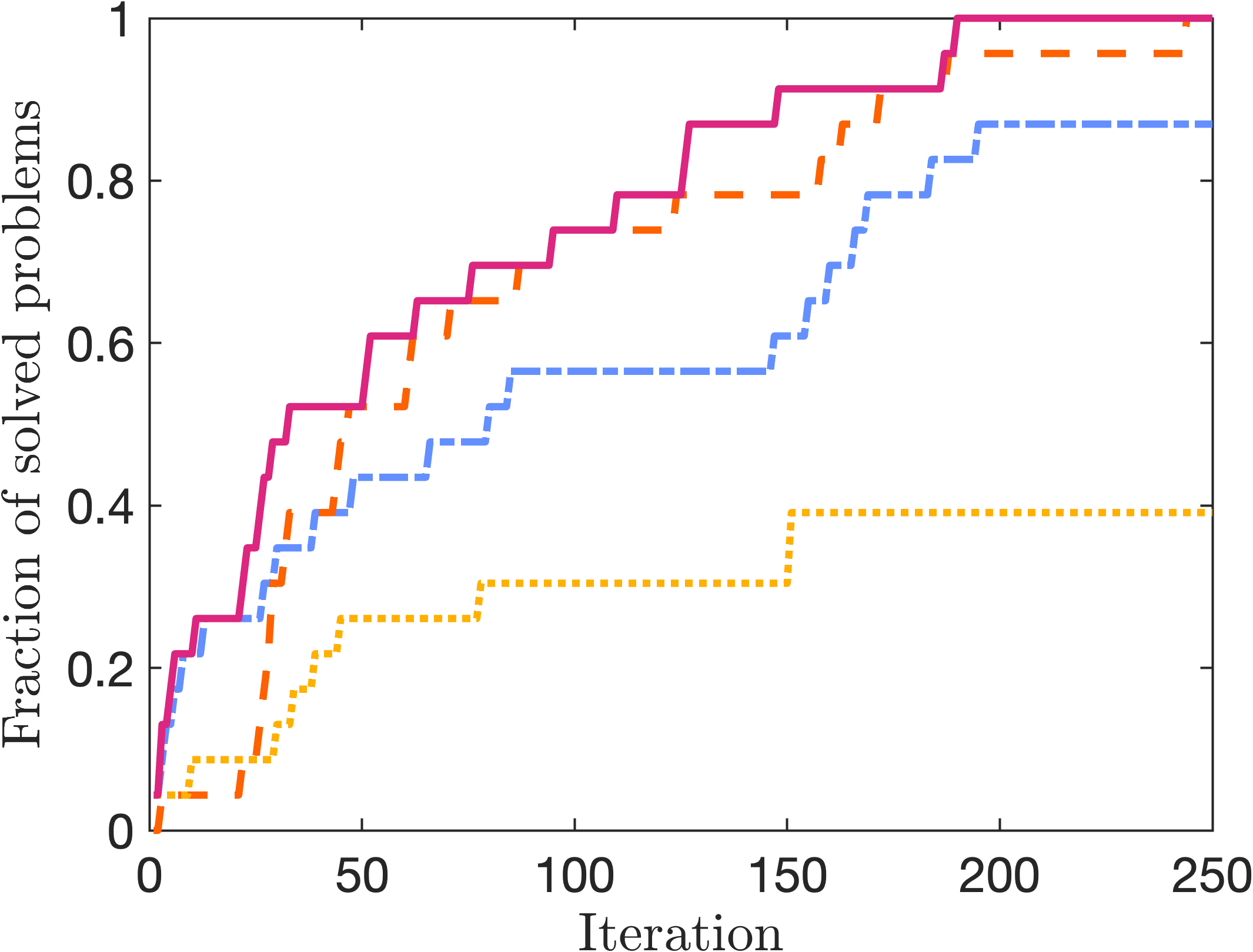
Figure 1: Fraction of solved problems versus number of CG iterations for the 21 KRR problem instances in Table 1.

We compare the RPCholesky method for producing the low-rank approximation $\bm{\widehat{A}}$ with two classic algorithms for partial Cholesky decomposition, greedy pivot selection [19, 40] and uniformly random pivot selection [13, 18]. From the results in Figure 1, we see that RPCholesky improves on both the greedy and uniform pivot selection strategies. Additionally, in several of the 21 KRR problems that we considered, uniform and greedy Nyström preconditioning exhibit failure modes that cause them to converge slowly. In Figure 2 we display two of the runs from Figure 1 with rank $r=500$. In these runs, RPCholesky converges 40$\times$ faster than the uniform method (left panel) and 3$\times$ faster than the greedy method (right panel).

COMET-MC-SAMPLE

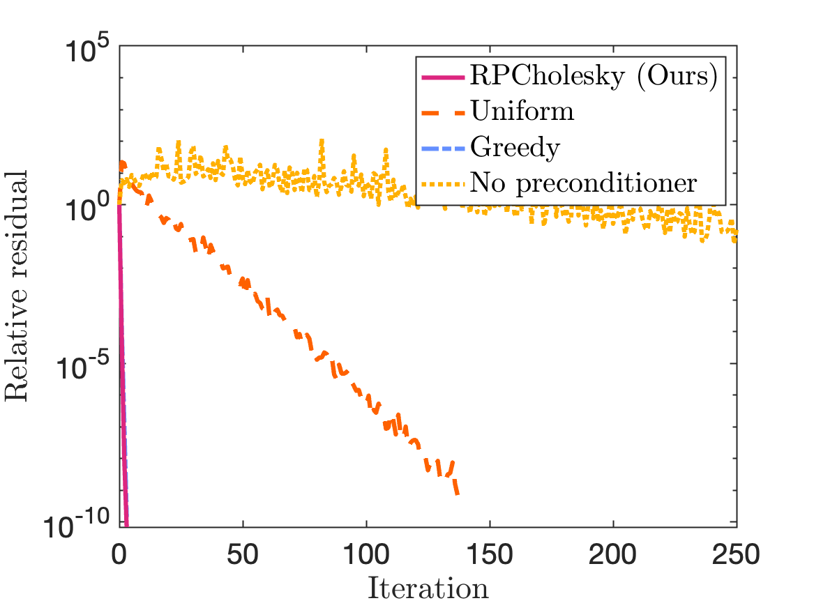
creditcard

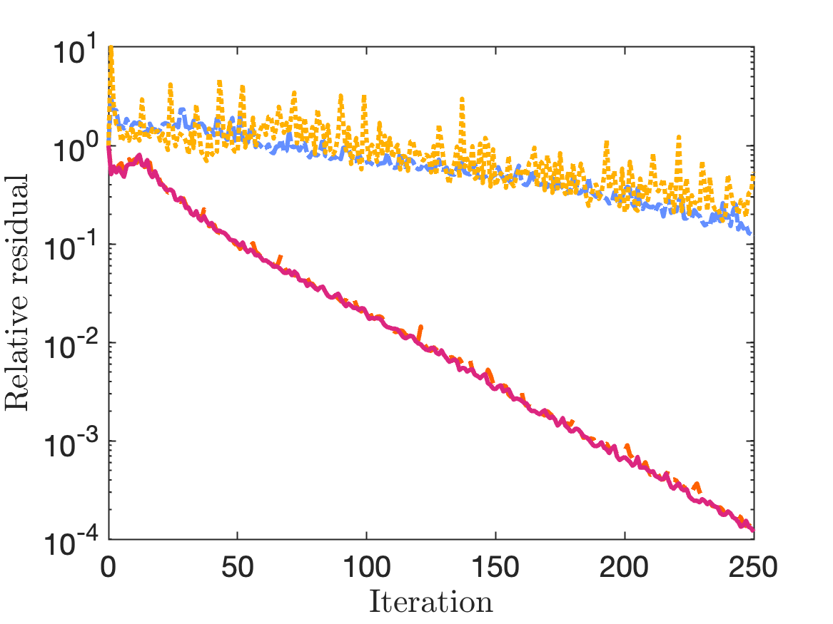
Figure 2: Relative residual versus number of CG iterations for (left) COMET-MC-SAMPLE data and (right) creditcard data. The trajectory of the Greedy method matches almost perfectly the trajectory of RPCholesky on the left panel.

2.1.3 Theoretical guarantees

The sole requirement for RPCholesky’s success is an eigenvalue decay condition which ensures the accuracy of the low-rank approximation $\bm{\widehat{A}}\approx\bm{A}$. To explain this condition in detail, we introduce a quantitative measure of the eigenvalue decay called the $\mu$-tail rank of the matrix $\bm{A}$:

Definition 2.1 (Tail rank).

The $\mu$-tail rank of a psd matrix $\bm{A}\in\mathbb{R}^{N\times N}$ is

$$\textup{rank}_{\mu}(\bm{A}):=\min\Bigl{\{}r\geq 0:\,\sum\nolimits_{i>r}\lambda_{i}(\bm{A})\leq\mu\Bigr{\}}.$$

In typical KRR problems with the squared exponential kernel (2.3), the eigenvalues of the kernel matrix $\bm{A}$ decay exponentially, so we expect that the $\mu$-tail rank may be as small as $\mathcal{O}(\log(1/\mu))$.

Next, we state our main performance guarantee for RPCholesky preconditioning; the proof appears in Section 5.1.

Theorem 2.2 (RPCholesky preconditioning).

Fix a failure probability $\delta\in(0,1)$ and an error tolerance $\varepsilon\in(0,1)$. Let $\bm{A}$ be any positive-semidefinite matrix. Construct a random approximation $\bm{\widehat{A}}$ using RPCholesky with block size $B=1$ and approximation rank

$$r\geq\textup{rank}_{\mu}(\bm{A})\,\bigl{(}1+\log\bigl{(}\operatorname{tr}\bm{A}/\mu\bigr{)}\bigr{)}.$$ (2.4)

With probability at least $1-\delta$ over the randomness in $\bm{\widehat{A}}$, the RPCholesky preconditioner $\bm{P}=\bm{\widehat{A}}+\mu\mathbf{I}$ controls the condition number at a level

$$\kappa\bigl{(}\bm{P}^{-1/2}(\bm{A}+\mu\mathbf{I})\bm{P}^{-1/2}\bigr{)}\leq 3/\delta.$$ (2.5)

Conditional on the event (2.5), when we apply preconditioned CG to the KRR linear system $(\bm{A}+\mu\mathbf{I})\bm{\beta}=\bm{y}$, we obtain an approximate solution $\bm{\beta}^{(t)}$ for which

$$\lVert\bm{\beta}^{(t)}-\bm{\beta}\rVert_{\bm{A}+\mu\mathbf{I}}\leq\varepsilon\cdot\lVert\bm{\beta}\rVert_{\bm{A}+\mu\mathbf{I}}$$ (2.6)

at any iteration $t\geq\delta^{-1/2}\log(2/\varepsilon)$, where $\bm{\beta}$ is the actual solution.

Theorem 2.2 ensures that RPCholesky-preconditioned CG can solve any full-data KRR problem to fixed error tolerance $\varepsilon$ with failure probability $\delta$, provided that the eigenvalue condition (2.4) is satisfied. This eigenvalue condition ensures that the approximation rank $r$ is large enough to reliably capture the large eigenvalues of the kernel matrix. The factor $\log(\operatorname{tr}\bm{A}/\mu)$ is modest in size, being at most $\log\bigl{(}2^{53}\bigr{)}=36.7$ in double-precision arithmetic. Thus, the expression (2.4) is mainly determined by the $\textup{rank}_{\mu}(\bm{A})$ factor, which counts the number of “large” eigenvalues, with the rest of the eigenvalues adding up to size $\mu$ or smaller. The $\mu$-tail rank is size $\mathcal{O}(\sqrt{N})$ if the eigenvalues decay cubically or faster and the regularization parameter is $\mu=\mathcal{O}(1/N)$, or if the eigenvalues decay quadratically or faster and the regularization is $\mu=\mathcal{O}(1/\sqrt{N})$.

If $\textup{rank}_{\mu}(\bm{A})$ is $\mathcal{O}(\sqrt{N})$ and we apply RPCholesky preconditioning with $r=\mathcal{O}(\sqrt{N})$ columns, Theorem 2.2 guarantees that we can solve any full-data KRR problem in $\mathcal{O}(N^{2})$ operations. Uniform and greedy Nyström preconditioning admit no similar guarantee (see Section 3.1). Theorem 2.2 also provides insight into the case where the $\mu$-tail rank is larger than $\mathcal{O}(\sqrt{N})$. In this case, we may need to use a larger approximation rank $r$, and the construction cost for the preconditioner would exceed $\mathcal{O}(N^{2})$ operations.

In practice, the parameter $r$ should be tuned to balance the cost of forming the preconditioner and the cost of the CG iterations. As a simple default, we recommend setting $r=10\sqrt{N}$, which is large enough to ensure that all 21 test problems are solved in fewer than 200 iterations (Figure 1 right panel). See Section 4.1 for more exploration of the parameter $r$ with a larger data set.

2.2 Restricted kernel ridge regression

If the number of data points is so large that we cannot apply full-data KRR, we can pursue an alternative approach that we call “restricted KRR”, which was proposed in [35]. In restricted KRR, we build a prediction function

$$\widehat{f}(\bm{x};\bm{\widehat{\beta}})=\sum\nolimits_{i=1}^{k}\widehat{\beta}_{i}K(\bm{x}^{(s_{i})},\bm{x}),$$

using a subset $\bm{x}^{(s_{1})},\bm{x}^{(s_{2})},\ldots,\bm{x}^{(s_{k})}$ of input points, which are called “centers”. There are many strategies for selecting the centers, such as uniform sampling, ridge leverage score sampling, and RPCholesky. One must balance the computational cost of the center selection procedure against the quality of the centers. For all experiments in this paper, we use the computationally trivial approach of sampling centers uniformly at random; however, the development of fast procedures for identifying high-quality centers is an interesting topic for future work.

In restricted KRR, the coefficients $\bm{\widehat{\beta}}$ are chosen to minimize the loss function

$$L(\bm{\widehat{\beta}})=\lVert\bm{y}-\bm{A}(:,\mathsf{S})\bm{\widehat{\beta}}\rVert^{2}+\mu\bm{\widehat{\beta}}^{\ast}\bm{A}(\mathsf{S},\mathsf{S})\bm{\widehat{\beta}},$$

where $\bm{A}(:,\mathsf{S})$ denotes the submatrix of $\bm{A}$ with column indices in $\mathsf{S}=\{s_{1},\ldots,s_{k}\}$ and $\bm{A}(\mathsf{S},\mathsf{S})$ denotes the submatrix with row and column indices both in $\mathsf{S}$. Minimizing this quadratic loss function leads to a coefficient vector $\bm{\widehat{\beta}}$ that satisfies

$$\bigl{[}\bm{A}(\mathsf{S},:)\bm{A}(:,\mathsf{S})+\mu\bm{A}(\mathsf{S},\mathsf{S})\bigr{]}\,\bm{\widehat{\beta}}=\bm{A}(\mathsf{S},:)\bm{y}.$$ (2.7)

Equation 2.7 is a $k\times k$ linear system, which is smaller than the full-data KRR problem. Yet it is still expensive to solve (2.7) by direct methods because of the $\mathcal{O}(k^{2}N)$ cost of forming $\bm{A}(\mathsf{S},:)\bm{A}(:,\mathsf{S})$. When the number of centers is moderately large ($k\geq 10^{3}$), we recommend a cheaper approach for solving (2.7) using conjugate gradient with the KRILL preconditioner, as described in the next section. We will prove that KRILL preconditioning solves every restricted KRR problem in $\mathcal{O}((N+k^{2})k\log k)$ arithmetic operations (Theorem 2.3).

2.2.1 KRILL preconditioning

Algorithm 2 KRILL preconditioning

1:Positive semidefinite matrix $\bm{A}\in{}^{N\times N}$, right-hand-side vector $\bm{y}\in{}^{N}$, regularization coefficient $\mu$, centers $\mathsf{S}$, and tolerance $\varepsilon$.

2:Approximate solution $\widehat{\bm{\beta}}_{\ast}$ to $(\bm{A}(\mathsf{S},:)\bm{A}(:,\mathsf{S})+\mu\,\bm{A}(\mathsf{S},\mathsf{S}))\bm{\widehat{\beta}}=\bm{A}(\mathsf{S},:)\bm{y}$

3:$k\leftarrow|\mathsf{S}|$.

4:$\bm{\Phi}\leftarrow\textsc{SparseSignEmbedding}(d=2k,N,\zeta=\min\{8,2k\})$ $\triangleright$ See Algorithm 5

5:$\bm{P}\leftarrow(\bm{\Phi}\bm{A}(:,\mathsf{S}))^{\ast}(\bm{\Phi}\bm{A}(:,\mathsf{S}))+\mu\bm{A}(\mathsf{S},\mathsf{S})$

6:$\bm{C}\leftarrow\textsc{Cholesky}(\bm{P}+\varepsilon_{\rm mach}\operatorname{tr}(\bm{P})\cdot\mathbf{I})$ $\triangleright$ $\varepsilon_{\rm mach}\approx 2\times 10^{-16}$ in double precision

7:Define primitives for preconditioned conjugate gradient:

Product $$:\widehat{\bm{\beta}}\mapsto\bm{A}(:,\mathsf{S})(\bm{A}(\mathsf{S},:)\bm{\widehat{\beta}})+\mu\cdot\bm{A}(\mathsf{S},\mathsf{S})\widehat{\bm{\beta}}$$

Preconditioner $$:\widehat{\bm{\beta}}\mapsto\bm{C}^{-1}(\bm{C}^{-\ast}\widehat{\bm{\beta}})$$

8:$\bm{\widehat{\beta}}_{\star}\leftarrow\textsc{PCG}(\texttt{Product},\bm{A}(\mathsf{S},:)\bm{y},\varepsilon,\texttt{Preconditioner})$ $\triangleright$ See Algorithm 3

The KRILL preconditioner is based on a randomized approximation of the Gram matrix $\bm{G}=\bm{A}(\mathsf{S},:)\bm{A}(:,\mathsf{S})$. To form this approximation, we generate a sparse random sign embedding [24, §9.2]:

$$\bm{\Phi}=\tfrac{1}{\sqrt{\zeta}}\begin{bmatrix}\bm{\phi}_{1}&\cdots&\bm{\phi}_{N}\end{bmatrix}\in{}^{d\times N},$$

where $\bm{\phi}_{1},\ldots,\bm{\phi}_{N}$ are sparse columns that possess uniform $\pm 1$ values in $\zeta$ uniformly randomly chosen positions. For appropriate parameters, we find that $\bm{\Phi}^{\ast}\bm{\Phi}\approx\mathbf{I}$ in the spectral sense, and we can approximate the Gram matrix as $\bm{\widehat{G}}=\bm{A}(\mathsf{S},:)\bm{\Phi}^{\ast}\bm{\Phi}\bm{A}(:,\mathsf{S})$. This motivates the construction of the KRILL preconditioner

$$\bm{P}=\bm{A}(\mathsf{S},:)\bm{\Phi}^{\ast}\bm{\Phi}\bm{A}(:,\mathsf{S})+\mu\bm{A}(\mathsf{S},\mathsf{S}).$$ (2.8)

We provide pseudocode for KRILL preconditioning in Algorithm 2.

KRILL preconditioning is efficient because we can evaluate $\bm{\widehat{G}}$ in fewer operations than evaluating the Gram matrix $\bm{G}$, with the precise number of operations depending on the sparsity $\zeta$ and the embedding dimension $d$. In our theoretical analysis, we assume $\zeta=\mathcal{O}(\log k)$ and $d=\mathcal{O}(k\log k)$, and we can form $\bm{\widehat{G}}$ in $\mathcal{O}((N+k^{2})k\log k)$ operations. In practice, however, we still observe fast CG convergence when we use a smaller, sparser embedding with $\zeta=\min\{8,2k\}$ and $d=2k$ [37, p. A2440]. Consequently, after including the cost of the CG iterations, the total operating cost of KRILL preconditioning is $\mathcal{O}((N+k^{2})k\log k)$ in theory and $\mathcal{O}((N+k^{2})k)$ in practice.

2.2.2 Empirical performance

Figure 3 compares KRILL with the current state-of-the-art FALKON preconditioner across the 21 regression and classification problems described in Table 1. For each problem, we subsample $N=4\times 10^{4}$ data points and select either $k=200=\sqrt{N}$ (left) or $k=4000=N/10$ (right) centers uniformly at random. We then standardize the features and apply KRR with a squared exponential kernel (2.3) using the parameters $\sigma=3$ and $\mu/N=10^{-7}$. We run $100$ CG iterations and declare a problem to be “solved” if the relative residual

$$\frac{\lVert\bigl{[}\bm{A}(\mathsf{S},:)\bm{A}(:,\mathsf{S})+\mu\bm{A}(\mathsf{S},\mathsf{S})\bigr{]}\bm{\widehat{\beta}}-\bm{A}(\mathsf{S},:)\bm{y}\rVert}{\lVert\bm{A}(\mathsf{S},:)\bm{y}\rVert}$$

falls below a tolerance of $\varepsilon=10^{-4}$.

Fewer centers: $k=200=\sqrt{N}$

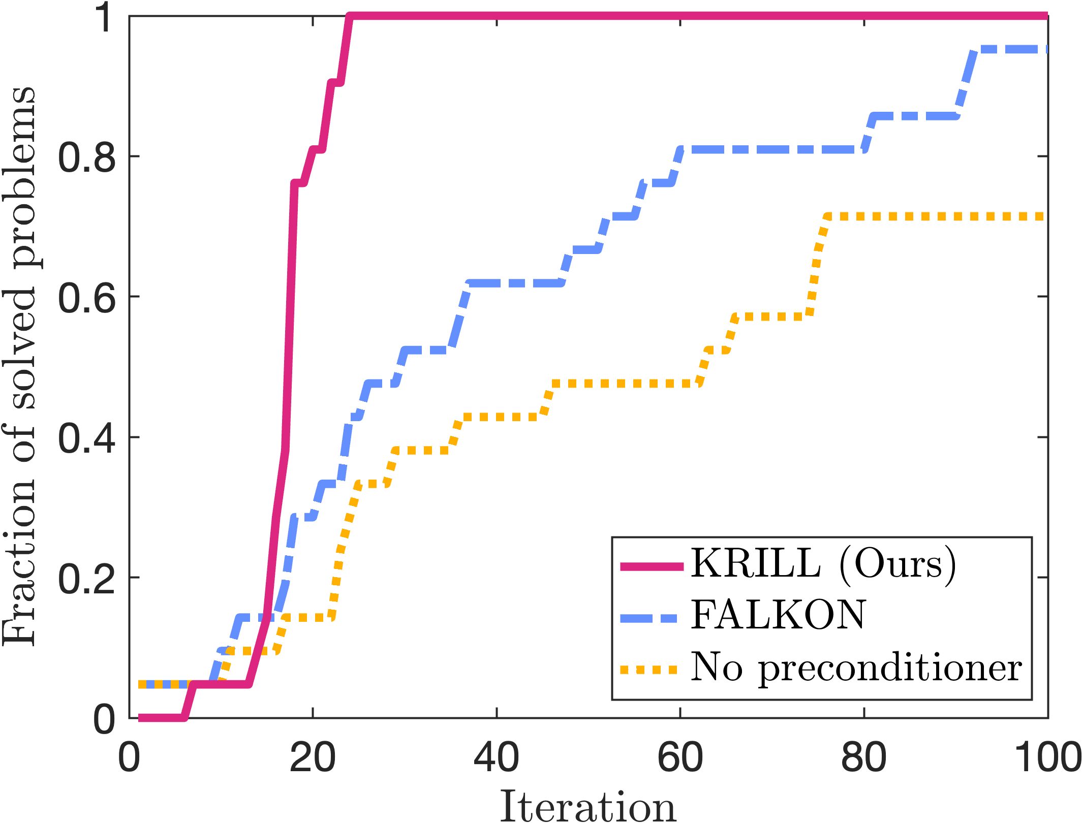
More centers: $k=4000=N/10$

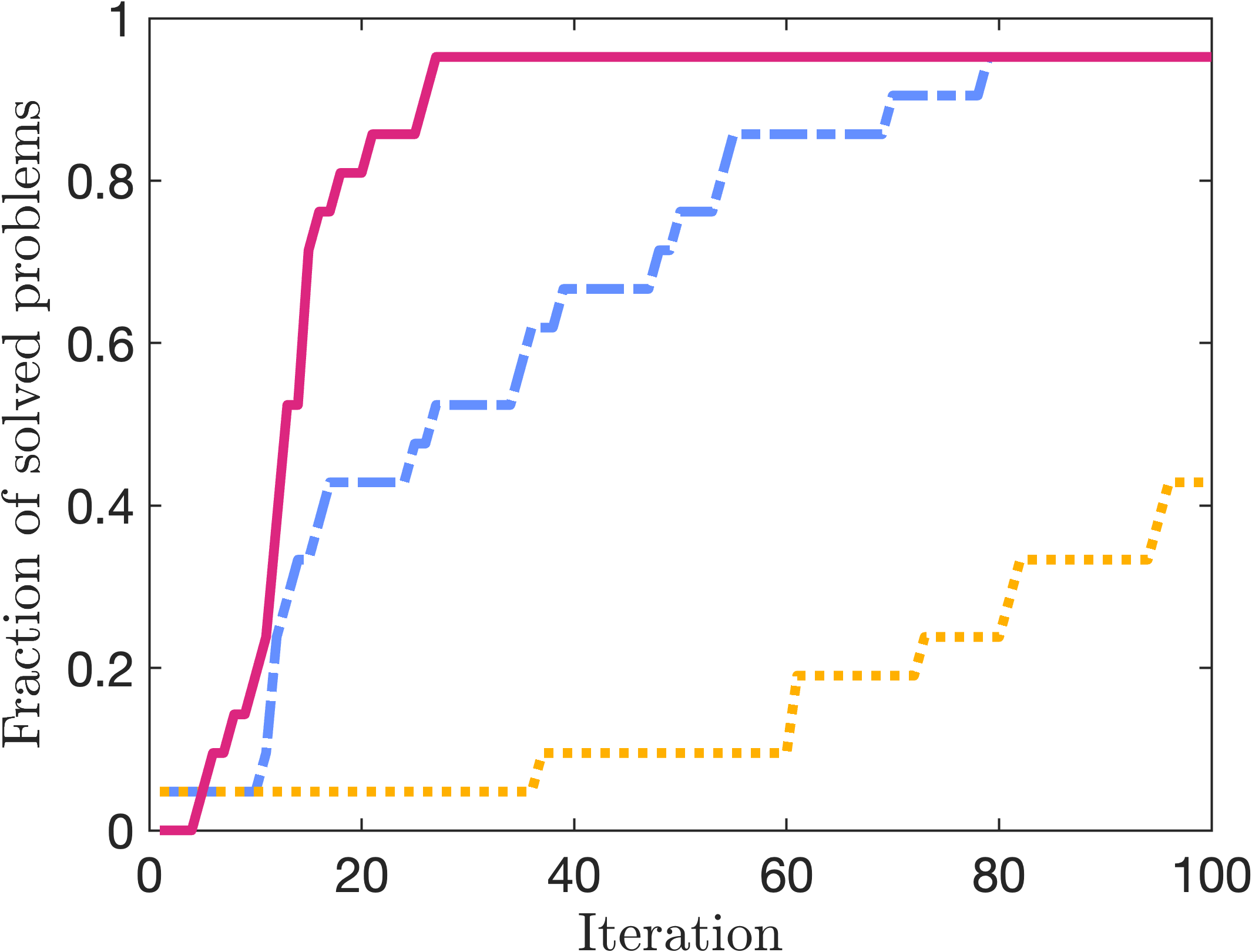
Figure 3: Fraction of solved problems versus number of CG iterations for the 21 kernel problems in Table 1.

Examining Figure 3, we find that KRILL solves many more problems than FALKON. The greatest difference arises in the small $k$ regime (left). After just 25 iterations, KRILL solves all of the classification and regression problems, whereas FALKON only solves half of them. In the large $k$ regime (right), KRILL solves all but one problem after $30$ iterations: this problem is extremely ill-conditioned to the point of causing numerical issues in finite-precision arithmetic.

As a typical example, Figure 4 displays the performance of KRILL and FALKON applied to the HIGGS classification data set, either with few centers $k=200$ (left) and many centers $k=4000$ (right). KRILL improves on FALKON’s performance by exhibiting fast convergence regardless of the number of centers. As we shall see in Section 4.2, KRILL also improves the runtime.

Fewer centers: $k=200=\sqrt{N}$

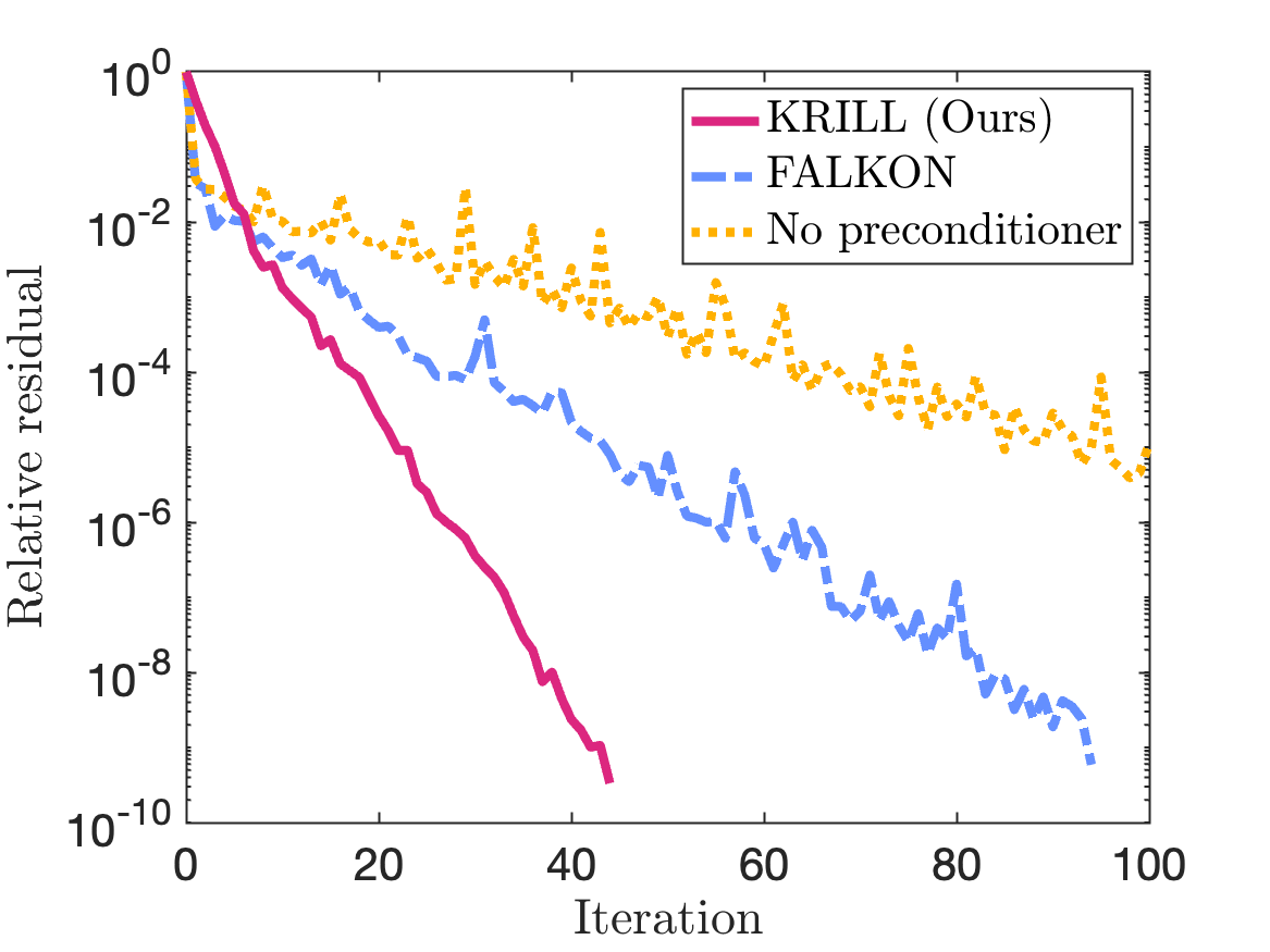
More centers: $k=4000=N/10$

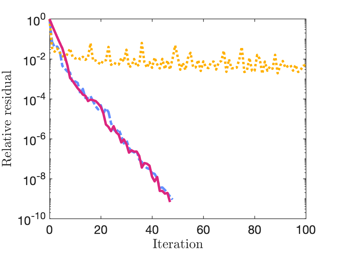
Figure 4: Relative residual versus number of CG iterations for HIGGS with (left) $200$ centers and (right) $4000$ centers.

2.2.3 Theoretical guarantees

With the proper parameter choices, KRILL is guaranteed to solve any restricted KRR problem with any positive-semidefinite kernel matrix $\bm{A}\in{}^{N\times N}$ and any regularization parameter $\mu>0$. Here, we state our main guarantee for KRILL, which is established in Section 5.2.

Theorem 2.3 (KRILL performance guarantee).

Fix a failure probability $\delta\in(0,1)$ and an error tolerance $\varepsilon\in(0,1)$. Let $\bm{A}$ be any positive-semidefinite matrix; let $\mathsf{S}$ be an index set of cardinality $|\mathsf{S}|=k$; and define $\bm{M}=\bm{A}(\mathsf{S},:)\bm{A}(:,\mathsf{S})+\mu\bm{A}(\mathsf{S},\mathsf{S})$. Draw a random sparse sign embedding $\bm{\Phi}\in{}^{d\times N}$ with column sparsity $\zeta$ and embedding dimension $d$ satisfying

$$\zeta=\Theta(\log(k/\delta))\quad\text{and}\quad d=\Theta(k\log(k/\delta)).$$ (2.9)

With probability at least $1-\delta$ over the randomness in $\bm{\Phi}$, the KRILL preconditioner $\bm{P}=\bm{A}(\mathsf{S},:)\bm{\Phi}^{\ast}\bm{\Phi}\bm{A}(:,\mathsf{S})+\mu\bm{A}(\mathsf{S},\mathsf{S})$ controls the condition number at a level

$$\kappa\bigl{(}\bm{P}^{-1/2}\bm{M}\bm{P}^{-1/2}\bigr{)}\leq 3.$$ (2.10)

Conditional on the event (2.10), when we apply preconditioned CG to the linear system $\bm{M}\widehat{\bm{\beta}}=\bm{A}(\mathsf{S},:)\bm{y}$, we obtain an approximate solution $\widehat{\bm{\beta}}^{(t)}$ for which

$$\lVert\widehat{\bm{\beta}}^{(t)}-\widehat{\bm{\beta}}\rVert_{\bm{M}}\leq\varepsilon\lVert\widehat{\bm{\beta}}\rVert_{\bm{M}},$$ (2.11)

at any iteration $t\geq\log(2/\varepsilon)$, where $\widehat{\bm{\beta}}$ is the actual solution.

Theorem 2.3 implies that KRILL can solve any restricted KRR problem in $\mathcal{O}((N+k^{2})k\log k)$ operations (in exact precision arithmetic). In contrast, FALKON-type preconditioners [32, 25, 33] are only guaranteed to solve restricted KRR problems if the number of centers and regularization satisfy $k=\Omega(\sqrt{N})$ and $\mu=\Omega(\sqrt{N})$ [32, 33]. Given these constraints, it is no surprise that KRILL performs more robustly than FALKON in our experiments.

3 Background and comparisons with other preconditioners

In this section, we compare our new preconditioners with existing preconditioners for solving the full-data and restricted KRR equations. To begin, we observe that the full-data and restricted KRR equations both take the form

$$\bm{M}\bm{z}=\bm{b},$$ (3.1)

where $\bm{M}\in{}^{d\times d}$ is a positive-definite matrix and $\bm{b}\in{}^{d}$ is a vector. In full-data KRR, the dimension $d$ equals the number of data points, $d=N$. In restricted KRR, the dimension equals the number of data centers, $d=k$.

Preconditioned conjugate gradient

The conjugate gradient (CG) algorithm [34, §6.7] is a popular approach for solving linear systems of the form (3.1). When $\bm{M}$ is well-conditioned ($\kappa(\bm{M})\approx 1$), CG gives a high-accuracy solution using only a small number of iterations, where each iteration requiring a matrix–vector product with $\bm{M}$. More precisely, the following bound [34, eq. (6.128)] controls the convergence rate of the CG iterates $\bm{z}^{(0)},\bm{z}^{(1)},\ldots$ to the solution $\bm{z}$ of the system (3.1):

$$\left\|\smash{\bm{z}^{(t)}-\bm{z}}\right\|_{\bm{M}}\leq 2\Biggl{(}\frac{\sqrt{\kappa(\bm{M})}-1}{\sqrt{\kappa(\bm{M})}+1}\Biggr{)}^{t}\left\|\smash{\bm{z}^{(0)}-\bm{z}}\right\|_{\bm{M}},$$ (3.2)

The convergence is exponentially fast in the $\bm{M}$-norm $\lVert\bm{v}\rVert_{\bm{M}}:=(\bm{v}^{\ast}\bm{M}\bm{v})^{1/2}$. However, the exponential rate depends on the condition number $\kappa(\bm{M})$, and it can be slow when $\kappa(\bm{M})$ is large.

The full-data and restricted KRR equations are typically ill-conditioned, so we need to apply a positive-definite preconditioner $\bm{P}\in{}^{d\times d}$ to these problems to improve the convergence. The preconditioned CG algorithm (Algorithm 3, described in [20, §10.3]), is equivalent to applying standard CG to the preconditioned system

$$\bigl{(}\bm{P}^{-1/2}\bm{M}\bm{P}^{-1/2}\bigr{)}\bigl{(}\bm{P}^{1/2}\bm{z}\bigr{)}=\bm{P}^{-1/2}\bm{b}.$$

The convergence rate of preconditioned CG no longer depends on $\kappa(\bm{M})$, instead depending on $\kappa(\bm{P}^{-1/2}\bm{M}\bm{P}^{-1/2})$. Thus, we have fast convergence when $\bm{P}\approx\bm{M}$.

Algorithm 3 Preconditioned conjugate gradient

1:Subroutine Product computing the action $\bm{u}\mapsto\bm{M}\bm{u}$, subroutine Preconditioner computing the action $\bm{u}\mapsto\bm{P}^{-1}\bm{u}$, right-hand-side vector $\bm{b}\in{}^{N}$, and tolerance $\varepsilon$.

2:Approximate solution $\bm{\beta}_{\star}$ to $\bm{M}\bm{\beta}=\bm{b}$.

3:Initialize $\bm{\beta}_{\star}\leftarrow\bm{0},\>\bm{r}\leftarrow\bm{b},\>\bm{z}\leftarrow\texttt{Preconditioner}(\bm{r}),\>\bm{p}\leftarrow\bm{z},$ and $\omega\leftarrow\bm{z}^{*}\bm{r}$

4:while $\|\bm{r}\|\geq\varepsilon\cdot\left\|\bm{b}\right\|$ do

5:     $\bm{v}\leftarrow\texttt{Product}(\bm{p})$

6:     $\eta\leftarrow\omega/\bm{v}^{*}\bm{p}$, $\bm{\beta}_{\star}\leftarrow\bm{\beta}_{\star}+\eta\bm{p}$, $\bm{r}\leftarrow\bm{r}-\eta\bm{v}$

7:     $\bm{z}\leftarrow\texttt{Preconditioner}(\bm{r})$

8:     $\omega_{\rm new}\leftarrow\bm{z}^{*}\bm{r},\gamma\leftarrow\omega_{\rm new}/\omega,\omega\leftarrow\omega_{\rm new}$

9:     $\bm{p}\leftarrow\bm{z}+\gamma\bm{p}$

10:end while

In the rest of this section, we review the history of preconditioned CG methods for the full-data and restricted KRR equations. We do not cover KRR methods based on sketch-and-solve [5, 1] or stochastic gradient descent [14, 23], since the accuracy of these methods is more limited [24, §10].

3.1 Preconditioners for full-data KRR

To efficiently solve the full-data KRR problem $(\bm{A}+\mu\mathbf{I})\bm{x}=\bm{y}$, we can apply a preconditioner of the form

$$\bm{P}=\bm{\widehat{A}}+\mu\mathbf{I},$$

where $\bm{\widehat{A}}\in{}^{N\times N}$ is an approximation of the full kernel matrix $\bm{A}$. Ideally, we should have an accurate approximation $\bm{\widehat{A}}\approx\bm{A}$, and we should be able to quickly apply $\bm{P}^{-1}$ to a vector at every CG step.

In the KRR literature, $\bm{\widehat{A}}$ is typically constructed as a low-rank approximation of $\bm{A}$ [13, 4, 19, 40, 18]. A low-rank approximation can only be accurate when the kernel matrix is close to being low-rank, i.e., when the eigenvalues of $\bm{A}$ decay quickly. However, even under favorable eigenvalue decay conditions, it has been a challenge to identify accurate and computationally tractable low-rank approximations.

A popular low-rank approximation method for KRR problems is the column Nyström approximation [24, §19.2], which is obtained from a partial Cholesky decomposition with pivoting. The column Nyström approximation takes the form

$$\bm{\widehat{A}}=\bm{A}(:,\textsf{S})\bm{A}(\textsf{S},\textsf{S})^{\dagger}\bm{A}(\textsf{S},:),$$ (3.3)

where $\textsf{S}=\{s_{1},s_{2},\ldots,s_{r}\}$ coincides with the pivots chosen in the Cholesky procedure, and it lists the columns of $\bm{A}$ that participate in the approximation. The column Nyström approximation is convenient because it is formed from the columns of $\bm{A}$ indexed by S and does not require viewing the rest of the matrix. Yet the accuracy of the column Nyström approximation depends on selecting a good index set $\mathsf{S}$. In the context of full-data KRR, there are two prominent strategies for picking the set $\mathsf{S}$ of columns in the Nyström approximation, called uniform sampling and greedy selection. Both of these approaches exhibit serious failure modes.

Failure of uniform sampling

The first strategy selects the column pivots $s_{1},\ldots,s_{r}$ uniformly at random [13, 18]. This uniform sampling method can be effective for some problems, but it fails to explore less populated regions of data space. To illustrate this shortcoming, let $\bm{1}_{m}$ denote the $m$-vector with entries equal to $1$, and consider the kernel matrix

$$\bm{A}=\begin{pmatrix}\bm{1}_{N-N^{1/3}}^{\vphantom{*}}\bm{1}_{N-N^{1/3}}^{\ast}&~{}\\ ~{}&\bm{1}_{N^{1/3}}^{\vphantom{*}}\bm{1}_{N^{1/3}}^{\ast}\end{pmatrix}.$$

In principle, constructing a preconditioner for $\bm{A}$ should be easy, since the $\mu$-tail rank (Definition 2.1) is just $\textup{rank}_{\mu}(\bm{A})=2$ for any $\mu<N^{1/3}$. However, uniform sampling selects many columns from the left block and neglects columns from the right block that are also needed to ensure the approximation quality. For uniform sampling to build an effective preconditioner, we need an approximation rank much higher than $2$ and at least as large as $r=\Omega(N^{2/3})$.

Failure of greedy selection

A second strategy for choosing columns is the greedy selection method [19, 40], in which we adaptively select each column pivot $s_{i}$ by finding to the largest diagonal element of the residual matrix $\bm{A}-\bm{\widehat{A}}_{(i-1)}$ after $i-1$ steps of the Cholesky procedure. The greedy method has the opposite failure mode from the uniform method: it focuses on outlier data points and fails to explore highly populated regions of data space. To see this limitation, let $\mathbf{I}_{m}$ denote the $m\times m$ identity matrix, and consider the kernel matrix

$$\bm{A}=\bm{1}_{N}^{\vphantom{\ast}}\bm{1}_{N}^{\ast}+\begin{pmatrix}\frac{\delta}{2}\,\bm{1}_{N-N^{2/3}}^{\vphantom{*}}\bm{1}_{N-N^{2/3}}^{\ast}&~{}\\ &\delta\,\mathbf{I}_{N^{2/3}}\end{pmatrix}$$

for a small parameter $\delta>0$. Constructing a preconditioner for $\bm{A}$ is easy in theory, since $\textup{rank}_{\mu}(\bm{A})\leq 2$ for any $\mu\geq N^{2/3}\delta$. Yet the greedy strategy selects columns from the right block first and misses the left columns. For greedy sampling to provide an effective preconditioner, we need an approximation rank $r>N^{2/3}$, which is large enough that all the columns in the right block have been selected.

Algorithm 4 Blocked RPCholesky for psd low-rank approximation

1:Positive semidefinite matrix $\bm{A}\in{}^{N\times N}$, approximation rank $k$, block size $B$.

2:Factor matrix $\bm{F}\in{}^{N\times k}$, index set $\mathsf{S}$.

3:Initialize $\bm{F}\leftarrow\bm{0}_{N\times k}$, $\mathsf{S}\leftarrow\emptyset$, $\bm{d}\leftarrow\operatorname{diag}(\bm{A})$, $i\leftarrow 0$

4:while $i<k$ do

5:     Sample iid indices $s_{1},\dots,s_{\min\{B,k-i\}}\sim\bm{d}/\textsc{Sum}(\bm{d})$

6:     $\mathsf{S}^{\prime}\leftarrow\textsc{Unique}(s_{1},\dots,s_{\min\{B,k-i\}})$, $\mathsf{S}\leftarrow\mathsf{S}\cup\mathsf{S}^{\prime}$

7:     $\bm{G}\leftarrow\bm{A}(:,\mathsf{S}^{\prime})-\bm{F}(:,1:i)\bm{F}(\mathsf{S}^{\prime},1:i)^{*}$

8:     $\bm{R}\leftarrow\textsc{Cholesky}(\bm{G}(\mathsf{S}^{\prime},:))$ $\triangleright$ $\bm{G}(\mathsf{S}^{\prime},:)=\bm{R}^{*}\bm{R}$

9:     $\bm{F}\left(:,(i+1):(i+|\mathsf{S}^{\prime}|)\right)\leftarrow\bm{G}\bm{R}^{-1}$

10:     $\bm{d}\leftarrow\bm{d}-\textsc{SquaredRowNorms}\left(\bm{F}\left(:,(i+1):(i+|\mathsf{S}^{\prime}|)\right)\right)$

11:     $i\leftarrow i+|\mathsf{S}^{\prime}|$

12:end while

Advantages of RPCholesky

In this paper, we propose a new KRR preconditioner that uses RPCholesky (see Algorithm 4 or [10]) to select the columns for the Nyström approximation. In RPCholesky, we adaptively sample the column pivot $s_{i}$ with probability proportional to the diagonal entries of the residual matrix $\bm{A}-\bm{\widehat{A}}_{(i-1)}$ after $i-1$ steps of the Cholesky procedure. Because of the adaptive sampling distribution, RPCholesky balances exploration of the small diagonal entries and exploitation of the large diagonal entries, avoiding the failure modes of both the uniform and greedy strategies. RPCholesky is guaranteed to produce an effective preconditioner if the approximation rank $r$ is set to a modest multiple of the $\mu$-tail rank (Theorem 2.2).

More expensive Gaussian preconditioner

A different type of preconditioner for full-data KRR is based on the Gaussian Nyström approximation [18]

$$\bm{\widehat{A}}=\bm{A}\bm{X}(\bm{X}^{*}\bm{A}\bm{X})^{\dagger}\bm{X}^{*}\bm{A},$$

where $\bm{X}\in{}^{N\times r}$ is a matrix with independent standard normal entries. Forming the Gaussian Nyström approximation requires $r$ matrix–vector multiplications with the full kernel matrix, which is much more expensive than forming a column Nyström approximation (3.3) in factored form. Consequently, to achieve a cost of $\mathcal{O}(N^{2})$ operations, we can only afford Gaussian Nyström with a constant approximation rank $r=\mathcal{O}(1)$, whereas we can run RPCholesky preconditioning with a larger approximation rank $r=\mathcal{O}(\sqrt{N})$. Because of this larger approximation rank, RPCholesky preconditioning leads to a more accurate approximation with stronger theoretical guarantees.

Other approaches

We briefly mention two other types of approximations $\bm{\widehat{A}}$ that can be used to build preconditioners for the full-data KRR problem. First, certain types of kernel matrices can be approximated using random features [13, 4], but the quality of the approximation tends to be poor. Numerical tests indicate that the random features approach does not yield a competitive preconditioner [13, 42]. Second, the kernel matrix can also be approximated using a hierarchical low-rank approximation [13, 2, 9, 43]. The hierarchical approach has mainly been applied to low-dimensional input data, and the applicability to high-dimensional data sets remains unclear [2].

3.2 Preconditioners for restricted KRR

To efficiently solve the restricted KRR problem $\bigl{[}\bm{A}(\mathsf{S},:)\bm{A}(:,\mathsf{S})+\mu\bm{A}(\mathsf{S},\mathsf{S})\bigr{]}\,\bm{\widehat{\beta}}=\bm{A}(\mathsf{S},:)\bm{y}$, we can apply a preconditioner of the form

$$\bm{P}=\bm{\widehat{G}}+\mu\bm{A}(\mathsf{S},\mathsf{S}).$$ (3.4)

where $\bm{\widehat{G}}\in{}^{k\times k}$ approximates the Gram matrix $\bm{G}=\bm{A}(\mathsf{S},:)\bm{A}(:,\mathsf{S})$.

FALKON, the current state-of-the-art

FALKON-type preconditioners [32, 33, 25] are based on a Monte Carlo approximation of $\bm{G}$. The approach assumes that each data point $\bm{x}^{(i)}$ is selected as a center with nonzero probability $p_{i}=\mathbb{P}\{i\in\mathsf{S}\}$. The Gram matrix is then approximated as

$$\bm{\widehat{G}}=\bm{A}(\mathsf{S},\mathsf{S})\bm{P}(\mathsf{S},\mathsf{S})^{-1}\bm{A}(\mathsf{S},\mathsf{S}),$$ (3.5)

where $\bm{P}=\operatorname{diag}(p_{1},p_{2},\ldots,p_{N})$ is the diagonal matrix of the selection probabilities. The matrix entries $g_{ij}$ and $\widehat{g}_{ij}$ can be explicitly written as

$$g_{ij}=\sum_{\ell=1}^{N}a_{s_{i},\ell}a_{\ell,s_{j}}\quad\text{and}\quad\widehat{g}_{ij}=\sum_{\ell=1}^{N}\frac{\mathbb{1}\{\ell\in\mathsf{S}\}}{p_{\ell}}a_{s_{i},\ell}a_{\ell,s_{j}}.$$

These entries are clearly linked together in expectation:

$$\sum_{\ell=1}^{N}a_{i,\ell}a_{\ell,j}=\mathbb{E}\Biggl{[}\sum_{\ell=1}^{N}\frac{\mathbb{1}\{\ell\in\mathsf{S}\}}{p_{\ell}}a_{i,\ell}a_{\ell,j}\Biggr{]}\quad\text{for fixed indices $1\leq i,j\leq N$,}$$

which suggests that the quantities $g_{ij}$ and $\widehat{g}_{ij}$ will be close under appropriate conditions. FALKON [32, 25] is a special case of (3.5) in which the centers are sampled uniformly at random, and FALKON-BLESS [33] is a special case of (3.5) in which the centers are chosen by ridge leverage score sampling.

The main limitation of FALKON-type preconditioners is that the Monte Carlo approximation error can be large. To account for the Monte Carlo error, the available analyses [32, 33] assume a large number of centers $k=\Omega(\sqrt{N})$ and a large regularization $\mu=\Omega(\sqrt{N})$. When these assumptions are satisfied, FALKON-type preconditioners solve the restricted KRR equations in $\mathcal{O}((N+k^{2})k)$ operations. However, the assumptions on $k$ and $\mu$ may not be satisfied in practice. For example, $\mu$ is often small when chosen by cross-validation, and [32] contains examples of $\mu$ values up to five orders of magnitude smaller than $\mu=\sqrt{N}$.

Algorithm 5 Sparse sign embedding

1:Embedding dimension $d$, input dimension $N$, sparsity level $\zeta$.

2:Embedding matrix $\bm{\Phi}\in{}^{d\times N}$ in sparse (e.g., CSR) format.

3:$\mathtt{rows}\leftarrow\bm{0}_{\zeta N},\mathtt{cols}\leftarrow\bm{0}_{\zeta N},\mathtt{vals}\leftarrow\bm{0}_{\zeta N}$

4:for $1\leq j\leq N$ do

5:     $\mathtt{rows}((j-1)\zeta+1:j\zeta)\leftarrow$ distinct uniformly random indices from $\{1,\ldots,d\}$

6:     $\mathtt{cols}((j-1)\zeta+1:j\zeta)\leftarrow j$

7:     $\mathtt{vals}((j-1)\zeta+1:j\zeta)\leftarrow\zeta^{-1/2}\cdot\textsc{Unif}\{\pm 1\}^{\zeta}$

8:end for

9:$\bm{\Phi}\leftarrow\textsc{Sparse}(\mathtt{rows},\mathtt{cols},\mathtt{vals},d,N)$ $\triangleright$ $d\times N$ sparse matrix with specified entries

KRILL

In this paper, we recommend using the more accurate KRILL approximation,

$$\bm{\widehat{G}}=\bm{A}(\mathsf{S},:)\bm{\Phi}^{\ast}\bm{\Phi}\bm{A}(:,\mathsf{S}),$$

where $\bm{\Phi}\in{}^{d\times N}$ is a sparse random sign embedding (see Algorithm 5 or [12]). With this approximation, we can guarantee the effectiveness of the KRILL preconditioner $\bm{P}=\bm{\widehat{G}}+\mu\bm{A}(\mathsf{S},\mathsf{S})$, regardless of the number of centers $k$ and the regularization $\mu$.

KRILL is inspired by the sketch-and-precondition approach for solving overdetermined least-squares problems [24, §10.5]. In sketch and precondition, we use a random embedding to approximate the matrix appearing in the normal equations, and the approximate matrix serves as a preconditioner for solving the least-squares problem. Sketch-and-precondition was first proposed in [30] and later refined in [3, 27, 11, 21, 26]. It has been applied with several different embeddings [24, §§8–9], but the empirical comparisons of [16, Fig. 1] suggest the sparse sign embedding is the most efficient. KRILL differs from classical sketch-and-precondition because the embedding is applied to the Gram matrix term $\bm{A}(:,\mathsf{S})\bm{A}(\mathsf{S},:)$ but not the regularization term $\mu\bm{A}(\mathsf{S},\mathsf{S})$. Even so, KRILL is motivated by the same random embedding ideas and its analysis follows the same pattern as sketch-and-precondition.

4 Case studies

In this section, we apply our preconditioning strategies to two scientific applications. In Section 4.1, we apply full-data KRR with RPCholesky preconditioning to predict the chemical properties of a wide range of molecules. In Section 4.2, we apply restricted KRR with KRILL preconditioning to distinguish exotic particle collisions from a background process.

4.1 HOMO energy prediction

A major goal of chemical machine learning is to search over a large parameter space of molecules and identify candidate molecules which may possess useful properties [15, 41]. To support this goal, scientists have assembled the QM9 data set, which describes the properties of $1.3\times 10^{5}$ organic molecules [29, 31]. Although the QM9 data set is generated by relatively expensive (and highly repetitive) density functional theory calculations, we can use the QM9 data to train machine learning models that efficiently make out-of-sample predictions, limiting the need for density functional theory in the future. Ideally, machine learning would identify a small collection of promising molecules, which scientists could then analyze and test.

A recent journal article [36], which was selected as an Editor’s Pick in the Journal of Chemical Physics, describes the difficulties in applying KRR to the QM9 data set. The authors aim to predict the highest-occupied-molecular-orbital (HOMO) energy. In their simplest approach, they make HOMO predictions based on the Coulomb matrix representation of molecules, which is a set of features based on the distances between the atomic nuclei and the nuclear charges. After defining the features, they standardize the features and apply an $\ell_{1}$ Laplace kernel

$$K(\bm{x},\bm{x}^{\prime})=\exp\bigl{(}-\tfrac{1}{\sigma}\lVert\bm{x}-\bm{x}^{\prime}\rVert_{\ell_{1}}\bigr{)},$$

with a bandwidth $\sigma$ and a ridge parameter $\mu$ chosen using cross-validation.

Given the moderate size of the QM9 data set ($N=1.3\times 10^{5}$), it takes just a few seconds to load the data and form individual columns of the kernel matrix. However, on a laptop-scale computer (64GB RAM), there is not enough working memory to store or factorize the complete kernel matrix. The authors of [36] address these computational constraints by randomly subsampling $N=32,000$ or fewer data points and applying full-data KRR to the random sample. In their Fig. 8, they show that the predictive accuracy improves by a factor of $2\times$ as they increase the size of the data from $N=1,000$ to $N=32,000$ data points. Even with $N=32,000$ data points, the predictive accuracy does not saturate, and thus computational constraints are limiting the the predictive accuracy of the KRR model.

Building on this work, we can apply KRR to the complete QM9 data set either using (i) restricted KRR or (ii) full-data KRR with RPCholesky preconditioning. In all our experiments, we split the data into $N=10^{5}$ training points and $M=3\times 10^{4}$ test points, and we measure the predictive accuracy using the symmetric mean absolute percentage error (SMAPE):

$$\operatorname{SMAPE}(\bm{\widehat{y}},\bm{y})=\frac{1}{M}\sum_{i=1}^{M}\frac{|\widehat{y}_{i}-y_{i}|}{(|\widehat{y}_{i}|+|y_{i}|)/2}.$$ (4.1)

The results are presented in Figures 5, 6, and 7.

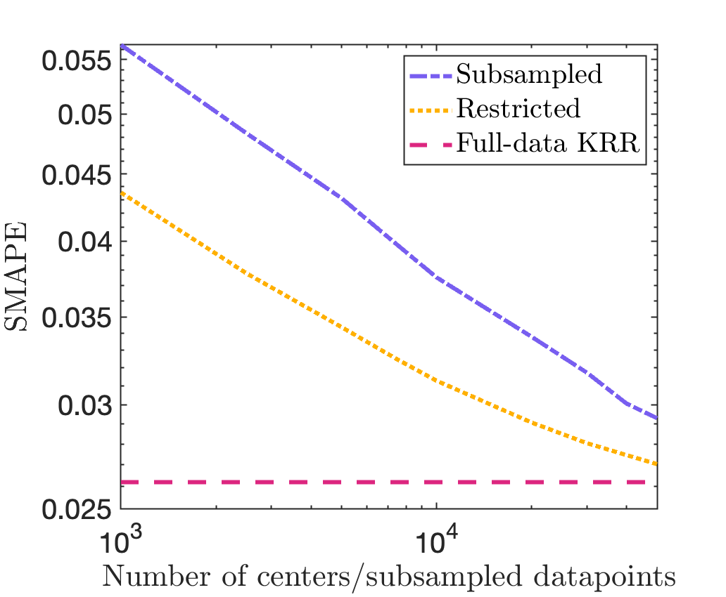
Figure 5: SMAPE versus number of centers / number of subsampled data points for the HOMO energy prediction problem $(N=10^{5})$.

Restricted KRR is a relatively cheap approach for predicting HOMO energies with the QM9 data set, since we can store the $k\times k$ preconditioner and $N\times k$ kernel submatrix in working memory with up to $k=50,000$ centers. Figure 5 shows that restricted KRR is more accurate than randomly subsampling the data and applying full-data KRR to the random sample. Still, the predictive accuracy increases with the number of centers $k$ and does not saturate even when $k=N/2$.

Full-data KRR is the most accurate approach for predicting HOMO energies, but it relies on repeated matrix–vector multiplication with the full kernel matrix. Since the kernel matrix is too large to store in 64GB of working memory, we can only store one block of the matrix at a time and perform the multiplications in a block-wise fashion, with each multiplication requiring tens of minutes of computing. The training of the full-data KRR model is very slow unless we find a preconditioner that controls the total number of CG iterations.

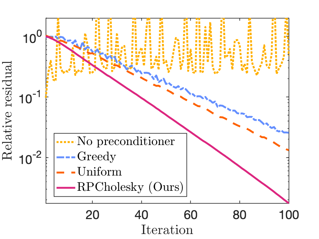
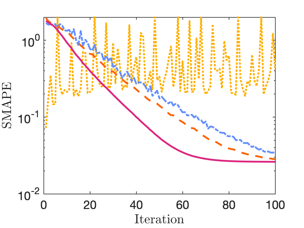
Figure 6: (left) Relative residual $\left\|(\bm{A}+\mu\mathbf{I})\bm{\beta}-\bm{y}\right\|/\left\|\bm{y}\right\|$ and (right) SMAPE for different column Nyström preconditioners.

Figure 6 compares several preconditioning strategies for full-data KRR. The worst strategy is unpreconditioned CG, which leads to no perceivable convergence over the first $100$ iterations. Uniform and greedy Nyström preconditioning (with approximation rank $r=10^{3}$) improve the convergence speed, but they still require $100$ or more iterations for the predictive accuracy to saturate. RPCholesky (also with $r=10^{3}$) is the fastest method, leading to the convergence of the predictive accuracy after $60$ iterations.

Figure 7: Number of CG iterations to achieve a relative residual of $\varepsilon<10^{-3}$ with RPCholesky preconditioning.

Figure 7 shows that we can reduce the total number of CG iterations even further, by a factor of $5\times$, if we increase the RPCholesky approximation rank from $r=10^{3}$ to $r=10^{4}$. However, we also need to consider the cost of preparing the preconditioner, which requires $\mathcal{O}(Nr^{2})$ operations. To achieve an appropriate balance, we recommend tuning the value of $r$ based on computational constraints, and $r$ should typically be small enough that the preconditioner can be stored in working memory. For example, an intermediate value of $10^{3}<r<10^{4}$ would be most appropriate for the HOMO energy prediction problem given our computing architecture.

4.2 Exotic particle detection

The Large Hadron Collider (LHC) is a particle accelerator that is being used to search for exotic particles not included in the standard model of physics. Each second, the LHC collides roughly one billion proton–proton pairs and produces one petabyte of data. Yet, exotic particles are believed to be produced in fewer than one per billion collisions, so only a small fraction of the data is relevant and the LHC is increasingly relying on machine learning to identify the most relevant observations for testing exotic particle models [28].

To help train machine learning algorithms, Baldi, Sadowsky, and Whiteson [6] have produced the SUSY data set ($N=5\times 10^{6}$) from Monte Carlo simulations of the decay processes of standard model bosons and supersymmetric particles not included in the standard model. Following [32, 33, 22], we will apply restricted KRR to the SUSY data to distinguish between the bosonic and supersymmetric decay processes.

For our KRR application, we split the data into $N=4.5\times 10^{6}$ training data points and $M=5\times 10^{5}$ testing data points, and we select $k=10^{4}$ data centers uniformly at random. Then we standardize the data features and apply a squared exponential kernel (2.3) with bandwidth $\sigma=4$. The parameters $k$ and $\sigma$ are the same ones used in previous work [32, 33], but we use a smaller regularization $\mu/N=2\times 10^{-10}$ (compared to $\mu/N=10^{-6}$ in [32, 33, 22]) which improves the test error from $19.6\%$ to $19.5\%$. We apply KRILL, FALKON, and unpreconditioned CG to solve the restricted KRR equations with these parameter choices. We terminate after forty iterations or when the relative residual falls below $\varepsilon=10^{-4}$, leading to the results in Figures 8 and 9.

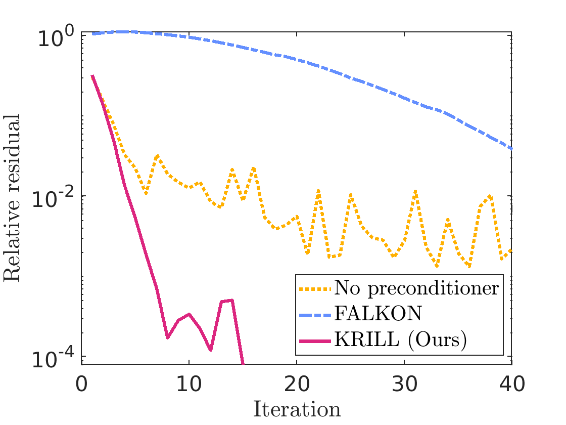
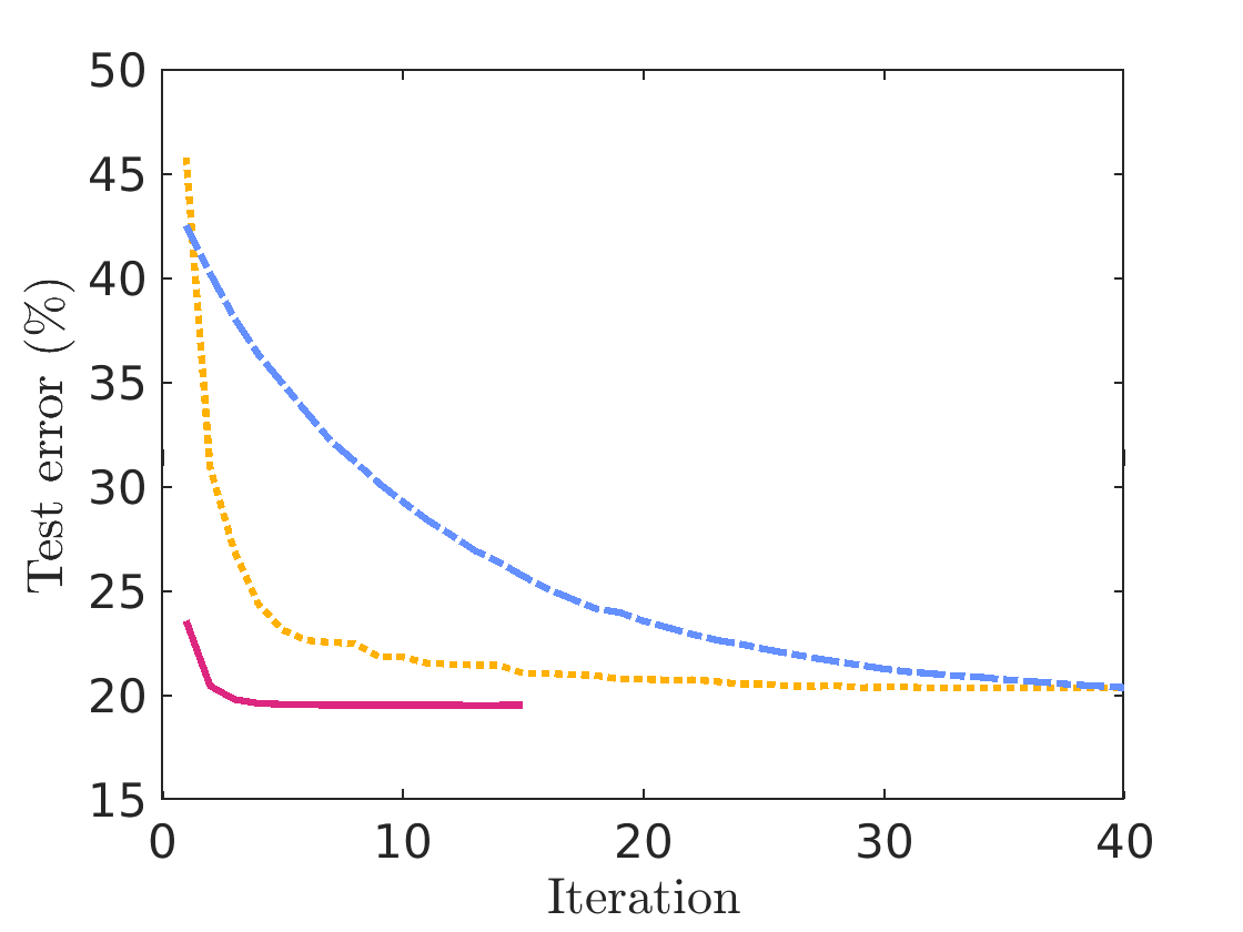
Figure 8: (left) Relative residual $\left\|\smash{(\bm{A}(\mathsf{S},:)\bm{A}(:,\mathsf{S})+\mu\,\bm{A}(\mathsf{S},\mathsf{S}))\,\bm{\widehat{\beta}}-\bm{A}(\mathsf{S},:)\bm{y}}\right\|/\left\|\bm{A}(\mathsf{S},:)\bm{y}\right\|$ and (right) test error for FALKON vs. KRILL.

Figure 8 demonstrates the superior performance of KRILL. KRILL reaches a test error of $19.5\%$ after just four iterations. Meanwhile, unpreconditioned CG fails to achieve such a low test error even after forty iterations, and FALKON converges more slowly than unpreconditioned CG. One reason for the slow convergence of FALKON is the small regularization parameter $\mu/N=2\times 10^{-10}$, which is a known failure mode for the preconditioner [22, Sec. 3]. Indeed, a previous application [33] of FALKON to the SUSY data set with a larger regularization $\mu/N=10^{-6}$ achieved test error convergence more quickly, in just twenty iterations (still five times slower than KRILL). A major advantage of KRILL is the reliable performance for the full range of $\mu$ values, which empowers users to choose the regularization that gives the lowest test error.

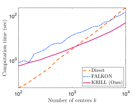
Figure 9: Runtime versus number of centers for the SUSY classification problem ($N=5\times 10^{5}$).

Last, Figure 9 evaluates the total computation time needed to form the preconditioner and solve the restricted KRR equations up to a relative residual of $\varepsilon=10^{-4}$. For this figure, we randomly subsample $N=5\times 10^{5}$ data points so that the kernel submatrix fits in 64GB of working memory, and we compare KRILL, FALKON, and the direct method of forming and inverting $\bm{A}(\mathsf{S},:)\bm{A}(:,\mathsf{S})+\mu\bm{A}(\mathsf{S},\mathsf{S})$. We find that KRILL is the dominant algorithm once the number of centers reaches $k=1250$. KRILL outperforms the direct method because of the superior $\mathcal{O}((N+k^{2})k)$ computational cost, and KRILL outperforms FALKON because it converges in roughly $4\times$ fewer CG iterations.

5 Theoretical results

In this section, we prove our main theoretical results, Theorems 2.2 and 2.3.

5.1 Proof of Theorem 2.2

Let $\bm{\widehat{A}}$ be a Nystrom approximation of the psd matrix $\bm{A}$, and set $\bm{P}=\bm{\widehat{A}}+\mu\mathbf{I}$. As the first step of our proof, we will show that

$$\kappa\bigl{(}\bm{P}^{-1/2}\bigl{(}\bm{A}+\mu\mathbf{I}\bigr{)}\bm{P}^{-1/2}\bigr{)}\leq 1+\operatorname{tr}\bigl{(}\bm{A}-\bm{\widehat{A}}\bigr{)}/\mu.$$ (5.1)

To that end, observe that $\bm{P}\preceq\bm{A}+\mu\mathbf{I}$, because the Nyström approximation $\bm{\widehat{A}}$ is bounded from above by $\bm{A}$. By conjugation with $\bm{P}^{-1/2}$, we obtain

$$\mathbf{I}\preceq\bm{P}^{-1/2}(\bm{A}+\mu\mathbf{I})\bm{P}^{-1/2}$$

and thus

$$1\leq\lambda_{\rm min}\bigl{(}\bm{P}^{-1/2}(\bm{A}+\mu\mathbf{I})\bm{P}^{-1/2}\bigr{)}.$$ (5.2)

Next, a short calculation shows that

$$\bm{P}^{-1/2}(\bm{A}+\mu\mathbf{I})\bm{P}^{-1/2}=\mathbf{I}+\bm{P}^{-1/2}\big{(}\bm{A}-\bm{\widehat{A}}\big{)}\bm{P}^{-1/2}.$$

Since the spectral norm is submultiplicative and equals the largest eigenvalue of a psd matrix, we deduce that

$$\lambda_{\rm max}\bigl{(}\bm{P}^{-1/2}(\bm{A}+\mu\mathbf{I})\bm{P}^{-1/2}\bigr{)} =1+\lambda_{\rm max}\bigl{(}\bm{P}^{-1/2}\big{(}\bm{A}-\bm{\widehat{A}}\big{)}\bm{P}^{-1/2}\bigr{)}$$

$$\leq 1+\left\|\smash{\bm{P}^{-1/2}}\right\|^{2}\left\|\smash{\bm{A}-\bm{\widehat{A}}}\right\|=1+\left\|\smash{\bm{P}^{-1}}\right\|\left\|\smash{\bm{A}-\bm{\widehat{A}}}\right\|.$$

Last, using the fact that $\lVert\bm{A}-\bm{\widehat{A}}\rVert\leq\operatorname{tr}\big{(}\bm{A}-\bm{\widehat{A}}\big{)}$ and $\lambda_{\rm min}(\bm{P})\geq\mu$, we find

$$\lambda_{\rm max}\bigl{(}\bm{P}^{-1/2}(\bm{A}+\mu\mathbf{I})\bm{P}^{-1/2}\bigr{)}\leq 1+\operatorname{tr}\big{(}\bm{A}-\bm{\widehat{A}}\big{)}/\mu.$$ (5.3)

Combining the bound (5.2) for the minimum eigenvalue with the bound (5.3) for the maximum eigenvalue verifies the condition number bound (5.1).

As our next step, we apply the main RPCholesky error bound [10, Thm. 3.1] with rank $r=\text{rank}_{\mu}(\bm{A})$ and approximation accuracy $1+\varepsilon=2$, which guarantees

$$\mathbb{E}\operatorname{tr}\bigl{(}\bm{A}-\bm{\widehat{A}}\bigr{)}\leq 2\sum\nolimits_{i>\text{rank}_{\mu}(\bm{A})}\lambda_{i}(\bm{A})$$ (5.4)

for any $r$ satisfying

$$r\geq\textup{rank}_{\mu}(\bm{A})\,\bigl{(}1+\log\bigl{(}\operatorname{tr}\bm{A}/\mu\bigr{)}\bigr{)}.$$

The right-hand side of (5.4) is bounded by $2\mu$ because of Definition 2.1 of the $\mu$-tail rank of $\bm{A}$. Hence, combining (5.4) with the condition number bound (5.1) guarantees

$$\operatorname{\mathbb{E}}\kappa\Bigl{(}\bm{P}^{-1/2}\big{(}\bm{A}+\mu\mathbf{I}\big{)}\bm{P}^{-1/2}\Bigr{)}\leq 3.$$

By Markov’s inequality, it follows that

$$\kappa\Bigl{(}\bm{P}^{-1/2}\big{(}\bm{A}+\mu\mathbf{I}\big{)}\bm{P}^{-1/2}\Bigr{)}\leq 3/\delta$$

with failure probability at most $\delta$. We apply the CG error bound (3.2) to obtain

$$\frac{\lVert\bm{\beta}^{(t)}-\bm{\beta}\rVert_{\ast}}{\lVert\bm{\beta}\rVert_{\ast}}\leq 2\Biggl{(}\frac{\sqrt{3/\delta}-1}{\sqrt{3/\delta}+1}\Biggr{)}^{t}\leq 2\mathrm{e}^{-2t\sqrt{\delta/3}}\leq 2\mathrm{e}^{-t\sqrt{\delta}}$$

for each $t\geq 0$, with failure probability at most $\delta$, which is equivalent to the stated convergence guarantee for RPCholesky preconditioning.      

5.2 Proof of Theorem 2.3

Cohen [12, Thm. 4.2] showed that a sparse sign embedding with parameters $d=\mathcal{O}(k\log(k/\delta))$ and $\zeta=\mathcal{O}(\log(k/\delta))$ satisfies the following oblivious subspace embedding property: for any $k$-dimensional subspace $\mathsf{X}\subseteq{}^{N}$, there is probability at least $1-\delta$ that

$$(1/2)\left\|\bm{v}\right\|^{2}\leq\left\|\bm{\Phi}\bm{v}\right\|^{2}\leq(3/2)\left\|\bm{v}\right\|^{2}\quad\text{for every $\bm{v}\in\mathsf{X}$}.$$ (5.5)

We set $\mathsf{X}=\textup{range}(\bm{A}(:,\mathsf{S}))$ and consider the matrices

$$\bm{P}=\bm{A}(\mathsf{S},:)\bm{\Phi}^{\ast}\bm{\Phi}\bm{A}(:,\mathsf{S})+\mu\,\bm{A}(\mathsf{S},\mathsf{S})\quad\text{and}\quad\bm{M}=\bm{A}(\mathsf{S},:)\bm{A}(:,\mathsf{S})+\mu\,\bm{A}(\mathsf{S},\mathsf{S}).$$

By the subspace embedding property (5.5),

$$\lambda_{\rm max}\left(\bm{P}^{-1/2}\bm{M}\bm{P}^{-1/2}\right) =\max_{\bm{z}\neq\bm{0}}\frac{\bm{z}^{*}\bm{M}\bm{z}}{\bm{z}^{*}\bm{P}\bm{z}}\leq\max_{\bm{z}\neq\bm{0}}\;\max\Biggl{\{}1,\frac{\left\|\bm{A}(:,\mathsf{S})\bm{z}\right\|^{2}}{\left\|\bm{\Phi}\bm{A}(:,\mathsf{S})\bm{z}\right\|^{2}}\Biggr{\}}\leq 2;$$

$$\lambda_{\rm min}\left(\bm{P}^{-1/2}\bm{M}\bm{P}^{-1/2}\right) =\min_{\bm{z}\neq\bm{0}}\frac{\bm{z}^{*}\bm{M}\bm{z}}{\bm{z}^{*}\bm{P}\bm{z}}\geq\min_{\bm{z}\neq\bm{0}}\;\min\Biggl{\{}1,\frac{\left\|\bm{A}(:,\mathsf{S})\bm{z}\right\|^{2}}{\left\|\bm{\Phi}\bm{A}(:,\mathsf{S})\bm{z}\right\|^{2}}\Biggr{\}}\geq\frac{2}{3}.$$

Therefore, $\kappa(\bm{P}^{-1/2}\bm{M}\bm{P}^{-1/2})\leq 3$, and we apply the CG error bound (3.2) to obtain

$$\frac{\lVert\bm{\beta}^{(t)}-\bm{\beta}\rVert_{\ast}}{\lVert\bm{\beta}\rVert_{\ast}}\leq 2\Biggl{(}\frac{\sqrt{3}-1}{\sqrt{3}+1}\Biggr{)}^{t}\leq 2\mathrm{e}^{-t}$$

for each $t\geq 0$, which is equivalent to the stated performance guarantee.      

6 Conclusions

We have presented two new algorithms for solving kernel ridge regression (KRR) problems with a moderate or large number of data points ($10^{4}\leq N\leq 10^{7}$). Our proposed algorithms based on RPCholesky and KRILL preconditioning are fast, robust, and reliable, outperforming previous approaches [13, 18, 19, 40, 32, 33, 25].

If the number of data points $N$ is not prohibitively large (say, $N\leq 10^{5}$–$10^{6}$), we recommend solving the full-data KRR equations using conjugate gradient with RPCholesky preconditioning. As long as the kernel matrix eigenvalues have polynomial or faster decay, the RPCholesky approach enables us solve KRR problems in just $\mathcal{O}(N^{2})$ operations. In our application to the QM9 data set ($N=1.3\times 10^{5}$ data points), we only require $60$ CG iterations to acheive a high predictive accuracy using RPCholesky, and CG converges even faster when we use RPCholesky with a higher approximation rank.

If the number of data points is so large that $\mathcal{O}(N^{2})$ operations is too expensive, we recommend restricting the KRR equations to $k\ll N$ data centers and solving the restricted KRR equations using conjugate gradient with KRILL preconditioning. The KRILL approach converges to the desired accuracy in just $\mathcal{O}((N+k^{2})k\log k)$ operations, for any kernel matrix and regularization parameter $\mu$. In our application to the SUSY data set ($N=5\times 10^{6}$ data points), KRILL converges in just $4$ iterations, even with a parameter setting $\mu/N=2\times 10^{-10}$ that would be challenging for other algorithms. Just as krill are the foundation for the marine ecosystem, the KRILL algorithm has the potential to serve as the foundation for many large-scale KRR applications in the future.

Appendix A Data sets

In our numerical experiments, we use data from LIBSVM [8], OpenML [39], and UCI [17]. We also use the QM9 dataset [29, 31] which can be found online at https://doi.org/10.6084/m9.figshare.c.978904.v5. See the Github repository https://github.com/eepperly/Fast-Efficient-KRR-Preconditioning for a script to download the data sets.

Table 1: Data sets used in our experiments.

Data set	Dimension $d$	Sample size $N$	Source
Testbed
ACSIncome	11	1 331 600	OpenML
Airlines_DepDelay_1M	9	800 000	OpenML
cod_rna	8	59 535	LIBSVM
COMET_MC_SAMPLE	4	71 712	LIBSVM
connect_4	126	54 045	LIBSVM
covtype_binary	54	464 809	LIBSVM
creditcard	29	227 845	OpenML
diamonds	9	43 152	OpenML
HIGGS	28	500 000	LIBSVM
hls4ml_lhc_jets_hlf	16	664 000	OpenML
ijcnn1	22	49 990	LIBSVM
jannis	54	46 064	OpenML
Medical_Appointment	18	48 971	OpenML
MNIST	784	60 000	OpenML
santander	200	160 000	OpenML
sensit_vehicle	100	78 823	LIBSVM
sensorless	48	58 509	LIBSVM
volkert	180	46 648	OpenML
w8a	300	49 749	LIBSVM
YearPredictionMSD	90	463 715	LIBSVM
yolanda	100	320 000	OpenML
Additional data sets
QM9	435	133 728	[29, 31]
SUSY	18	5 000 000	UCI

References

- Alaoui and Mahoney [2015] A. Alaoui and M. W. Mahoney. Fast randomized kernel ridge regression with statistical guarantees. In Advances in Neural Information Processing Systems, volume 28, 2015.
- Ambikasaran et al. [2016] S. Ambikasaran, D. Foreman-Mackey, L. Greengard, D. W. Hogg, and M. O’Neil. Fast Direct Methods for Gaussian Processes. IEEE Transactions on Pattern Analysis and Machine Intelligence, 38(2):252–265, 2016. doi:10.1109/TPAMI.2015.2448083.
- Avron et al. [2010] H. Avron, P. Maymounkov, and S. Toledo. Blendenpik: Supercharging LAPACK’s Least-Squares Solver. SIAM Journal on Scientific Computing, 32(3):1217–1236, 2010. doi:10.1137/090767911.
- Avron et al. [2017] H. Avron, K. L. Clarkson, and D. P. Woodruff. Faster kernel ridge regression using sketching and preconditioning. SIAM Journal on Matrix Analysis and Applications, 38(4):1116–1138, 2017. doi:10.1137/16M1105396.
- Bach [2013] F. Bach. Sharp analysis of low-rank kernel matrix approximations. In Proceedings of the 26th Annual Conference on Learning Theory, volume 30 of Proceedings of Machine Learning Research, pages 185–209, 2013. URL https://proceedings.mlr.press/v30/Bach13.html.
- Baldi et al. [2014] P. Baldi, P. Sadowski, and D. Whiteson. Searching for exotic particles in high-energy physics with deep learning. Nature Communications, 5(1):1–9, 2014. doi:10.1038/ncomms5308.
- Blücher et al. [2022] S. Blücher, K.-R. Müller, and S. Chmiela. Reconstructing kernel-based machine learning force fields with super-linear convergence. arXiv:2212.12737, 2022. URL https://arxiv.org/abs/2212.12737.
- Chang and Lin [2011] C.-C. Chang and C.-J. Lin. LIBSVM: A library for support vector machines. ACM Transactions on Intelligent Systems and Technology, 2(3), 2011. doi:10.1145/1961189.1961199.
- Chen et al. [2017] J. Chen, H. Avron, and V. Sindhwani. Hierarchically compositional kernels for scalable nonparametric learning. Journal of Machine Learning Research, 18(66):1–42, 2017. URL http://jmlr.org/papers/v18/15-376.html.
- Chen et al. [2022] Y. Chen, E. N. Epperly, J. A. Tropp, and R. J. Webber. Randomly pivoted Cholesky: Practical approximation of a kernel matrix with few entry evaluations. arXiv:2207.06503, 2022. URL https://arxiv.org/abs/2207.06503.
- Clarkson and Woodruff [2017] K. L. Clarkson and D. P. Woodruff. Low-rank approximation and regression in input sparsity time. Journal of the ACM, 63(6), 2017. doi:10.1145/3019134.
- Cohen [2016] M. B. Cohen. Nearly tight oblivious subspace embeddings by trace inequalities. In Proceedings of the 2016 Annual ACM-SIAM Symposium on Discrete Algorithms, pages 278–287, 2016. doi:10.1137/1.9781611974331.ch21.
- Cutajar et al. [2016] K. Cutajar, M. Osborne, J. Cunningham, and M. Filippone. Preconditioning kernel matrices. In Proceedings of The 33rd International Conference on Machine Learning, volume 48 of Proceedings of Machine Learning Research, pages 2529–2538, 2016. URL https://proceedings.mlr.press/v48/cutajar16.html.
- Dai et al. [2014] B. Dai, B. Xie, N. He, Y. Liang, A. Raj, M.-F. F. Balcan, and L. Song. Scalable kernel methods via doubly stochastic gradients. In Advances in Neural Information Processing Systems, volume 27, 2014.
- Deringer et al. [2021] V. L. Deringer, A. P. Bartók, N. Bernstein, D. M. Wilkins, M. Ceriotti, and G. Csányi. Gaussian process regression for materials and molecules. Chemical Reviews, 121(16):10073–10141, 2021. doi:10.1021/acs.chemrev.1c00022.
- Dong and Martinsson [2021] Y. Dong and P.-G. Martinsson. Simpler is better: A comparative study of randomized algorithms for computing the CUR decomposition. arXiv:2104.05877, 2021. URL https://arxiv.org/abs/2104.05877.
- Dua and Graff [2017] D. Dua and C. Graff. UCI machine learning repository, 2017. URL http://archive.ics.uci.edu/ml.
- Frangella et al. [2021] Z. Frangella, J. A. Tropp, and M. Udell. Randomized Nyström Preconditioning. arXiv:2110.02820, 2021. URL https://arxiv.org/abs/2110.02820.
- Gardner et al. [2018] J. Gardner, G. Pleiss, K. Q. Weinberger, D. Bindel, and A. G. Wilson. GPyTorch: Blackbox matrix-matrix Gaussian process inference with GPU acceleration. In Advances in Neural Information Processing Systems, volume 31, 2018.
- Golub and Van Loan [2013] G. H. Golub and C. F. Van Loan. Matrix Computations. Johns Hopkins University Press, 2013. doi:10.56021/9781421407944.
- Lacotte and Pilanci [2021] J. Lacotte and M. Pilanci. Fast convex quadratic optimization solvers with adaptive sketching-based preconditioners. arXiv:2104.14101, 2021. URL https://arxiv.org/abs/2104.14101.
- Letizia et al. [2022] M. Letizia, G. Losapio, M. Rando, G. Grosso, A. Wulzer, M. Pierini, M. Zanetti, and L. Rosasco. Learning new physics efficiently with nonparametric methods. The European Physical Journal C, 82(10):879, 2022. doi:10.1140/epjc/s10052-022-10830-y.
- Ma and Belkin [2017] S. Ma and M. Belkin. Diving into the shallows: A computational perspective on large-scale shallow learning. In Advances in Neural Information Processing Systems, volume 30, 2017.
- Martinsson and Tropp [2020] P.-G. Martinsson and J. A. Tropp. Randomized numerical linear algebra: Foundations and algorithms. Acta Numerica, 29:403–572, 2020. doi:10.1017/S0962492920000021.
- Meanti et al. [2020] G. Meanti, L. Carratino, L. Rosasco, and A. Rudi. Kernel methods through the roof: Handling billions of points efficiently. In Advances in Neural Information Processing Systems, volume 33, 2020.
- Meier and Nakatsukasa [2022] M. Meier and Y. Nakatsukasa. Randomized algorithms for Tikhonov regularization in linear least squares. arXiv:2203.07329, 2022. URL https://arxiv.org/abs/2203.07329.
- Meng et al. [2014] X. Meng, M. A. Saunders, and M. W. Mahoney. LSRN: A parallel iterative solver for strongly over- or underdetermined systems. SIAM Journal on Scientific Computing, 36(2):C95–C118, 2014. doi:10.1137/120866580.
- Radovic et al. [2018] A. Radovic, M. Williams, D. Rousseau, M. Kagan, D. Bonacorsi, A. Himmel, A. Aurisano, K. Terao, and T. Wongjirad. Machine learning at the energy and intensity frontiers of particle physics. Nature, 560(7716):41–48, 2018. doi:10.1038/s41586-018-0361-2.
- Ramakrishnan et al. [2014] R. Ramakrishnan, P. O. Dral, M. Rupp, and O. A. von Lilienfeld. Quantum chemistry structures and properties of 134 kilo molecules. Scientific Data, 1(1):140022, 2014. ISSN 2052-4463. doi:10.1038/sdata.2014.22.
- Rokhlin and Tygert [2008] V. Rokhlin and M. Tygert. A fast randomized algorithm for overdetermined linear least-squares regression. Proceedings of the National Academy of Sciences, 105(36):13212–13217, 2008. doi:10.1073/pnas.0804869105.
- Ruddigkeit et al. [2012] L. Ruddigkeit, R. van Deursen, L. C. Blum, and J.-L. Reymond. Enumeration of 166 billion organic small molecules in the chemical universe database GDB-17. Journal of Chemical Information and Modeling, 52(11):2864–2875, 2012. doi:10.1021/ci300415d.
- Rudi et al. [2017] A. Rudi, L. Carratino, and L. Rosasco. FALKON: An optimal large scale kernel method. In Advances in Neural Information Processing Systems, volume 30, 2017.
- Rudi et al. [2018] A. Rudi, D. Calandriello, L. Carratino, and L. Rosasco. On fast leverage score sampling and optimal learning. In Advances in Neural Information Processing Systems, volume 31, 2018.
- Saad [2003] Y. Saad. Iterative Methods for Sparse Linear Systems. Society for Industrial and Applied Mathematics, second edition, 2003. doi:10.1137/1.9780898718003.
- Smola and Bartlett [2000] A. Smola and P. Bartlett. Sparse greedy Gaussian process regression. In Advances in Neural Information Processing Systems, volume 13, 2000.
- Stuke et al. [2019] A. Stuke, M. Todorović, M. Rupp, C. Kunkel, K. Ghosh, L. Himanen, and P. Rinke. Chemical diversity in molecular orbital energy predictions with kernel ridge regression. The Journal of Chemical Physics, 150(20):204121, 2019. doi:10.1063/1.5086105.
- Tropp et al. [2019] J. A. Tropp, A. Yurtsever, M. Udell, and V. Cevher. Streaming low-rank matrix approximation with an application to scientific simulation. SIAM Journal on Scientific Computing, 41(4):A2430–A2463, 2019. doi:10.1137/18M1201068.
- Unke et al. [2021] O. T. Unke, S. Chmiela, H. E. Sauceda, M. Gastegger, I. Poltavsky, K. T. Schütt, A. Tkatchenko, and K.-R. Müller. Machine learning force fields. Chemical Reviews, 121(16):10142–10186, 2021. doi:10.1021/acs.chemrev.0c01111.
- Vanschoren et al. [2013] J. Vanschoren, J. N. van Rijn, B. Bischl, and L. Torgo. OpenML: Networked science in machine learning. ACM Special Interest Group on Knowledge Discovery in Data Explorations Newsletter, 15(2):49–60, 2013. doi:10.1145/2641190.2641198.
- Wang et al. [2019] K. Wang, G. Pleiss, J. Gardner, S. Tyree, K. Q. Weinberger, and A. G. Wilson. Exact Gaussian processes on a million data points. In Advances in Neural Information Processing Systems, volume 32, 2019.
- Westermayr and Marquetand [2021] J. Westermayr and P. Marquetand. Machine learning for electronically excited states of molecules. Chemical Reviews, 121(16):9873–9926, 2021. doi:10.1021/acs.chemrev.0c00749.
- Yang et al. [2012] T. Yang, Y.-f. Li, M. Mahdavi, R. Jin, and Z.-H. Zhou. Nyström method vs random Fourier features: A theoretical and empirical comparison. In Advances in Neural Information Processing Systems, volume 25, 2012.
- Yu et al. [2017] C. D. Yu, J. Levitt, S. Reiz, and G. Biros. Geometry-oblivious FMM for compressing dense SPD matrices. In Proceedings of the International Conference for High Performance Computing, Networking, Storage and Analysis, 2017. doi:10.1145/3126908.3126921.