Exact Bayesian Geostatistics Using Predictive Stacking

Abstract

We develop Bayesian predictive stacking for geostatistical models. Our approach builds an augmented Bayesian linear regression framework that subsumes the realisations of the spatial random field and delivers exact analytically tractable posterior inference conditional upon certain spatial process parameters. We subsequently combine such inference by stacking these individual models across the range of values of the hyper-parameters. We devise stacking of means and posterior densities in a manner that is computationally efficient without the need of iterative algorithms such as Markov chain Monte Carlo (MCMC) and can exploit the benefits of parallel computations. We offer novel theoretical insights into the resulting inference within an infill asymptotic paradigm and through empirical results showing that stacked inference is comparable to full sampling-based Bayesian inference at a significantly lower computational cost.

.

1 Introduction

Geostatistics (Cressie, 1993; Chilés & Delfiner, 1999; Zimmerman & Stein, 2010; Banerjee, 2019) refers to the study of a spatially distributed variable of interest, which in theory is defined at every point over a bounded study region of interest. Customary geostatistical modelling proceeds from a latent stochastic process over space that specifies the probability law for the point-referenced measurements on the variable as a partial realisation of the process over a finite set of locations. Inference is sought for the underlying spatial process posited to be generating the data, which is subsequently used for spatial predictions over the domain (“kriging” Stein, 1999) to better understand the scientific phenomenon under study. The spatial process, is often assumed to be stationary and empirically estimated from measurements at sampled locations using the “variogram” and characterised by parameters representing the sill, the nugget, the range and, possibly, the smoothness of the process. We collectively refer to these as process parameters.

Formal likelihood-based inference for this process is, however, thwarted by the absence of classical consistent estimators of the process parameters in a customarily preferred infill asymptotic paradigm (see, e.g., Stein, 1999; Zhang, 2004; Zhang & Zimmerman, 2005; Kaufman & Shaby, 2013; Tang et al., 2021). Bayesian inference for geostatistical processes (Handcock & Stein, 1993; Berger et al., 2001; Banerjee et al., 2014; Li et al., 2023), while not relying upon asymptotic inference, is also not entirely straightforward. Specifically, irrespective of how many spatial locations yield measurements, the likelihood does not mitigate the effect of the prior distributions on the inference. This is undesirable since proper prior elicitation for spatial process parameters is challenging. Objective priors for spatial process models have also been pursued, but interpreting such information in practice and their implications in scientific contexts are not uncontroversial. The related question of how effectively (or poorly) the realised data can identify these process parameters (in an exact sense from finite samples) has also been the subject of commentary (see, e.g., Hodges, 2013; Bose et al., 2018; De Oliveira & Han, 2022).

The aforementioned, rather substantial, literature has focused extensively on inference for geostatistical parameters and their sensitivity to modelling assumptions from diverse perspectives. It is, therefore, not unreasonable to pursue methods that will yield robust inference for the spatial process and for spatial predictions of the outcome at arbitrary points (“kriging”) while circumventing inference on the weakly identified parameters. Instead of seeking families of prior distributions for such parameters, recent efforts at computationally efficient algorithms for geostatistical models have proposed multi-fold cross-validation methods (Finley et al., 2019) to fix the values of weakly identified parameters. However, the metrics for ascertaining optimal values of such parameters are somewhat arbitrary and may not offer robust inference. Instead, our current contribution develops Bayesian predictive stacking of geostatistical models.

Stacking is a model averaging procedure for generating predictions (Wolpert, 1992; Breiman, 1996a; Clyde & Iversen, 2013). Stacking methods and algorithms in diverse data analytic applications are rapidly evolving and a comprehensive review is beyond the scope of this manuscript. Significant developments of stacking methodology in Bayesian analysis have been achieved in recent years (Le & Clarke, 2017; Yao et al., 2018, 2020, 2021), but, to the best of our knowledge, developments in the context of spatial data analysis are lacking. Stacking can be regarded as an alternative to Bayesian model averaging (Madigan et al., 1996; Hoeting et al., 1999). Assume that there are $G$ candidate models ${\cal M}=\{M_{1},\ldots,M_{G}\}$. Following Bernardo & Smith (1994), Bayesian model comparison customarily considers three settings: (i) ${\cal M}$-closed where a true data generating model exists and is included in ${\cal M}$; (ii) ${\cal M}$-complete where a true model exists but is not included in ${\cal M}$; and (iii) ${\cal M}$-open where we do not assume the existence of a true data generating model. While Bayesian model averaging is often the preferred solution in the first setting, predictive stacking has advantages in the ${\cal M}$-complete and ${\cal M}$-open settings. Given the complex nature of spatial dependence, the ${\cal M}$-closed assumption is rarely tenable in practical geostatistics and we prefer stacking to model averaging.

Much of the theoretical properties of conventional stacking rely upon properties of exchangeable models that are not enjoyed by geostatistical models. Inferential behaviour of posterior distributions is, therefore, studied within an infill asymptotic paradigm. We absorb spatial process realisations into a convenient augmented Bayesian linear regression framework (Section 2). We offer some novel theoretical insights into the consistency of the posterior and posterior predictive distributions. Each model $M_{g}\in{\cal M}$ is indexed according to fixed values of certain spatial covariance parameters so that the exact posterior distribution is analytically tractable. Section 3 develops geostatistical predictive stacking by combining the exact inference across the $G$ models in ${\cal M}$. We develop (i) stacking of means, which combines posterior predictive means, $\mathbb{E}_{g}(\tilde{y}(s_{0})\,|\,y_{obs},M_{g})$, from each of the $G$ models; and (ii) stacking of posterior predictive densities (Yao et al., 2018), which combines posterior predictive densities $p(\tilde{y}(s_{0})\,|\,y_{obs},M_{g})$ for $g=1,2,\ldots,G$, where $\tilde{y}(s_{0})$ is the random variable denoting model predictions of the outcome at an arbitrary point $s_{0}$ and $y_{obs}$ denotes the observed data on the outcome. We obtain exact Bayesian inference by exploiting exact distribution theory and avoiding iterative algorithms such as Markov chain Monte Carlo (MCMC). These methods are evaluated theoretically as well as empirically through simulation experiments (Section 4) demonstrating that stacked inference is comparable to full Bayesian inference using MCMC at significantly less computational expense. An illustrative data analysis is presented in Section 5 to further corroborate results seen in the simulations. We conclude with some discussions and pointers to future work in Section 6.

2 Bayesian hierarchical spatial process models

2.1 Conjugate Bayesian spatial model

We explore a regression model for a spatially indexed outcome $y(s)$ at a location $s$ in a bounded region $\mathcal{D}\subset\mathbb{R}^{d}$,

$$y(s)=x(s)^{\mathrm{\scriptscriptstyle T}}\beta+z(s)+\varepsilon(s),$$ (2.1)

where $x(s)$ is a $p\times 1$ vector of spatially referenced predictors, $\beta$ is a $p\times 1$ vector of slopes measuring the trend, $z(s)\sim\mbox{GP}(0,\sigma^{2}R_{\phi}(\cdot,\cdot))$ is a zero-centred spatial Gaussian process on $\mathbb{R}^{d}$ with spatial correlation function $R_{\phi}(\cdot,\cdot)$ depending on spatial range parameter $\phi$, and $\sigma^{2}$ is a scale (spatial variance) parameter. The white noise process $\varepsilon(s)\sim\mathcal{N}(0,\tau^{2})$ with variance $\tau^{2}$ captures measurement error.

Let $\chi=\{s_{1},\ldots,s_{n}\}$ be a set of $n$ spatial locations, each $s_{i}\in\mathcal{D}$, yielding measurements $y=(y(s_{1}),\ldots,y(s_{n}))^{\mathrm{\scriptscriptstyle T}}$ with known values of predictors at these locations collected in the $n\times p$ matrix $X=(x(s_{1}),\cdots,x(s_{n}))^{\mathrm{\scriptscriptstyle T}}$. We also define the finite-dimensional realisation of the spatial process as $z=(z(s_{1}),\ldots,z(s_{n}))^{\mathrm{\scriptscriptstyle T}}$, and let $R_{\phi}(\chi)=(R_{\phi}(s_{i},s_{j}))_{1\leq i,j\leq n}$ be the $n\times n$ spatial correlation matrix constructed from the correlation function. A customary Bayesian hierarchical model is constructed as

$$y\,| z,\beta,\sigma^{2}\sim\mathcal{N}(X\beta+z,\delta^{2}\sigma^{2}I_{n}),\quad z\,|\,\sigma^{2}\sim\mathcal{N}(0,\sigma^{2}R_{\phi}(\chi))$$ (2.2)

$$\beta\,| \sigma^{2}\sim\mathcal{N}(\mu_{\beta},\sigma^{2}V_{\beta}),\quad\sigma^{2}\sim\mbox{IG}(a_{\sigma},b_{\sigma}),$$

where we fix the spatial correlation parameters $\phi$ and the noise-to-spatial variance ratio $\delta^{2}:=\frac{\tau^{2}}{\sigma^{2}}$, and $\mu_{\beta}$, $V_{\beta}$, $a_{\sigma}$, and $b_{\sigma}$ are fixed hyper-parameters specifying the prior distributions for $\beta$ and $\sigma^{2}$. This ensures closed-form conjugate marginal posterior and posterior predictive distributions (Finley et al., 2019; Banerjee, 2020). In order to harness familiar results from conjugate Bayesian linear regression, we cast the spatial model in (2.2) into an augmented linear system:

$$\underbrace{\begin{pmatrix}y\\ \mu_{\beta}\\ 0\end{pmatrix}}_{y_{*}}=\underbrace{\begin{pmatrix}X&I_{n}\\ I_{p}&0\\ 0&I_{n}\end{pmatrix}}_{X_{*}}\underbrace{\begin{pmatrix}\beta\\ z\end{pmatrix}}_{\gamma}+\underbrace{\begin{pmatrix}\eta_{1}\\ \eta_{2}\\ \eta_{3}\end{pmatrix}}_{\eta},$$ (2.3)

where $\eta\sim\mathcal{N}(0,\sigma^{2}V_{y_{*}})$, $\displaystyle V_{*}=\begin{pmatrix}\delta^{2}I_{n}&0&0\\ 0&V_{\beta}&0\\ 0&0&R_{\phi}(\chi)\end{pmatrix}$ and $p(\gamma,\sigma^{2})\propto\mbox{IG}(\sigma\,|\,a_{\sigma},b_{\sigma})$.

Lemma 2.1.

The posterior distribution of $(\gamma,\sigma^{2})$ from (2.2) is

$$p(\gamma,\sigma^{2}\,|\,y)=\underbrace{\mbox{IG}(\sigma^{2}\,|\,a^{*}_{\sigma},b^{*}_{\sigma})}_{p(\sigma^{2}\,|\,y)}\times\underbrace{\mathcal{N}(\gamma\,|\,\hat{\gamma},\sigma^{2}M_{*})}_{p(\gamma\,|\,\sigma^{2},y)},$$ (2.4)

where $a^{*}_{\sigma}=a_{\sigma}+n/2$, $b^{*}_{\sigma}=b_{\sigma}+\frac{1}{2}(y_{*}-X_{*}\hat{\gamma})^{{\mathrm{\scriptscriptstyle T}}}V_{*}^{-1}(y_{*}-X_{*}\hat{\gamma})$, $M_{*}^{-1}=X_{*}^{\mathrm{\scriptscriptstyle T}}V_{*}^{-1}X_{*}$ and $\hat{\gamma}=M_{\ast}X_{*}^{{\mathrm{\scriptscriptstyle T}}}V_{*}^{-1}y_{*}$. The posterior distribution $p(\gamma\,|\,y)$ is a multivariate Student’s t with degrees of freedom $2a_{\sigma}^{\ast}$, location $\hat{\gamma}$ and scale matrix $(b_{\sigma}^{\ast}/a_{\sigma}^{\ast})M_{\ast}$.

Proof 2.2.

The proof follows from a straightforward adaptation of familiar results from the Normal-Gamma family of distributions (see (Murphy, 2015) and Section 3.1 in (Banerjee, 2020)) to the setting in (2.3).

Furthermore, let $\tilde{\chi}=\{\tilde{s}_{1},\ldots,\tilde{s}_{m}\}$ be a set of $m$ unknown points in ${\cal D}$, $\tilde{z}$ and $\tilde{y}$ be the $m\times 1$ vectors with elements $z(\tilde{s}_{i})$ and $y(\tilde{s}_{i})$ for $i=1,2,\ldots,m$. Let $\tilde{X}=(x(\tilde{s}_{1}),\ldots,x(\tilde{s}_{m}))^{\mathrm{\scriptscriptstyle T}}$ be the $m\times p$ matrix that carries the values of predictors at $\tilde{\chi}$ and let $J_{\phi}(\tilde{\chi})=(R_{\phi}(s,s^{\prime}))_{\{s\in\chi,s^{\prime}\in\tilde{\chi}\}}$ Then, spatial predictive inference follows from the posterior distribution

$$p(\tilde{z},\tilde{y}\,|\,y)=\int p(\tilde{y}\,|\,\tilde{z},\beta,\sigma^{2})p(\tilde{z}\,|\,z,\sigma^{2})p(\gamma,\sigma^{2}\,|\,y)\mathop{d\gamma}\mathop{d\sigma^{2}}\;,$$ (2.5)

which is again a multivariate $t$ distribution with degrees of freedom $2a_{\sigma}^{\ast}$, location $\tilde{\mu}$ and scale matrix $(b_{\sigma}^{\ast}/a_{\sigma}^{\ast})\tilde{M}$ where

$$\tilde{\mu}=W\hat{\gamma}\;,\;\tilde{M}=WM_{\ast}W^{\mathrm{\scriptscriptstyle T}}+M_{2}\; ,\;M_{1}=I_{m}-J_{\phi}^{\mathrm{\scriptscriptstyle T}}(\tilde{\chi})R_{\phi}^{-1}(\chi)J_{\phi}(\tilde{\chi})\;,\;$$

$$W=\begin{bmatrix}0&-J_{\phi}^{\mathrm{\scriptscriptstyle T}}(\tilde{\chi})R_{\phi}^{-1}(\chi)\\ \tilde{X}&-J_{\phi}^{\mathrm{\scriptscriptstyle T}}(\tilde{\chi})R_{\phi}^{-1}(\chi)\end{bmatrix}\; ,\;M_{2}^{-1}=\begin{bmatrix}\frac{1}{\delta^{2}}I_{m}+M_{1}^{-1}&-\frac{1}{\delta^{2}}I_{m}\\ -\frac{1}{\delta^{2}}I_{m}&\frac{1}{\delta^{2}}I_{m}\end{bmatrix}\;.$$

Specifically, the predictive distributions $p(z(s_{0})\,|\,y)$ and $p(y(s_{0})\,|\,y)$ are also available in analytic form as non-central t distributions for any single point $s_{0}\in{\cal D}$. Bayesian inference can proceed from exact posterior samples obtained from (2.4) as follows. We first draw values of $\sigma^{2}\sim IG(a_{\sigma}^{\ast},b_{\sigma}^{\ast})$ followed by a single draw of $\gamma\sim N(\hat{\gamma},\sigma^{2}M_{\ast})$ for each drawn value of $\sigma^{2}$. This yields samples $\{\gamma,\sigma^{2}\}$ from (2.4). Predictive inference for the latent process $z(s_{0})$ and the outcome $y(s_{0})$ is obtained by sampling from (2.5) by drawing a value of $\tilde{z}\sim N(\mu_{z}(\gamma),\sigma^{2}V_{z|\cdot})$ with $\mu_{z}(\gamma):=J_{\phi}^{\mathrm{\scriptscriptstyle T}}(\tilde{\chi})R_{\phi}(\chi)^{-1}z$ and $V_{z|\cdot}:=R_{\phi}(\tilde{\chi})-J_{\phi}^{\mathrm{\scriptscriptstyle T}}(\tilde{\chi})R_{\phi}(\chi)^{-1}J_{\phi}(\tilde{\chi})$ for each value of $\{\gamma,\sigma^{2}\}$ drawn above (see Section 3.4 in Banerjee (2020)), then drawing a value of $\tilde{y}\sim N(\tilde{X}\beta+\tilde{z},\sigma^{2}\delta^{2}I_{m})$ for each drawn value of $\beta$ (extracted from $\gamma$), $\sigma^{2}$ and $\tilde{z}$.

This tractability is only possible if the range decay $\phi$ and the noise-to-spatial variance ratio $\delta^{2}$ are fixed. While the data can inform about these parameters, they are inconsistently estimable (Zhang, 2004) often resulting in poorer convergence. Alternate approaches using $K$-fold cross-validation have been explored with limited success (Finley et al., 2019). Therefore, our approach will conduct the exact inference using (2.4) and (2.5) and stack the inference over the different fixed values of $\{\phi,\delta^{2}\}$. Next, we investigate the concentration of the posteriors and the effect of incorrectly specified hyperparameters on the posterior inference.

2.2 Posterior inference for spatial process models

Let $L_{\beta}$ be the Cholesky decomposition of $V_{\beta}$ such that $V_{\beta}=L_{\beta}L_{\beta}^{\mathrm{\scriptscriptstyle T}}$, and $L_{\phi}$ a non-singular square matrix such that $R_{\phi}(\chi)^{-1}=L_{\phi}^{\mathrm{\scriptscriptstyle T}}L_{\phi}$. The linear model (2.3) can be rewritten as

$$\underbrace{\begin{pmatrix}\frac{1}{\delta}y\\ L_{\beta}^{-1}\mu_{\beta}\\ 0\end{pmatrix}}_{y_{\dagger}}=\underbrace{\begin{pmatrix}\frac{1}{\delta}X&\frac{1}{\delta}I_{n}\\ L_{\beta}^{-1}&0\\ 0&L_{\phi}\end{pmatrix}}_{X_{\dagger}}\underbrace{\begin{pmatrix}\beta\\ z\end{pmatrix}}_{\gamma}+\underbrace{\begin{pmatrix}\eta_{\dagger,1}\\ \eta_{\dagger,2}\\ \eta_{\dagger,3}\end{pmatrix}}_{\eta_{\dagger}},$$ (2.6)

where $\eta_{\dagger}\sim\mathcal{N}(0,\sigma^{2}I_{2n+p})$. To explore posterior concentrations within an in-fill paradigm, where we assume a fixed size of our spatial domain ${\cal D}$ and an increasing number of spatial locations inside ${\cal D}$, we will use the concept of equivalence of probability measures.

[Equivalence] Let $\mathbb{P}_{0}$ be the probability distribution of the process $y(s)$ defined by the model (2.1) with true parameter values $\{\beta_{0},\sigma_{0}^{2},\phi_{0},\tau_{0}^{2}\}$. For each $\phi>0$, there is $\sigma^{\prime 2}>0$ such that the probability distribution of the process $y(s)$ defined by the model (2.1) with parameter values $\{\beta_{0},\sigma^{\prime 2},\phi,\tau_{0}^{2}\}$ is equivalent to $\mathbb{P}_{0}$.

Note that the above Assumption holds when the latent process $z(s)$ follows a Matérn model in dimension $d\in\{1,2,3\}$, which we provide more details in Section 2.3. In this case, the probability distribution of the process $y(s)$ defined by the model (2.1) with parameters $\left\{\beta_{0},\frac{\sigma_{0}^{2}\phi_{0}^{2\nu}}{\phi^{2\nu}},\phi,\tau_{0}^{2}\right\}$, with $\nu$ a smoothness parameter of the Matérn model, is equivalent to $\mathbb{P}_{0}$ (see e.g. Tang et al. (2021, Section 2.1)). The following theorem explores the posterior (in)consistency of parameter inference.

Theorem 2.3 (Posterior inference (in)consistency).

Let $\mathbb{P}_{0}$ be the probability measure of the model (2.1) with parameter values $\{\beta_{0},\sigma_{0}^{2},\phi_{0},\tau_{0}^{2}\}$, and let Assumption 2.2 hold. Let $H=X_{\dagger}(X_{\dagger}^{\mathrm{\scriptscriptstyle T}}X_{\dagger})^{-1}X_{\dagger}^{\mathrm{\scriptscriptstyle T}}$ be the $(2n+p)\times(2n+p)$ orthogonal projector onto the column space of $X_{\dagger}$ and let $H=\begin{pmatrix}H_{11}&H_{12}\\ H_{12}^{{\mathrm{\scriptscriptstyle T}}}&H_{22}\end{pmatrix}$ be a $2\times 2$ partition of $H$ so that $H_{22}$ is the lower right $n\times n$ block formed by rows and columns indexed from $n+p+1$ to $2n+p$. Assume that $\operatorname{Tr}(H_{22})/n\to\alpha$ as $n\to\infty$. Then under $\mathbb{P}_{0}$,

$$\lim_{n\to\infty}p(\sigma^{2}\,|\,y(\chi_{n}))=\delta_{\sigma^{2}_{\alpha}}\;,$$ (2.7)

where $\chi_{n}=\{s_{1},s_{2},\ldots,s_{n}\}$ is a sequence of sets of $n$ spatial locations in the fixed domain ${\cal D}$, $y(\chi_{n})=(y(s_{1}),y(s_{2}),\ldots,y(s_{n}))^{{\mathrm{\scriptscriptstyle T}}}$, $\sigma^{2}_{\alpha}:=\frac{\tau_{0}^{2}}{\delta^{2}}\alpha+\sigma^{\prime 2}(1-\alpha)$ and $\delta_{\theta}$ denotes the Dirac measure at $\theta$.

Proof 2.4.

See Section A in the Appendix.

Theorem 2.3 suggests that the posterior distribution of the scale parameter $\sigma^{2}$ in the spatial process does not necessarily concentrate to the true generating value. We also provide conditions for the posterior consistency of $\beta$ in the following corollary.

Corollary 2.5.

Let $\mathbb{P}_{0}$ be the probability distribution of the model (2.1) with parameter values $\{\beta_{0},\sigma_{0}^{2},\phi_{0},\tau_{0}^{2}\}$ under Assumption 2.2. Define $U=(X_{\dagger}^{\mathrm{\scriptscriptstyle T}}X_{\dagger})^{-1}=\begin{pmatrix}U_{11}&U_{12}\\ U_{12}^{{\mathrm{\scriptscriptstyle T}}}&U_{22}\end{pmatrix}$, where $U_{11}$ is $p\times p$, $B=U\begin{pmatrix}X^{{\mathrm{\scriptscriptstyle T}}}X&X^{{\mathrm{\scriptscriptstyle T}}}\\ X&I_{n}\end{pmatrix}U=\begin{pmatrix}B_{11}&B_{12}\\ B_{21}&B_{22}\end{pmatrix}$, where $B_{11}$ is $p\times p$, $C=U_{11}V_{\beta}^{-1}U_{11}$, and $D=U_{12}R_{\phi}(\chi_{n})^{-1}U_{12}^{{\mathrm{\scriptscriptstyle T}}}$ and assume the following additional conditions:

$$\operatorname{Tr}\left(U_{11}\right),\,\operatorname{Tr}\left(B_{11}\right),\,\operatorname{Tr}(C),\,\operatorname{Tr}(D)\longrightarrow 0\quad\mbox{as }n\to\infty\;.$$ (2.8)

Then, $\lim_{n\to\infty}p(\beta\,|\,y(\chi_{n}))=\delta_{\beta_{0}}$ under $\mathbb{P}_{0}$, where $\chi_{n}$ and $y(\chi_{n})$ are defined as in Theorem 2.3.

Proof 2.6.

See Section B in the Appendix.

Figure 1 summarises some numerical experiments to empirically explore $\operatorname{Tr}(H_{22})/n\to\alpha$ and (2.8) for some typical examples. The study domain $\mathcal{D}$ is $[0,1]^{2}$, and locations in $\chi$ are chosen uniformly on $\mathcal{D}$. We generate data using the Matérn covariogram for $z(s)$ (see (2.12) in Section 2.3). We consider two types of predictors $x(s)$. For the first type, titled “with intercept”, $x(s)$ consists of an constant $1$ for intercept and a predictor generated by a standard normal. For the second type, labelled “without intercept”, $x(s)$ is composed of two predictors sampled from a standard normal. We explore the trends of the target quantities with different hyper-parameter values in the covariogram of $z(s)$ and different types of $x(s)$ as sample size increases. Figure 1 reveals clearly that $\operatorname{Tr}(H_{22})/n$ increases as sample size increases for all examples. Since $\operatorname{Tr}(H_{22})/n$ is bounded above by $1$, the condition $\operatorname{Tr}(H_{22})/n\to\alpha$ for some constant is likely to hold for all examples. On the other hand, condition (2.8) is observed to be more sensitive to the choice of $x(s)$. It does not seem to hold for the cases when $\beta$ contains an intercept. Examples on the one-dimensional $[0,1]$ exhibit similar behaviour. Moreover, we prove in Theorem 2.9 that in the special case where there is no trend term $x(s)^{\mathrm{\scriptscriptstyle T}}\beta$, and the latent process $z(s)$ follows a Matérn model in dimension $d\in\{1,2,3\}$, the posterior distribution of $\sigma^{2}$ converges to the degenerate distribution at ${\tau^{2}/\delta^{2}}$. Hence, in general, this result will be inconsistent unless the noise-to-spatial variance ratio $\delta^{2}$ is fixed to be $\delta_{0}^{2}={\tau_{0}^{2}/\sigma_{0}^{2}}$.

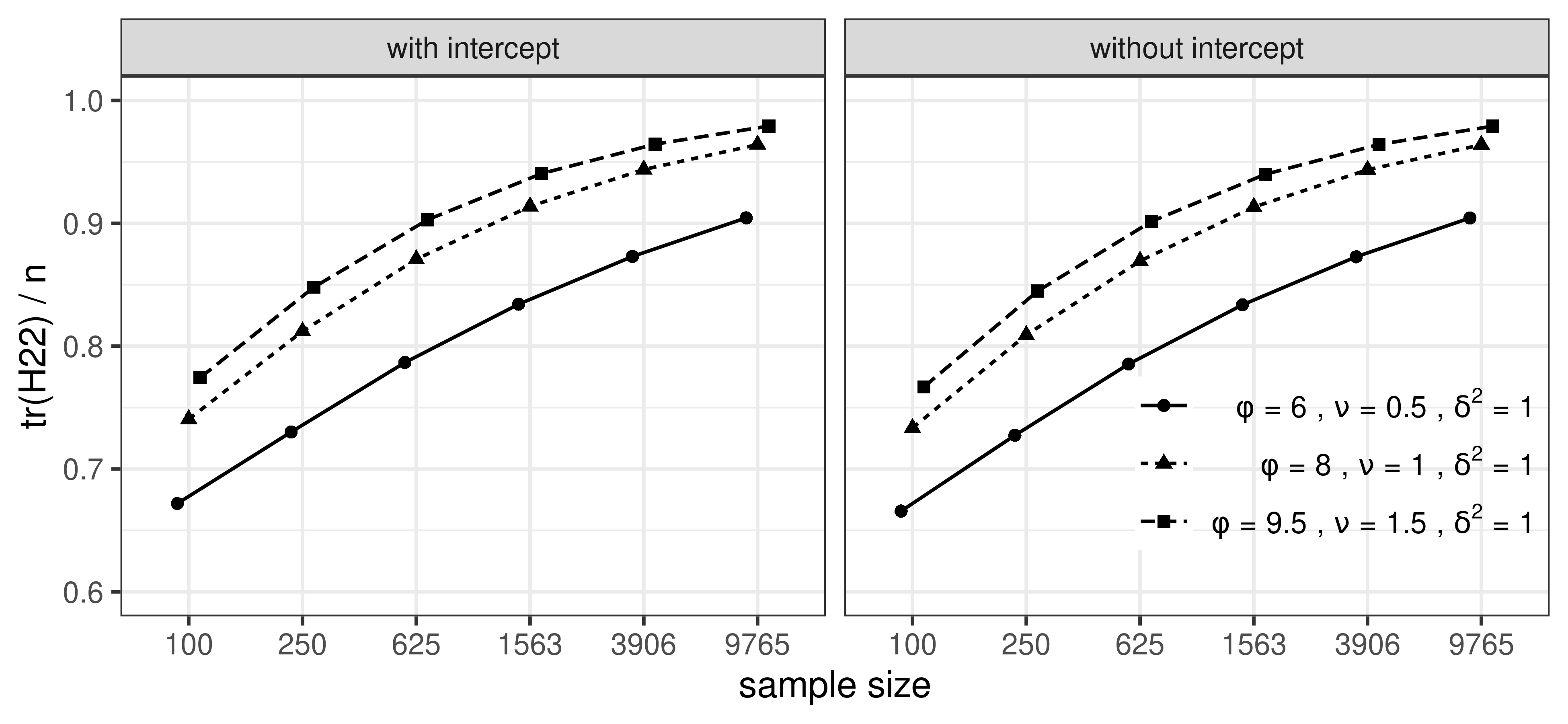
(a)

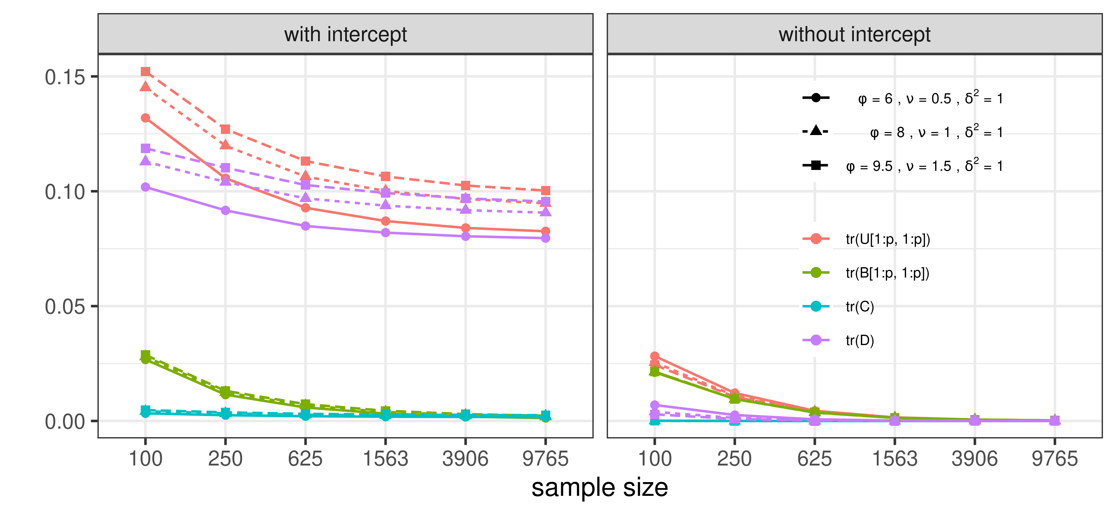
(b)

Figure 1: The top row (a) provides plots of $\operatorname{Tr}(H_{22})/n$ when $x(s)$ consists of an intercept only (left), and with additional covariates (right) for different parameter values. The bottom row (b) plots the quantities $\operatorname{Tr}\left(U_{11}\right)$, $\operatorname{Tr}\left(B_{11}\right)$, $\operatorname{Tr}(C)$, and $\operatorname{Tr}(D)$ with an intercept only (left) and with covariates (right)

Next, we consider Bayesian posterior predictive inference at a new location $s_{0}\in\mathcal{D}$. Let $Z_{n}(s_{0})$ be a random variable distributed as $p(z(s_{0})\,|\,y(\chi_{n}))$ and $Y_{n}(s_{0})$ be distributed as $p(y(s_{0})\,|\,y(\chi_{n}))$. We study the prediction error $\mathbb{E}_{0}(Z_{n}(s_{0})-z(s_{0}))^{2}$ for the latent process, and $\mathbb{E}_{0}(Y_{n}(s_{0})-y(s_{0}))^{2}$ for the response variable. Let $X_{\dagger}$ and $y_{\dagger}$ be as in (2.6) and $U$ is as in Corollary 2.5. The following theorem quantifies these posterior prediction errors.

Theorem 2.7 (Posterior predictive consistency).

Consider $s_{0}\in\mathcal{D}$. For any given $\phi>0$, denote $\operatorname{Cov}(z,z(s_{0})\,|\,\sigma^{2})$ and $R_{\phi}(\chi_{n})$ by $\sigma^{2}J_{\phi,n}$ and $R_{\phi,n}$, respectively. Let $Z_{n}(s_{0})$ have the density $p(z(s_{0})\,|\,y(\chi_{n}))$, and $Y_{n}(s_{0})$ have the density $p(y(s_{0})\,|\,y(\chi_{n}))$, and let

$$F_{n} =J_{\phi,n}^{\mathrm{\scriptscriptstyle T}}R_{\phi,n}^{-1}(U_{n}X_{\dagger}^{\mathrm{\scriptscriptstyle T}}y_{\dagger})_{[p+1:p+n]}\quad\mbox{and}\quad$$

$$G_{n} =1-J_{\phi,n}^{\mathrm{\scriptscriptstyle T}}R_{\phi,n}^{-1}(R_{\phi,n}+{U_{n}}_{[p+1:p+n,\,p+1:p+n]})R_{\phi,n}^{-1}J_{\phi,n},$$

where we use the suffix $n$ to highlight the dependency of $\chi_{n}$, and we remove the suffix $n$ of $X_{\dagger}$ and $y_{\dagger}$ when there is no confusion. Under the assumptions in Theorem 2.3, we have

$$\mathbb{E}_{0}(Z_{n}(s_{0})-z(s_{0}))^{2}=E_{1,n}+E_{2,n}+o(1),$$ (2.9)

where $\mathbb{E}_{0}$ on the left side supports $z(s_{0})$, $y(\chi_{n})$ and the external randomisation of $p(z(s_{0})\,|\,y(\chi_{n}))$, and $E_{1,n}=\mathbb{E}_{0}(z(s_{0})-F_{n})^{2}$ and $E_{2,n}=\sigma_{\alpha}^{2}G_{n}$. Moreover, if $E_{1,n},E_{2,n}\to 0$ as $n\to\infty$, then posterior inference for the latent process is consistent in the sense that $\mathbb{E}_{0}(Z_{n}(s_{0})-z(s_{0}))^{2}\to 0$ as $n\to\infty$, while posterior predictive inference for $y(s_{0})$ satisfies

$$\mathbb{E}_{0}(Y_{n}(s_{0})-y(s_{0}))^{2}\to\tau_{0}^{2}+\delta^{2}\sigma_{\alpha}^{2}\quad\mbox{as }n\to\infty.$$ (2.10)

Proof 2.8.

See Section C in the Appendix.

In the decomposition (2.9), the term $E_{1,n}$ arises in the deviation from the posterior mean, while the term $E_{2,n}$ is from the posterior uncertainty. The conditions $E_{1,n},E_{2,n}\to 0$ is analytically intractable in the general case. If, however, is we detrend the outcome so that $x(s)^{\mathrm{\scriptscriptstyle T}}\beta=0$, then $E_{1,n}$ and $E_{2,n}$ are simplified to inherit a rich structure under the Matérn covariance model for the latent process $z(s)$. In this case, we provide evidence to support the posterior predictive consistency for the latent process in the next subsection.

2.3 Conjugate Bayesian model without trend

We now consider a zero-centred spatial process for $y(s)$ at a location $s\in\mathcal{D}$ modelled as

$$y(s)=z(s)+\varepsilon(s).$$ (2.11)

Let $\mathcal{D}\subset\mathbb{R}^{d}$ be a compact domain with $d\in\{1,2,3\}$. We also assume that the correlation function $R_{\phi}(\cdot,\cdot)$ is specified by the isotropic Matérn covariogram

$$R_{\phi}(s,s^{\prime}):=\frac{(\phi|s-s^{\prime}|)^{\nu}}{\Gamma(\nu)2^{\nu-1}}K_{\nu}(\phi|s-s^{\prime}|),$$ (2.12)

where $\nu>0$ is a smoothness parameter, $\Gamma(\cdot)$ is the Gamma function, and $K_{\nu}(\cdot)$ is the modified Bessel function of the second kind of order $\nu$ (Abramowitz & Stegun, 1965, Section 10). It is known that the spectral density of the (isotropic) Matérn model without nugget is

$$f_{\mbox{\tiny Mat\'{e}rn}}(u)=C\frac{\sigma^{2}\phi^{2\nu}}{(\phi^{2}+u^{2})^{\nu+d/2}}\quad\mbox{for some }C>0.$$ (2.13)

Fix the smoothness parameter $\nu>0$, call the process (2.11) the Matérn model with parameter values $\{\sigma^{2},\phi,\tau^{2}\}$. Since there is no $x^{\mathrm{\scriptscriptstyle T}}\beta$ term, the conjugate Bayesian model (2.2) simplifies to

$$y\,|\,\sigma^{2}\sim\mathcal{N}(0,\sigma^{2}(R_{\phi}(\chi)+\delta^{2}I_{n})),\quad\sigma^{2}\sim\mbox{IG}(a_{\sigma},b_{\sigma}),$$ (2.14)

and the corresponding augmented linear regression becomes

$$\underbrace{\begin{pmatrix}y\\ 0\end{pmatrix}}_{y_{*}}=\underbrace{\begin{pmatrix}I_{n}\\ I_{n}\end{pmatrix}}_{x_{*}}z+\underbrace{\begin{pmatrix}\eta_{1}\\ \eta_{2}\end{pmatrix}}_{\eta_{*}},$$ (2.15)

where $\eta_{*}\sim\mathcal{N}(0,\sigma^{2}V_{y_{*}})$ and $V_{y_{*}}=\begin{pmatrix}\delta^{2}I_{n}&0\\ 0&R_{\phi}(\chi)\end{pmatrix}$.

The following theorem shows the posterior inconsistency of the scale $\sigma^{2}$ under the conjugate model (2.14).

Theorem 2.9 (Posterior inference for the Matérn model).

Assume that the location set $\chi=\{s_{1},\ldots,s_{n}\}$ satisfies

$$\max_{s\in\mathcal{D}}\min_{1\leq i\leq n}|s-s_{i}|\asymp n^{-\frac{1}{d}}.$$ (2.16)

Let $\mathbb{P}_{0}$ be the probability distribution of the Matérn model (2.11) with the true parameter values $(\sigma_{0}^{2},\phi_{0},\tau_{0}^{2})$. Under $\mathbb{P}_{0}$,

$$\lim_{n\to\infty}p(\sigma^{2}\,|\,y(\chi_{n}))=\delta_{\tau_{0}^{2}/\delta^{2}}\;.$$ (2.17)

Consequently, $\lim_{n\to\infty}p(\tau^{2}\,|\,y(\chi_{n}))=\delta_{\tau_{0}^{2}}$.

Proof 2.10 (of Theorem 2.9).

See Section D in the Appendix.

Note that the posterior inference of $\sigma^{2}$ is independent of the range decay $\phi$ chosen in the conjugate Bayesian model (2.14). The scale $\sigma^{2}$ is posterior inconsistent unless the noise-to-spatial variance ratio $\delta^{2}={\tau_{0}^{2}/\sigma_{0}^{2}}$, while the nugget $\tau^{2}$ is posterior consistent.

Posterior prediction for $z(\cdot)$ and $y(\cdot)$: Recall the decomposition (2.9) for the posterior prediction error for the latent process $z(s)$. The following proposition simplifies the two sources of error $E_{1,n}$ and $E_{2,n}$, when the outcome $y(s)$ follows a Matérn model in the presence of a nugget.

Theorem 2.11 (Posterior predictive consistency for the Matérn model).

Let $s_{0}\in\mathcal{D}$. Then, we have the decomposition (2.9), where $E_{1,n}$ is the prediction error of the best linear predictor for a Matérn model with parameters $\{\sigma^{\prime 2},\phi,\tau^{\prime 2}\}$ satisfying $\delta^{2}=\frac{\tau^{\prime 2}}{\sigma^{\prime 2}}$, and

$$E_{2,n}:=\frac{\tau_{0}^{2}}{\delta^{2}}\left[1+J_{\phi,n}^{\mathrm{\scriptscriptstyle T}}\left\{(I_{n}+\delta^{-2}R_{\phi}(\chi_{n}))^{-1}-I_{n}\right\}R_{\phi}(\chi_{n})^{-1}J_{\phi,n}\right].$$ (2.18)

Moreover, if $E_{1,n},E_{2,n}\to 0$ as $n\to\infty$, then the latent process $z(s)$ is posterior predictive consistent in the sense that $\mathbb{E}_{0}(Z_{n}(s_{0})-z(s_{0}))^{2}\to 0$ as $n\to\infty$ and, hence, $\mathbb{E}_{0}(Y_{n}(s_{0})-y(s_{0}))^{2}\to 2\tau_{0}^{2}$ as $n\to\infty$.

Proof 2.12.

See Section E in the Appendix.

Theorem 2.11 reveals that the posterior mean of the conjugate Bayesian model (2.14) is identified as the best linear predictor of any Matérn model with parameters $\{\sigma^{\prime 2},\phi,\tau^{\prime 2}\}$ provided $\tau^{\prime 2}/\sigma^{\prime 2}=\delta^{2}$. This observation connects the Bayesian modelling to a frequentist approach in that the deviation error $E_{1,n}$ is viewed as the prediction error of the best linear predictor of a Matérn model in the presence of a nugget. Next we provide evidence to support the posterior predictive consistency for the latent process in the sense that $E_{1,n},E_{2,n}\to 0$ as $n\to\infty$.

The deviation error $E_{1,n}$: It is expected that the prediction error of the best linear predictor of a Matérn model in the presence of a nugget tends to $0$ as long as the fill distance condition (2.16) holds. However, it is hard to prove this statement in the general case. To provide some ideas, we consider a particular one-dimensional example.

We assume without loss of generality that $\mathcal{D}=[-1,1]$, and $\chi=\{i/n,\,-n\leq i\leq n\}$ so the fill distance condition (2.16) is satisfied. Also let $\chi_{\infty}=\{i/n,\,-\infty<i<\infty\}$ be the infinite evenly spaced grid. Define

$$\widehat{z}:=\mathbb{E}(z(0)\,|\,y(s),s\in\chi\setminus\{0\})\quad(\mbox{resp. }\widehat{z}_{\infty}:=\mathbb{E}(z(0)\,|\,y(s),s\in\chi_{\infty}\setminus\{0\})),$$

be the best linear predictor of $z(0)$ based on the observations $y(s)$ on $\chi\setminus\{0\}$ (resp. $\chi_{\infty}\setminus\{0\}$). Note that $\widehat{z}$ (resp. $\widehat{z}_{\infty}$) may well be computed using misspecified parameter values $\{\phi,\delta^{2}\}$. Let

$$e:=\mathbb{E}_{0}(z(0)-\widehat{z})^{2}\quad(\mbox{resp. }e_{\infty}:=\mathbb{E}_{0}(z(0)-\widehat{z}_{\infty})^{2}),$$ (2.19)

be the prediction error of the best linear predictor based on the observations on the finite grid $\chi\setminus\{0\}$ (resp. the infinite grid $\chi_{\infty}\setminus\{0\}$). We make the following assumption which relates $e$ to $e_{\infty}$ as $n\to\infty$.

[Infinite approximation] The difference $e-e_{\infty}\to 0$ as $n\to\infty$.

Basically, this assumption suggests that as the grid becomes finer and finer, observations outside any fixed bounded interval have little impact on the prediction of $z(0)$. However, it is not easy to prove such a statement which is conjectured in (Stein, 1999, page 97). The plan is to prove $e_{\infty}\to 0$, and by Assumption 2.12 it implies that $e\to 0$ as $n\to\infty$. This program is recorded in the following proposition.

Proposition 2.13 (Prediction error for the Matérn model).

Let $\mathcal{D}=[-1,1]$ and $\chi=\{i/n,\,-n\leq i\leq n\}$. Under Assumption 2.12, we have

$$e\longrightarrow 0\quad\mbox{as }n\to\infty,$$ (2.20)

where $e$ is the prediction error of the best linear predictor defined as in (2.19).

Proof 2.14.

See Section F in the Appendix.

The posterior variance $E_{2,n}$: The error term $E_{2,n}$ defined by (2.18) is also analytically intractable. Here, we provide a numerical study to investigate the behaviour of $E_{2,n}$ when $n\to\infty$ in the general case. We first generate the location set $\chi$ by uniformly sampling $n$ locations in $[0,1]$ or $[0,1]^{2}$, then we compute $E_{2,n}$ for every location in $\chi$ with $\delta^{2}=1,\tau^{2}=1$ and different values of $\phi$ and $\nu$. We expand the location set $\chi$ sequentially to sets with larger sample sizes by adding locations that are uniformly sampled in the study domain. For each expanded set $\chi$, we recompute the $E_{2,n}$ for all locations in $\chi$. Figure 2 plots the median, the 2.5th and 97.5th percentiles of $E_{2,n}$ for different sample sizes. The values of $E_{2,n}$ for points in a fixed domain, shown in Figure 2, decrease rapidly as the sample size increases, although the rate diminishes when $d$ increases from $1$ to $2$. This suggests that the decreasing rate is related to dimension.

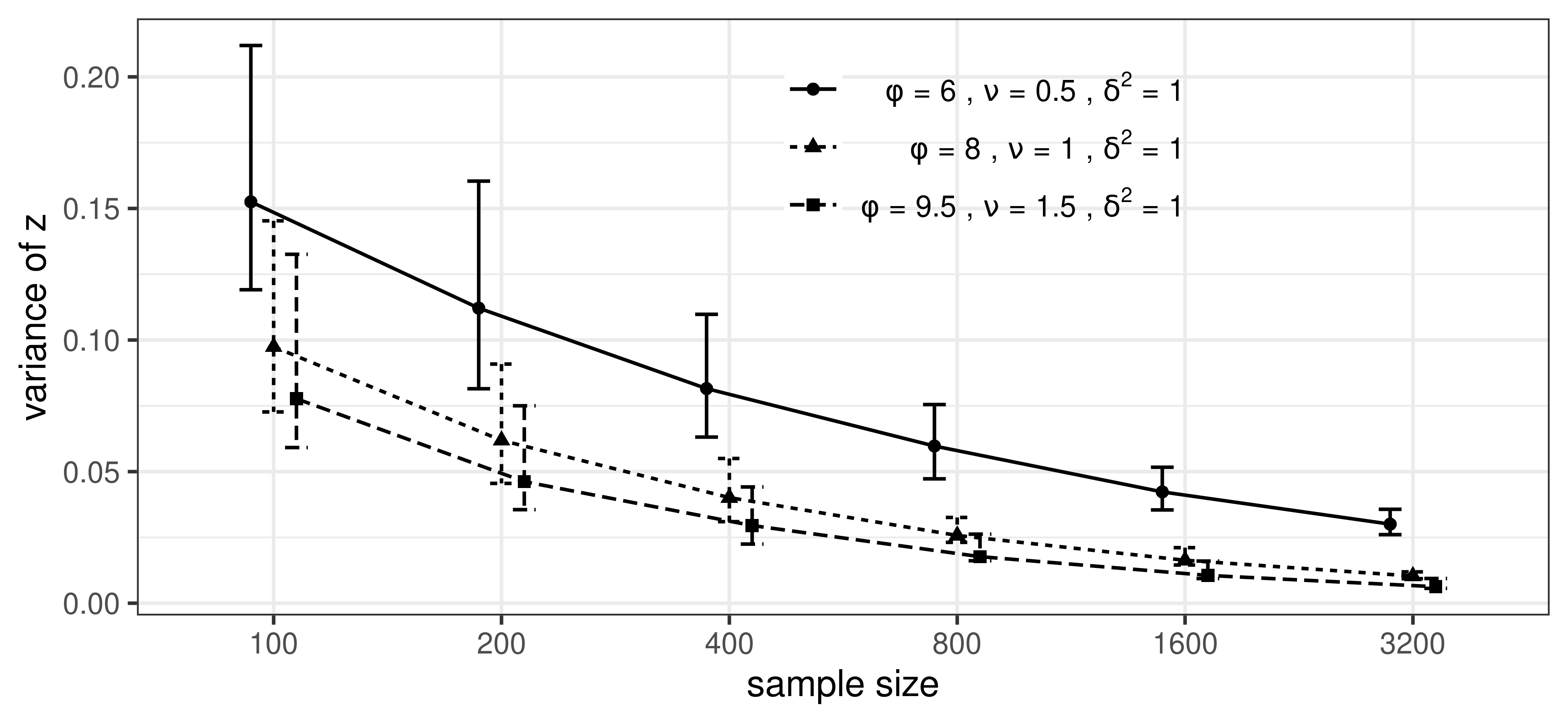
(a)

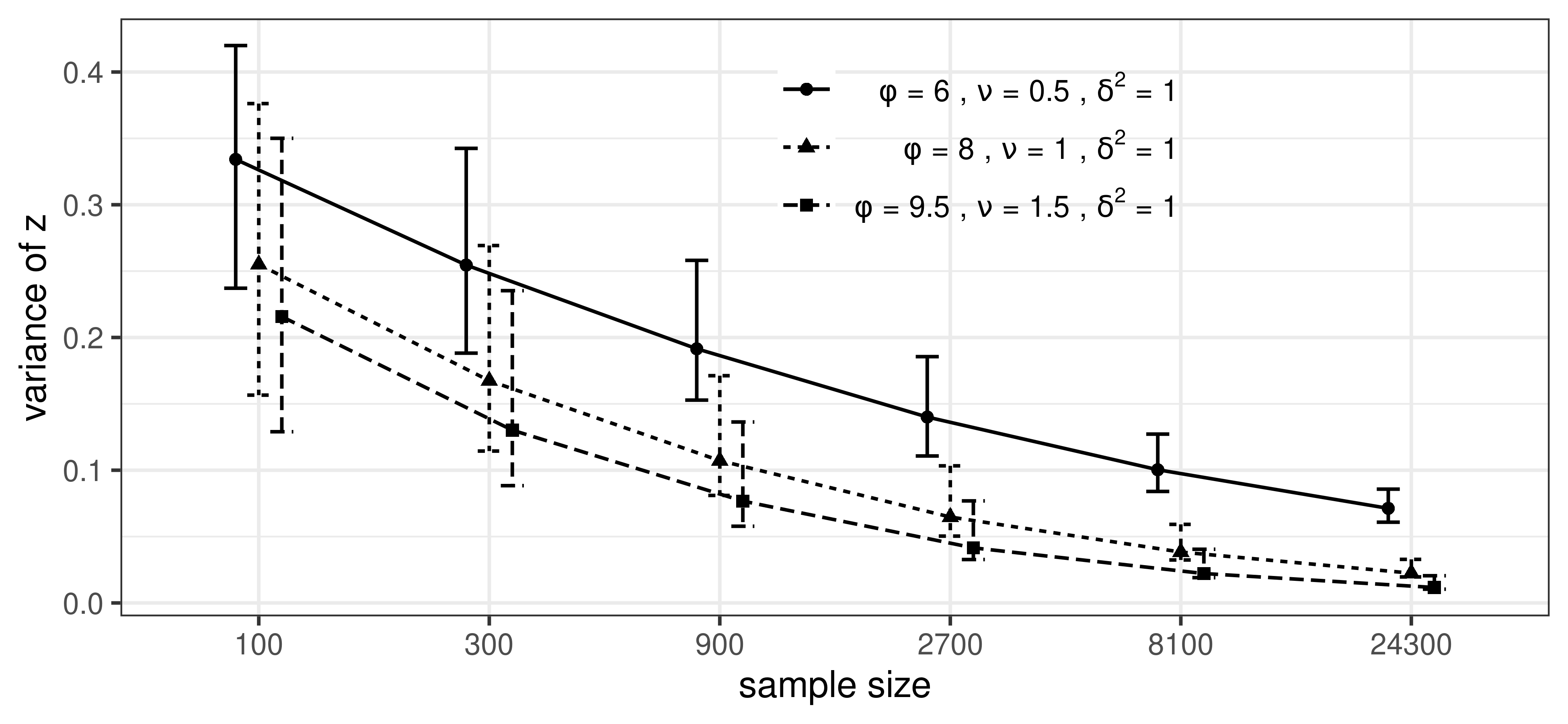
(b)

Figure 2: The median of $E_{2,n}$ for locations uniformly sampled on $[0,1]$ (a) and $[0,1]^{2}$ (b). The error bars indicate the 97.5th and 2.5th percentiles. The sample size $n$ ranges from 100 to 3,200 and from 100 to 24,300 for the experiments on $[0,1]$ and $[0,1]^{2}$, respectively.

3 Stacking algorithms for spatial models

3.1 Stacking of means

The Bayes predictor for $\tilde{y}(s_{0})$ under model $M_{g}$, for each $g=1,\ldots,G$, is $\mathbb{E}_{g}(\tilde{y}(s_{0})\,|\,y)=\int\tilde{y}(s_{0})p(\tilde{y}(s_{0})\,|\,y,M_{g})d\tilde{y}(s_{0})$, where $\mathbb{E}_{g}(\tilde{y}(s_{0})\,|\,y)$ is the expectation of the posterior predictive mean computed from $M_{g}$. Stacking methods will combine the $G$ Bayes predictors as a weighted average

$$\sum_{g=1}^{G}w_{g}\mathbb{E}_{g}(\tilde{y}(s_{0})\,|\,y),$$ (3.1)

where $\{w_{1},\ldots,w_{G}\}$ are the weights for combination. Define the leave-one-out (LOO) Bayes predictor for $\tilde{y}(s_{i})$ under model $M_{g}$ as

$$\hat{y}_{g}(s_{i})=\mathbb{E}_{g}(\tilde{y}(s_{i})\,|\,y_{-i},M_{g}) =\int\int\tilde{y}(s_{i})p(\tilde{y}(s_{i})\,|\,\theta,M_{g})p(\theta\,|\,y_{-i},M_{g})d\theta d\tilde{y}(s_{i})$$

where $y_{-i}$ is the data without the $i$th observation. Stacking determines the optimal weights as

$$\operatorname{\arg\min}_{w}\sum_{i=1}^{n}\left(y(s_{i})-\sum_{g=1}^{G}w_{g}\hat{y}_{g}(s_{i})\right)^{2}\;.$$ (3.2)

The following proposition studies the posterior prediction error using the stacking predictor, where we only require that the weights be bounded.

Proposition 3.1.

Let $s_{0}\in\mathcal{D}$, and $w^{*}:=(w^{*}_{1},\ldots,w^{*}_{G})$ be the stacking weights defined by (3.2) such that $|w^{*}_{g}|$ is bounded for each $1\leq g\leq G$. Let the assumptions in Theorem 2.7 or Theorem 2.11 hold for each model $M_{g}$. We have

$$\mathbb{E}_{0}\left(y(s_{0})-\sum_{g=1}^{G}w^{*}_{g}\mathbb{E}_{g}(y(s_{0})\,|\,y)\right)^{2}\to\tau_{0}^{2}\quad\mbox{as }n\to\infty.$$ (3.3)

Proof 3.2.

See Section G in the Appendix.

The following theorem shows that the stacking predictor asymptotically minimises the posterior prediction error.

Theorem 3.3.

Let $s_{0}\in\mathcal{D}$, and $w^{*}:=(w^{*}_{1},\ldots,w^{*}_{G})$ be the stacking weights defined by (3.2) such that $|w^{*}_{g}|$ is bounded for each $1\leq g\leq G$. Let

$$E_{1,g,i}:=\mathbb{E}_{0}(z(s_{i})-\widehat{y}_{g}(s_{i}))^{2},\quad 1\leq g\leq G\mbox{ and }1\leq i\leq n,$$

be the deviation error for the latent process $z(s)$ by leaving the $i^{th}$ observation out under the model $M_{g}$. Assume that for each $1\leq g\leq G$,

$$\frac{1}{n}\sum_{i=1}^{n}E_{1,g,i}\to 0\quad\mbox{as }n\to\infty.$$ (3.4)

Also, if the assumptions in Theorems 2.7 or 2.11 hold for each model $M_{g}$, then as $n\to\infty$ we obtain

$$\mathbb{E}_{0}\left(y(s_{0})-\sum_{g=1}^{G}w^{*}_{g}\mathbb{E}_{g}(y(s_{0})\,|\,y)\right)^{2}-\mathbb{E}_{0}\left(\frac{1}{n}\sum_{i=1}^{n}\left(y(s_{i})-\sum_{g=1}^{G}w^{*}_{g}\hat{y}_{g}(s_{i})\right)^{2}\right)\to 0.$$ (3.5)

Proof 3.4.

See Section H in the Appendix.

Equation (3.4) implies that for each model $M_{g}$ the average deviation error for the latent process goes to $0$ as the sampling resolution becomes finer. This condition is consistent with the fact that in the one-dimensional grid we typically have $E_{1,g,i}\asymp\Delta^{\min(2\nu_{0},\frac{2\nu}{2\nu+1})}$ (see Proposition 2.13); hence $\frac{1}{n}\sum_{i=1}^{n}E_{1,g,i}\to 0\to 0$ as $n\to\infty$.

Theorem 3.3 holds for candidate models with a misspecified smoothness parameter $\nu$ in the Matérn kernel for $d=1$. Note that Clyde & Iversen (2013, p.487) proves a similar result, while the established theoretical results about stacking assume exchangeability which is not available in geostatistical models. The innovation in our theoretical results emerge from studying the behaviour of the posterior and predictive distributions within the infill asymptotic paradigm. The proof of Theorem 3.3 can be extended to the case where the LOO Bayes prediction $\hat{y}_{g}(s_{i})$ is replaced by a much cheaper prediction based on $K$-fold cross-validation.

3.2 Stacking of predictive densities

Following the generalised Bayesian stacking framework established in Yao et al. (2018), we devise a second stacking algorithm for spatial analysis, which we refer to as stacking of predictive densities. This algorithm finds the distribution in the convex hull ${\cal C}=\{\sum_{g=1}^{G}w_{g}\times p(\cdot\,|\,M_{g}):\sum_{g}w_{g}=1,w_{g}\geq 1\}$ that is optimal according to some proper scoring functions. Here $p(\cdot\,|\,M_{g})$ refers to the distribution of interest under model $M_{g}$. Let ${{\mathcal{S}}}_{1}^{G}=\{w\in[0,1]^{G}:\sum_{g=1}^{G}w_{g}=1\}$ and $p_{t}(\cdot\,|\,y)$ be the true posterior predictive distribution. Using the logarithmic score (corresponding to the KL divergence), we seek $w$ so that

$$\underset{w\in{\mathcal{S}}_{1}^{G}}{\mbox{max}}\frac{1}{n}\sum_{i=1}^{n}\log\left(\sum_{k=1}^{G}w_{g}p(y(s_{i})\,|\,y_{-i},M_{g})\right)\;.$$ (3.6)

The optimal distribution $\sum_{g=1}^{G}w_{g}p(y(s_{i})\,|\,y_{-i},M_{g})$ provides a “likelihood” of observing $y(s_{i})$ on location $s_{i}$ given other data. Therefore, $\prod_{i=1}^{n}\sum_{g=1}^{G}w_{g}p(y(s_{i})\,|\,y_{-i},M_{g}))$ serves as a pseudo-likelihood that measures the performance of prediction based on the weighted average of the LOO predictors for all observed locations. Also, it provides an approximation of the expected log point-wise predictive density (ELPD)

$$\sum_{i=1}^{N}\int p_{t}(y(s_{i}))\log\left(\sum_{g=1}^{G}w_{g}p(y(s_{i})\,|\,y_{-i},M_{g})\right)dy(s_{i})$$ (3.7)

It is worth pointing out that the weights for stacking of means are not necessarily positive, while those for stacking of predictive densities must be non-negative. Relaxing this restriction imparts greater flexibility in prediction and improves prediction accuracy for stacking of means. On the other hand, we can no longer interpret negative weights as a reflection of our prior beliefs regarding $\psi$. In our subsequent experiments, we restrict the stacking weights for both algorithms to be non-negative so that the diagnostic metric MLPD (the average log pointwise predictive density, introduced in Section 4) is valid for both algorithms.

3.3 Predictive stacking in finite sample spatial analysis

A critical step in solving stacking weights is the computation of the Bayes predictor and predictive density. Computing the exact LOO Bayes predictor and predictive densities for all observed locations $\{s_{1},\ldots,s_{n}\}$ requires refitting a model $n$ times. For a Gaussian latent variable model with the number of parameters larger than the sample size $n$, there are limited choices for approximating LOO predictors accurately without the onerous computation (see, e.g., Vehtari et al., 2016). Instead of the LOO cross-validation, we prefer using the much cheaper $K$-fold cross-validation to generate the predictions. Using $K$-fold cross-validation instead of LOO in stacking is first implemented in Breiman (1996b), where the simulation evinces that $10$-fold cross-validation can provide more efficient predictors than LOO cross-validation. Here, we use $K=10$ in the implementations in Section 4.

We offer the pseudo-code algorithms for stacking of means and stacking of predictive densities using the conjugate Bayesian spatial regression model in Section I. In the algorithms, we first partition the data into $K$-folds based on locations. Letting $X=[x(s_{1}):\cdots:x(s_{n})]^{\mathrm{\scriptscriptstyle T}}$ be the design matrix, we use $X[k]$, $y[k]$, $\chi_{n}[k]$ to denote the predictors, response and observed locations from $k$-th fold, respectively, and $X[-k]$, $y[-k]$ $\chi_{n}[-k]$ to denote the respective data not in $k$-th fold. The values of the prefixed hyper-parameters $\{\phi,\nu,\delta^{2}\}$ of the conjugate Bayesian spatial regression model are picked from the grid $G_{all}$, which is expanded over the grids of candidate values as the cartesian product $G_{\phi}\times G_{\nu}\times G_{\delta}^{2}$ for $\{\phi,\nu,\delta^{2}\}$. For stacking of means, we compute the expected latent process $z_{(\phi,\nu,\delta^{2})}^{(k)}$ on locations in fold $k$ for each $\{\phi,\nu,\delta^{2}\}$ from $G_{all}$ and then generate the corresponding expectation $y_{(\phi,\nu,\delta^{2})}^{(k)}$ to obtain the stacking weights.

For stacking of predictive densities, we compute the log point-wise predictive density, ($lp_{(\phi,\nu,\delta^{2})}(s)$), of $y(s)$ at location $s$ for locations in each fold for all candidate models to find the stacking weights. The closed form of the log point-wise predictive density is derived in Section J of the Appendix. We also devise a Monte Carlo algorithm for stacking of predictive densities, which is expounded in Section K of the Appendix. Solving the weights for stacking of means is a quadratic programming problem. We use the solve.QP() function offered by the quadprog package in the R statistical computing environment and the solver Mosek to solve the weights in our R and Julia implementations, respectively. The stacking weights for stacking of predictive densities are calculated by Mosek in both our R and Julia implementations.

4 Simulation

4.1 Simulation settings

We present two simulations to examine the predictive performance of the proposed stacking algorithms. The data sets for experiments are generated by model (2.1) on locations sampled uniformly over a unit square $[0,1]^{2}$, where the correlation function $R_{\phi}$ is specified by the Matérn covariogram (2.12). The sample size $n$ of the simulated data sets ranges from $200$ to $900$, and we randomly pick $n_{h}=100$ observations for checking predictive performance. The vector $x(s)$ consists of an intercept and a single predictor generated from a standard normal distribution. The true value of the parameters for generating the data in the first simulation are $\beta=(1,2)^{\mathrm{\scriptscriptstyle T}}$, $\phi=7$, $\sigma^{2}=1$, $\tau^{2}=1$ and $\nu=1$. In the second simulation, we alter the hyper-parameters in the Matérn covariogram to $\phi=20$, $\sigma^{2}=1$, $\tau^{2}=0.3$ and $\nu=0.5$.

We consider customary values of smoothness in spatial analysis, $\nu\in G_{\nu}=\{0.5,1,1.5,1.75\}$. The candidate values for $\phi$ are selected so that the “effective spatial range”, which refers to the distance where spatial correlation drops below 0.05, covers $0.1$ and $0.6$ times $\sqrt{2}$ (the maximum inter-site distance within a unit square) for all candidate values of $\nu$. Here we set $G_{\phi}=\{3,14,25,36\}$. Finally, we specify $G_{\delta^{2}}=\{0.1,0.5,1,2\}$ as the candidate grid for $\delta^{2}$. We assign an $\mbox{IG}(a_{\sigma},b_{\sigma})$ prior with $a_{\sigma}=b_{\sigma}=2$ for $\sigma^{2}$. The prior of $\beta$ follows a zero centred Gaussian with the covariance matrix equal to a diagonal matrix whose diagonal elements are $4$, i.e., $\mbox{N}(\mu_{\beta},V_{\beta})$ where $\mu_{\beta}=\mathbf{0}$ and $V_{\beta}=4\cdot{I}$. For each simulated data set, we use stacking of means and stacking of predictive densities to obtain the expected outcome $\hat{y}(s)$ based on the held out observed locations. The predictive accuracy is evaluated by the mean squared prediction error over a set of $n_{h}$ hold-out locations in set ${\cal S}_{h}$ ($\text{MSPE}=\sum_{s\in{\cal S}_{h}}((\hat{y}(s)-y(s))^{2})/n_{h}$). We also compute the posterior expected values of the latent process $\hat{z}(s)$ for $z(s)$ on all of the $n$ sampled locations in ${\cal S}$ and evaluate the mean squared error for $z(s)$ ($\text{MSEZ}=\sum_{s\in{\cal S}}(\hat{z}(s)-z(s))^{2}/n$). To further evaluate the distribution of predicted values, we compute the mean log point-wise predictive density for the $n_{h}$ held out locations ($\text{MLPD}=\sum_{s\in{\cal S}_{h}}\{\log(\sum_{g=1}^{G}w_{g}p(y(s)\,|\,y,M_{g}))\}/n_{h}$).

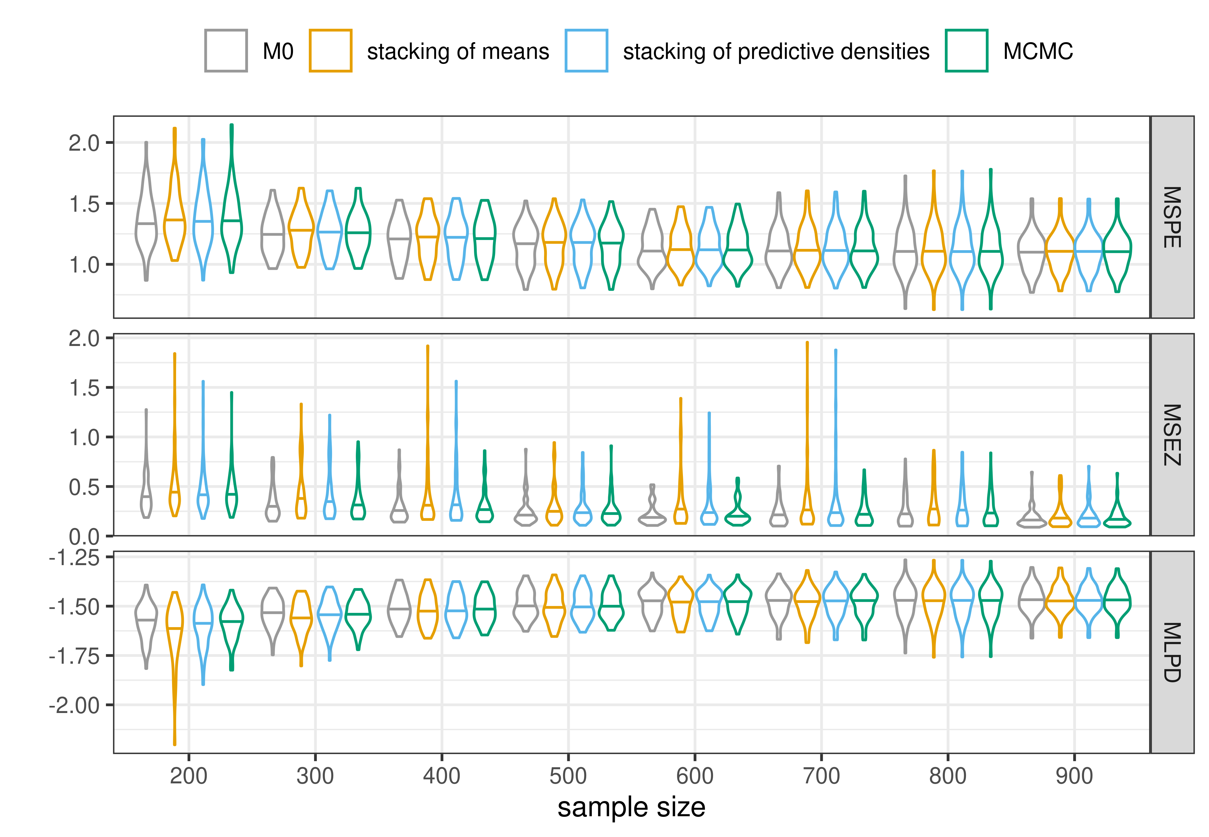
(a)

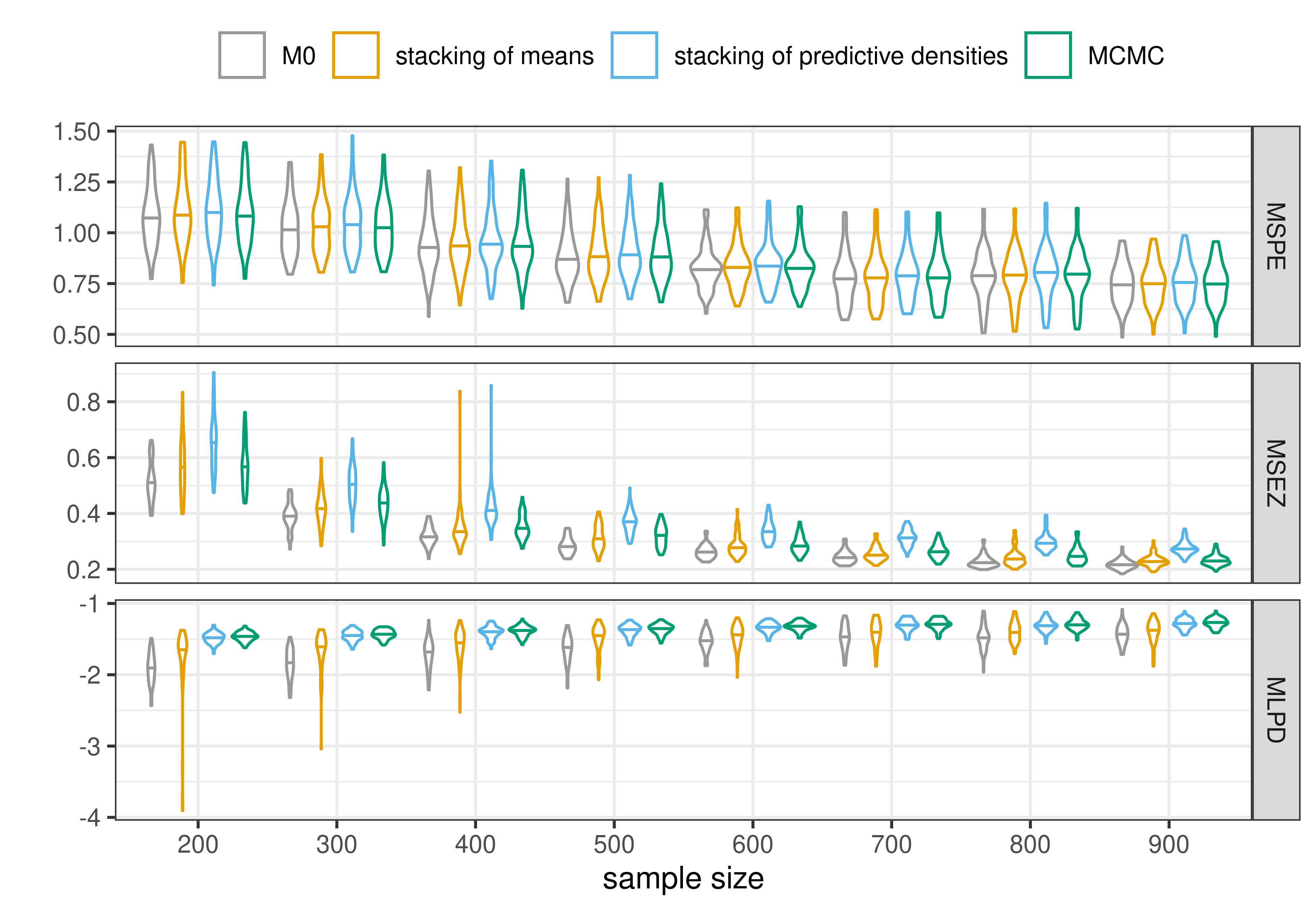
(b)

Figure 3: Distributions of the diagnostic metrics for prediction performance for the first simulation (a) and the second simulation (b). Each distribution is depicted through a violin plot. The horizontal line in each violin plot indicates the median.

Apart from stacking, we also implemented a fully Bayesian model with priors on the hyperparameters using Markov chain Monte Carlo (MCMC) sampling for comparison. In addition, we carried out exact Bayesian inference using the conjugate model in Section 2.1 with hyper-parameters fixed at the exact value (denoted as $M_{0}$). We use the same priors for $\sigma^{2}$ and $\beta$ as those in stacking implementations. For the rest of the priors needed in full MCMC sampling, we assign uniform priors $\mbox{U}(3,36)$ for $\phi$ and $\mbox{U}(0.25,2)$ for $\nu$, and an $\mbox{IG}(2,2)$ prior for $\tau^{2}$. Sampling is fitted through the spLM function in the spBayes package in R. The diagnostic metrics are computed based on 1,000 posterior samples retained after convergence was diagnosed over a burn-in period of 10,000 initial iterations. The algorithm for recovering the expected $z$ and the log point-wise predictive density based on the output of spLM is presented in Section L of the Appendix. We monitor all diagnostic metrics for prediction for all competing algorithms. To measure uncertainty of the diagnostic metrics, we generate 60 data sets for each sample size in each simulation, fit each data set with the four competing methods and record the diagnostic metrics of each model fitting.

4.2 Predictive performances

Interestingly, the candidate algorithms exhibit different behaviours in the two simulation studies. Figure 3 summarises the comparison of the predictive performance. In the first simulation there seem to be no pronounced distinctions between the prediction performance for all competing models. In the second simulation, however, we observe that stacking of means outperforms stacking of predictive densities on having better estimates of the latent process on both the observed and unobserved locations (based on MSEZ), while stacking of predictive densities outperforms stacking of means in terms of the log point-wise predictive density (based on MLPD). These results are expected since we optimise the prediction error in the stacking of means, and we maximise the log predictive densities in the stacking of predictive densities.

Treating the fully Bayesian model with priors on all hyperparameters (fitted using MCMC) as a benchmark, we find that stacking of predictive densities is very competitive in terms of MLPD. The performance of latent process estimation for the full Bayesian model falls between stacking of means and stacking of predictive densities. The prediction accuracy for the response on unobserved locations for all competing algorithms are very close. Based on the medians of the MSPEs for all fittings, stacking of means slightly outperforms the full Bayesian model, and both are slightly better than stacking of predictive densities, The conjugate Bayesian model $M_{0}$ provides the best point estimates for both response and latent processes based on MSPE and MSEZ, while it performs worse in terms of MLPD. These results seem to indicate that, when choosing stacking algorithms, stacking of means is preferred for point estimation and stacking of predictive densities is preferable for interval estimation.

In Figure 4, we compare the counts of the non-zero weights in stacking and find that stacking of means tends to produce a slightly smaller number of non-zero weights than stacking of predictive densities. The number of non-zero weights is small for both stacking algorithms, and this phenomenon is also observed and discussed in Breiman (1996b). On average, there are around 3.7 and 4.5 out of 64 weights that are greater than 0.001 in the simulation studies for stacking of means and stacking of predictive densities, respectively. And the number is relatively consistent when the sample sizes increase. These results suggest that stacking methodology is memory efficient, which is beneficial for large-scale spatial data analysis.

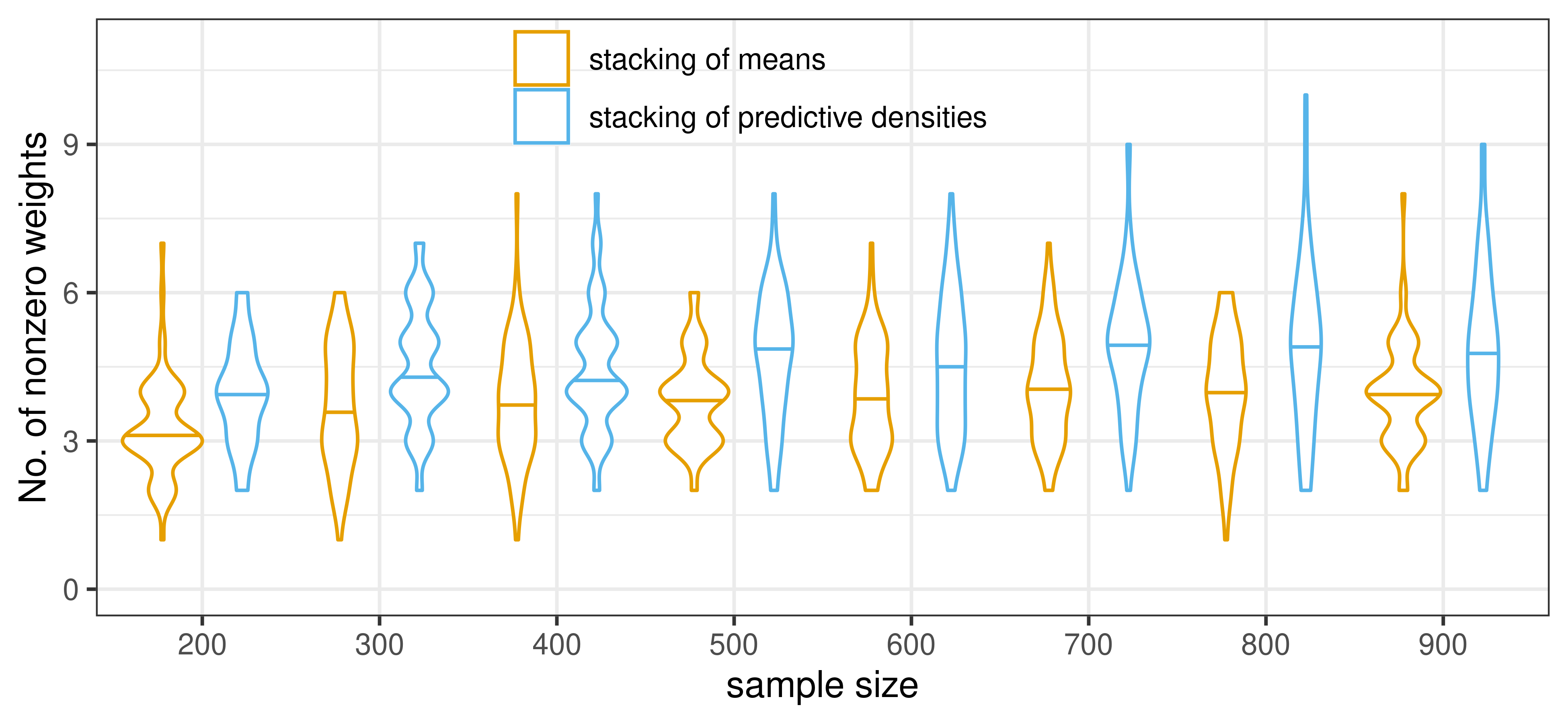
(a)

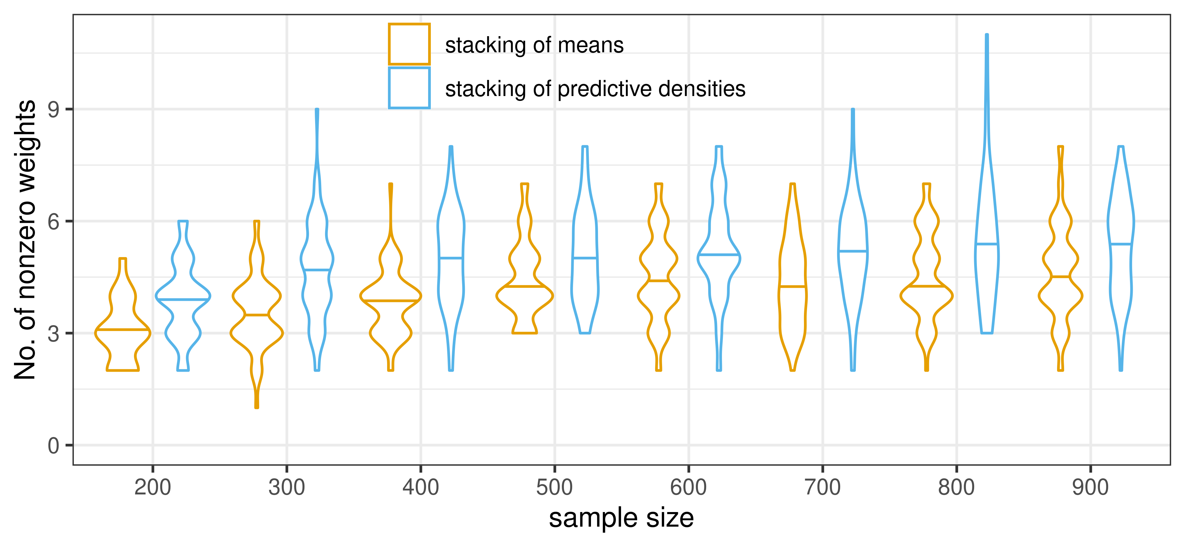
(b)

Figure 4: Distributions of the counts of nonzero weights in the first (a) and the second (b) simulation. The distribution of the counts are described through violin plots whose horizontal lines indicate the medians.

In Section M.1, we pick one run for each simulation study and illustrate the interpolated maps of the predicted response on held out locations and expected latent processes over all locations generated by different fitting algorithms. The predicted response resembles the de-noised response ($x(s)^{\mathrm{\scriptscriptstyle T}}\beta+z(s)$, not $y(s)$), and the estimated latent process shares a similar pattern with the raw data. The latent process estimated by stacking of predictive densities is observed to be slightly smoother than those estimated by other algorithms, while the predictions of the response on unobserved locations fitted by different fitting algorithms are almost indistinguishable.

4.3 Running time comparisons

We provide both R and Julia code for the two proposed stacking algorithms. The code for the simulation studies are available from the GitHub repository https://github.com/LuZhangstat/spatial_stacking. Comparisons in predictive performances presented above are conducted in R. For the running time comparisons reported here, the stacking algorithms are implemented using Julia-1.6.6 and the MCMC sampling algorithms are run in R-4.2.0. We report the time for obtaining weights for stacking, and we consider the sampling time for $\{\phi,\nu,\sigma^{2},\tau^{2}\}$ using MCMC (no sampling of $\{\beta,z\}$ and no predictions). The timing comparisons are based upon experiments on a Windows 10 pro platform, with 64 GB of RAM and a 1-Intel Core i7-7700K CPU @ 4.20GHz processor with 4 cores each and 2 threads per core—totalling 8 possible threads for parallel computing. Figure 5 summarises the running time for the three competing algorithms. On average, the stacking of means is 526 times faster than MCMC in the simulation study. Stacking of predictive densities is slightly slower than stacking of means but is still around 430 times faster than MCMC sampling. These experiments clearly establish that predictive stacking algorithms are efficient alternatives to the full MCMC sampling algorithms for estimating latent spatial processes and predicting geostatistical outcomes.

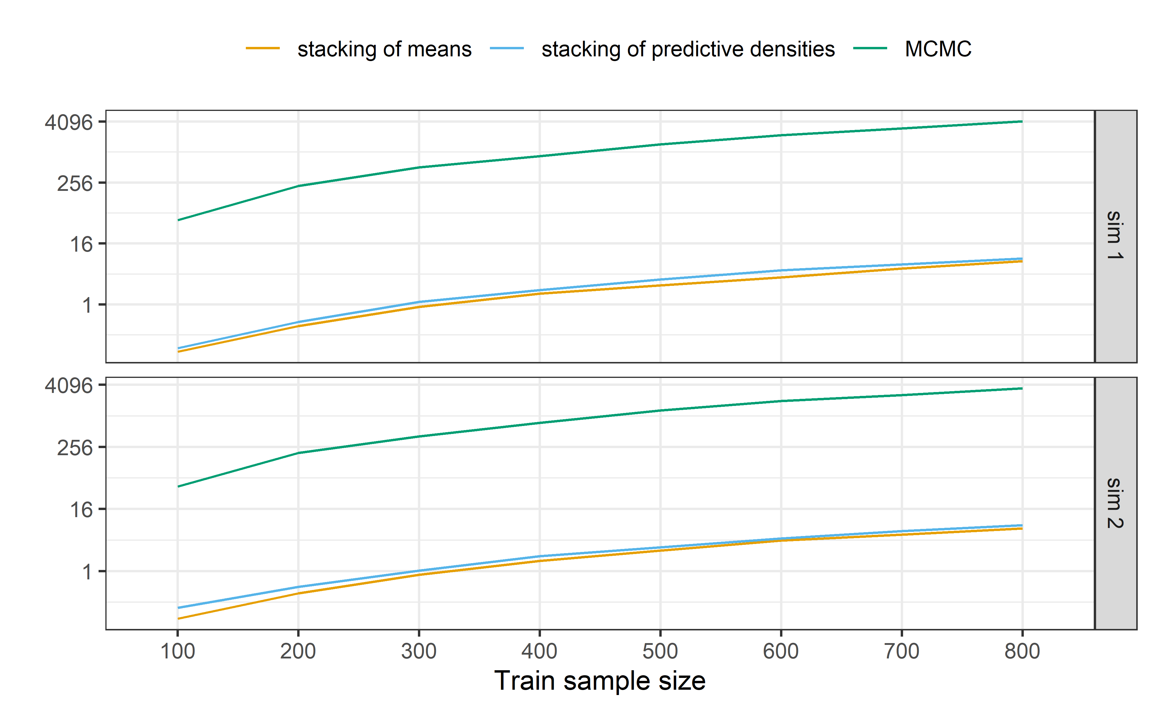
Figure 5: Running time comparison for stacking and MCMC sampling

4.4 Inference of prefixed hyper-parameters

One limitation of stacking, compared to full Bayesian inference (e.g., using MCMC sampling algorithms), is that it does not provide interval estimates for the prefixed hyper-parameters. Moreover, our experiments show that stacking cannot provide a reliable point estimate of the hyper-parameters. If we treat the grid of the candidate values for the hyper-parameters in our stacking algorithms as a discrete uniform prior, then, intuitively, we should be able to achieve point estimates for those fixed hyper-parameters by a weighted average based on stacking weights. In Figure 6, we compare the point estimates of $\phi$ based on stacking for the simulation studies. It is clear that stacking of means yields unstable estimates. Stacking of predictive densities has a smaller variance, but the bias can be large. Meanwhile, since $\phi$ is not identifiable, we observe that the posterior interval estimates for $\phi$ inferred from MCMC algorithms are wide, showing that the inference for $\phi$ is relatively unstable for all candidate algorithms in this simulation study. The comparisons of the other two hyper-parameters are provided in the Section M.2.

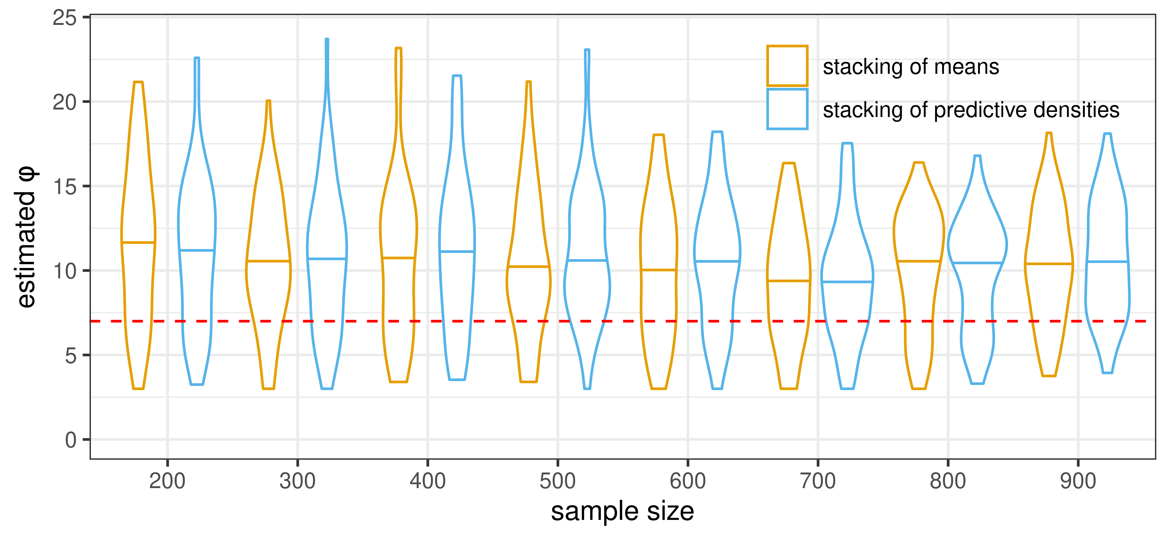
(a)

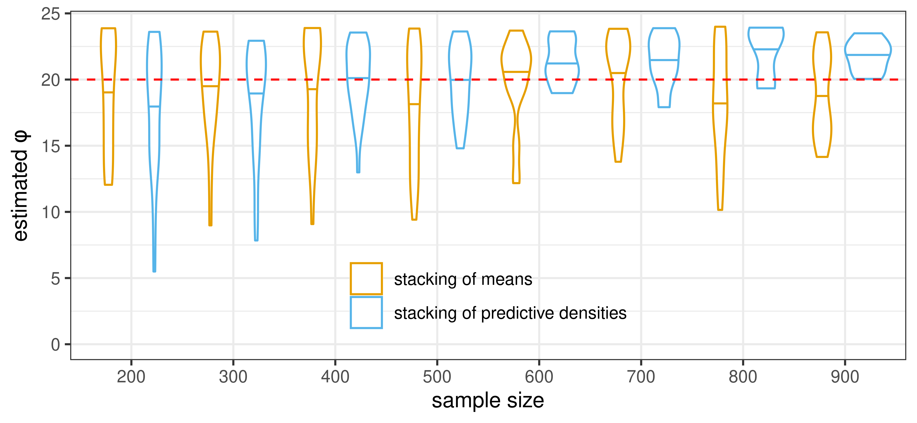
(b)

Figure 6: Distributions of the estimated $\phi$ in the first (a) and the second (b) simulation. The distribution of the counts are described through violin plots whose horizontal lines indicate the medians. The red dashed horizontal line indicates the actual value of $\phi$

5 Western experimental forest inventory data analysis

We illustrate our proposed stacking methodology using the Western Experimental Forest (WEF) inventory data from a long-term ecological research site in western Oregon. This data set contains coordinates, species, diameter at breast height (DBH) and other measurements for trees in the experimental forest. The raw data is provided in the R package spBayes, and the code is available from the GitHub repository https://github.com/LuZhangstat/spatial_stacking. In this analysis, we focus on the prediction of DBH for living trees using the location and species information. There are 1,954 records in all after cleaning up some of the data. We randomly hold out 500 points for prediction and use the remaining observations to train the model and draw posterior inference.

We first fit a Bayesian linear regression model (BLM) using Hamiltonian Monte Carlo algorithms implemented in the Stan Bayesian modelling environment through the R interface rstanarm. We run the model fitting with the default settings, where the default priors are described in Gabry & Goodrich (2020). Then, we use the same prior for $\beta$ in our stacking implementations. For the prior of $\sigma^{2}$ in stacking implementations, we set up the hyper-parameters in the inverse-Gamma to have mean at the square of the mean of the default prior for $\sigma$ in BLM. We use the same candidate values for $\nu$ and $\delta^{2}$ as our simulation studies in Section 4. The largest and smallest candidate values for $\phi$ are the maximum and minimum values so that the effective spatial range covers 0.1 and 0.6 times the maximum inter-site distance for Matérn covariogram with all candidate smoothness $\nu$ values. We pick four candidate values for $\phi$ in this data analysis. Finally, we evaluate predictive performance using the root mean squared prediction error (square root of the MSPE defined in Section 4.1) and the average log point-wise predictive density (MLPD defined in Section 4.1) for all held out locations. Table 1 summarises the result. Stacking delivers an RMSPE that is lower by around 9% and yields better MLPD in this data analysis.

Table 1: Summary Statistics of Western experimental forest inventory data analysis

	Bayesian linear regression	stacking of means	stacking of predictive densities
RMSPE	22.86	20.70	20.79
MLPD	-4.55	-4.45	-4.44

6 Conclusion and Future work

We develop geostatistical inference using Bayesian stacking. We offer theoretical insights for inferential behaviour of posterior distributions in fixed-domain or infill settings and explore the performance of our methods through simulations and analysis of a forestry data set. The empirical results reveal that our devised stacking methods deliver predictions comparable to full Bayesian inference obtained using MCMC samples, but at significantly lower costs. Our proposed stacking algorithm can be implemented in parallel and made storage efficient and, hence, can become a powerful alternative to full Bayesian inference using MCMC samples. Future directions can build upon our current framework to extend Bayesian stacking for multivariate geostatistics using conjugate matrix-variate normal-Wishart families (Zhang et al., 2021) and conjugate exponential families for non-Gaussian data (Bradley et al., 2020). Another extension is will be in the direction of stacked Bayesian inference for high-dimensional geostatistics (for example, building on the conjugate framework in Banerjee, 2020).

Appendix A Proof of Theorem 2.3

Proof A.1.

For ease of presentation, we denote $y(\chi_{n})$ by $y_{n}$ in the proofs. By Assumption 2.2, there is a probability distribution $\mathbb{P}^{\prime}\equiv\mathbb{P}_{0}$, which corresponds to the model with parameters $(\beta_{0},\sigma^{\prime 2},\phi,\tau_{0}^{2})$ for some $\sigma^{\prime 2}$. Under $\mathbb{P}^{\prime}$, there exists a $\gamma_{0}$ such that

$$y_{\dagger}-X_{\dagger}\gamma_{0}\,|\,\sigma^{2}\sim\mathcal{N}\left(0,V^{\prime}\right),$$ (A.1)

where $V^{\prime}=\begin{pmatrix}\frac{\tau_{0}^{2}}{\delta^{2}}I_{n}&0&0\\ 0&\sigma^{2}I_{p}&0\\ 0&0&\sigma^{\prime 2}I_{n}\end{pmatrix}$. Consider the sequence ${\zeta}_{n}\sim p(\sigma^{2}\,|\,y_{n})$. Under $\mathbb{P}^{\prime}$, ${\zeta}_{n}\sim IG(a^{*}_{\sigma,n},b^{*}_{\sigma,n})$, where $a^{*}_{\sigma,n}=a_{\sigma}+n/2$ and

$$b_{\sigma,n}^{*} =b_{\sigma}+\frac{1}{2}(y_{\dagger}-X_{\dagger}\gamma_{0})^{\mathrm{\scriptscriptstyle T}}(I_{2n+p}-H)(y_{\dagger}-X_{\dagger}\gamma_{0})$$ (A.2)

$$=b_{\sigma}+\frac{1}{2}[Q(y_{\dagger}-X_{\dagger}\gamma_{0})]^{\mathrm{\scriptscriptstyle T}}\begin{pmatrix}0&0\\ 0&I_{n}\end{pmatrix}[Q(y_{\dagger}-X_{\dagger}\gamma_{0})],$$

The expectation under $\mathbb{P}^{\prime}$ for $b_{\sigma,n}^{*}$ is

$$\begin{split}\mathbb{E}^{\prime}(b_{\sigma,n})&=b_{\sigma}+\frac{1}{2}\mathbb{E}^{\prime}(y_{\dagger}^{{\mathrm{\scriptscriptstyle T}}}(I_{2n+p}-H)y_{\dagger})\\ &=b_{\sigma}+\frac{1}{2}\left\{\gamma_{0}^{{\mathrm{\scriptscriptstyle T}}}X_{\dagger}^{{\mathrm{\scriptscriptstyle T}}}(I_{2n+p}-H)X_{\dagger}\gamma_{0}+\operatorname{Tr}((I_{2n+p}-H)V^{\prime})\right\}\\ &=b_{\sigma}+\frac{1}{2}\operatorname{Tr}((I_{2n+p}-H)V^{\prime})\quad\mbox{(since $(I_{2n+p}-H)X_{\dagger}=O$)}\\ &=b_{\sigma}+\frac{1}{2}\operatorname{Tr}\left(Q_{21}^{{\mathrm{\scriptscriptstyle T}}}Q_{21}\begin{pmatrix}\frac{\tau_{0}^{2}}{\delta^{2}}I_{n}&O\\ O&\sigma^{2}I_{p}\end{pmatrix}\right)+\frac{\sigma^{\prime 2}}{2}\operatorname{Tr}\left(Q_{22}^{{\mathrm{\scriptscriptstyle T}}}Q_{22}\right)\;,\end{split}$$ (A.3)

where $Q=\begin{pmatrix}Q_{11}&Q_{12}\\ Q_{21}&Q_{22}\end{pmatrix}$ is an orthogonal matrix such that $H=Q^{\mathrm{\scriptscriptstyle T}}\begin{pmatrix}I_{n+p}&0\\ 0&0\end{pmatrix}Q$ with $Q_{22}$ being the lower right $n\times n$ block of $Q$ in a $2\times 2$ partition. Using $Q_{21}Q_{21}^{{\mathrm{\scriptscriptstyle T}}}=I_{n}-Q_{22}Q_{22}^{{\mathrm{\scriptscriptstyle T}}}$ and some further simplification we obtain

$$\mathbb{E}^{\prime}(b_{\sigma^{*},n})=b_{\sigma}+\frac{n}{2}\left(\frac{\tau_{0}^{2}}{\delta^{2}}\left(1-\operatorname{Tr}(Q_{22}^{{\mathrm{\scriptscriptstyle T}}}Q_{22}/n)\right)+\sigma^{\prime 2}\operatorname{Tr}(Q_{22}^{{\mathrm{\scriptscriptstyle T}}}Q_{22}/n)\right)+\underbrace{\frac{p}{2}\left(\sigma^{2}-\frac{\tau_{0}^{2}}{\delta^{2}}\right)}_{o(n)}\;.$$ (A.4)

Since $\mathbb{E}^{\prime}(\zeta_{n})=\mathbb{E}^{\prime}(b_{\sigma,n}^{*})/(a_{\sigma,n}^{*}-1)$ and $\operatorname{Tr}(Q_{22}^{{\mathrm{\scriptscriptstyle T}}}Q_{22})=n-\operatorname{Tr}(H_{22})$, where $\operatorname{Tr}(H_{22})/n\to\alpha$ as $n\to\infty$, we obtain $\lim_{n\to\infty}\mathbb{E}^{\prime}(\zeta_{n})=\sigma_{\alpha}^{2}$. The variance of $\zeta_{n}$ under $\mathbb{P}^{\prime}$ is given by

$$\mathbb{V}^{\prime}(\zeta_{n}) =\mathbb{E}^{\prime}[\mathbb{V}(\zeta_{n}\,|\,y_{n})]+\mathbb{V}^{\prime}[\mathbb{E}(\zeta_{n}\,|\,y_{n})]$$ (A.5)

$$=\mathbb{E}^{\prime}\left(\frac{b_{\sigma,n}^{*2}}{(a_{\sigma,n}^{*}-1)^{2}(a_{\sigma,n}^{*}-2)}\right)+\mathbb{V}^{\prime}\left(\frac{b_{\sigma,n}^{*}}{a_{\sigma,n}^{*}-1}\right)\;.$$

Further note that

$$\mathbb{V}^{\prime}(b_{\sigma,n}^{*}) =\frac{3}{4}\operatorname{Tr}\left[\left(\frac{\tau_{0}^{2}}{\delta^{2}}(I_{n}-Q_{22}^{{\mathrm{\scriptscriptstyle T}}}Q_{22})+\sigma^{\prime 2}Q_{22}^{{\mathrm{\scriptscriptstyle T}}}Q_{22}\right)^{2}\right]+o(n)$$ (A.6)

$$\leq C\left(n+\operatorname{Tr}(Q_{22}^{{\mathrm{\scriptscriptstyle T}}}Q_{22})+\operatorname{Tr}\left[(Q_{22}^{{\mathrm{\scriptscriptstyle T}}}Q_{22})^{2}\right]\right),$$

for some $C>0$ independent of $n$. Since $Q_{21}Q_{21}^{{\mathrm{\scriptscriptstyle T}}}+Q_{22}Q_{22}^{{\mathrm{\scriptscriptstyle T}}}=I_{n}$, we have $\operatorname{Tr}(Q_{22}^{{\mathrm{\scriptscriptstyle T}}}Q_{22})$ and $\operatorname{Tr}\left[(Q_{22}^{{\mathrm{\scriptscriptstyle T}}}Q_{22})^{2}\right]$ are bounded from above by $n$. Hence,

$$\frac{\mathbb{V}^{\prime}(b_{\sigma,n}^{*})}{n^{2}}\to 0\quad\mbox{and}\quad\frac{\mathbb{E}^{\prime}(b_{\sigma,n}^{*2})}{n^{2+\delta}}\to 0\,\mbox{ for any }\delta>0\;.$$ (A.7)

Combining (A.5) and (A.7) yields $\lim_{n\to\infty}\mathbb{V}^{\prime}(\zeta_{n})=0$. By Chebyshev’s inequality, $\zeta_{n}$ converges in probability under $\mathbb{P}^{\prime}$, and hence under $\mathbb{P}_{0}$, to $\sigma_{\alpha}^{2}$.

Appendix B Proof of Corollary 2.5

Proof B.1.

Again we denote $y(\chi_{n})$ by $y_{n}$. The conditional posterior distribution $p(\beta\,|\,\sigma^{2},y_{n})$ can be derived from Lemma 2.1 as $\mathcal{N}(\beta\,|\,(M_{*}m_{*})_{[1:p]},\sigma^{2}(M_{*})_{[1:p,1:p]})$, where $M_{\ast}^{-1}=V_{\beta}^{-1}+X^{{\mathrm{\scriptscriptstyle T}}}\left(R_{\phi}(\chi_{n})+\delta^{2}I_{n}\right)^{-1}X$ and $m_{*}=V_{\beta}^{-1}\mu_{\beta}+X^{{\mathrm{\scriptscriptstyle T}}}\left(\delta^{2}R_{\phi}(\chi_{n})+I_{n}\right)^{-1}y_{n}$. Let $\xi_{n}\sim p(\beta\,|\,y_{n})$. Some straightforward algebra yields

$$\mathbb{E}^{\prime}\|\xi_{n}-\beta_{0}\|^{2}=\frac{\tau_{0}^{2}}{\delta^{4}}\operatorname{Tr}\left(B_{11}\right)+\mathbb{E}^{\prime}(\zeta_{n})\operatorname{Tr}(C)+\sigma^{\prime 2}\operatorname{Tr}(D)+\mathbb{E}^{\prime}(\zeta_{n})\operatorname{Tr}\left(U_{11}\right).$$ (B.1)

Since $\mathbb{E}^{\prime}(\zeta_{n})\to\sigma_{\alpha}^{2}<\infty$ from Theorem 2.3, the proof follows from (2.8) and (B.1).

Derivation of (B.1)

$$\mathbb{E}^{\prime}\|\xi_{n}-\beta_{0}\|^{2}=\mathbb{E}^{\prime}\left[\mathbb{E}^{\prime}\left\{(\xi_{n}-\beta_{0})^{\mathrm{\scriptscriptstyle T}}(\xi_{n}-\beta_{0})\,|\,y_{n}\right\}\right]$$

$$=\mathbb{E}^{\prime}\left[\mathbb{E}^{\prime}\left\{(\xi_{n}-\mathbb{E}^{\prime}(\xi_{n}\,|\,y_{n})+\mathbb{E}^{\prime}(\xi_{n}\,|\,y_{n})-\beta_{0})^{\mathrm{\scriptscriptstyle T}}(\xi_{n}-\mathbb{E}^{\prime}(\xi_{n}\,|\,y_{n})+\mathbb{E}^{\prime}(\xi_{n}\,|\,y_{n})-\beta_{0})\,|\,y_{n}\right\}\right]$$

$$=\mathbb{E}^{\prime}\left[\mathbb{E}^{\prime}\left\{(\xi_{n}-\mathbb{E}^{\prime}(\xi_{n}\,|\,y_{n}))^{\mathrm{\scriptscriptstyle T}}(\xi_{n}-\mathbb{E}^{\prime}(\xi_{n}\,|\,y_{n}))\,|\,y_{n}\right\}\right]$$

$$\quad\quad+2\mathbb{E}^{\prime}\left[\mathbb{E}^{\prime}\left\{(\mathbb{E}^{\prime}(\xi_{n}\,|\,y_{n})-\beta_{0})^{\mathrm{\scriptscriptstyle T}}\underbrace{(\xi_{n}-\mathbb{E}^{\prime}(\xi_{n}\,|\,y_{n}))\,|\,y_{n}}_{=0}\right\}\right]$$

$$\quad\quad+\mathbb{E}^{\prime}\left[\mathbb{E}^{\prime}\left\{(\mathbb{E}^{\prime}(\xi_{n}\,|\,y_{n})-\beta_{0})^{\mathrm{\scriptscriptstyle T}}(\mathbb{E}^{\prime}(\xi_{n}\,|\,y_{n})-\beta_{0})\,|\,y_{n}\right\}\right]$$

$$=\mathbb{E}^{\prime}\left[\operatorname{Tr}\{\mathbb{V}^{\prime}(\xi_{n}\,|\,y_{n})\}\right]+\mathbb{E}^{\prime}\left[(\mathbb{E}^{\prime}(\xi_{n}\,|\,y_{n})-\beta_{0})^{\mathrm{\scriptscriptstyle T}}(\mathbb{E}^{\prime}(\xi_{n}\,|\,y_{n})-\beta_{0})\right]$$ (B.2)

Let $\zeta_{n}\sim p(\sigma^{2}\,|\,y_{n})$. By the definition of $\xi_{n}$, we have

$$\mathbb{V}^{\prime}(\xi_{n}\,|\,y_{n}) =\mathbb{V}^{\prime}[\mathbb{E}^{\prime}(\beta\,|\,\sigma^{2},y_{n})\,|\,y_{n}]+\mathbb{E}^{\prime}(\mathbb{V}^{\prime}[\beta\,|\,\sigma^{2},y_{n}]\,|\,y_{n})$$

$$=\underbrace{\mathbb{V}^{\prime}[(M_{*}m_{*})_{[1:p]}\,|\,y_{n}]}_{=0}+\mathbb{E}^{\prime}(\sigma^{2}(M_{*})_{[1:p],[1:p]}\,|\,y_{n})$$

$$=\mathbb{E}^{\prime}(\zeta_{n}\,|\,y_{n})(M_{*})_{[1:p],[1:p]}=\mathbb{E}^{\prime}(\zeta_{n}\,|\,y_{n})U_{11},$$ (B.3)

$$\mathbb{E}^{\prime}(\xi_{n}\,|\,y_{n}) =\mathbb{E}^{\prime}\{\mathbb{E}^{\prime}(\beta\,|\,\sigma^{2},y_{n})\,|\,y_{n}\}=(M_{*}m_{*})_{[1:p]}.$$

With $M_{*}=(X_{\dagger}^{\mathrm{\scriptscriptstyle T}}X_{\dagger})^{-1}=U,\;m_{*}=X_{\dagger}^{\mathrm{\scriptscriptstyle T}}y_{\dagger}$, under $\mathbb{P}^{\prime}$,

$$(M_{*}m_{*})_{[1:p]}\,|\,\sigma^{2} \sim\mathcal{N}\left(\beta_{0},[M_{*}X^{\mathrm{\scriptscriptstyle T}}_{\dagger}V^{\prime}X_{\dagger}M_{*}]_{[1:p],[1:p]}\right)$$ (B.4)

$$\sim\mathcal{N}(\beta_{0},\left[U\begin{pmatrix}\frac{\tau_{0}^{2}}{\delta^{4}}X^{\mathrm{\scriptscriptstyle T}}X+\sigma^{2}V_{\beta}^{-1}&\frac{\tau_{0}^{2}}{\delta^{4}}X^{{\mathrm{\scriptscriptstyle T}}}\\ \frac{\tau_{0}^{2}}{\delta^{4}}X&\frac{\tau_{0}^{2}}{\delta^{4}}I_{n}+\sigma^{{}^{\prime}2}R_{\phi}^{-1}(\chi_{n})\end{pmatrix}U\right]_{[1:p],[1:p]})$$

Therefore, $\mathbb{E}^{\prime}[\mathbb{E}^{\prime}(\xi_{n}\,|\,y_{n})]=\beta_{0}$, and

$$\mathbb{E}^{\prime}\left[(\mathbb{E}^{\prime}(\xi_{n}\,|\,y_{n})-\beta_{0})^{\mathrm{\scriptscriptstyle T}}(\mathbb{E}^{\prime}(\xi_{n}\,|\,y_{n})-\beta_{0})\right]$$ (B.5)

$$\qquad=\operatorname{Tr}\{\mathbb{V}^{\prime}[\mathbb{E}^{\prime}(\xi_{n}\,|\,y_{n})]\}$$

$$\qquad=\operatorname{Tr}\{\mathbb{V}^{\prime}[(M_{*}m_{*})_{[1:p]}]\}$$

$$\qquad=\operatorname{Tr}\{\underbrace{\mathbb{V}^{\prime}[\mathbb{E}^{\prime}\left((M_{*}m_{*})_{[1:p]}\,|\,\sigma^{2}\right)]}_{=0}+\mathbb{E}^{\prime}\left(\mathbb{V}^{\prime}[(M_{*}m_{*})_{[1:p]}\,|\,\sigma^{2}]\right)\}$$

We separate the variance $\mathbb{V}^{\prime}[(M_{*}m_{*})_{[1:p]}\,|\,\sigma^{2}]$ as presented in (B.4) into the following three parts

$$\frac{\tau_{0}^{2}}{\delta^{4}}\underbrace{\left[U\begin{pmatrix}X^{\mathrm{\scriptscriptstyle T}}X&X^{{\mathrm{\scriptscriptstyle T}}}\\ X&I_{n}\end{pmatrix}U\right]_{[1:p],[1:p]}}_{B_{11}}+\sigma^{2}\underbrace{\left[U\begin{pmatrix}V_{\beta}^{-1}&0\\ 0&0)\end{pmatrix}U\right]_{[1:p],[1:p]}}_{C}+\sigma^{\prime 2}\underbrace{\left[U\begin{pmatrix}0&0\\ 0&R_{\phi}^{-1}(\chi_{n})\end{pmatrix}U\right]_{[1:p],[1:p]}}_{D}\;.$$

Then

$$\mathbb{E}^{\prime}\left[(\mathbb{E}^{\prime}(\xi_{n}\,|\,y_{n})-\beta_{0})^{\mathrm{\scriptscriptstyle T}}(\mathbb{E}^{\prime}(\xi_{n}\,|\,y_{n})-\beta_{0})\right]=\frac{\tau_{0}^{2}}{\delta^{4}}\operatorname{Tr}\left(B_{11}\right)+\mathbb{E}^{\prime}(\zeta_{n})\operatorname{Tr}(C)+\sigma^{\prime 2}\operatorname{Tr}(D).$$ (B.6)

Together with (B.2), (B.3), we can obtain (B.1).

Appendix C Proof of Theorem 2.7

Proof C.1.

For ease of presentation, we denote $y(\chi_{n})$ by $y_{n}$. Observe that

$$\mathbb{E}_{0}(Z_{n}(s_{0})-z(s_{0}))^{2} =\mathbb{E}_{0}\left\{Z_{n}(s_{0})-\mathbb{E}(z(s_{0})\,|\,y_{n})+\mathbb{E}(z(s_{0})\,|\,y_{n})-z(s_{0})\right\}^{2}$$ (C.1)

$$=\mathbb{E}_{0}\left\{z(s_{0})-\mathbb{E}(z(s_{0})\,|\,y_{n})\right\}^{2}+\mathbb{E}_{0}\{\mathbb{V}(z(s_{0})\,|\,y_{n})\},$$

where the second equality follows from the fact that $z(s_{0})-\mathbb{E}(z(s_{0})\,|\,y_{n})$ is independent of $y_{n}$. Note that

$$p(z(s_{0})\,|\,y_{n})=\int p(z(s_{0})\,|\,y_{n},\sigma^{2},\gamma)\times p(\gamma\,|\,y_{n},\sigma^{2})\times p(\sigma^{2}\,|\,y_{n})\,d\sigma^{2}d\gamma.$$ (C.2)

By standard Gaussian conditioning (see e.g. (Rasmussen & Williams, 2006, Section 2.2)),

$$p(z(s_{0})\,|\,y_{n},\sigma^{2},\gamma)=\mathcal{N}(J_{\phi,n}^{\mathrm{\scriptscriptstyle T}}R_{\phi,n}^{-1}z,\sigma^{2}(1-J_{\phi,n}^{\mathrm{\scriptscriptstyle T}}R_{\phi,n}^{-1}J_{\phi,n})).$$ (C.3)

By (C.2), (C.3) and Lemma 2.1, the posterior predictive mean is

$$\mathbb{E}(z(s_{0})\,|\,y_{n})=F_{n}.$$ (C.4)

Further by the law of total variance and Theorem 2.3, we get

$$\mathbb{V} (z(s_{0})\,|\,y_{n})=\mathbb{E}\{\mathbb{V}(z(s_{0})\,|\,y_{n},\sigma^{2},\gamma)\}+\mathbb{V}\{\mathbb{E}(z(s_{0})\,|\,y_{n},\sigma^{2},\gamma)\}$$

$$\to\sigma_{\alpha}^{2}(1-J_{\phi,n}^{\mathrm{\scriptscriptstyle T}}R_{\phi,n}^{-1}J_{\phi,n})+\sigma_{\alpha}^{2}J_{\phi,n}^{\mathrm{\scriptscriptstyle T}}R_{\phi,n}^{-1}{U_{n}}_{[p+1:p+n,\,p+1:p+n]}R_{\phi,n}^{-1}J_{\phi,n}=\sigma_{\alpha}^{2}G_{n}.$$ (C.5)

Combining (C.1), (C.4) and (C.1) yields the decomposition (2.9), and hence the posterior predictive consistency for $z(s_{0})$ holds if $E_{1,n},E_{2,n}\to 0$ as $n\to\infty$.

Further, let $\xi_{n}$ have the density $p(\beta\,|\,y_{n})$. Under conditions (2.8), by Corollary 2.5 we have $\mathbb{E}_{0}||\xi_{n}-\beta_{0}||^{2}\to 0$ as $n\to\infty$. As a result,

$$\mathbb{E}_{0}(Y_{n}(s_{0})-y(s_{0}))^{2}=\mathbb{E}_{0}(x(s_{0})^{\mathrm{\scriptscriptstyle T}}(\xi_{n}-\beta_{0}))^{2}+E_{1,n}+E_{2,n}+\tau_{0}^{2}+\delta^{2}\mathbb{E}_{0}(\sigma^{2}\,|\,y_{n}),$$

which clearly converges to $\tau_{0}^{2}+\delta^{2}\sigma_{\alpha}^{2}$ as $n\to\infty$.

Appendix D Proof of Theorem 2.9

The proof of this theorem breaks into several lemmas. Recall the definition of $b_{\sigma}^{*}$ from Lemma 2.1. The lemma below provides a simple expression for $b_{\sigma,n}^{*}$, which is specific to the conjugate model (2.14).

Lemma D.1.

We have $b_{\sigma,n}^{*}=b_{\sigma}+\frac{1}{2}y(\chi_{n})^{\mathrm{\scriptscriptstyle T}}(\delta^{2}I_{n}+R_{\phi}(\chi_{n}))y(\chi_{n})$.

Proof D.2.

Note that

$$M_{*}^{-1}=x_{*}^{\mathrm{\scriptscriptstyle T}}V_{y_{*}}^{-1}x_{*}=\delta^{-2}I_{n}+R_{\phi}(\chi)\quad\mbox{and}\quad m_{*}=x_{*}^{\mathrm{\scriptscriptstyle T}}V_{y_{*}}^{-1}y_{*}=\delta^{-2}y.$$ (D.1)

By the Woodbury matrix identity,

$$m_{*}^{\mathrm{\scriptscriptstyle T}}M_{*}m_{*} =\delta^{-2}y^{\mathrm{\scriptscriptstyle T}}(I_{n}+\delta^{2}R_{\phi}^{-1}(\chi))^{-1}y$$

$$=\delta^{-2}y^{\mathrm{\scriptscriptstyle T}}y-y^{\mathrm{\scriptscriptstyle T}}(\delta^{2}I_{n}+R_{\phi}(\chi))^{-1}y=y_{*}^{\mathrm{\scriptscriptstyle T}}V_{y_{\ast}}^{-1}y_{*}-y^{\mathrm{\scriptscriptstyle T}}(\delta^{2}I_{n}+R_{\phi}(\chi))^{-1}y,$$

which yields the desired result.

The next lemma studies the asymptotic behaviour of $b_{\sigma}^{*}$ in the case where the range decay $\phi=\phi_{0}$, that is $\phi$ is fixed at the true value.

Lemma D.3.

Let $\phi=\phi_{0}$, and assume that $\max_{s\in\mathcal{D}}\min_{1\leq i\leq n}|s-s_{i}|\asymp n^{-\frac{1}{d}}$. Then

$$\frac{b_{\sigma,n}^{*}-b_{\sigma}}{n}\longrightarrow\frac{\tau_{0}^{2}}{2\delta^{2}},\quad\mathbb{P}_{0}\mbox{-almost surely}.$$ (D.2)

Proof D.4.

Let $Q_{n}$ be the orthogonal matrix such that $Q_{n}R_{\phi_{0}}(\chi_{n})Q_{n}^{\mathrm{\scriptscriptstyle T}}=\begin{pmatrix}\lambda_{1}^{(n)}&&\\ &\ddots&\\ &&&\lambda_{n}^{(n)}\end{pmatrix}$, where $\lambda_{i}^{(n)}$ is the $i$-th largest eigenvalue of matrix $R_{\phi_{0}}(\chi_{n})$. Thus, under $\mathbb{P}_{0}$,

$$Q_{n}y(\chi_{n})\sim\mathcal{N}\left(0,\begin{pmatrix}\sigma_{0}^{2}\lambda_{1}^{(n)}+\tau_{0}^{2}&&\\ &\ddots&\\ &&&\sigma_{0}^{2}\lambda_{n}^{(n)}+\tau_{0}^{2}\end{pmatrix}\right).$$

By Lemma D.1, we get

$$2(b_{\sigma,n}^{*}-b_{\sigma})=\sum_{i=1}^{n}\frac{\sigma_{0}^{2}\lambda_{i}^{(n)}+\tau_{0}^{2}}{\lambda_{i}^{(n)}+\delta^{2}}u_{i}^{2},$$ (D.3)

where $u_{i}\overset{i.i.d.}{\sim}\mathcal{N}(0,1)$ for $i=1,\ldots,n$. By Tang et al. (2021, Corollary 2), there exists $C>0$ independent of $n$ such that $\lambda_{i}^{(n)}\leq Cni^{-\frac{2\nu}{d}-1}$ for all $1\leq i\leq n$. This implies that

$$\sum_{i=1}^{n}\frac{\sigma_{0}^{2}\lambda_{i}^{(n)}+\tau_{0}^{2}}{\lambda_{i}^{(n)}+\delta^{2}}\sim\frac{n\tau_{0}^{2}}{\delta^{2}}\quad\mbox{as }n\to\infty.$$ (D.4)

By the law of large numbers, (D.2) follows from (D.3) and (D.4).

Proof D.5 (of Theorem 2.9).

Let $\sigma^{\prime 2}:=\sigma_{0}^{2}\phi_{0}^{2\nu}/\phi^{2\nu}$, and let $\mathbb{P}^{\prime}$ be the probability distribution of the Matérn model with parameters $(\sigma^{\prime 2},\phi,\tau_{0}^{2})$. By Tang et al. (2021, Theorem 1), $\mathbb{P}^{\prime}$ is equivalent to $\mathbb{P}$. Further by Lemma D.3,

$$\frac{b_{\sigma,n}^{*}-b_{\sigma}}{n}\longrightarrow\frac{\tau_{0}^{2}}{2\delta^{2}},\quad\mathbb{P}^{\prime}\mbox{-almost surely}.$$

which also holds $\mathbb{P}_{0}$-almost surely. Now by Lemma 2.1,

$$\mathbb{E}_{0}(\sigma^{2}\,|\,y(\chi_{n}))=\frac{b_{\sigma,n}^{*}}{a_{\sigma,n}^{*}}\sim\frac{\tau_{0}^{2}}{\delta^{2}}\quad\mbox{and}\quad\mathbb{V}_{0}(\sigma^{2}\,|\,y(\chi_{n}))=\frac{b_{\sigma,n}^{*2}}{(a_{\sigma,n}^{*}-1)^{2}(a_{\sigma,n}^{*}-2)}\asymp\frac{1}{n},$$ (D.5)

which yields (2.17) by Chebyshev’s inequality. This implies the posterior consistency of $\tau^{2}=\delta^{2}\sigma^{2}$.

Appendix E Proof of Theorem 2.11

Proof E.1.

By (D.1), we have

$$p(z\,|\,y,\sigma^{2})=\mathcal{N}((I_{n}+\delta^{2}R_{\phi}(\chi)^{-1})^{-1}y,\sigma^{2}(\delta^{-2}I_{n}+R_{\phi}(\chi)^{-1})^{-1}).$$

Combining with (C.4), we get the posterior predictive mean

$$\mathbb{E}(z(s_{0})\,|\,y_{n}) =J_{\phi,n}^{\mathrm{\scriptscriptstyle T}}R_{\phi}(\chi_{n})^{-1}\mathbb{E}(z\,|\,y_{n})$$

$$=J_{\phi,n}^{\mathrm{\scriptscriptstyle T}}R_{\phi}(\chi_{n})^{-1}(I_{n}+\delta^{2}R_{\phi}(\chi_{n})^{-1})^{-1}y_{n}=J_{\phi,n}^{\mathrm{\scriptscriptstyle T}}(\delta^{2}I_{n}+R_{\phi}(\chi_{n}))^{-1}y_{n},$$

which is the best linear predictor corresponding to a Matérn model with parameter values $\{\sigma^{\prime 2},\phi,\tau^{\prime 2}\}$ satisfying $\delta^{2}=\tau^{\prime 2}/\sigma^{\prime 2}$. Further by Theorem 2.9, the formula (C.1) reduces to

$$\mathbb{V}(z(s_{0})\,|\,y_{n})\to\frac{\tau_{0}^{2}}{\delta^{2}}(1-J_{\phi,n}^{\mathrm{\scriptscriptstyle T}}R_{\phi}(\chi_{n})^{-1}J_{\phi,n})+\tau_{0}^{2}J_{\phi,n}^{\mathrm{\scriptscriptstyle T}}(\delta^{2}I_{n}+R_{\phi}(\chi_{n}))^{-1}R_{\phi}(\chi_{n})^{-1}J_{\phi,n},$$

which gives (2.18). The rest of the theorem easily follows.

Appendix F Proof of Proposition 2.13

Proof F.1.

To simplify the notation, we denote by $\Delta:=\frac{1}{n}$ the inter-spacing of the grid. Let $f_{0}$ (resp. $f$) be the spectral density of the Matérn model with true parameter values $\{\sigma_{0}^{2},\phi_{0},\tau_{0}^{2}\}$ and the smoothness parameter $\nu_{0}$ (resp. possibly misspecified parameter values $\{\sigma^{2},\phi,\tau^{2}\}$ the smoothness parameter $\nu$). Define

$$\widetilde{f}^{\Delta}_{0}(u)=\Delta^{-1}\sum_{k=-\infty}^{\infty}f_{0}\left(\frac{u+2\pi k}{\Delta}\right)\quad\mbox{and}\quad\widetilde{f}^{\Delta}(u)=\Delta^{-1}\sum_{k=-\infty}^{\infty}f\left(\frac{u+2\pi k}{\Delta}\right).$$

By (Stein, 1999, Chapter 3, (13)), the prediction error of $y(0)$ based on $y(s)$, $s\in\chi_{\infty}\setminus\{0\}$ is

$$4\pi^{2}\int_{-\pi}^{\pi}\frac{\widetilde{f}^{\Delta}_{0}(u)}{\widetilde{f}^{\Delta}(u)^{2}}du\bigg{/}\left(\int_{-\pi}^{\pi}\widetilde{f}^{\Delta}(u)^{-1}du\right)^{2},$$

and hence the prediction error of $z(0)$ based on $y(s)$, $s\in\chi_{\infty}\setminus\{0\}$ is

$$e_{\infty}=\frac{4\pi^{2}\int_{-\pi}^{\pi}\frac{\widetilde{f}^{\Delta}_{0}(u)}{\widetilde{f}^{\Delta}(u)^{2}}du}{\left(\int_{-\pi}^{\pi}\widetilde{f}^{\Delta}(u)^{-1}du\right)^{2}}-\tau_{0}^{2}.$$

Recall from (2.13) the spectral density of the Matérn model without nugget. We write

$$\widetilde{f}_{0}^{\Delta}(u)=\sigma_{0}^{2}g^{\Delta}_{0}(u)+\frac{\tau_{0}^{2}}{2\pi}\quad\mbox{and}\quad\widetilde{f}^{\Delta}(u)=\sigma^{2}g^{\Delta}(u)+\frac{\tau^{2}}{2\pi},$$

so that

$$e_{\infty}=\frac{4\pi^{2}\int_{-\pi}^{\pi}\frac{\sigma_{0}^{2}g^{\Delta}_{0}(u)+\frac{1}{2\pi}\tau_{0}^{2}}{(\sigma^{2}g^{\Delta}(u)+\frac{1}{2\pi}\tau^{2})^{2}}du}{\left(\int_{-\pi}^{\pi}(\sigma^{2}g^{\Delta}(u)+\frac{1}{2\pi}\tau^{2})^{-1}du\right)^{2}}-\tau_{0}^{2}$$ (F.1)

Note that $g^{\Delta}(u)\sim cu^{-2\nu-1}$ for some $c>0$. It is known that (see e.g. (Tang et al., 2021, Section 2.3))

$$\int_{-\pi}^{\pi}\left(\sigma^{2}g^{\Delta}(u)+\frac{1}{2\pi}\tau^{2}\right)^{-1}du\sim\frac{4\pi^{2}}{\tau^{2}+C\Delta^{\frac{2\nu}{2\nu+1}}}\quad\mbox{for some }C>0.$$ (F.2)

Furthermore, $g^{\Delta}(u)\asymp\Delta^{2\nu}$ for $u$ large and $g^{\Delta}(u)\asymp\Delta^{-1}$ for $u$ small. We prove that $e_{\infty}\to 0$ as $n\to\infty$. Further by Assumption 2.12, we get $e\to 0$ as $n\to\infty$. Therefore,

$$\int_{-\pi}^{\pi}\frac{\sigma_{0}^{2}g^{\Delta}_{0}(u)+\frac{1}{2\pi}\tau_{0}^{2}}{(\sigma^{2}g^{\Delta}(u)+\frac{1}{2\pi}\tau^{2})^{2}}du=\frac{4\pi^{2}\tau_{0}^{2}}{\tau^{4}}+\mathcal{O}(\Delta^{\min(2\nu_{0},2\nu,1)}).$$ (F.3)

Combining (F.1), (F.2) and (F.3) yields

$$e_{\infty}=\left(\tau_{0}^{2}+\mathcal{O}(\Delta^{\min(2\nu_{0},2\nu,1)})\right)\left(1+\frac{C\Delta^{\frac{2\nu}{2\nu+1}}}{\tau^{2}}\right)-\tau_{0}^{2}\asymp\Delta^{\min(2\nu_{0},\frac{2\nu}{2\nu+1})}.$$

Thus, we have $e_{\infty}\to 0$ as $n\to\infty$, and by Assumption 2.12 we get (2.20).

Appendix G Proof of Proposition 3.1

Proof G.1.

For ease of presentation, we give the proof in the setting of Theorem 2.11. Note that

$$\mathbb{E}_{0}\left(y(s_{0})-\sum_{g=1}^{G}w^{*}_{g}\mathbb{E}_{g}(y(s_{0})\,|\,y)\right)^{2} =\tau_{0}^{2}+\mathbb{E}_{0}\left(\sum_{g=1}^{G}w^{*}_{g}\left(z(s_{0})-\mathbb{E}_{g}(z(s_{0})\,|\,y)\right)\right)^{2}$$

$$\leq\tau_{0}^{2}+\sum_{g=1}^{G}w^{*2}_{g}\sum_{g=1}^{G}\mathbb{E}_{0}\left(z(s_{0})-\mathbb{E}_{g}(z(s_{0})\,|\,y)\right)^{2},$$ (G.1)

where we apply the Cauchy-Schwarz inequality in (G.1). For each $1\leq g\leq G$, the term $\mathbb{E}_{0}\left(z(s_{0})-\mathbb{E}_{g}(z(s_{0})\,|\,y)\right)^{2}$ corresponds to the deviation error $E_{1,n}$ for the model $M_{g}$, which goes to $0$ as $n\to\infty$. Since $|w^{*}_{g}|$ is bounded for each $g$, the bound (3.3) follows readily from (G.1).

Appendix H Proof of Theorem 3.3

Proof H.1.

By Proposition 3.1, it suffices to prove that

$$\mathbb{E}_{0}\left(\frac{1}{n}\sum_{i=1}^{n}\left(y(s_{i})-\sum_{g=1}^{G}w^{*}_{g}\hat{y}_{g}(s_{i})\right)^{2}\right)\to\tau_{0}^{2}\quad\mbox{as }n\to\infty.$$ (H.1)

For ease of presentation, we prove (H.1) in the setting of Theorem 2.11. Note that

$$\mathbb{E}_{0}\left(\frac{1}{n}\sum_{i=1}^{n}\left(y(s_{i})-\sum_{g=1}^{G}w_{g}\hat{y}_{g}(s_{i})\right)^{2}\right) =\tau_{0}^{2}+\underbrace{\frac{1}{n}\mathbb{E}_{0}\sum_{i=1}^{n}\left(\sum_{g=1}^{G}w^{*}_{g}\left(z(s_{i})-\widehat{y}_{g}(s_{i})\right)\right)^{2}}_{B}$$

$$\leq\tau_{0}^{2}+\frac{1}{n}\sum_{g=1}^{G}w^{*2}_{g}\sum_{i=1}^{n}E_{1,g,i}.$$ (H.2)

By the boundedness of $|w^{*}_{g}|$ and the condition (3.4), the limit (H.1) follows easily from (H.1).

Taking a closer look at (H.1), we can see that $B$ summarises the average squared prediction errors for $z(s_{i}),i=1,\ldots,n$, in a LOO cross-validation. Hence, the stacking weights obtained from (3.2) minimises the average squared prediction errors for the latent process over the observed locations.

Appendix I Pseudo-codes for Stacking algorithms

Data: $X$, $y$, $\chi_{n}$: Design matrix, outcome and location set

$\mu_{\beta}$, $V_{\beta}$, $a_{\sigma}$, $b_{\sigma}$: Prior parameters

$G_{\phi},G_{\nu},G_{\delta^{2}}$: Grids of $\phi,\nu,\delta^{2}$

Result: $G_{all}$: Grid spanned by $G_{\phi},G_{\nu},G_{\delta^{2}}$

$w$: Stacking weights

Compute $X_{\mbox{prod}}^{(k)}=X^{\mathrm{\scriptscriptstyle T}}[-k]X[-k]$, $X_{y}^{(k)}=X^{\mathrm{\scriptscriptstyle T}}[-k]y[-k]$ and record the number of observations $n_{k}$ in fold $k$ for $k=1,\ldots,K$, where $X[-k]$ $y[-k]$ denotes the predictors and response for observations not in fold $k$;

foreach $\{\phi,\nu\}$ in grid expanded by grid of $\phi$ and $\mu$ do

       for k = 1 to K do

             Calculate $R^{-1}_{(-k,-k)}=\{R^{-1}(s,s^{\prime};\;\phi,\nu)\}_{s,s^{\prime}\in\chi_{n}[-k]}$ $\mathcal{O}((n-nk)^{3})$ ;

             Store $R_{(k,-k)}=\{R(s,s^{\prime};\;\phi,\nu)\}_{s\in\chi_{n}[k],s^{\prime}\in\chi_{n}[-k]}$ $\mathcal{O}(n\cdot nk)$;

             for $\delta^{2}$ in the grid of $\delta^{2}$ do

                   Compute the Cholesky decomposition $L_{\ast}$ of $M_{\ast}^{-1}=L_{\ast}L_{\ast}^{\mathrm{\scriptscriptstyle T}}=\begin{bmatrix}\delta^{-2}X_{\mbox{prod}}^{(k)}+V_{\beta}^{-1}&\delta^{-2}X^{\mathrm{\scriptscriptstyle T}}[-k]\\ \delta^{-2}X[-k]&R^{-1}_{(-k,-k)}+\delta^{-2}I_{n-nk}\end{bmatrix}$ $\mathcal{O}(n^{3})$ ;

                   Compute $u=m_{\ast}=\begin{bmatrix}V_{\beta}^{-1}\mu_{\beta}+\delta^{-2}X_{y}^{(k)}\\ \delta^{-2}y[-k]\end{bmatrix}$ $\mathcal{O}(n\cdot p)$;

                   Update $u=L_{\ast}^{-1}u$ ;

                   Update $u=L_{\ast}^{-{\mathrm{\scriptscriptstyle T}}}u$, where $u=(\mu_{\beta}^{\ast{\mathrm{\scriptscriptstyle T}}},\mu_{z}^{\ast{\mathrm{\scriptscriptstyle T}}})^{\mathrm{\scriptscriptstyle T}}$ $\mathcal{O}(n^{2})$;

                   Compute the expected latent process on locations in fold $k$ $z^{(k)}_{(\phi,\nu,\delta^{2})}=R_{(k,-k)}\cdot R^{-1}_{(-k,-k)}\cdot\mu^{\ast}_{z}$;

                   Compute expected outcome on locations in fold $k$ $y_{(\phi,\nu,\delta^{2})}^{(k)}=X[k]\mu_{\beta}^{\ast}+z^{(k)}_{(\phi,\nu,\delta^{2})}$ ;

                  

Compute Stacking weights $w$ based on $\{y_{(\phi,\nu,\delta^{2})}^{(k)}\}^{k=1,\ldots,K}_{(\phi,\nu,\delta^{2})\in G_{all}}$;

Algorithm 1 Stacking of means.

Data: $X$, $y$, $\chi_{n}$: Design matrix, outcome and location set

$\mu_{\beta}$, $V_{\beta}$, $a_{\sigma}$, $b_{\sigma}$: Prior parameters

$G_{\phi},G_{\nu},G_{\delta^{2}}$: Grids of $\phi,\nu,\delta^{2}$

$J$: number of samples for log point-wise predictive density estimation

Result: $G_{all}$: Grid spanned by $G_{\phi},G_{\nu},G_{\delta^{2}}$

$w$: Stacking weights

Compute $X_{\mbox{prod}}^{(k)}=X^{\mathrm{\scriptscriptstyle T}}[-k]X[-k]$, $X_{y}^{(k)}=X^{\mathrm{\scriptscriptstyle T}}[-k]y[-k]$, $\|y[-k]\|^{2}=y^{\mathrm{\scriptscriptstyle T}}[-k]y[-k]$ and record the number of observations $n_{k}$ in fold $k$ for $k=1,\ldots,K$, where $X[-k]$ $y[-k]$ denotes the predictors and response for observations not in fold $k$;

foreach $\{\phi,\nu\}$ in grid expanded by grid of $\phi$ and $\mu$ do

       for k = 1 to K do

             Calculate $R^{-1}_{(-k,-k)}=\{R^{-1}(s,s^{\prime};\;\phi,\nu)\}_{s,s^{\prime}\in\chi_{n}[-k]}$ $\mathcal{O}((n-nk)^{3})$ ;

             Store $R_{(k,-k)}=\{R(s,s^{\prime};\;\phi,\nu)\}_{s\in S[k],s^{\prime}\in\chi_{n}[-k]}$ $\mathcal{O}(n\cdot nk)$;

             for $\delta^{2}$ in the grid of $\delta^{2}$ do

                   Compute the Cholesky decomposition $L_{\ast}$ of $M_{\ast}^{-1}=L_{\ast}L_{\ast}^{\mathrm{\scriptscriptstyle T}}=\begin{bmatrix}\delta^{-2}X_{\mbox{prod}}^{(k)}+V_{\beta}^{-1}&\delta^{-2}X^{\mathrm{\scriptscriptstyle T}}[-k]\\ \delta^{-2}X[-k]&R^{-1}_{(-k,-k)}+\delta^{-2}I_{n-nk}\end{bmatrix}$ $\mathcal{O}(n^{3})$ ;

                   Compute $u=m_{\ast}=\begin{bmatrix}V_{\beta}^{-1}\mu_{\beta}+\delta^{-2}X_{y}^{(k)}\\ \delta^{-2}y[-k]\end{bmatrix}$ $\mathcal{O}(n\cdot p)$;

                   Update $u=L_{\ast}^{-1}u$ ;

                   Compute $b_{\ast}=b_{\sigma}+0.5(\delta^{-2}\|y[-k]\|^{2}+\mu_{\beta}^{\mathrm{\scriptscriptstyle T}}V_{\beta}^{-1}\mu_{\beta}-u^{\mathrm{\scriptscriptstyle T}}u)$ and $a_{\ast}=a_{\sigma}+0.5(N-n_{k})$;

                   Update $u=L_{\ast}^{-{\mathrm{\scriptscriptstyle T}}}u$, where $u=(\mu_{\beta}^{\ast{\mathrm{\scriptscriptstyle T}}},\mu_{z}^{\ast{\mathrm{\scriptscriptstyle T}}})^{\mathrm{\scriptscriptstyle T}}$ $\mathcal{O}(n^{2})$;

                   Generate the posterior expected outcome on locations in fold $k$ $\hat{y}_{(\phi,\nu,\delta^{2})}^{k}=X[k]\cdot\mu_{\beta}^{\ast}+R_{(k,-k)}\cdot R^{-1}_{(-k,-k)}\cdot\mu_{z}^{\ast}$

                   Compute $lpc=-0.5\log(2\pi)+\log\Gamma(a_{\ast}+1/2)-\log\Gamma(a_{\ast})+a_{\ast}\log b_{\ast}$;

                   foreach $s\in S[k]$ do

                         Generate $h_{s}=\begin{bmatrix}x(s)&R_{(k,-k)}(s)\cdot R^{(inv)}\end{bmatrix}$ where $R_{(k,-k)}(s)$ is the row with elements $\{R(s,s^{\prime};\;\phi,\nu)\}_{s^{\prime}\in\chi_{n}[-k]}$ in $R_{(k,-k)}$

                         Compute $V_{s}=\|L_{\ast}^{-1}h_{s}^{\mathrm{\scriptscriptstyle T}}\|^{2}+\delta^{2}$.

                         Compute the log point-wise predictive density of $y(s)$ at location $s$, by $lp_{(\phi,\nu,\delta^{2})}(s)=lpc-0.5\log(V_{s})-(a_{\ast}+1/2)\log\{b_{\ast}+(y(s)-\hat{y}_{(\phi,\nu,\delta^{2})}^{k}(s))^{2}/(2V_{s})\}$ (J.1);

                        

Compute Stacking weights $w$ based on $\{lp_{(\phi,\nu,\delta^{2})}(s)\}^{s\in\chi_{n}}_{(\phi,\nu,\delta^{2})\in G_{all}}$;

Algorithm 2 Stacking of predictive densities

Appendix J Derive the closed form of point-wise predictive density

In this subsection, we derive the posterior predictive density of the outcome $y(s_{0})$ on location $s_{0}$. We follow the notations in Section 2. First, we know that $y(s_{0})\,|\,\gamma,\sigma^{2},y,\psi$ follows a Gaussian with mean $x(s_{0})\beta+U(\phi)R^{-1}_{\phi}(\chi_{n})z$ and variance $\delta^{2}\sigma^{2}$. Since the conditional posterior distribution $\gamma\,|\,\sigma^{2},y,\psi$ follows $\mbox{N}(M_{\ast}m_{\ast},\sigma^{2}M_{\ast})$, the conditional posterior distribution $y(s_{0})\,|\,\sigma^{2},y,\psi$ still follows a Gaussian $\mbox{N}(\mu_{s_{0}},\sigma^{2}V_{s_{0}})$ where

$$\mu_{s_{0}} =\underbrace{\begin{bmatrix}x(s_{0})&U(\phi)R^{-1}_{\phi}(\chi_{n})\end{bmatrix}}_{h_{s_{0}}}M_{\ast}m_{\ast}\;,\;V_{s_{0}}=h_{s_{0}}M_{\ast}h_{s_{0}}^{\mathrm{\scriptscriptstyle T}}+\delta^{2}\;.$$

Next, through equation (2.4)

$$p(y(s_{0})\,|\,y,\psi) =\int p(y(s_{0})\,|\,\sigma^{2},y,\psi)p(\sigma^{2}\,|\,\psi,y)d\sigma^{2}$$

$$=\int\mbox{N}(y(s_{0})\,|\,\mu_{s_{0}},\sigma^{2}V_{s_{0}})\mbox{IG}(\sigma^{2}\,|\,a_{\ast},b_{\ast})d\sigma^{2}$$

$$=\int\frac{1}{(2\pi V_{s_{0}}\sigma^{2})^{1/2}}\exp\left\{-\frac{(y(s_{0})-\mu_{s_{0}})^{2}}{2\sigma^{2}V_{s_{0}}}\right\}\frac{b_{\ast}^{a_{\ast}}}{\Gamma(a_{\ast})}\sigma^{2(-a_{\ast}-1)}\exp\left\{-\frac{b_{\ast}}{\sigma^{2}}\right\}d\sigma^{2}$$

$$=\frac{b_{\ast}^{a_{\ast}}}{(2\pi V_{s_{0}})^{1/2}\Gamma(a_{\ast})}\int\sigma^{2(-a_{\ast}-1/2-1)}\exp\left\{-\frac{1}{\sigma^{2}}\left(b_{\ast}+\frac{(y(s_{0})-\mu_{s_{0}})^{2}}{2V_{s_{0}}}\right)\right\}d\sigma^{2}$$

$$=\frac{\Gamma(a_{\ast}+1/2)b_{\ast}^{a_{\ast}}}{(2\pi V_{s_{0}})^{1/2}\Gamma(a_{\ast})}\left(b_{\ast}+\frac{(y(s_{0})-\mu_{s_{0}})^{2}}{2V_{s_{0}}}\right)^{-(a_{\ast}+1/2)}$$

The log point-wise predictive density is

$$lp(y(s_{0})\,|\,y,\psi)= -0.5\log(2\pi V_{s_{0}})+a_{\ast}\log b_{\ast}-(a_{\ast}+1/2)\log\left(b_{\ast}+\frac{(y(s_{0})-\mu_{s_{0}})^{2}}{2V_{s_{0}}}\right)$$ (J.1)

$$+\log\Gamma(a_{\ast}+1/2)-\log\Gamma(a_{\ast})$$

Appendix K Stacking of predictive densities algorithm (Monte Carlo version)

We present a Monte Carlo algorithm to estimate the log of point-wise predictive density for outcome in fold $k$ given observations not in fold $k$. For each $k$, we generate $J$ posterior samples of $\sigma^{2}$ and $(\beta^{\mathrm{\scriptscriptstyle T}},z^{\mathrm{\scriptscriptstyle T}})^{\mathrm{\scriptscriptstyle T}}=\gamma$, (i.e., $\{\sigma^{2(j)},\gamma^{(j)}\}$ for $j=1,\ldots,J$), using data not in fold $k$. Then we calculate the corresponding expected outcome for location $s$ in fold $k$, $\hat{y}_{(\phi,\nu,\delta^{2})}^{k,j}(s)$ for $j=1,\ldots,J$. Next, we compute the predictive density of $y(s)$ conditional on the prediction $\hat{y}_{(\phi,\nu,\delta^{2})}^{k,j}(s)$ and the nugget (variance of the noise process, which equals the product of $\delta^{2}$ and the $j$-th posterior sample $\sigma^{2(j)}$) for each $j$. The conditional predictive distribution of $y(s)$ follows

$$p(y(s)\,|\,\sigma^{2(j)},\gamma^{(j)})=\mbox{N}(y(s)\,|\,y_{(\phi,\nu,\delta^{2})}^{k,j},\delta^{2}\sigma^{2(j)})\;.$$ (K.1)

Finally, the log point-wise predictive density (LPD) of $y(s)$ at location $s$ is estimated by

$$\begin{aligned} lp_{(\phi,\nu,\delta^{2})}(s)&=\log\int_{\sigma^{2},\gamma}p(y(s)\,|\,\sigma^{2},\gamma)p(\sigma^{2},\gamma\,|\,y[-k])d\sigma^{2}d\gamma\\ &\approx\log\left\{\frac{1}{J}\sum_{j=1}^{J}p_{(\phi,\nu,\delta^{2})}(y(s)\,|\,\sigma^{2(j)},\gamma^{(j)})\right\}\end{aligned}\;,$$ (K.2)

and we can compute the stacking weights based on the estimated LPDs. The following is the Monte Carlo version of the stacking of predictive densities algorithm.

Data: $X$, $y$, $\chi_{n}$: Design matrix, outcome and location set

$\mu_{\beta}$, $V_{\beta}$, $a_{\sigma}$, $b_{\sigma}$: Prior parameters

$G_{\phi},G_{\nu},G_{\delta^{2}}$: Grids of $\phi,\nu,\delta^{2}$

$J$: number of samples for log point-wise predictive density estimation

Result: $G_{all}$: Grid spanned by $G_{\phi},G_{\nu},G_{\delta^{2}}$

$w$: Stacking weights

Compute $X_{\mbox{prod}}^{(k)}=X^{\mathrm{\scriptscriptstyle T}}[-k]X[-k]$, $X_{y}^{(k)}=X^{\mathrm{\scriptscriptstyle T}}[-k]y[-k]$, $\|y[-k]\|^{2}=y^{\mathrm{\scriptscriptstyle T}}[-k]y[-k]$ and record the number of observations $n_{k}$ in fold $k$ for $k=1,\ldots,K$, where $X[-k]$ $y[-k]$ denotes the predictors and response for observations not in fold $k$;

foreach $\{\phi,\nu\}$ in grid expanded by grid of $\phi$ and $\mu$ do

       for k = 1 to K do

             Calculate $R^{-1}_{(-k,-k)}=\{R^{-1}(s,s^{\prime};\;\phi,\nu)\}_{s,s^{\prime}\in\chi_{n}[-k]}$ $\mathcal{O}((n-nk)^{3})$ ;

             Store $R_{(k,-k)}=\{R(s,s^{\prime};\;\phi,\nu)\}_{s\in S[k],s^{\prime}\in\chi_{n}[-k]}$ $\mathcal{O}(n\cdot nk)$;

             for $\delta^{2}$ in the grid of $\delta^{2}$ do

                   Compute the Cholesky decomposition $L_{\ast}$ of $M_{\ast}^{-1}=L_{\ast}L_{\ast}^{\mathrm{\scriptscriptstyle T}}=\begin{bmatrix}\delta^{-2}X_{\mbox{prod}}^{(k)}+V_{\beta}^{-1}&\delta^{-2}X^{\mathrm{\scriptscriptstyle T}}[-k]\\ \delta^{-2}X[-k]&R^{-1}_{(-k,-k)}+\delta^{-2}I_{n-nk}\end{bmatrix}$ $\mathcal{O}(n^{3})$ ;

                   Compute $u=m_{\ast}=\begin{bmatrix}V_{\beta}^{-1}\mu_{\beta}+\delta^{-2}X_{y}^{(k)}\\ \delta^{-2}y[-k]\end{bmatrix}$ $\mathcal{O}(n\cdot p)$;

                   Update $u=L_{\ast}^{-1}u$ ;

                   Compute $b_{\ast}=b_{\sigma}+0.5(\delta^{-2}\|y[-k]\|^{2}+\mu_{\beta}^{\mathrm{\scriptscriptstyle T}}V_{\beta}^{-1}\mu_{\beta}-u^{\mathrm{\scriptscriptstyle T}}u)$ and $a_{\ast}=a_{\sigma}+0.5(N-n_{k})$;

                   Generate $\sigma^{2(1)},\ldots,\sigma^{2(J)}\sim\mbox{Inverse-Gamma}(a_{\ast},b_{\ast})$;

                   Generate $\gamma^{(j)}\sim\mbox{N}(M_{\ast}m_{\ast},\sigma^{2(j)}M_{\ast})$ by taking $v^{(j)}\sim\mbox{N}(0,\sigma^{2(j)}I_{n-nk+p})$ and computing $\gamma^{(j)}=L_{\ast}^{-{\mathrm{\scriptscriptstyle T}}}(v^{(j)}+u)$ for $j=1,\ldots,J$;

                   Generate the posterior samples of the expected outcome on locations in fold $k$ $\hat{y}_{(\phi,\nu,\delta^{2})}^{(k,j)}=X[k]\gamma^{(j)}_{\beta}+R_{(k,-k)}\cdot R^{-1}_{(-k,-k)}\gamma^{(j)}_{z}$, $j=1,\ldots,J$;

                   foreach $s\in S[k]$ do

                         Compute the posterior samples of the log-density of observation $y(s)$ at location $s$, $p_{(\phi,\nu,\delta^{2})}(y(s)\,|\,\sigma^{2(j)},\gamma^{(j)})$ by taking the density of $\mbox{N}(\hat{y}_{(\phi,\nu,\delta^{2})}^{(k,j)}(s),\delta^{2}\sigma^{2(j)})$ at $y(s)$ for $j=1,\ldots,J$ (K.1);

                         Compute the expected log point-wise predictive density of $y(s)$ at location $s$, by $lp_{(\phi,\nu,\delta^{2})}(s)=\log\left[\frac{1}{J}\sum_{j=1}^{J}p_{(\phi,\nu,\delta^{2})}(y(s)\,|\,\sigma^{2(j)},\gamma^{(j)})\right]$ (K.2);

                        

Compute Stacking weights $w$ based on $\{lp_{(\phi,\nu,\delta^{2})}(s)\}^{s\in\chi_{n}}_{(\phi,\nu,\delta^{2})\in G_{all}}$;

Algorithm 3 Stacking of predictive densities (Monte Carlo Version)

Appendix L recover expected $z$ and log point-wise predictive density for MCMC sampling

The package spBayes doesn’t record the posterior samples of the latent process $z(s)$. In this subsection, we illustrate how to recover the expected $z(s)$ for both observed and unobserved location and compute MLPD for the simulation studies based on the outputs returned by spLM. To achieve our goal, we need to recover the posterior samples of $z(s)$ on all locations given the recorded MCMC samples of parameters $\phi,\nu,\sigma^{2},\tau^{2}$ and $\beta$. Denote $z(s)$ on observed and unobserved locations as $z_{o}$ and $z_{u}$, respectively, and denote $z(s)$ on all locations as $z^{\ast}$. Based on (2.2),

$$p(\underbrace{\begin{bmatrix}z_{o}\\ z_{u}\end{bmatrix}}_{z^{\ast}} \,|\,y,\beta,\sigma^{2},\phi,\nu)\propto\mathcal{N}(y\,|\,X\beta+\begin{bmatrix}I_{n}&0\end{bmatrix}\begin{bmatrix}z_{o}\\ z_{u}\end{bmatrix},\tau^{2}I)\times\mathcal{N}(\begin{bmatrix}z_{o}\\ z_{u}\end{bmatrix}\,|\,0,\sigma^{2}R_{\phi,\nu}(\chi^{\ast}))$$

$$\propto\exp\left[-\frac{1}{2}\left\{\tau^{-2}(\begin{bmatrix}I_{n}&0\end{bmatrix}z^{\ast}-(y-X\beta))^{\mathrm{\scriptscriptstyle T}}(\begin{bmatrix}I_{n}&0\end{bmatrix}z^{\ast}-(y-X\beta))+z^{\mathrm{\scriptscriptstyle T}}\sigma^{-2}R^{-1}_{\phi}(\chi^{\ast})z\right\}\right]$$

$$\propto\exp\left[-\frac{1}{2}\left\{z^{\ast{\mathrm{\scriptscriptstyle T}}}\left(\sigma^{-2}R^{-1}_{\phi,\nu}(\chi^{\ast})+\begin{bmatrix}\tau^{-2}I_{n}&0\\ 0&0\end{bmatrix}\right)z^{\ast}\right\}-z^{\ast{\mathrm{\scriptscriptstyle T}}}\begin{bmatrix}(y-X\beta)/\tau^{2}\\ 0\end{bmatrix}-\begin{bmatrix}(y-X\beta)^{\mathrm{\scriptscriptstyle T}}/\tau^{2}&0\end{bmatrix}z^{\ast}\right]$$

$$\propto\mathcal{N}(z^{\ast}\,|\,M_{z}^{\ast}m_{z}^{\ast},M_{z}^{\ast}),$$

where $\chi^{\ast}$ combines the observed and unobserved location sets and

$$M_{z}^{\ast}=\left(\sigma^{-2}R^{-1}_{\phi,\nu}(\chi^{\ast})+\begin{bmatrix}\tau^{-2}I_{n}&0\\ 0&0\end{bmatrix}\right)^{-1},\quad m_{z}^{\ast}=\begin{bmatrix}(y-X\beta)/\tau^{2}\\ 0\end{bmatrix}\;.$$

Let $\{\beta^{(j)},\sigma^{2(j)},\tau^{2(j)},\phi^{(j)},\nu^{(j)}\}$ for $j=1,\ldots,J$ denote the recorded MCMC samples. We generate posterior samples for $z^{\ast}$ using the above full conditional posterior distribution for each iteration $j$ and then compute the average as the expected $z^{\ast}$. We further compute the LPD of $y(s)$ any held out location $s$ by

$$lp(s) =\log\int_{\beta,z(s),\tau^{2}}p(y(s)\,|\,\beta,z(s),\tau^{2})p(\beta,z(s),\tau^{2}\,|\,y)d\beta dz(s)d\tau^{2}$$

$$=\log\left\{\frac{1}{J}\sum_{j=1}^{J}p(y(s)\,|\,\beta^{(j)},z(s)^{(j)},\tau^{2(j)})\right\}$$

$$=\log\left\{\frac{1}{J}\sum_{j=1}^{J}\mathcal{N}(y(s)\,|\,x(s)^{\mathrm{\scriptscriptstyle T}}\beta^{(j)}+z(s)^{(j)},\tau^{2(j)})\right\}$$

Appendix M Figures for simulation studies

M.1 Interpolated maps for the simulation studies

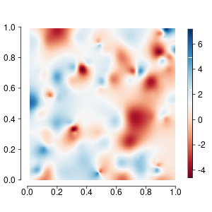
(a) raw $y(s)$

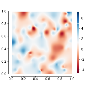
(b) raw $x(s)^{\mathrm{\scriptscriptstyle T}}\beta+z(s)$

(c) stacking of mean

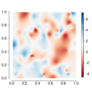
(d) stacking of predictive densities

(e) M0

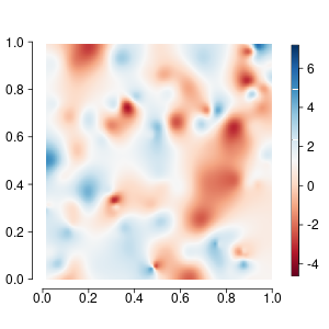
(f) MCMC

Figure 7: Interpolated maps of (a) the response $y(s)$, (b) the denoised response $x(s)\beta+z(s)$ and (c-f) the expected $y(s)$ on the $n_{h}=100$ held out locations generated by all competing algorithms for one data set in the first simulation.

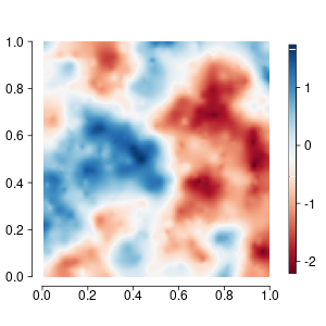
(a) raw

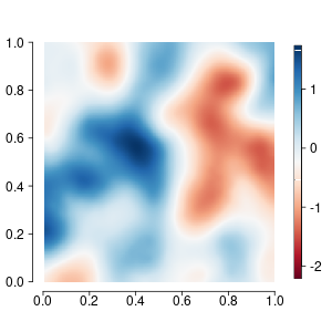
(b) stacking of mean

(c) stacking of predictive densities

(d) M0

(e) MCMC

Figure 8: Interpolated maps of (a) the latent process $z(s)$ and (b-g) the expected $z(s)$ on all $n=900$ sampled locations generated by all competing algorithms for one data set in the first simulation. The $n=900$ locations include both observed and unobserved locations

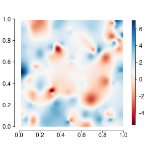
(a) raw $y(s)$

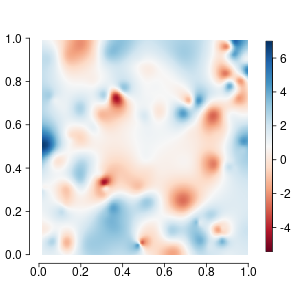
(b) raw $x(s)^{\mathrm{\scriptscriptstyle T}}\beta+z(s)$

(c) stacking of mean

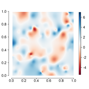
(d) stacking of predictive densities

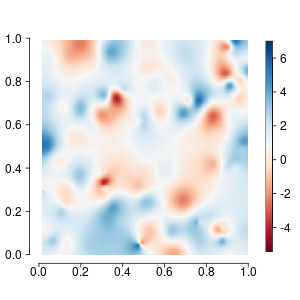
(e) M0

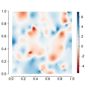
(f) MCMC

Figure 9: Interpolated maps of (a) the response $y(s)$, (b) the denoised response $x(s)\beta+z(s)$ and (c-f) the expected $y(s)$ on the $n_{h}=100$ held out locations generated by all competing algorithms for one data set in the second simulation.

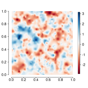
(a) raw

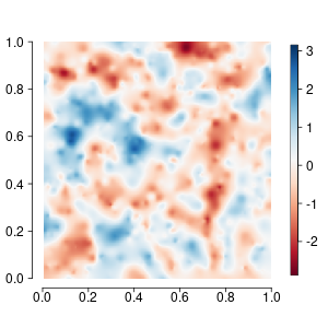
(b) stacking of mean

(c) stacking of predictive densities

(d) M0

(e) MCMC

Figure 10: Interpolated maps of (a) the latent process $z(s)$ and (b-g) the expected $z(s)$ on all $n=900$ sampled locations generated by all competing algorithms for one data set in the second simulation. The $n=900$ locations include both observed and unobserved locations

M.2 Distributions of the estimated $\nu$ and $\delta^{2}$

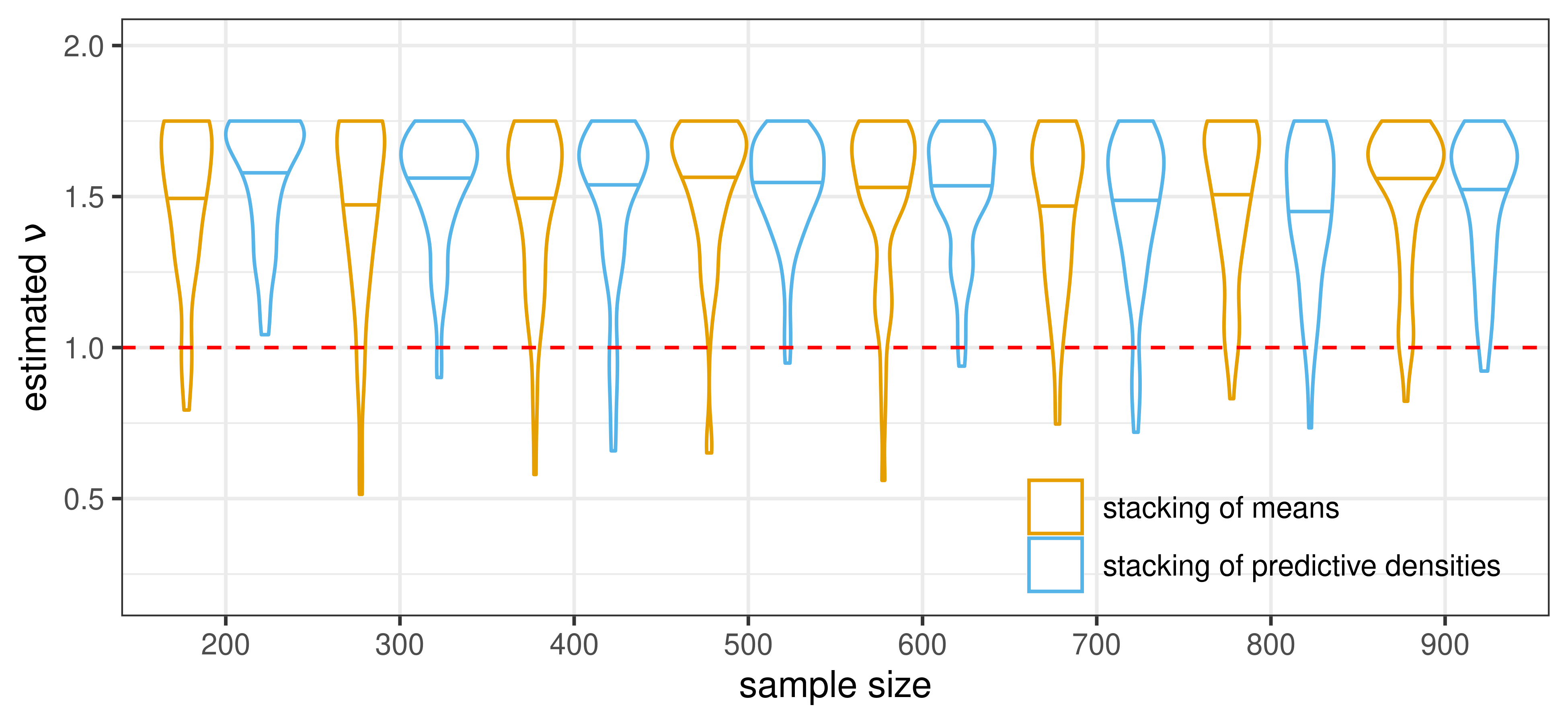
(a)

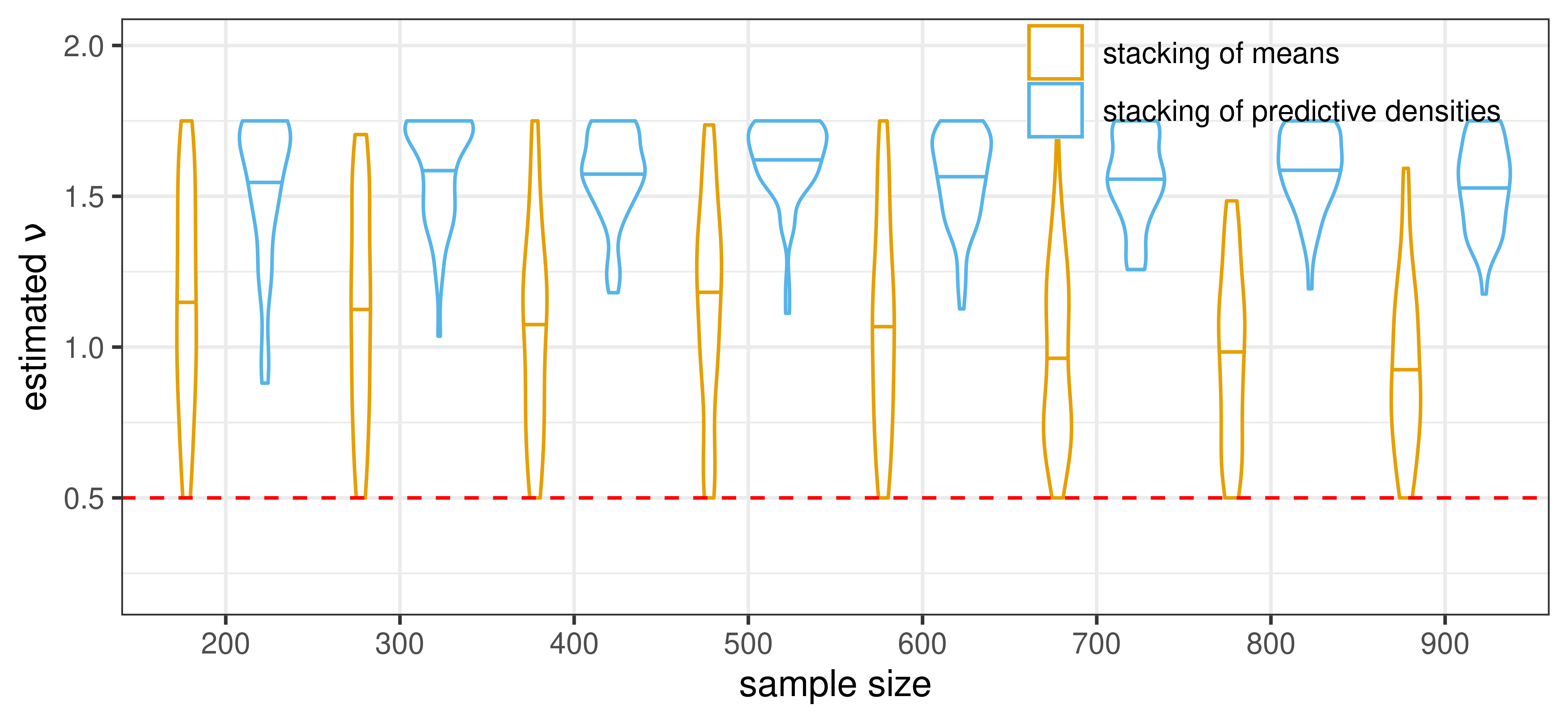
(b)

Figure 11: Distributions of the estimated $\nu$ in the first (a) and the second (b) simulation. The distribution of the counts are described through violin plots whose horizontal lines indicate the medians. The red dashed horizontal line indicates the actual value of $\nu$

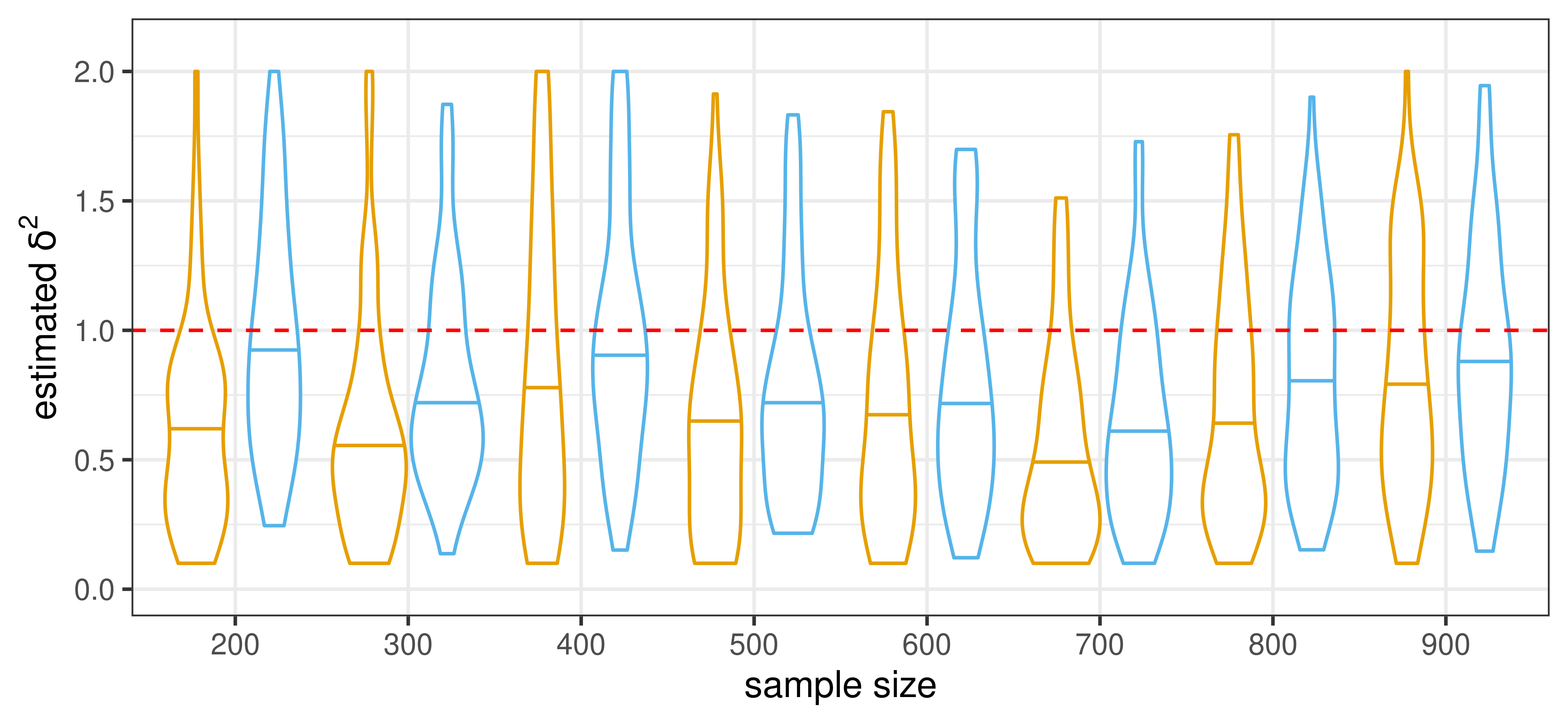
(a)

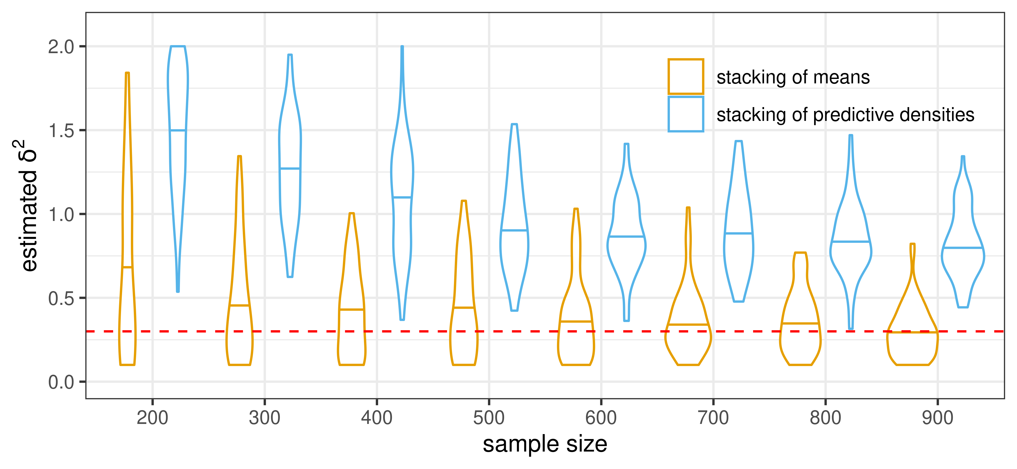
(b)

Figure 12: Distributions of the estimated $\delta^{2}$ in the first (a) and the second (b) simulation. The distribution of the counts are described through violin plots whose horizontal lines indicate the medians. The red dashed horizontal line indicates the actual value of $\delta^{2}$

Appendix N Compute the stacking weights for Stacking of means (in R code)

Let us format the expected outcome $\{y_{(\phi,\nu,\delta^{2})}^{(k)}\}^{k=1,\ldots,K}_{(\phi,\nu,\delta^{2})\in G_{all}}$ computed in Algorithm 1 by an $N\times G$ matrix $\hat{Y}$. Each column of $\hat{Y}$ stores the expected outcome $\{y_{(\phi,\nu,\delta^{2})}^{(k)}\}^{k=1,\ldots,K}$ for each candidate model, and it shares the same order of observed locations as the outcome $y$. Let $w=(w_{1},w_{2},\ldots,w_{G})^{\mathrm{\scriptscriptstyle T}}$ be the stacking weights, we need to find the weights that satisfy

$$\underset{w}{\mbox{argmin}}\{(y-\hat{Y}w)^{\mathrm{\scriptscriptstyle T}}(y-\hat{Y}w)\}\;,$$

under the constrain $\sum_{g}^{G}w_{g}=1$. Now we modify it into a quadratic programming (QP) problem.

$$(y- \hat{Y}w)^{\mathrm{\scriptscriptstyle T}}(y-\hat{Y}w)$$

$$=\{(y-\sum_{g}^{G}w_{g}\hat{Y}_{G})-\sum_{g}^{G-1}w_{g}(\hat{Y}_{g}-\hat{Y}_{G})\}^{\mathrm{\scriptscriptstyle T}}\{(y-\sum_{g}^{G}w_{g}\hat{Y}_{G})-\sum_{g}^{G-1}w_{g}(\hat{Y}_{g}-\hat{Y}_{G})\}$$

$$=(\tilde{y}-\tilde{Y}\tilde{w})^{\mathrm{\scriptscriptstyle T}}(\tilde{y}-\tilde{Y}\tilde{w})\;$$

where $\tilde{y}=y-\hat{Y}_{G}$, $\tilde{Y}=[(\hat{Y}_{1}-\hat{Y}_{G}):\cdots:(\hat{Y}_{G-1}-\hat{Y}_{G})]$, and $\tilde{w}=(w_{1},\ldots,w_{G-1})^{\mathrm{\scriptscriptstyle T}}$. And the QP problem has constrains $-\sum_{g=1}^{G-1}w_{g}\geq-1$ and $w_{g}\geq 0$ for $g=1,\ldots,G-1$.

References

- Abramowitz & Stegun (1965) Abramowitz, M. & Stegun, A. (1965). Handbook of Mathematical Functions: with Formulas, Graphs, and Mathematical Tables. Dover.
- Banerjee (2019) Banerjee, S. (2019). Geostatistics for environmental processes. In Handbook of Environmental and Ecological Statistics, A. E. Gelfand, M. Fuentes, J. A. Hoeting & R. L. Smith, eds. CRC press, Boca Raton, FL, pp. 81–96.
- Banerjee (2020) Banerjee, S. (2020). Modeling massive spatial datasets using a conjugate bayesian linear modeling framework. Spatial Statistics 37, 100417.
- Banerjee et al. (2014) Banerjee, S., Carlin, B. P. & Gelfand, A. E. (2014). Hierarchical Modeling and Analysis for Spatial Data. CRC Press, Boca Raton, FL.
- Berger et al. (2001) Berger, J. O., Oliveira, V. D. & Sansó, B. (2001). Objective bayesian analysis of spatially correlated data. Journal of the American Statistical Association 96, 1361–1374.
- Bernardo & Smith (1994) Bernardo, J. & Smith, A. (1994). Bayesian Theory. Chichester, UK: John Wiley and Sons.
- Bose et al. (2018) Bose, M., Hodges, J. S. & Banerjee, S. (2018). Toward a diagnostic toolkit for linear models with gaussian-process distributed random effects. Biometrics 74, 863–873.
- Bradley et al. (2020) Bradley, J. R., Holan, S. H. & Wikle, C. K. (2020). Bayesian hierarchical models with conjugate full-conditional distributions for dependent data from the natural exponential family. Journal of the American Statistical Association 115, 2037–2052.
- Breiman (1996a) Breiman, L. (1996a). Stacked regressions. Machine Learning 24, 49–64.
- Breiman (1996b) Breiman, L. (1996b). Stacked regressions. Machine learning 24, 49–64.
- Chilés & Delfiner (1999) Chilés, J. & Delfiner, P. (1999). Geostatistics: Modeling Spatial Uncertainty. John Wiley: New York.
- Clyde & Iversen (2013) Clyde, M. & Iversen, E. S. (2013). Bayesian model averaging in the m-open framework. Bayesian theory and applications 14, 483–498.
- Cressie (1993) Cressie, N. (1993). Statistics for Spatial Data. Wiley-Interscience, New York, revised ed.
- De Oliveira & Han (2022) De Oliveira, V. & Han, Z. (2022). On information about covariance parameters in gaussian matern random fields. Journal of Agricultural, Biological and Environmental Statistics 27, 690–712.
- Finley et al. (2019) Finley, A. O., Datta, A., Cook, B. C., Morton, D. C., Andersen, H. E. & Banerjee, S. (2019). Efficient algorithms for bayesian nearest neighbor gaussian processes. Journal of Computational and Graphical Statistics 28, 401–414.
- Gabry & Goodrich (2020) Gabry, J. & Goodrich, B. (2020). Prior distributions for rstanarm models. http://mc-stan.org/rstanarm/articles/priors.html.
- Handcock & Stein (1993) Handcock, M. S. & Stein, M. L. (1993). A bayesian analysis of kriging. Technometrics 35, 403–410.
- Hodges (2013) Hodges, J. S. (2013). Richly parameterized linear models: Additive, time series, and spatial models using random effects .
- Hoeting et al. (1999) Hoeting, J. A., Madigan, D., Raftery, A. E. & Volinsky, C. T. (1999). Bayesian model averaging: a tutorial (with comments by M. Clyde, David Draper and E. I. George, and a rejoinder by the authors. Statistical Science 14, 382 – 417.
- Kaufman & Shaby (2013) Kaufman, C. G. & Shaby, B. A. (2013). The role of the range parameter for estimation and prediction in geostatistics. Biometrika 100, 473–484.
- Le & Clarke (2017) Le, T. & Clarke, B. (2017). A bayes interpretation of stacking for m-complete and m-open settings. Bayesian Analysis 12, 807–829.
- Li et al. (2023) Li, C., Sun, S. & Zhu, Y. (2023). Fixed-domain posterior contraction rates for spatial gaussian process model with nugget. Journal of the American Statistical Association 0, 1–21.
- Madigan et al. (1996) Madigan, D., Raftery, A. E., Volinsky, C. & Hoeting, J. (1996). Bayesian model averaging. In Proceedings of the AAAI Workshop on Integrating Multiple Learned Models, Portland, OR.
- Murphy (2015) Murphy, K. P. (2015). Conjugate bayesian analysis of the gaussian distribution, 2007. URL https://www. cs. ubc. ca/~ murphyk/Papers/bayesGauss.pdf .
- Rasmussen & Williams (2006) Rasmussen, C. E. & Williams, C. K. I. (2006). Gaussian processes for machine learning. MIT Press, Cambridge, MA.
- Stein (1999) Stein, M. L. (1999). Interpolation of Spatial Data: Some Theory for Kriging. Springer-Verlag, New York.
- Tang et al. (2021) Tang, W., Zhang, L. & Banerjee, S. (2021). On identifiability and consistency of the nugget in Gaussian spatial process models. J. R. Stat. Soc. Ser. B. Stat. Methodol. 83, 1044–1070.
- Vehtari et al. (2016) Vehtari, A., Mononen, T., Tolvanen, V., Sivula, T. & Winther, O. (2016). Bayesian leave-one-out cross-validation approximations for gaussian latent variable models. The Journal of Machine Learning Research 17, 3581–3618.
- Wolpert (1992) Wolpert, D. H. (1992). Stacked generalization. Neural networks 5, 241–259.
- Yao et al. (2021) Yao, Y., Pir, G., Vehtari, A. & Gelman, A. (2021). Bayesian hierarchical stacking: Some models are (somewhere) useful. Bayesian Analysis 1, 1–29.
- Yao et al. (2020) Yao, Y., Vehtari, A. & Gelman, A. (2020). Stacking for non-mixing bayesian computations: The curse and blessing of multimodal posteriors. arXiv preprint arXiv:2006.12335 .
- Yao et al. (2018) Yao, Y., Vehtari, A., Simpson, D. & Gelman, A. (2018). Using stacking to average bayesian predictive distributions (with discussion). Bayesian Analysis 13, 917–1007.
- Zhang (2004) Zhang, H. (2004). Inconsistent estimation and asymptotically equal interpolations in model-based geostatistics. Journal of the American Statistical Association 99, 250–261.
- Zhang & Zimmerman (2005) Zhang, H. & Zimmerman, D. L. (2005). Towards reconciling two asymptotic frameworks in spatial statistics. Biometrika 92, 921–936.
- Zhang et al. (2021) Zhang, L., Banerjee, S. & Finley, A. O. (2021). High-dimensional multivariate geostatistics: A Bayesian matrix-normal approach. Environmetrics 32, e2675.
- Zimmerman & Stein (2010) Zimmerman, D. & Stein, M. (2010). Classical geostatistical methods. In Handbook of spatial statistics, A. E. Gelfand, P. Diggle, P. Guttorp & M. Fuentes, eds. CRC press, Boca Raton, FL, pp. 29–44.