AutoFocusFormer: Image Segmentation off the Grid

Abstract

Real world images often have highly imbalanced content density. Some areas are very uniform, e.g., large patches of blue sky, while other areas are scattered with many small objects. Yet, the commonly used successive grid downsampling strategy in convolutional deep networks treats all areas equally. Hence, small objects are represented in very few spatial locations, leading to worse results in tasks such as segmentation. Intuitively, retaining more pixels representing small objects during downsampling helps to preserve important information. To achieve this, we propose AutoFocusFormer (AFF), a local-attention transformer image recognition backbone, which performs adaptive downsampling by learning to retain the most important pixels for the task. Since adaptive downsampling generates a set of pixels irregularly distributed on the image plane, we abandon the classic grid structure. Instead, we develop a novel point-based local attention block, facilitated by a balanced clustering module and a learnable neighborhood merging module, which yields representations for our point-based versions of state-of-the-art segmentation heads. Experiments show that our AutoFocusFormer (AFF) improves significantly over baseline models of similar sizes.

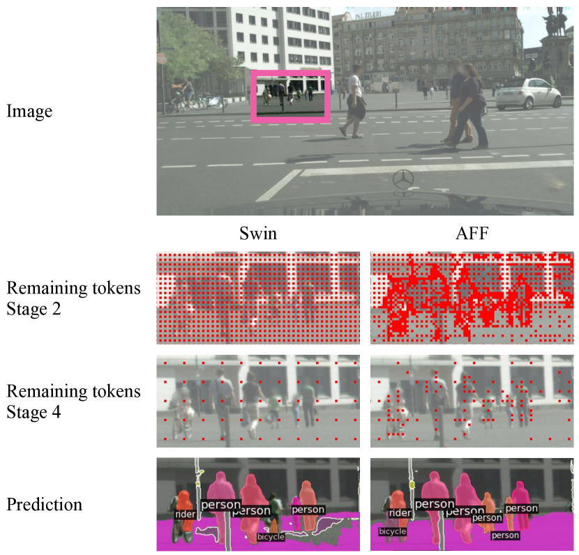
Figure 1: Comparison between on-grid model Swin [20] and off-grid model AFF. The red pixels indicate the locations of the remaining tokens. AFF downsamples non-uniformly, automatically focusing on more textured, important image regions, which lead to better performance on small objects in the scene.

1 Introduction

Typical real-world images distribute content unevenly. Consider the photo of a typical outdoor scene in Fig. 1: Large swaths of the image contain textureless regions like the ground, while a few regions contain many small objects. Despite this, most computer vision neural networks distribute computation evenly across the image; every pixel, regardless of texture or importance, is processed with the same computational cost. Popular convolutional neural networks operate on regularly-arranged square patches. Although recent transformer architectures do not strictly depend on a grid structure, many transformer-based methods adopt grid-based techniques such as stride-16 convolutions [5] and $7\times 7$ square windows for local attention [20].

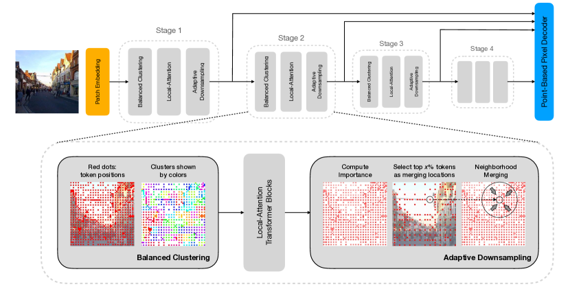
Figure 2: The network architecture of AutoFocusFormer. The model consists of four stages, each stage processing a successively downsampled set of tokens. Within each stage, tokens first go through balanced clustering, then attend to the tokens in their local neighborhoods defined by the nearby clusters in the following local-attention blocks, and finally adaptively merge into the set of downsampled output tokens with weights modulated by the learnable importance scores.

Despite its popularity, uniform downsampling is less effective for tasks that require pixel-level details such as segmentation. Here, uniform downsampling unfortunately makes tiny objects even tinier – possibly dropping needed, pixel-level information. To combat this, many techniques increase the input resolution [37, 7] to obtain better segmentation performance. This intuitively helps, as larger input will lead to higher resolution after downsampling. However, increasing input resolution is costly in memory and computation, as this brute-force bandaid neglects the underlying issue – namely, uniform downsampling. Some prior works amend this by irregularly sampling points in the segmentation decoder [17], but by still relying on a uniformly-downsampled convolutional encoder, these techniques remain susceptible to the pitfalls of uniform downsampling.

To address this concern, we need solutions that enable computer vision models to allocate computation non-uniformly across each image. In particular, we need a downsampling strategy that retains important details, while more aggressively summarizing texture-less regions such as sky or road. However, non-uniform downsampling breaks from the grid structure that existing architectures rely on. Prior work on adaptive downsampling [32, 18, 9] addresses this by simply using global attention, but global attention does not scale to resolutions much higher than that of ImageNet, such as those required for segmentation tasks.

To satisfy this need for adaptive, scalable downsampling strategies, we propose AutoFocusFormer (AFF). To our knowledge, AFF is the first end-to-end segmentation network with successive adaptive downsampling stages. To scale to higher resolutions required in segmentation tasks, AFF employs local attention blocks. In order to define local attention neighborhoods among irregularly sampled tokens, we develop a novel balanced clustering algorithm which employs space-filling curves to group irregular locations into neighborhoods. We also propose a novel adaptive downsampling module that learns the importance of different image locations through a differentiable neighborhood merging process (Fig. 4). Finally, we modify state-of-the-art segmentation heads so that they can be applied on the irregular-spaced representations our backbone generates.

Our AutoFocusFormer attains state-of-the-art performance with less computational cost across major segmentation tasks, with especially strong results when using smaller models. Furthermore, by moving away from the grid structure, our downsampling strategy can support a larger range of computational budget by retaining any number of tokens, rather than operating only at rates of $1/4$, $1/16$ etc.

To summarize, our contributions are:

• To our knowledge, we introduce the first end-to-end segmentation network with successive adaptive downsampling stages and with flexible downsampling rates.

• To facilitate a local attention transformer on irregularly spaced tokens, we propose a novel balanced clustering algorithm to group tokens into neighborhoods. We also propose a neighborhood merging module that enables end-to-end learning of adaptive downsampling.

• We adapt state-of-the-art decoders such as deformable DETR [55], Mask2Former [2] and HCFormer [40] to operate on irregularly spaced sets of tokens.

• Results show that our approach achieves state-of-the-art for both image classification and segmentation with fewer FLOPs, and improves significantly on the recognition of small objects in instance segmentation tasks.

2 Related Work

Transformer backbones for Vision. The seminal Vision Transformer (ViT) [5] demonstrated that simple image patch encodings combined with self-attention enable impressive modeling capacity on image classification tasks. However, ViTs lack hierarchical feature maps which are critical for dense prediction tasks. Various improvements have since been proposed, e.g., MViT and PVT [8, 43] propose using feature hierarchies similar to those of standard convolutional networks. However, they still operate on global attention, which suffers from quadratic complexity w.r.t. the input size, hence struggling with high resolution inputs. One solution is to apply attention only on the low resolution feature maps, as in BoT [39] and LeViT [11]. Other approaches modify the attention operation. SegFormer[46] computes attention in earlier layers on a concatenation of many tokens. PoolFormer and AFT[49, 51] replace attention with pooling based operations which reduces the quadratic complexity to linear. Swin Transformer and SASA [20, 31] replace the global attention with local attention, where attention is computed only in a small local window, which achieves better efficiency.

Clustering-based Attention. Clustering based sparse attention has been proposed in language and vision [35, 41, 53, 42]. However, these works do not involve adaptive downsampling which is central to our method. Most works attempt to cluster learned features, whereas we cluster based on token locations. We have also studied clustering of features, but found it not to provide significant improvements, while adding significant complexity to the model. Clustering ideas have also been applied in decoders [48, 40] which differs from our work as we apply clustering in the encoder.

Adaptive downsampling. There have been many attempts to combine adaptive downsampling with vision Transformers, such as AdaViT [25], DynamicViT [32], A-ViT [47], etc. Dynamic Grained Encoder[38] proposes to learn different grid downsampling rates for different regions. EViT[18] proposes to merge the “uninformative” patches into one. PS-ViT [50] proposes to learn offsets to the original grid patch locations. However, all of these solutions are still based on global attention. Most of them do not prune away “uninformative” patches during training, either due to the need for gradients to flow through those patches [32] or the need for uniform size across the batch [47]. Hence, they cannot scale to high-resolution segmentation tasks, but only focus on speeding up ImageNet classification.

How to make the adaptive downsampling module learnable has itself been a significant challenge. Some methods turn to heuristics such as the attention values [9]; some turn to policy gradient [27]; some turn to the Gumbel-Softmax trick [23] to obtain a differentiable binary mask [25, 32]. To directly obtain gradients from the task loss, merging tokens [36, 18] seems to be a more natural strategy than deleting tokens. We develop a novel neighborhood merging module, adaptively choosing the merging locations, providing gradients directly from the task loss to the “importance scores” of the tokens. To our best knowledge, our work is the first end-to-end framework with local attention blocks that uses adaptive downsampling in multiple stages, and is scalable to high-resolution segmentation tasks.

Point cloud networks. Prior works that directly operate on a set of irregular points are mostly designed for 3D point clouds, such as PointNet++ [30], PointConv [45] and Point Transformer [52]. They often choose $k$-nearest-neighbors or an $\epsilon$-ball to find the neighborhood for each point. We make limited usage of PointConv in our decoder model to replace $3\times 3$ convolution.

3 Method

Our goal is to perform adaptive downsampling instead of the traditional grid-based downsampling. Specifically, we want to retain more 2D image locations in “informative” areas (e.g., areas which depict cluttered small objects), and more succinctly summarize “unimportant” areas (e.g., a purely blue sky). Because the chosen locations have uneven density, our model treats the locations as a set of irregularly-spaced tokens rather than a rectangular grid.

As we mentioned earlier, global-attention transformers are computationally demanding for segmentation tasks. Thus, local transformer models are a natural choice for our goal due to their computation efficiency on larger images. However, the regular grid local window mechanism in methods like Swin Transformer [20] is not amenable to adaptive irregular downsampling, so we propose to cluster pixels and perform attention on clusters.

Specifically, our backbone model (Fig. 2) starts with a patch embedding module (2 layers of $3\times 3$ convolution with stride 2), and then continues with several stages. Each stage consists of: 1) a clustering algorithm (Section 3.1); 2) several local-attention transformer blocks (Section 3.2); 3) the novel adaptive downsampling module (Section 3.3). Finally, task-specific heads are attached to the backbone for different tasks such as image classification, semantic and instance segmentation.

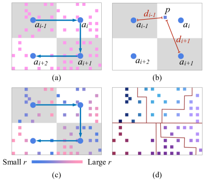
Figure 3: Illustration of the balanced clustering algorithm. (a) Tokens are quantized to space-filling anchors. A space-filling curve orders the anchors ($a_{i-1},a_{i},\cdots$). (b) For each token (e.g., token $p$ quantized to $a_{i}$), calculate the ratio of its distance to the “previous” and the “next” anchor ($r(p)=d_{i-1}(p)/d_{i+1}(p)$). (c) Order tokens quantized to the same anchor in ascending order of $r$. (d) Sort all tokens based on the anchor order and the local token order. Partition the sorted tokens into equal-sized clusters.

3.1 Clusters and Neighborhoods

A local neighborhood on a 2D grid can be conveniently defined by slicing out a square window. In contrast, for an unordered set of points, the conventional approach to identify neighbors in a 3D point cloud [30, 45] relies on algorithms such as $k$-nearest-neighbors (kNN), which compute pairwise distances between points.

A naive kNN algorithm has a quadratic time complexity. Interestingly, many of the algorithms to speed up kNN (e.g., [15]) involve a first step of $k$-means clustering on given points so as to reduce the search space for the neighbors. Inspired by this approach, we also use clusters in defining local neighborhoods, i.e., we divide the tokens into clusters, and define neighborhoods as entailing several nearby clusters. Unfortunately, traditional clustering algorithms such as $k$-means or locality-sensitive hashing do not directly fit our purpose. First, they require multiple iterations or rounds of hashing and are thus slow, compared to a forward pass in a deep net. More importantly, they result in clusters with different numbers of assigned points. Unevenly sized clusters results in tensors padded with zeros, which leads to wasted memory and time.

Noting that we are only clustering on 2D positions but not higher dimensions, we propose to address the aforementioned concerns with a novel balanced clustering method.

3.1.1 Balanced Clustering

Instead of conventional iterative approaches, our method to obtain a perfectly balanced clustering is to arrange 2D locations on the image into a 1D array, and then partition the array into groups of equal size. For this we consider space-filling curves [29], which arrange 2D locations on a 1D line while attempting to preserve the 2D distance measure [26]. Hence, points that are close on the line are also reasonably close in the 2D space. However, due to the conversion from 2D to 1D, it is impossible to completely preserve the 2D metric, and artifacts occur if we directly utilize space-filling curves to partition tokens into clusters. To partially alleviate this concern, we adopt a 2-stage process for the clustering. The idea is to utilize space-filling curves only at a coarse level to obtain an ordering for sparsely and regularly sampled 2D image locations. Then, tokens are ordered based on the 2D distances to these locations.

Concretely, we first divide the image into a coarse regular grid with the number of square patches being similar to the intended number of clusters. We refer to the center of each square patch in the grid as a space-filling anchor. A space-filling curve establishes an ordering among the anchors. Given this ordering, for a token with position $p\in\mathbb{R}^{2}$ belonging the anchor $a_{i}\in\mathbb{R}^{2}$, we can define its previous anchor $a_{i-1}$ and next anchor $a_{i+1}$. Then, we calculate the ratio $r$ of distances from token $p$ to the two anchors via

$$r(p)=\dfrac{d_{i-1}(p)}{d_{i+1}(p)}=\dfrac{\|p-a_{i-1}\|_{2}}{\|p-a_{i+1}\|_{2}}$$ (1)

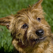
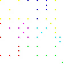
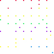
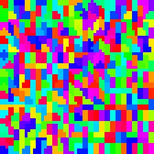
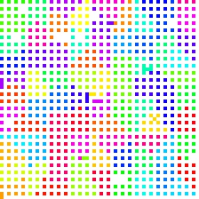
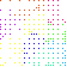
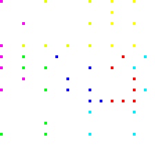
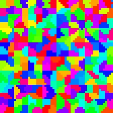
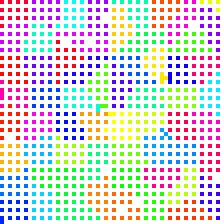
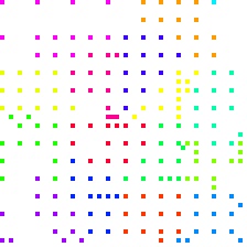
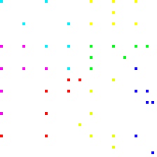
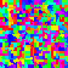
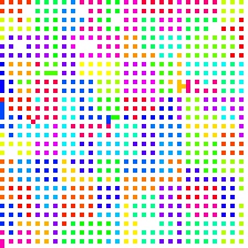
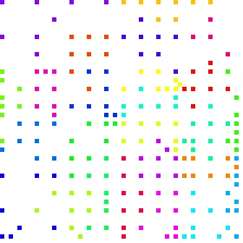
Figure 5: Visualization of the balanced clustering results with different configurations of anchors and space-filling curves. For the cases without anchors, the space-filling curve is applied directly on the tokens. From the results, we observe the use of anchors to be critical for obtaining more rounded and separated clusters. Although Peano and Hilbert are recursive curves, the uneven density of the tokens due to adaptive sampling still breaks the local euclidean metric if we directly apply these curves on the tokens.

for all tokens $p$. Now, within each square patch, we order the tokens in ascending order of $r$, so that tokens closer to the previous anchor are placed earlier. This procedure hence establishes an ordering of all the tokens. Finally, to obtain balanced clustering we simply partition the array into groups of equal size. Fig. 5 illustrates the entire algorithm.

Because we can find the corresponding space-filling anchor for each token in $O(1)$ time by simply quantizing their coordinates, the overall time complexity of the clustering is no more than sorting all the token locations in their local patches once, which is negligible compared to the network time complexity because feature channels are not involved. Note that the clustering algorithm only needs to be performed once at the beginning of each stage, and the cluster information can be used for all attention blocks in the stage, as well as the downsampling module at the end.

Different from prior balanced clustering work [1], this algorithm is not iterative and results in perfectly balanced clusters. It also guarantees that each token belongs to a single cluster, different from RoutingTransformer [35], where some tokens may not belong to any cluster. However, note that our balanced clustering is only suitable for low-dimensional points. In early stages of this research, we explored clustering with embedded features instead of just 2D locations, but the performance difference was negligible. Hence, we decided to cluster on the locations only, which allowed us to utilize the proposed algorithm to generate perfectly balanced clusters. Please see the supplementary material for experiments validating our clustering approach.

3.1.2 Neighborhoods from clusters

In order to encourage information flow across the whole image, it is important that attention is not limited to only locations within the same cluster. E.g., in Swin Transformers [20], shifting windows between consecutive layers allows pixels to attend to different neighbors in different layers. However, in our case, re-clustering every layer would add undesired computation. Hence, we opt to use smaller clusters and allow each token to attend to tokens from $R$ nearby clusters. To achieve this, we use a neighborhood size several times larger than the cluster size. This is beneficial because the neighborhoods are overlapping, guaranteeing information exchange between the clusters.

3.2 Transformer Attention Blocks

At any stage, let $N$ be the number of tokens, $M$ be the number of neighbors for each token, $H$ be the number of heads, and $C$ be the number of feature channels. The local attention $A$ of one single head with relative position embedding is computed by having each token attend to all the other tokens in its neighborhood via

$$A=\text{softmax}(QK^{T}+P),$$ (2)

where $Q\in\mathbb{R}^{N\times C/H},K\in\mathbb{R}^{M\times C/H},A\in\mathbb{R}^{N\times M},P\in\mathbb{R}^{N\times M}$ are query, key, attention and position embedding matrices with

$$P_{i,j}=w(p_{i}-p_{j}).$$ (3)

Here, $p_{i},p_{j}$ are the $(x,y)$ coordinates of two neighboring tokens, and $w(\cdot)$ is a function that returns a scalar position embedding for this head. For models with fixed-shape neighborhoods, the relative position embeddings can be stored in a matrix and read when needed. But for our model, the positions of the neighbors are unknown beforehand, and thus we need to project the difference of the coordinates to a position embedding via a learnable function. We implement $w$ as one fully-connected layer.

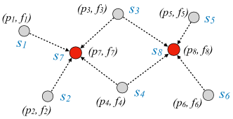
Figure 4: Illustration of the adaptive downsampling module. First, importance scores $s_{i}$ are calculated from the token features $f_{i}$. Then, tokens with the highest scores are selected as merging centers (e.g., $p_{7}$ and $p_{8}$). Finally, neighborhoods are merged with weights modulated by the importance scores $s_{i}$.

3.3 Adaptive downsampling

At the end of each but the final stage, we employ a downsampling module. The downsampling module includes two components, a learnable scoring component for choosing the most important tokens, and the neighborhood merging step to merge the neighbors around selected tokens.

3.3.1 Learnable Importance Score

We learn to predict a scalar score $s_{i}$ for the $i$-th token to indicate its importance w.r.t. the task loss. A main difficulty in learning this score is that downsampling limits the number of selected tokens. If the task loss is only backpropagated to the selected tokens, tokens that were not selected might not receive any gradient. In order to backpropagate gradients to all the tokens, we propose to learn the importance score for each token in conjunction with the neighborhood merging process.

To illustrate this, assume we are merging a neighborhood around a particular token at location $p_{c}$. Similar to attention blocks, a neighborhood $\mathcal{N}(p_{c})$ is obtained from its nearest $R$ clusters and the $i$-th neighboring token is denoted as a tuple $(p_{i},f_{i})$ with location $p_{i}=(x_{i},y_{i})$ and features $f_{i}\in\mathbb{R}^{C}$. In the neighborhood, merging is performed using a modification of a PointConv layer[45] as follows:

$$f_{\text{merged}}(p_{c})\!=\!\text{vec}\left(\!\sum_{(p_{i},f_{i})\in\mathcal{N}(p_{\text{c}})}\overbrace{\sigma(l(f_{i}))}^{\text{$s_{i}$}}\cdot\mathbf{W}(p_{i}-p_{\text{c}})f_{i}^{\top}\right)U,$$ (4)

where $f_{\text{merged}}\in\mathbb{R}^{C^{\prime}}$ is the merged output with $C^{\prime}$ outputs, $\text{vec}(\cdot)$ means vectorization, $\sigma(\cdot)$ is the sigmoid function, $l(\cdot)$ is a fully-connected layer predicting the scalar “importance score”, $\mathbf{W}(\cdot)$ is a multi-layer perceptron (MLP) with output shape $C_{\text{mid}}\times 1$, which creates different weighted combinations of the input features $f_{i}$ in the neighborhood. The weights are learned to be a function of the relative coordinates between the location of each neighboring token and the merging center location $p_{c}$. Finally, $U\in\mathbb{R}^{C_{\text{mid}}C\times C^{\prime}}$ is implemented as a fully-connected layer.

Note, Eq. (4) is similar to PointConv $f=\mathrm{vec}(\sum\mathbf{W}f^{\top})U$, which was shown to be equivalent to one continuous convolution layer [45]. We add $s_{i}=\sigma(l(f_{i}))$ to modulate this function, which allows the model to “turn off” the unimportant tokens during neighborhood merging, keeping their features from being utilized in the next stage. Thus, the score $s_{i}$ can be viewed as an indicator, denoting how important the model thinks a token is. This score can henceforth be used to select the merging centers.

This formulation allows us to directly learn the score $s_{i}$ from the task loss without resorting to costly techniques such as a policy gradient used in prior work [27]. Some previous works use Gumbel Softmax/Sigmoid [25] to obtain a differentiable binary mask, in order to keeping gradients flowing to the “deleted” tokens after downsampling; since we adopt the merging strategy rather than deletion, we do not need such a hard binary mask. We provide visualizations of the neighborhood merging process in Fig. 4.

3.3.2 Grid priors and Selection of Tokens to Sample

The final score used for selecting tokens as merging centers is $g_{i}+\alpha s_{i}$, a weighted sum between the learned score $s_{i}$ and a grid prior $g_{i}$, with a hyperparameter $\alpha$. While $s_{i}$ is only based on the feature vector, the grid prior helps the model to differentiate between similar tokens at different locations, thus facilitating the model to perform proper, uniform-stride downsampling in local texture-less regions. Our grid prior $g_{i}$ mimics the behavior of the traditional grid downsampling – alternatingly assigning 1 and 0 to the tokens. However, in stages where the tokens are already irregularly sampled, adding a regular grid prior is no longer reasonable. Hence, we advocate for an “adaptive” grid prior that takes the local density of the sampled tokens into account.

Specifically, the adaptive prior chooses a local grid level based on the local stride of the sampled tokens. For each token $p_{i}=(x_{i},y_{i})$, we assign its “stride” $t_{i}=2^{\lceil\log_{2}\min_{j}\|p_{i}-p_{j}\|_{1}\rceil}$ to be the distance from the token to its nearest neighbor, rounded up to the nearest power of 2. For example, if the token is $3$ pixels apart from its nearest neighbor, it is assigned stride $t_{i}=4$. Then, we assign $g_{i}=1$ if $(x_{i}\mod 2t_{i}=0)\wedge(y_{i}\mod 2t_{i}=0)$. That is, we want to downsample the local stride from $t_{i}$ to $2t_{i}$. Hence, if $t_{i}=1$, then $g_{i}=1$ on alternating pixels, and if $t_{i}=2$, then $g_{i}=1$ every 4 pixels. Furthermore, we set the grid prior to infinity for tokens with ($x_{i}\mod 2^{j+1}=0)\wedge(y_{i}\mod 2^{j+1}=0)$ in the $j$-th stage. We call these tokens “reserved”. We reserve these coarse-grid tokens to ensure the connectivity among remote regions in the image throughout the forward pass.

In summary, the workflow of adaptive downsampling is as follows: 1) obtain importance score $s_{i}=\sigma(l(f_{i}))$ for each token $f_{i}$, 2) calculate the grid prior $g_{i}$ for each token, 3) pick the top-$x$% (e.g., 1/4 or 1/5) tokens with highest $g_{i}+\alpha s_{i}$ values; 4) perform neighborhood merging around the location of the top-$x$% tokens using the formulation given in Eq. (4) and obtain the merged tokens for the next stage.

4 Implementation Details

4.1 Point-based versions of segmentation heads

Traditional segmentation heads only operate on a set of rectangular hierarchical feature maps. In our case, the output of the backbone is a set of features on irregularly spaced tokens. To compare with prior work, we convert two recent Transformer-based segmentation heads, Mask2Former and HCFormer, so as to operate on irregularly spaced tokens.

Mask2Former [2] uses the multi-scale deformable attention from deformable DETR [55] as part of its pixel decoder. In the multi-scale deformable attention layer, a token in one feature map attends to $k$ locations in every hierarchical level. It learns the offset $\Delta p_{i}$ between its own location $p_{c}$ and the $i$-th sampling location $p_{i}=p_{c}+\Delta p_{i}$ by performing bilinear interpolation on the $2\times 2$ patch surrounding $p_{i}$. We replace the bilinear interpolation with an inverse distance weighting-based interpolation, with a learnable power initialized at 6. Specifically, we gather 4 tokens closest in Euclidean space to $p_{c}+\Delta p_{i}$, and use the inverse of their distances to $p_{c}+\Delta p_{i}$ raised to the learned power for a weighted average of their features (weights sum normalized to 1), to obtain the feature of the sampled neighbor. In addition, we replace the $3\times 3$ convolutions in the pixel decoder by a PointConv layer. We implement the weight net $w(\cdot)$ in all the PointConv layers used in our model (including those in adaptive downsampling) as one fully-connected layer followed by one LayerNorm and one GELU activation. The mid-channel number $C_{\text{mid}}$ is set to 4.

We introduce the other segmentation head HCFormer [40] in the supplementary material.

4.2 Scale and Rotation Invariance

Our adaptive downsampling mechanism allows us to utilize the same number of features for both small and large scale objects. However, this creates a difficulty for the position embedding to achieve scale invariance, since tokens on a smaller object are closer together and have smaller relative distances, resulting in vastly different position embedding values than tokens on a large object.

To address this concern, we expand the relative position vector from $(\Delta x,\Delta y)=(x_{i}-x_{j},y_{i}-y_{j})$ to

$$\!\left(\!\Delta x,\Delta y,\sqrt{\Delta x^{2}\!+\!\Delta y^{2}},\dfrac{\Delta x}{\sqrt{\Delta x^{2}\!+\!\Delta y^{2}}},\dfrac{\Delta y}{\sqrt{\Delta x^{2}\!+\!\Delta y^{2}}}\!\right)\!.$$ (5)

Note, the latter three terms are distance, cosine and sine values of the relative position. Distance is rotation-invariant and the angle values are scale-invariant. These expanded terms facilitate learning appropriate scale-invariant and rotational-invariant embeddings.

4.3 Blank Tokens

During early experiments on ImageNet, we observed abnormally large feature norms for tokens in texture-less corners of the images, usually far away from any object, both for our model and for Swin [20] Transformers. We suspect this is because of the strong gradient softmax has when it cannot separate near-identical (yet irrelevant) features. To eliminate this artifact, we introduced a learnable blank token $(K_{\text{blank}}^{ij},V_{\text{blank}}^{ij})\in\mathbb{R}^{C}\times\mathbb{R}^{C}$ shared by all neighborhoods in the $j$-th transformer block in the $i$-th stage. Thus, when there is no useful content in the neighborhood, the softmax operator can learn to simply attend to the blank token and avoid attempting to distribute attention in textureless regions.

Variant	# Blocks	Dim	Heads	MLP Ratio	Cluster Size	Neighborhood Size	# Params	FLOPs
AFF-Mini	2,2,6,2	32,128,256,384	2,4,8,16	2	8	48	6.75M	1.08G
AFF-Tiny	3,4,18,5	64,128,256,512	2,4,8,16	3	8	48	27.02M	4.03G
AFF-Small	3,4,18,2	96,192,384,768	3,6,12,24	3	8	48	42.61M	8.16G
AFF-Base	3,4,18,2	128,256,512,1024	4,8,16,32	3	24	144	75.34M	42.54G

Table 1: Configurations of AFF.

	Model	Top-1 Acc	# Params	FLOPs
Mini	A-ViT-T+distl. [47]	72.4%	5M	0.8G
	Token Pooling DeiT-e318 Sparsity level 5 [24]	76.8%	-	1.1G
	Swin-Mini‡	76.9%	6.76M	1.07G
	EdgeViT-XS [28]	77.5%	6.7M	1.1G
2-5	AFF-Mini	78.2%	6.75M	1.08G
	AFF-Mini-1/5	77.5%	6.75M	0.72G
Tiny	DynamicViT-DeiT-S/0.7 [32]	79.3%	-	2.9G
	TokenLearner S/32(22) [36]	79.4%	-	3.3G
	A-ViT-S+distl. [47]	80.7%	22M	3.6G
	AdaViT [25]	81.1%	-	3.9G
	PS-ViT-B/14 [50]	81.7%	21.3M	5.4G
	LightViT-B [14]	82.1%	35.2M	3.9G
	PVT v2-B2 [44]	82%	25.4M	4G
	Swin-Tiny	81.3%	28M	4.5G
	Swin-Tiny‡	81.9%	27M	4G
	ConvNeXt-Tiny [21]	82.1%	28M	4.5G
2-5	AFF-Tiny	83%	27M	4G
	AFF-Tiny-1/5	82.4%	27M	2.74G
Small	Swin-Small	83%	50M	8.7G
	Swin-Small‡	82.9%	42.6M	8.14G
	ConvNeXt-Small [21]	83.1%	50M	8.7G
	PS-ViT-B/18 [50]	82.3%	21.3M	8.8G
	TokenLearner B/32(20) [36]	82.7%	-	11.5G
2-5	AFF-Small	83.5%	42.6M	8.16G
	AFF-Small-1/5	83.4%	42.6M	5.69G
Base	Swin-Base†	86.4%	88M	47.0G
	AFF-Base†	86.2%	75.3M	42.5G

Table 2: ImageNet Top-1 validation accuracy comparison at $224\times 224$ resolution. “1/5” means the model uses 1/5 downsampling rate instead of the traditional 1/4 downsampling rate. “-” means not reported. The Swin backbones^‡ are trained using the same architecture configuration and training settings as our model. The base models^† are pre-trained on ImageNet-22K and subsequently fine-tuned on ImageNet-1K at $384\times 384$ resolution.

5 Experiments

5.1 Image Classification on ImageNet-1K

We evaluate on image classification using ImageNet-1K [4], which contains 1.28M training images and 50K validation images from 1000 classes.

Settings. Table 1 contains specifications for the different model sizes used in our comparisons. Unless stated otherwise, we use the “1/4” downsampling rate, cluster size 8 and neighborhood size 48 (i.e., we collect neighbors from the nearest 6 clusters for each token). For ImageNet only, we switch to global attention in the last stage, because at an input resolution of $224\times 224$, the last stage only has 49 tokens left. We set the hyperparameter $\alpha=4$ in the merging center score calculation. We largely follow the training hyperparameters from Swin Transformers. We train for 300 epochs.

Results. We present results in Table 2, divided into sections according to model sizes. Compared to Swin [20], we obtain +1.3%, +1.7% and +0.5% improvement for Mini, Tiny and Small, respectively. For a fair comparison, we trained Swin-Tiny and Swin-Small using our own architecture configuration, training settings and patch embedding layer, and we still obtain +1.1% and +0.6% improvement, respectively. The difference is not large, which is expected because adaptive downsampling is mainly geared toward dense prediction tasks. We did outperform all previous adapative downsampling approaches with global attention such as AdaViT, DynamicViT and A-ViT.

We further demonstrate our model’s capability to use flexible downsampling rates by showing the results with a 1/5 downsampling rate. Across all sizes, the 1/5 downsampling rate brings more than 30% drop in FLOP count compared to the 1/4 downsampling counterparts, with minimal accuracy drop and still beating all Swin baselines.

5.2 Segmentation

Datasets. We evaluate on semantic, instance, and panoptic segmentation using 3 datasets: ADE-20K [54] is a semantic segmentation dataset containing 150 categories across 20K training images and 2K validation images. Cityscapes [3] is a street-view dataset with high quality annotations, containing 2975 training images and 500 validation images, with a total of 19 object classes. COCO 2017 [19] is an instance segmentation dataset, containing 118K training and 5K validation images.

Settings. We mostly follow the settings of Mask2Former [2]. Please see the supplementary for details. Tasks with Swin-Mini backbone are trained under the same settings as AFF-Mini. Other Swin Transformer results are taken from [2].

Results. We present the results of semantic segmentation on ADE20K [54] (Table 3), instance and panoptic segmentation on Cityscapes [3] (Table 4) and instance segmentation on COCO [19] (in supplementary).

For semantic segmentation on ADE20K (Table 3), we show mIoU improvement across all three sizes compared to the Swin baselines: +2.4% for Mini, +1.9% for Mini-1/5; +2.5% for Tiny, +2.3% for Tiny-1/5; and +0.6% for Small-1/5. Our 1/5 downsampling-rate models decrease FLOP count by 20%, while improving over Swin across model sizes. We furthermore isolate the effect of changing the Mask2Former head to operate on point clouds (Section 4.1). Using Swin-Mini on semantic segmentation, we find the modified head reduces FLOP count (-9.4%) with slightly lower performance (-0.4%).

For instance and panoptic segmentation on Cityscapes (Table 4), both our Tiny and Small models demonstrate a solid improvement over the baselines with the Swin backbone. For Tiny, our model improves the Panoptic PQ metric by +1.8%, and the Instance AP by +3.0%. For Small, our model improves the Panoptic PQ metric by +2.1%, and the Instance AP by +2.2%. Note that the overall performance of AFF-Tiny is on par with Swin-Base, a model 3.3x larger; AFF-Small is on par with Swin-Large, a model 4.6x larger, while both baselines are pre-trained with $\mathbf{10}$ times more data on ImageNet22k [33].

Backbone	Segmentation Head	Crop Size	mIoU	FLOPs
Swin-Mini‡	Mask2Former [2]	512	44.5	54G
Swin-Mini‡	Mask2Former* [2]	512	44.1	48.9G
AFF-Mini	Mask2Former* [2]	512	46.5	48.3G
AFF-Mini-1/5	Mask2Former* [2]	512	46.0	39.9G
MiT-B2	SegFormer [46]	512	46.5	62.4G
PVT v2-B3 [44]	Semantic FPN [16]	512	47.3	62.4G
Swin-Tiny	Mask2Former [2]	512	47.7	74G
AFF-Tiny	Mask2Former* [2]	512	50.2	64.6G
AFF-Tiny-1/5	Mask2Former* [2]	512	50.0	51.1G
PVT v2-B5 [44]	Semantic FPN [16]	512	48.7	91.9G
MiT-B5	SegFormer [46]	640	51	183.3G
Swin-Small	Mask2Former [2]	512	51.3	98G
AFF-Small	Mask2Former* [2]	512	51.2	87G
AFF-Small-1/5	Mask2Former* [2]	512	51.9	67.2G

Table 3: Semantic segmentation on ADE20K val. “1/5”: backbone uses 1/5 downsampling rate instead of 1/4. * : Segmentation head modified to accept point cloud input. The Swin backbone^‡ is trained using the same architecture configuration and training settings as our model. Seed fixed at 0.

Backbone	Segmentation Head	Panoptic PQ (s.s.)	Instance AP	Backbone # Params
AFF-Mini	Mask2Former* [2]	62.7	40.0	6.75M
Swin-Tiny	Mask2Former [2]	63.9	39.7	28M
AFF-Tiny	Mask2Former* [2]	65.7	42.7	27M
Swin-Small	Mask2Former [2]	64.8	41.8	50M
AFF-Small	Mask2Former* [2]	66.9	44.0	42.6M
Swin-Base†	Mask2Former [2]	66.1	42	88M
AFF-Base†	Mask2Former* [2]	67.7	46.2	75.3M
Swin-Large†	Mask2Former [2]	66.6	43.7	197M

Table 4: Segmentation on Cityscapes. We set $\alpha=8$. * The segmentation head is modified to accept point cloud input. ^† Backbone pre-trained with ImageNet-22K. Seed fixed at 0.

5.3 Ablations

In Table 5, we ablate design choices using AFF-Mini. For example, replacing our adaptive downsampling with the downsampling approach in Swin[20] reduces top-1 ImageNet accuracy by 0.5%. Replacing our expanded position embedding with a baseline position embedding – passing only $(x,y)$ differences as input to the position embedding function – reduces top-1 ImageNet accuracy by 0.9%.

Variant	Downsampling rate	ImageNet1K Top-1 Acc
Full model	1/5	77.5%
Remove grid prior	1/5	76.6%
Remove expanded relative position	1/5	76.6%
Remove blank token	1/5	76.9%
Remove reserved tokens	1/5	77.2%
Full model	1/4	78.2%
Use PatchMerging from Swin [20]	1/4	77.7%

Table 5: Ablation studies based on AFF-Mini.

In Table 6, we present how the hyperparameter $\alpha$ influences the Top-1 accuracy on ImageNet and instance segmentation AP on Cityscapes [3]. $\alpha$ is used to balance the weight between the grid prior $g_{i}$ and the importance score $s_{i}$. The larger the $\alpha$ is, the more “adaptive” the remaining tokens are. For ImageNet classification, a larger $\alpha$ results in minor degradation in performance, while a reasonably large $\alpha$ results in better performance for instance segmentation. This is expected, as our adaptive downsampling module allocates more tokens to smaller objects and details around object boundaries. While this might not be needed by the usually centered objects in ImageNet, it is particularly beneficial for instance segmentation.

$\alpha$	ImageNet-1K Acc	Cityscapes Instance AP
2	78.4%	37.5
4	78.2%	38.7
6	-	38.7
8	-	40.0
10	-	37.8
12	-	38.1

Table 6: Ablation studies on $\alpha$ using AFF-Mini and Mask2Former [2] heads. Larger $\alpha$ means larger weight on the learned importance score $s_{i}$, compared to grid prior $g_{i}$. For segmentation tasks with $\alpha$ larger than 4, we use the $\alpha=4$ ImageNet pretrained checkpoint and modify $\alpha$ during fine-tuning.

6 Conclusion

In this paper we propose AutoFocusFormer, a novel image recognition backbone that is to our knowledge the first local attention transformer with successive adapative downsampling stages for segmentation tasks. We proposed to perform local attention on neighborhoods generated from balanced clusters obtained with a novel approach based on space-filling curves, as well as a novel learnable adaptive downsampling algorithm that automatically locates the important regions of the image. Besides, we adapted state-of-the-art segmentation heads to be able to utilize a set of irregular tokens. Experiments show that our algorithm improves significantly over baselines for all segmentation tasks, while offering more flexible downsampling rates during training and inference time. We believe our backbone could inspire models for other tasks that would want to focus on important image locations and benefit from the non-grid structure.

Acknowledgements

We thank Dr. Hanlin Goh and Dr. Tatiana Likhomanenko for valuable suggestions to improve the paper. Chen Ziwen is partially supported by NSF grant $\#1751402$.

Appendix

Appendix A Additional Experimental Results

A.1 Additional Ablation Studies

A.1.1 Ablation on Balanced Clustering Algorithm

We show more results and comparisons regarding our balanced clustering algorithm in Table 7. We study the benefits of space-filling anchors and different types of space-filling curves. We measure the quality of the resulting clusters using the silhouette coefficient [34] metric. The silhouette coefficient ranges from $-1$ to $1$, measuring how clearly distinguishable the clusters are. A larger value indicates better clusters. Specifically, the silhouette score for the $i$-th token is calculated as

$$\dfrac{b_{i}-a_{i}}{\max(a_{i},b_{i})},$$ (6)

where $a_{i}$ is the mean distance between the position of the $i$-th token and all other tokens in the same cluster, and $b_{i}$ is the mean distance between the position of the $i$-th token and all tokens in the next nearest cluster. The final silhouette coefficient is the average score of all the tokens. The numbers in Table 7 are averaged over a random batch of 256 images from ImageNet.

Our default setting is to use space-filling anchors, and apply a simple horizontal scanline as the space-filling curve on the anchors. A horizontal scanline sweeps the rows from left to right in odd rows and from right to left in even rows. We experimented with two other more complicated curves here: the Peano [29] and the Hilbert [13] curves. Both are recursive curves establishing a surjective mapping from a unit interval to a unit square. We also studied direct application of space-filling curves to tokens without us of the anchors. Results show that the anchors are necessary for obtaining more separated clusters. Also surprisingly, the simple horizontal scanline attains better cluster quality than the more complicated space-filling curves when the anchors are used. The visualization of the clustering results are shown in Fig. 5.

		Silhouette Coefficient $\uparrow$
Anchors	Space-filling curve type	Stage 1	Stage 2	Stage 3	Stage 4
✓	horizontal scanline	0.24	0.24	0.22	0.24
✗	horizontal scanline	-0.01	-0.20	-0.16	0.03
✓	Peano	0.2	0.23	0.29	0.21
✗	Peano	0.15	0.15	0.14	0.17
✓	Hilbert	0.22	0.23	0.22	0.19
✗	Hilbert	0.14	0.15	0.16	0.18

Table 7: Ablation studies on the anchors and the type of space-filling curves used in the balanced clustering algorithm. For the cases without anchors, the space-filling curve is directly applied on the tokens. The metric scores are averaged over a random batch of 256 images from ImageNet.

Backbone	Segmentation Head	Search Space	Epochs	AP	APS	APM	APL	# Params	FLOPs
EdgeViT-XS [28]	Mask R-CNN [12]	-	12	38.3	-	-	-	26.5M	-
PVT v2-B1 [44]	Mask R-CNN [12]	-	12	38.8	-	-	-	33.7M	-
LightViT-T [14]	Mask R-CNN [12]	-	36	38.4	-	-	-	28M	187G
Swin-Mini‡	Mask2Former* [2]	100 queries	50	33.1	13.8	35.2	53.7	25.8M	149G
AFF-Mini	Mask2Former* [2]	100 queries	50	42.3	21.2	45.6	63.7	25.8M	148G
AFF-Mini-1/5	Mask2Former* [2]	100 queries	50	42.3	21.8	45.7	64.0	25.8M	120G (-19% vs. Swin)
PVT v2-B3 [44]	Mask R-CNN [12]	-	12	42.5	-	-	-	64.9M	-
LightViT-S [14]	Mask R-CNN [12]	-	36	39.9	-	-	-	38M	204G
SpineNet-96 [6]	Mask R-CNN [12]	1000 proposals	350	41.5	-	-	-	55.2M	315G
Swin-Tiny	Mask2Former [2]	100 queries	50	45.0	24.5	48.3	67.4	47M	232G
AFF-Tiny	Mask2Former* [2]	100 queries	50	45.3	24.8	49.2	66.9	46M	204G (-12% vs. Swin)
AFF-Tiny-1/5	Mask2Former* [2]	100 queries	50	44.5	24.5	47.8	66.3	46M	152G (-34% vs. Swin)
LightViT-B [14]	Mask R-CNN [12]	-	36	41.2	-	-	-	54M	240G
PVT v2-B5 [44]	Mask R-CNN [12]	-	12	42.5	-	-	-	101.6M	-
SpineNet-190 [6]	Mask R-CNN [12]	1000 proposals	500	46.1	-	-	-	176.2M	2077G
Swin-Small	Mask2Former [2]	100 queries	50	46.3	25.3	50.3	68.4	69M	313G
AFF-Small	Mask2Former* [2]	100 queries	50	46.4	27.0	49.8	67.6	61.4M	281G (-10% vs. Swin)
AFF-Small-1/5	Mask2Former* [2]	100 queries	50	45.7	26.1	49.2	67.5	61.4M	206G (-34% vs. Swin)

Table 8: Instance segmentation on COCO instance val2017. “1/5” means the backbone uses 1/5 downsampling rate instead of the traditional 1/4 downsampling rate. * The segmentation head is modified to accept point cloud input. ^‡ This Swin backbone is trained using the same architecture configuration and training settings as our model. The random seed is fixed at 0.

Backbone	Segmentation Head	Crop Size	mIoU	FLOPs
Swin-Small	HCFormer [40]	512	48.8	56G
PVT v2-B5 [44]	Semantic FPN [16]	512	48.7	91.9G
AFF-Small	HCFormer* [40]	512	49.2	51.1G

Table 9: Semantic segmentation on ADE20K val with HCFormer head. * The segmentation head is modified to accept point cloud input.

A.2 Additional Segmentation Experiments

A.2.1 Additional Results on COCO and ADE20K

COCO instance segmentation. For instance segmentation on COCO (Table 8), we present very significant AP improvement for the Mini size, showing the capability of our model of being more efficient with limited resources. For Tiny and Small, we obtained par results with Swin with 10% decrease in FLOPs. For the 1/5 downsampling-rate models, we see they have significant computational benefits with little performance drop with respect to their 1/4 counterparts. We observe AP improvements for small objects (AP^S) and regressions for large objects (AP^L). We suspect that the standard decoder heads were not aggregating information well when the sampling rate is very uneven for large objects, and we aim to improve the decoder in future work.

Semantic segmentation with HCFormer. HCFormer [40] performs prediction on the feature map at the coarsest level. Each token on the finer level will learn 9 similarity values to the tokens in a $3\times 3$ window in the coraser level, and the model uses the similarity values to interpolate the prediction all the way up to the highest resolution. We replace the square window by 9 nearest neighbors in the coarser level, while the calculation of similarity values stays the same. In Table 9, we show semantic segmentation results on the ADE20K [54] dataset with the HCFormer [40] head for the AFF-Small model. We achieve a +0.4% increase in the mIoU metric with -8% FLOP count.

Class	Swin-Tiny	AFF-Tiny	Swin-Small	AFF-Small
person	36.3	38.6	36.8	39.2
rider	29.0	30.4	28.7	33.3
car	59.3	60.9	59.9	61.4
truck	41.4	43.1	42.0	41.1
bus	60.4	65.1	65.2	66.9
train	43.7	52.3	51.7	55.4
motorcycle	24.5	26.2	25.2	28.9
bicycle	23.2	24.9	24.7	25.6
average	39.7	42.7	41.8	44.0

Table 10: Class-wise Instance Segmentation AP on CityScapes (backbone Swin vs. AFF) with Mask2Former segmentation head.

Class	Swin-Tiny	AFF-Tiny	Class	Swin-Tiny	AFF-Tiny	Class	Swin-Tiny	AFF-Tiny
person	50.541	50.210	bicycle	23.690	23.861	car	45.443	46.281
motorcycle	40.718	40.840	airplane	60.491	59.508	bus	70.112	71.876
train	71.873	71.853	truck	42.820	44.763	boat	29.597	30.855
traffic light	30.971	30.314	fire hydrant	70.358	68.929	stop sign	68.312	68.553
parking meter	50.348	50.078	bench	24.617	25.122	bird	33.864	34.639
cat	76.870	77.594	dog	68.567	70.120	horse	47.912	47.360
sheep	53.354	54.451	cow	56.130	55.105	elephant	66.213	65.602
bear	77.146	81.873	zebra	65.191	66.634	giraffe	61.708	61.146
backpack	23.438	23.936	umbrella	54.531	53.804	handbag	22.801	24.080
tie	37.348	36.612	suitcase	50.478	50.670	frisbee	68.770	69.198
skis	7.103	7.668	snowboard	31.047	31.945	sports ball	50.537	50.470
kite	38.308	38.900	baseball bat	38.899	38.439	baseball glove	45.918	48.275
skateboard	37.358	41.363	surfboard	40.484	41.238	tennis racket	61.187	61.463
bottle	42.015	42.877	wine glass	37.538	38.286	cup	47.234	49.267
fork	23.725	24.974	knife	18.923	19.837	spoon	19.997	22.391
bowl	45.014	45.610	banana	27.437	25.364	apple	24.022	25.128
sandwich	47.375	47.423	orange	37.039	37.065	broccoli	24.394	25.494
carrot	24.957	24.435	hot dog	45.251	41.675	pizza	58.760	57.535
donut	55.920	57.046	cake	49.705	48.989	chair	26.461	27.313
couch	48.393	47.571	potted plant	27.185	26.932	bed	45.991	44.751
dining table	22.249	23.094	toilet	68.757	68.878	tv	67.036	66.700
laptop	69.644	70.101	mouse	66.043	61.897	remote	39.732	40.769
keyboard	55.528	56.306	cell phone	41.274	42.047	microwave	65.497	64.513
oven	39.090	38.031	toaster	40.422	39.761	sink	41.816	42.876
refrigerator	66.878	66.622	book	15.363	16.021	clock	56.141	57.378
vase	41.719	42.520	scissors	35.620	37.310	teddy bear	55.229	52.801
hair drier	9.155	14.401	toothbrush	28.801	26.657

Table 11: Class-wise Instance Segmentation AP on COCO (backbone Swin vs. AFF) with Mask2Former segmentation head.

A.2.2 Class-wise Segmentation Results

To facilitate understanding how AFF improves over the baselines, in addition to score breakdown according to object sizes, we further provide class-wise segmentation score breakdown in Table 10 and Table 11. However, through theses results, we don’t see apparent correlation between score improvement and classes. We guess that the improvement from AFF is more correlated with object sizes than specific categories.

Appendix B Segmentation Training Setting Details

We largely follow the settings of Mask2Former [2] in training including weight decay, augmentations and training steps. More specifically, we use the AdamW [22] optimizer with the step learning rate scheduler. We use a weight decay of 0.05. We apply a learning rate multiplier 0.1 to the backbone. We set $\alpha=4$ for ADE20K and COCO, and $\alpha=8$ for Cityscapes. We use a learnable shepard power initialized at 6 for ADE20K and Cityscapes, and a fixed power 4 for COCO.

For ADE20K, we train for 80K steps with a batch size of 32 and a base learning rate 0.0002. The FLOP count is calculated on a random $512\times 512$ image, as we crop all images to this size during training.

For COCO, we train for 50 epochs with a batch size of 64 and a base learning rate 0.0002. We apply the large-scale jittering (LSJ) augmentation [7, 10] with a random scale sampled from range 0.1 to 2.0 followed by a fixed size crop to $1024\times 1024$ during training. During inference we use the standard Mask R-CNN [12] inference setting where we resize an image with shorter side to 800 and longer side up to 1333. The FLOP count is averaged over 100 validation images for the COCO FLOP count. We scale the learning rate down by 0.1 at 0.9 and 0.95 fractions of the total training steps.

For Cityscapes, we train for 45K steps with a batch size of 32 and a base learning rate 0.0002. During training, we use a crop size of $512\times 1024$. During inference, we use the entire image ($1024\times 2048$). We use 100 queries for all models.

For all training tasks, we do not use test-time augmentation or multi-scale testing. For all segmentation results, we report the best validation result in one run with seed fixed at 0. Validation results are reported every 2500 steps.

Appendix C Qualitative Comparisons

In Fig. 6, we provide a qualitative comparison of AFF-Small and Swin-Small with Mask2Former segmentation head on the Cityscapes panoptic segmentation data, along with the remaining token locations in stage 2, 3 and 4. Our model is able to retain tokens on very small objects even in the last stage, which provides the foundation to capture crowded, small objects, such as the people sitting in the cafe in the first example in Fig. 6.

In Fig. 8, we provide a qualitative comparison between AFF-Tiny and Swin-Tiny with Mask2Former segmentation head on the ADE20K semantic segmentation data. Our model better captures small objects (e.g., the pole in the first row, the chickens in the third row, and the rug in the fourth row) with fewer false positives in small objects (compared to the Swin baseline in the second row).

Image	Stage 1	Stage 2	Stage 3	Stage 4	Clustering Configuration

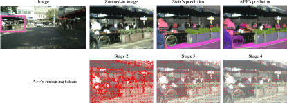
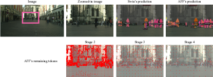
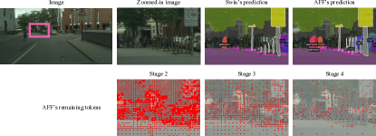
Figure 6: Additional qualitative comparison between AFF-Small and Swin-Small with Mask2Former segmentation head on Cityscapes panoptic segmentation. The red pixels in the even rows indicate the locations of the remaining tokens in stage 2, 3 and 4.

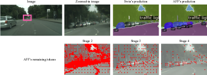
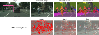
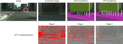
Figure 7: (Continued) Additional qualitative comparison between AFF-Small and Swin-Small with Mask2Former segmentation head on Cityscapes panoptic segmentation. The red pixels in the even rows indicate the locations of the remaining tokens in stage 2, 3 and 4.

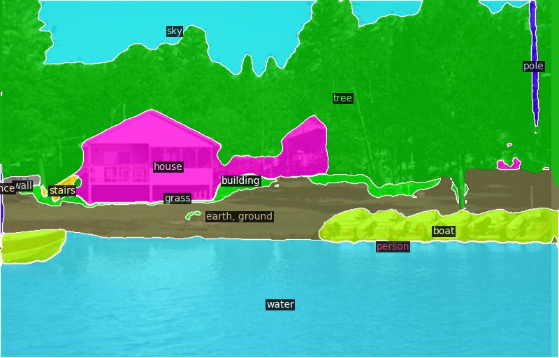
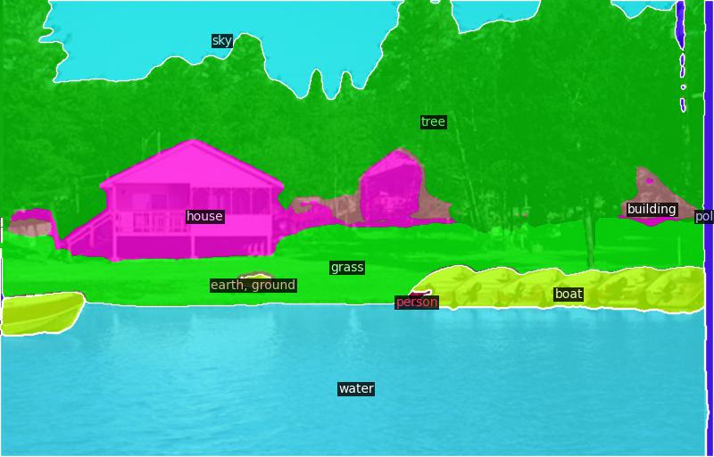
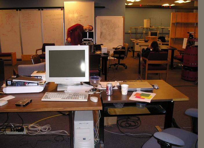
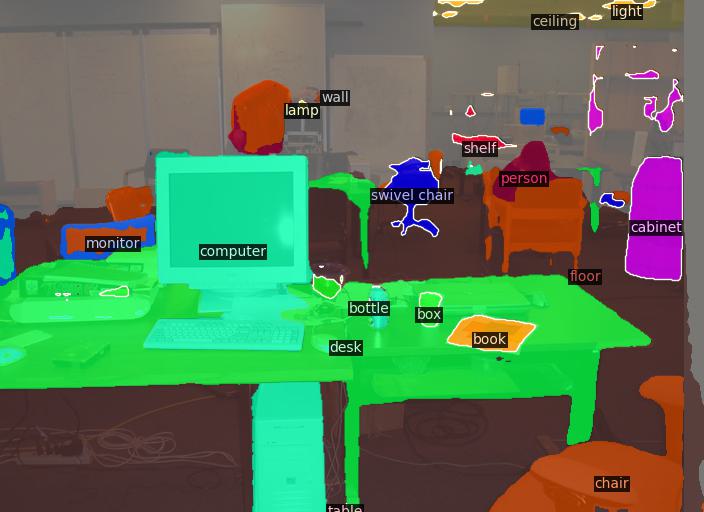
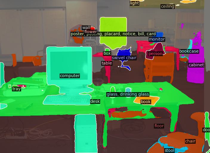
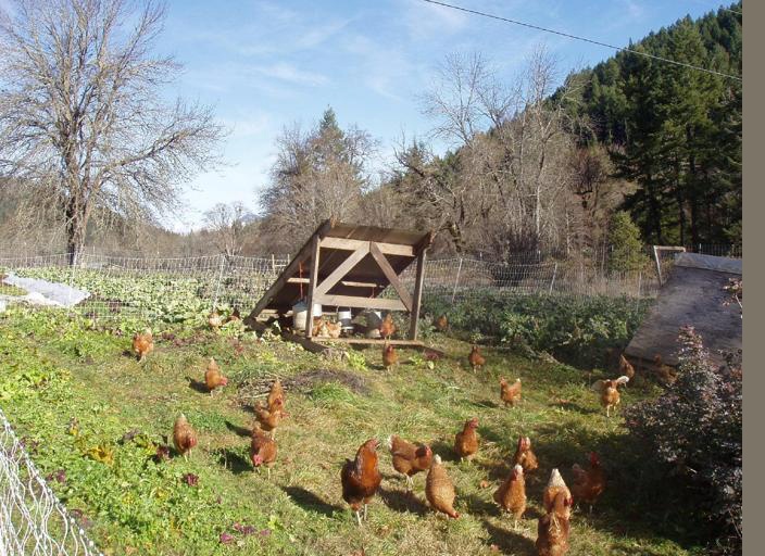
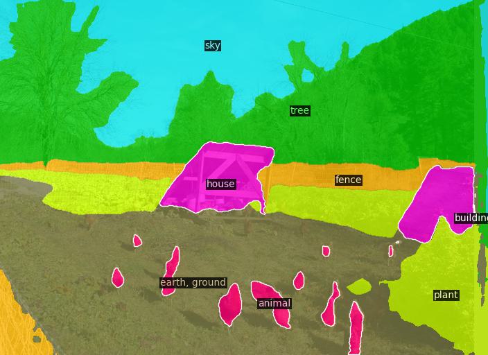
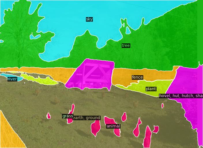
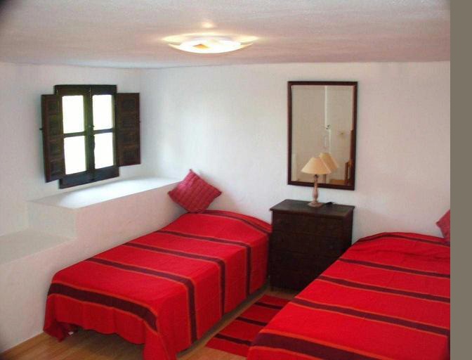
(a) Original images.

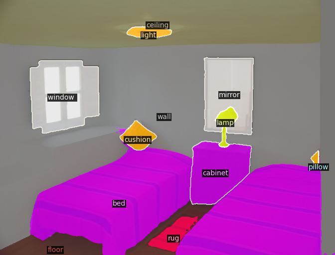
(b) AFF-Tiny predictions.

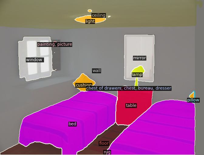
(c) Swin-Tiny prediction.

Figure 8: Qualitative comparison between AFF-Tiny and Swin-Tiny with Mask2Former segmentation head on ADE20K semantic segmentation. First column: original image. Second column: AFF prediction. Third column: Swin prediction.

References

- [1] Arindam Banerjee and Joydeep Ghosh. Scalable clustering algorithms with balancing constraints. Data Mining and Knowledge Discovery, 13(3):365–395, 2006.
- [2] Bowen Cheng, Ishan Misra, Alexander G Schwing, Alexander Kirillov, and Rohit Girdhar. Masked-attention mask transformer for universal image segmentation. In Proceedings of the IEEE Conference on Computer Vision and Pattern Recognition (CVPR), pages 1290–1299, 2022.
- [3] Marius Cordts, Mohamed Omran, Sebastian Ramos, Timo Rehfeld, Markus Enzweiler, Rodrigo Benenson, Uwe Franke, Stefan Roth, and Bernt Schiele. The cityscapes dataset for semantic urban scene understanding. In Proceedings of the IEEE Conference on Computer Vision and Pattern Recognition (CVPR), 2016.
- [4] Jia Deng, Wei Dong, Richard Socher, Li-Jia Li, Kai Li, and Li Fei-Fei. Imagenet: A large-scale hierarchical image database. In Proceedings of the IEEE Conference on Computer Vision and Pattern Recognition (CVPR), pages 248–255. Ieee, 2009.
- [5] Alexey Dosovitskiy, Lucas Beyer, Alexander Kolesnikov, Dirk Weissenborn, Xiaohua Zhai, Thomas Unterthiner, Mostafa Dehghani, Matthias Minderer, Georg Heigold, Sylvain Gelly, et al. An image is worth 16x16 words: Transformers for image recognition at scale. International Conference on Learning Representations (ICLR), 2021.
- [6] Xianzhi Du, Tsung-Yi Lin, Pengchong Jin, Golnaz Ghiasi, Mingxing Tan, Yin Cui, Quoc V Le, and Xiaodan Song. Spinenet: Learning scale-permuted backbone for recognition and localization. In Proceedings of the IEEE Conference on Computer Vision and Pattern Recognition (CVPR), pages 11592–11601, 2020.
- [7] Xianzhi Du, Barret Zoph, Wei-Chih Hung, and Tsung-Yi Lin. Simple training strategies and model scaling for object detection. arXiv preprint arXiv:2107.00057, 2021.
- [8] Haoqi Fan, Bo Xiong, Karttikeya Mangalam, Yanghao Li, Zhicheng Yan, Jitendra Malik, and Christoph Feichtenhofer. Multiscale vision transformers. In Proceedings of the IEEE International Conference on Computer Vision (ICCV), pages 6824–6835, 2021.
- [9] Mohsen Fayyaz, Soroush Abbasi Koohpayegani, Farnoush Rezaei, and Sommerlade1 Hamed Pirsiavash2 Juergen Gall. Adaptive token sampling for efficient vision transformers. In Proceedings of the European Conference on Computer Vision (ECCV), 2022.
- [10] Golnaz Ghiasi, Yin Cui, Aravind Srinivas, Rui Qian, Tsung-Yi Lin, Ekin D Cubuk, Quoc V Le, and Barret Zoph. Simple copy-paste is a strong data augmentation method for instance segmentation. In Proceedings of the IEEE Conference on Computer Vision and Pattern Recognition (CVPR), pages 2918–2928, 2021.
- [11] Benjamin Graham, Alaaeldin El-Nouby, Hugo Touvron, Pierre Stock, Armand Joulin, Hervé Jégou, and Matthijs Douze. Levit: a vision transformer in convnet’s clothing for faster inference. In Proceedings of the IEEE/CVF international conference on computer vision, pages 12259–12269, 2021.
- [12] Kaiming He, Georgia Gkioxari, Piotr Dollár, and Ross Girshick. Mask r-cnn. In Proceedings of the IEEE International Conference on Computer Vision (ICCV), pages 2961–2969, 2017.
- [13] David Hilbert. Über die stetige abbildung einer linie auf ein flächenstück. In Dritter Band: Analysis· Grundlagen der Mathematik· Physik Verschiedenes, pages 1–2. Springer, 1935.
- [14] Tao Huang, Lang Huang, Shan You, Fei Wang, Chen Qian, and Chang Xu. Lightvit: Towards light-weight convolution-free vision transformers. arXiv preprint arXiv:2207.05557, 2022.
- [15] Jeff Johnson, Matthijs Douze, and Hervé Jégou. Billion-scale similarity search with GPUs. IEEE Transactions on Big Data, 7(3):535–547, 2019.
- [16] Alexander Kirillov, Ross Girshick, Kaiming He, and Piotr Dollár. Panoptic feature pyramid networks. In Proceedings of the IEEE Conference on Computer Vision and Pattern Recognition (CVPR), pages 6399–6408, 2019.
- [17] Alexander Kirillov, Yuxin Wu, Kaiming He, and Ross Girshick. Pointrend: Image segmentation as rendering. In Proceedings of the IEEE Conference on Computer Vision and Pattern Recognition (CVPR), pages 9799–9808, 2020.
- [18] Youwei Liang, Chongjian Ge, Zhan Tong, Yibing Song, Jue Wang, and Pengtao Xie. Not all patches are what you need: Expediting vision transformers via token reorganizations. In International Conference on Learning Representations (ICLR), 2022.
- [19] Tsung-Yi Lin, Michael Maire, Serge Belongie, James Hays, Pietro Perona, Deva Ramanan, Piotr Dollár, and C Lawrence Zitnick. Microsoft coco: Common objects in context. In Proceedings of the European Conference on Computer Vision (ECCV), pages 740–755. Springer, 2014.
- [20] Ze Liu, Yutong Lin, Yue Cao, Han Hu, Yixuan Wei, Zheng Zhang, Stephen Lin, and Baining Guo. Swin transformer: Hierarchical vision transformer using shifted windows. In Proceedings of the IEEE International Conference on Computer Vision (ICCV), pages 10012–10022, 2021.
- [21] Zhuang Liu, Hanzi Mao, Chao-Yuan Wu, Christoph Feichtenhofer, Trevor Darrell, and Saining Xie. A convnet for the 2020s. In Proceedings of the IEEE Conference on Computer Vision and Pattern Recognition (CVPR), pages 11976–11986, 2022.
- [22] Ilya Loshchilov and Frank Hutter. Decoupled weight decay regularization. arXiv preprint arXiv:1711.05101, 2017.
- [23] Chris J Maddison, Andriy Mnih, and Yee Whye Teh. The concrete distribution: A continuous relaxation of discrete random variables. arXiv preprint arXiv:1611.00712, 2016.
- [24] Dmitrii Marin, Jen-Hao Rick Chang, Anurag Ranjan, Anish Prabhu, Mohammad Rastegari, and Oncel Tuzel. Token pooling in vision transformers. arXiv preprint arXiv:2110.03860, 2021.
- [25] Lingchen Meng, Hengduo Li, Bor-Chun Chen, Shiyi Lan, Zuxuan Wu, Yu-Gang Jiang, and Ser-Nam Lim. Adavit: Adaptive vision transformers for efficient image recognition. In Proceedings of the IEEE Conference on Computer Vision and Pattern Recognition (CVPR), pages 12309–12318, 2022.
- [26] Bongki Moon, Hosagrahar V Jagadish, Christos Faloutsos, and Joel H. Saltz. Analysis of the clustering properties of the hilbert space-filling curve. IEEE Transactions on knowledge and data engineering, 13(1):124–141, 2001.
- [27] Bowen Pan, Rameswar Panda, Yifan Jiang, Zhangyang Wang, Rogerio Feris, and Aude Oliva. IA-RED^: Interpretability-aware redundancy reduction for vision transformers. Advances in Neural Information Processing Systems (NeurIPS), 34:24898–24911, 2021.
- [28] Junting Pan, Adrian Bulat, Fuwen Tan, Xiatian Zhu, Lukasz Dudziak, Hongsheng Li, Georgios Tzimiropoulos, and Brais Martinez. Edgevits: Competing light-weight cnns on mobile devices with vision transformers. In Proceedings of the European Conference on Computer Vision (ECCV), pages 294–311. Springer, 2022.
- [29] Giuseppe Peano. Sur une courbe, qui remplit toute une aire plane. In Arbeiten zur Analysis und zur mathematischen Logik, pages 71–75. Springer, 1990.
- [30] Charles Ruizhongtai Qi, Li Yi, Hao Su, and Leonidas J Guibas. Pointnet++: Deep hierarchical feature learning on point sets in a metric space. Advances in Neural Information Processing Systems (NeurIPS), 30, 2017.
- [31] Prajit Ramachandran, Niki Parmar, Ashish Vaswani, Irwan Bello, Anselm Levskaya, and Jon Shlens. Stand-alone self-attention in vision models. Advances in Neural Information Processing Systems (NeurIPS), 32, 2019.
- [32] Yongming Rao, Wenliang Zhao, Benlin Liu, Jiwen Lu, Jie Zhou, and Cho-Jui Hsieh. Dynamicvit: Efficient vision transformers with dynamic token sparsification. Advances in Neural Information Processing Systems (NeurIPS), 34:13937–13949, 2021.
- [33] Tal Ridnik, Emanuel Ben-Baruch, Asaf Noy, and Lihi Zelnik-Manor. Imagenet-21k pretraining for the masses. In Thirty-fifth Conference on Neural Information Processing Systems Datasets and Benchmarks Track (Round 1), 2021.
- [34] Peter J Rousseeuw. Silhouettes: a graphical aid to the interpretation and validation of cluster analysis. Journal of computational and applied mathematics, 20:53–65, 1987.
- [35] Aurko Roy, Mohammad Saffar, Ashish Vaswani, and David Grangier. Efficient content-based sparse attention with routing transformers. Transactions of the Association for Computational Linguistics, 9:53–68, 2021.
- [36] Michael S Ryoo, AJ Piergiovanni, Anurag Arnab, Mostafa Dehghani, and Anelia Angelova. Tokenlearner: What can 8 learned tokens do for images and videos? Advances in Neural Information Processing Systems (NeurIPS), 2021.
- [37] Bharat Singh, Mahyar Najibi, and Larry S Davis. Sniper: Efficient multi-scale training. Advances in Neural Information Processing Systems (NeurIPS), 31, 2018.
- [38] Lin Song, Songyang Zhang, Songtao Liu, Zeming Li, Xuming He, Hongbin Sun, Jian Sun, and Nanning Zheng. Dynamic grained encoder for vision transformers. Advances in Neural Information Processing Systems (NeurIPS), 34:5770–5783, 2021.
- [39] Aravind Srinivas, Tsung-Yi Lin, Niki Parmar, Jonathon Shlens, Pieter Abbeel, and Ashish Vaswani. Bottleneck transformers for visual recognition. In Proceedings of the IEEE Conference on Computer Vision and Pattern Recognition (CVPR), pages 16519–16529, 2021.
- [40] Teppei Suzuki. Clustering as attention: Unified image segmentation with hierarchical clustering. arXiv preprint arXiv:2205.09949, 2022.
- [41] Apoorv Vyas, Angelos Katharopoulos, and François Fleuret. Fast transformers with clustered attention. Advances in Neural Information Processing Systems (NeurIPS), 33:21665–21674, 2020.
- [42] Shuohang Wang, Luowei Zhou, Zhe Gan, Yen-Chun Chen, Yuwei Fang, Siqi Sun, Yu Cheng, and Jingjing Liu. Cluster-former: Clustering-based sparse transformer for question answering. In Findings of the Association for Computational Linguistics: ACL-IJCNLP 2021, pages 3958–3968, 2021.
- [43] Wenhai Wang, Enze Xie, Xiang Li, Deng-Ping Fan, Kaitao Song, Ding Liang, Tong Lu, Ping Luo, and Ling Shao. Pyramid vision transformer: A versatile backbone for dense prediction without convolutions. In Proceedings of the IEEE International Conference on Computer Vision (ICCV), pages 568–578, 2021.
- [44] Wenhai Wang, Enze Xie, Xiang Li, Deng-Ping Fan, Kaitao Song, Ding Liang, Tong Lu, Ping Luo, and Ling Shao. Pvt v2: Improved baselines with pyramid vision transformer. Computational Visual Media, 8(3):415–424, 2022.
- [45] Wenxuan Wu, Zhongang Qi, and Li Fuxin. Pointconv: Deep convolutional networks on 3d point clouds. In Proceedings of the IEEE Conference on Computer Vision and Pattern Recognition (CVPR), pages 9621–9630, 2019.
- [46] Enze Xie, Wenhai Wang, Zhiding Yu, Anima Anandkumar, Jose M Alvarez, and Ping Luo. Segformer: Simple and efficient design for semantic segmentation with transformers. Advances in Neural Information Processing Systems (NeurIPS), 34:12077–12090, 2021.
- [47] Hongxu Yin, Arash Vahdat, Jose M Alvarez, Arun Mallya, Jan Kautz, and Pavlo Molchanov. A-vit: Adaptive tokens for efficient vision transformer. In Proceedings of the IEEE Conference on Computer Vision and Pattern Recognition (CVPR), pages 10809–10818, 2022.
- [48] Qihang Yu, Huiyu Wang, Siyuan Qiao, Maxwell Collins, Yukun Zhu, Hartwig Adam, Alan Yuille, and Liang-Chieh Chen. k-means mask transformer. In Proceedings of the European Conference on Computer Vision (ECCV), pages 288–307. Springer, 2022.
- [49] Weihao Yu, Mi Luo, Pan Zhou, Chenyang Si, Yichen Zhou, Xinchao Wang, Jiashi Feng, and Shuicheng Yan. Metaformer is actually what you need for vision. In Proceedings of the IEEE Conference on Computer Vision and Pattern Recognition (CVPR), pages 10819–10829, 2022.
- [50] Xiaoyu Yue, Shuyang Sun, Zhanghui Kuang, Meng Wei, Philip HS Torr, Wayne Zhang, and Dahua Lin. Vision transformer with progressive sampling. In Proceedings of the IEEE International Conference on Computer Vision (ICCV), pages 387–396, 2021.
- [51] Shuangfei Zhai, Walter Talbott, Nitish Srivastava, Chen Huang, Hanlin Goh, Ruixiang Zhang, and Josh Susskind. An attention free transformer. arXiv preprint arXiv:2105.14103, 2021.
- [52] Hengshuang Zhao, Li Jiang, Jiaya Jia, Philip HS Torr, and Vladlen Koltun. Point transformer. In Proceedings of the IEEE International Conference on Computer Vision (ICCV), pages 16259–16268, 2021.
- [53] Minghang Zheng, Peng Gao, Renrui Zhang, Kunchang Li, Xiaogang Wang, Hongsheng Li, and Hao Dong. End-to-end object detection with adaptive clustering transformer. In Proceedings of the British Machine Vision Conference (BMVC), 2021.
- [54] Bolei Zhou, Hang Zhao, Xavier Puig, Sanja Fidler, Adela Barriuso, and Antonio Torralba. Scene parsing through ade20k dataset. In Proceedings of the IEEE Conference on Computer Vision and Pattern Recognition (CVPR), pages 633–641, 2017.
- [55] Xizhou Zhu, Weijie Su, Lewei Lu, Bin Li, Xiaogang Wang, and Jifeng Dai. Deformable DETR: Deformable transformers for end-to-end object detection. In International Conference on Learning Representations (ICLR), 2021.