Recognizing and generating unswitchable graphs

Abstract

In this paper, we show that unswitchable graphs are a proper subclass of split graphs, and exploit this fact to propose efficient algorithms for their recognition and generation.

1 Introduction

Let $G=(V,E)$ be a simple graph on the vertex set $V=\{v_{1},v_{2},\ldots,v_{n}\}$. Let $d_{i}$ be the degree of $v_{i}$. Assume without loss of generality that $n-1\geq d_{1}\geq d_{2}\geq\ldots\geq d_{n}\geq 0$. There may exist many other graphs $G$ with the same degree sequence, making it a many-to-one mapping.

Let the edges $\{u,v\}$, $\{w,x\}$ of $G$ be independent (this means that the edges do not have an end-point in common). For each of the three ways the edges can be independent, we can obtain another graph $G^{\prime}$ with the same degree sequence by means of a 2-switch as shown in Figure 1, in pairs from left to right and top to bottom, where the dashed lines show the replacement edges.

Figure 1: Graph $G^{\prime}$ obtained from $G$ by a 2-switch

A graph $G$ is said to be unswitchable if it cannot be reduced to another graph $H$ with the same degree sequence by edge-switching. In this paper, we propose an algorithm for recognizing unswitchable graphs that exploits the relationship of this class of graphs to the class of split-graphs.

To motivate the significance of the concept of edge-switching we dicuss an application in the next section.

2 An application of edge-switching

Given a graph $G$, it is easy to obtain its degree sequence $d$. However, given $d$ with the $d_{i}$’s in non-increasing order, the question whether there exists a graph whose degree sequence is $d$ has spawned a lot of research. We begin with the following definition.

Definition 1

The sequence $d$ is graphical if there exists a graph $G$ such $d_{G}(v_{i})=d_{i}$ for $i=1,\ldots,n$, where $d_{G}(v_{i})$ denotes the degree of the vertex $v_{i}$ in $G$.

Both Hakimi [3] and Havel [5] are credited with the following result.

Theorem 1

Let $n\geq 2$ and $d_{1}\geq 1$. The sequence $d$ is graphical if and only if the sequence $d_{2}-1,d_{3}-1,\ldots,d_{d_{1}+1}-1,d_{d_{1}+2},d_{d_{1}+3},\ldots,d_{n}$, arranged in nonincreasing order, is graphical.

To prove this result we need a definition and prove two other results.

If a graph $H$ can be obtained from a graph $G$ by a finite sequence of 2-switches we indicate this reduction by the notation $G\stackrel{{\scriptstyle 2s}}{{\Longrightarrow}}H$. Berge [1] proved that:

Theorem 2

Two graphs $G$ and $H$ on a common vertex set $V$ satisfy $d_{G}(v)=d_{H}(v)$ for all $v\in V$ if and only if $G\stackrel{{\scriptstyle 2s}}{{\Longrightarrow}}H$.

We will invoke this result when we introduce unswitchable graphs later on. To prove Theorem 2, we first prove the following result, given a non-increasing degree sequence $d$ as above.

Theorem 3

If $G$ be a graph on $n$ vertices such that $d_{G}(v_{i})=d_{i}$, then there exists a graph $G^{\prime}$ such that $G\stackrel{{\scriptstyle 2s}}{{\Longrightarrow}}G^{\prime}$ with $N_{G^{\prime}}(v_{1})=\{v_{2},\ldots,v_{d_{1}+1}\}$.

Proof: Let $d=\Delta(G)(=d_{1})$ be the maximum vertex degree of $G$. Assume there exists a $v_{i}$ such that $\{v_{1},v_{i}\}\notin E$ for $i$ in the range $[2,d+1]$. Instead, there is an index $j\geq d+2$ such that $\{v_{1},v_{j}\}\in E$. Again, as $j>i$, according to our assumption on the degree sequence, $d_{j}\leq d_{i}$. If $V_{i}$ and $V_{j}$ are the subsets of vertices of $V$ that $v_{i}$ and $v_{j}$ are connected to respectively, $V_{i}-V_{j}\neq\emptyset$. Hence there exists $t$ such that $\{v_{i},v_{t}\}\in E$, but $\{v_{j},v_{t}\}\notin E$. Thus we can make a 2-switch so that $v_{1}$ is adjacent to $v_{i}$. We repeat this till all the vertices adjacent to $v_{1}$ have indices in the range $[2,d+1]$. $\blacksquare$

Berge’s theorem is easily proved by induction on the number of vertices of the graphs $G$ and $H$. The condition is sufficient as $G\stackrel{{\scriptstyle 2s}}{{\Longrightarrow}}H$ means that the vertex degrees are preserved. Conversely, by applying Theorem 3 to each of the graphs $G$ and $H$ we can find a vertex $v$ such that in graphs $G^{\prime}$ and $H^{\prime}$ respectively where $G\stackrel{{\scriptstyle 2s}}{{\Longrightarrow}}G^{\prime}$ and $H\stackrel{{\scriptstyle 2s}}{{\Longrightarrow}}H^{\prime}$, the neighborhood of $v$ is identical. Now the reduced graphs $G^{\prime}-v$ and $H^{\prime}-v$ have the same vertex degrees and by the induction hypothesis $G^{\prime}-v\stackrel{{\scriptstyle 2s}}{{\Longrightarrow}}H^{\prime}-v$. Consequently, $G^{\prime}\stackrel{{\scriptstyle 2s}}{{\Longrightarrow}}H^{\prime}$. Combining this with the fact that $H^{\prime}\stackrel{{\scriptstyle 2s}}{{\Longrightarrow}}H$ by a sequence of reverse 2-switches, the necessity is proved.

Here’s is an interesting application of Berge’s result. Consider the example below where we want to reduce graph $G$ to graph $H$ by 2-switches so that $v_{1}$ is adjacent to $v_{2}$ and $v_{3}$. We achieve this by switching the pair of edges $\{v_{2},v_{3}\}$, $\{v_{1},v_{4}\}$ with the non-existing pair of edges $\{v_{1},v_{3}\}$, $\{v_{2},v_{4}\}$.

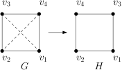
Figure 2: Graph $H$ obtained from $G$ by a 2-switch

Now, we can prove Theorem 1.

Proof: Consider the if direction. Let $G$ be a graph on $n-1$ vertices with the degree sequence:

$\langle d_{G}(v_{2})=d_{2}-1,d_{G}(v_{3})=d_{3}-1,\ldots,d_{G}(v_{d_{1}+1})=d_{d_{1}+1}-1,d_{G}(v_{d_{1}+2})=d_{d_{1}+2},d_{G}(v_{d_{1}+3})=d_{d_{1}+3},\ldots,d_{G}(v_{n})=d_{n}\rangle$

Add a new vertex $v_{1}$ and the edges $\{v_{1},v_{i}\}$ for all $i\in[2,d_{d_{1}+1}]$ . Then in the new graph $H$, $d_{H}(v_{1})=d_{1}$ , and $d_{H}(v_{i})=d_{i}$ for all $i\geq 2$.

For the only if direction, assume $d_{G}(v_{i})=d_{i}$. By the Lemma proved earlier and Berge’s result, we can assume that $N_{G}(v_{1})=\{v_{2},\ldots,v_{d_{1}+1}\}$. But now the degree sequence of $G-v_{1}$ is as above.

Example 1

The sequence $\langle 4,4,4,3,2,1\rangle$ is graphical since the following sequence of reduced sequences are each graphical: $\langle 3,3,2,1,1\rangle$, $\langle 2,1,1,0\rangle$ (this is obtained by a reordering of $\langle 2,1,0,1\rangle$, obtained from the previous sequence), $\langle 0,0,0\rangle$. The last sequence corresponds to an empty graph, and the graph corresponding to the initial sequence is easily constructed.

It should be pointed out that Hakimi’s algorithm will work if the sequence element that we choose to saturate is any element of the sequence. If its degree is $d_{i}$, we reduce the $d_{i}$ highest degree elements by 1. This observation is due to Kleitman and Wang  [6].

3 Split graphs

A graph $G$ is said to be a split graph if there exists a disjoint partition of its vertex set $V$ into a complete induced subgraph on $V_{2}$ vertices and an independent set of $V_{1}$ vertices. Fig. 3 shows an example of a split graph where the induced subgraph on the vertices $\{2,4\}$ is complete and the subset of vertices $\{1,3\}$ form an independent set.

Figure 3: A split graph

The partition of the graph into a complete graph and an independent set is not unique. For the example split graph, $\{1,2,4\}$ and $\{3\}$ is another partition into a (maximal) complete graph and an independent set.

There are other characterizations of clique graphs. For example, this: A graph $G$ is a split graph iff it does not contain any of the graphs of Figure 4 as induced subgraphs.

Figure 4: Forbidden subgraphs of a split graph

There is yet another characterization of a split graph in terms of the degrees of its vertices [4]. Let $d=(d_{1},d_{2},\ldots,d_{n})$ be the sequence of degrees of its vertices, with $n-1\geq d_{1}\geq d_{2}\geq d_{3}\geq\ldots\geq d_{n}\geq 0$. Let $m$ be the maximum index $i$ for which $d_{i}\geq i-1$. Call it the split index.

Then $G$ is a split graph iff:

$$\Sigma_{i=1}^{m}d_{i}=m(m-1)+\Sigma_{i=m+1}^{n}d_{i}$$ (1)

Thus for the example split graph of Fig. 3, we have $d=(3,3,2,2)$, $m=3$ and both sides of Eqn.(1) evaluate to 8.

This last characterization forms the basis for an easy recognition algorithm for split graphs. From the degree sequence, find the split index $m$, going left to right in the degree sequence. Construct a complete graph on $m$ vertices with degree $d_{m}$. The remaining vertices form an independent set, which are now joined to the clique vertices to saturate their degrees and the residual degrees of the clique vertices.

The forbidden subgraph characterization is of interest to us. If a split graph has a 4-cycle or its complement as an induced subgraph then it is switchable. The question is: Are all split-graphs switchable ? We explore this matter in the next section.

4 Unswitchable graphs

A $P_{4}$ is a chordless path on 4 vertices of $G$, while a $C_{4}$ is a 4-cycle and a $2K_{2}$ (the complement of a 4-cycle) is a subgraph with 2 disjoint edges of $G$.

Clearly, an unswitchable graph $G$ cannot have a $P_{4}$, a $C_{4}$ or a $2K_{2}$ as an induced subgraph on 4 vertices. Since no switching is possible, we cannot use 2-switches to transform a given graph $G$ to a graph $G^{\prime}$ with the same degree sequence.

Extrapolating from the forbidden induced subgraph characterization of unswitchable graphs, Eggleton proposed the following constructive charaterization of unswitchable graphs.

Theorem 4

[2] For any positive integer $n$, let $\{S_{i}:1\leq i\leq 2n\}$ be a family of pairwise disjoint finite (possibly empty) sets, with union $V$. Let $G$ with a vertex set $V$, such that any two distinct vertices $a\in S_{i}$ and $b\in S_{j}$, with $i\leq j$, are adjacent in $G$ just if $i+n<j$ or $i>n$. Then $G$ is unswitcahable; moreover every unswitchable graph is obtained by this construction.

Proof: (Ours) We show that the graph constructed cannot have any of the graphs $P_{4}$, $C_{4}$ or $2K_{2}$ as an induced subgraph. We argue the case of $C_{4}$. Let the labels of the vertices of $C_{4}$ be $a,b,c,d$ in cyclic order. Since $a$ and $c$ are not connected both cannot be in sets with indices greater than $n$. Let $a$ be in a set $S_{i}$ with index $i\leq n$. Since $a$ is joined to both $b$ and $d$ they are in sets $S_{j}$ and $S_{k}$ with indices greater than $i+n$. Thus $b$ and $d$ must be connected. This contradicts the assumption that the induced graph on $a,b,c,d$ is a $C_{4}$.

Similar argumemts can be made for the non-existence of $2K_{2}$ and $P_{4}$ as induced subgraphs.

Now for the second half of the theorem. Let $G$ be a given unswitchable graph. Since it is a split graph, let there be $m$ edges connecting a vertex of the independent set with a vertex of the clique. If $\{u,v\}$ is one such edge, let $u\in S_{i_{1}}$ and $v\in S_{j_{1}}$. Then we must have $j_{1}-i_{1}>n$. Thus we have $m$ such inequalities corresponding to the $m$ edges.

Further, $j_{1}>n$ and $i_{1}\leq n$ for each pair of indices corresponding to the $m$ edges. This means that we have to choose $m$ pairs of points in the polygonal region in the $x-y$ plane bounded by the lines $x-y>n$, $x>n$ and $y\leq n$.

We choose a minimum $n$ such that $m$ pairs of points can be found in this polygonal region. For the unswitchable graph of Figure 5 a distribution of its vertices among the sets $S_{i}$ is shown in Figure 6 $\blacksquare$

Following the theorem, we constructed the unswitchable graph shown in Figure 5, setting $n=2$.

Figure 5: A non-switchable graph $G_{1}$

The sets $S_{i}$, the membership of the vertices in these sets and the mutual adjacencies of the vertices are shown in Figure 6.

Figure 6: Set distribution of the vertices of $G_{1}$

Here’s another example, where we have gone in the opposite direction, setting $n=2$ again and constructing the sets $S_{i}$, for $i=1,2,\ldots,2n$, and adding edges between vertices in pairs of sets $S_{i}$ and $S_{j}$ for $i\leq j$, satisfying the other constraints on $i$ and $j$.

Figure 7: Distribution of the vertices among the sets $S_{i}$

Both the graphs of Figure 5 and Figure 7 are split-graphs. This leads us to speculate on what might be the relationship between these two graph classes: split-graphs and unswitchable graphs.

Figure 8: A split graph that is switchable

It appears that the class of split graphs has an overlap with the class of unswitchable graphs. As evidence we have the graphs of Figure 5 and Figure 7 which are split graphs but not switchable. On the other hand the graph of Figure 8 is a split graph but switchable as there exist several $P_{4}$’s as induced subgraphs.

An interesting problem is to construct a switchable graph that is not a split graph. Consider a graph $G$ consisting of two copies of the graph of Figure 5. This graph is not a split graph but it is switchable. Indeed by running our implementation of Hakimi’s algorithm on the degree sequence $d=(5,5,5,5,5,5,3,3,3,3,3,3)$ we obtained the graph of Figure 9 as output. This is not a split graph as there is an induced 4-cycle on the vertex set $\{2,3,9,10\}$ and is a switchable graph for the same reason.

The above considerations lead us to make the following claim.

Claim 1

Unswitchable graphs are a proper subclass of split graphs.

Proof: This is true since the graphs defined by Eggleton’s result are all split graphs. The vertices in the sets with indices at most $n$ constitute an independent set and the ones with indices greater than $n$ form a complete graph. The inclusion is proper since we have found a split graph that is switchable (Figure 8). $\blacksquare$

Figure 9: A graph that is switchable but not split

In view of Claim 1, we can design a recognition algorithm for unswitchable graphs. Given an input graph, we first run a recognition algorithm for split graphs (for example, the degree sequence based recognition algorithm mentioned in the previous section) and if the output is true, check that the graph does not have a $P_{4}$ as an induced subgraph. For this we proceed as follows.

The recognition algorithm returns a split index $m$ as discussed in the Section 3 so that the vertices with degrees $d_{m+1}\geq d_{m+2}\geq\ldots\geq d_{n}$ constitute an independent set. Knowing this, from the adjacency list of the input graph, we find the adjacency list of each vertex of the independent set (Figure 10).

We use this information to construct another adjacency list that gives for each vertex of the complete graph the vertices of the independent set that are adjacent to it.

Now, for an edge $\{u,v\}$ of the clique we can find the sets of vertices $S_{u}$ and $S_{v}$ of the independent set that are adjacent to $u$ and $v$ respectively. If the set differences $S_{u}-S_{v}$ and $S_{v}-S_{u}$ are both nonempty then there exists a path $P_{4}$ betweeen $u$ and $v$, making the graph switchable. If there exists no clique edge $\{u,v\}$ for which this is true then the graph is unswitchable.

Consider the graph of Figure 5 without the edges 2-6 and 3-5. The adjacency list for the vertices of the independent set and the adjacency list for the vertices of the complete graph derived from it are shown in Figure 10.

Figure 10: Adjacency Lists for the modified Graph of Fig. 5

For the edge $u$-$v$ = 6-5, $S_{u}=\{1,3\}$ and $S_{v}=\{1,2\}$. The set differences are $\{2\}$ and $\{3\}$. Since these are both non-empty, there is a $P_{4}$ path: 3-6-5-2. This shows that the modified graph is switchable.

A formal description of the recognition algorithm is given below. The time complexity of the recognition of the algorithm is $O(n_{1}n_{2}^{2})$, where $n_{1}$ and $n_{2}$ are respectively the sizes of the independent set and the clique set. Since $n_{1}$ and $n_{2}$ are both bounded by $n$, $O(n^{3})$ is a more succinct description of the complexity of the algorithm.

Algorithm 1 UnswitchableGraphRecognition$(G)$

Input: The adjacency lists of the vertices of a graph $G$
Output: $G$ is switchable or not

1:Extract the degree sequence, $d=d_{1}\geq d_{2}\geq\ldots\geq d_{n}$ of $G$

2:output $\leftarrow$ Run the recognition algorithm for a split-graph on $d$

3:if (output = YES) then

4:     Let $m$ be the split index

5:     Extract adjacency lists of the vertices with degrees $\geq d_{m+1}$

6:     for each edge $u-v$ of the complete graph on the vertices with degrees $\leq d_{m}$: do

7:         Compute the neighborhoods $S_{u}$ and $S_{v}$ of the end points in the independent set

8:         Compute $S_{u}-S_{v}$ and $S_{v}-S_{u}$.

9:         if $S_{u}-S_{v}$ and $S_{v}-S_{u}$ are disjoint and non-empty: then

10:              return “G is switchable”

11:         else continue

12:         end if

13:     end for

14:     return “G is unswitchable”

15:else

16:     return “G is switchable”

17:end if

5 Generating an unswitchable graph

The second half of the proof of Eggleton’s theorem requires an unswitchable graph as input. We would also like to test the recognition algorithm of the previous section on instances of unswitchable graphs. Motivated by these applications, we consider the problem of generating an unswitchable graph on $n$ vertices by an independent method.

We first generate a split graph. Let $n$ be the number of vertices $V$ of the graph, obtained as (user) input. We partition $V$ into two disjoint non-empty subsets $V_{1}$ and $V_{2}$ of size $n_{1}$ and $n_{2}$ respectively. We assume that $n_{2}\geq 2$ to avoid trivial cases. Construct a complete graph on the vertices of $V_{2}$. For each of the remaining $n_{1}$ vertices of $V_{1}$, choose a random integer $p$ in the range [0, $n_{2}$] and join the chosen vertex to a random subset of vertices of $V_{2}$ of size $p$.

We now proceed as in the algorithm for recognizing a split graph with a small change. For each pair of vertices $\{u,v\}$ in the independent set $V_{1}$, we determine the set of neighbors $S_{u}$ and $S_{v}$ in the set of clique vertices $V_{2}$. Compute the difference sets $S_{u}$-$S_{v}$ and $S_{v}$-$S_{u}$. If these are non-empty and disjoint, for each pair of vertices $x$ and $y$ in the difference sets we have a $P_{4}$, defined by $u$-$x$-$y$-$v$.

A formal algorithm for generating these $P_{4}$’s is described below. If no induced subgraph isomorphic to a $P_{4}$ has been found, then we have an unswitchable graph. Othewise, we introduce new edges (chords) to eliminate the $P_{4}$’s. This in turn will generate new $P_{4}$’s formed by pairs of the newly introduced chords. Once again chords are introduced to eliminate the new $P_{4}$’s. We continue until only one new $P_{4}$ is generated.

Algorithm 2 findP4s

1:Input: Adjacency list of graph $G$ and vertices of the independent set $V_{1}$

2:Output: List of all $P_{4}$s in $G$

3:procedure find_all_P4s($adjacency\_list,V_{1}$)

4:     $ListP4\leftarrow[]$

5:     for each pair of vertices $v_{1}$ and $v_{2}$ in $V_{1}$  do

6:         $S_{1}\leftarrow$ set of neighbours of $v_{1}$ read from $adj\_list$

7:         $S_{2}\leftarrow$ set of neighbours of $v_{2}$ read from $adj\_list$

8:         $S_{12}\leftarrow S_{1}-S_{2}$

9:         $S_{21}\leftarrow S_{2}-S_{1}$

10:         if both $S_{12}$ and $S_{21}$ are non-empty then

11:              for each pair $a,b$ where $a\in S_{12}$ and $b\in S_{21}$  do

12:                  Add $[v_{1},a,b,v_{2}]$ to $ListP4$

13:              end for

14:         end if

15:     end for

16:     return $ListP4$

17:end procedure

Consider the example of Figure 11, where $V_{1}=\{a,b\}$ and $V_{2}=\{1,2,3,4\}$. Apart from the edges of the clique on $V_{2}$, we have introduced edges $\{a1\}$, and $\{b2,b3,b4\}$.

Figure 11: First step in generating an unswitchable graph

For each one of the edges of the clique we consider the induced $P_{4}$ formed with pairs of vertices in the set $V_{1}=\{a,b\}$. There are three of them as shown in Figure 12.

Figure 12: Second step in generating an unswitchable graph

These induced subgraphs can be taken care of by introducing one the edges in $\{a2,b1\}$, $\{a3,b1\}$ and $\{a2,b1\}$ in the induced $P_{4}$’s from left to right. All three can be taken care of by introducing the edge $b1$ in the three induced $P_{4}$’s. The updated graph is shown in Figure 13, with the newly added edge as a dashed segment.

Figure 13: Third step in generating an unswitchable graph

We immediately see that this as a problem of finding minimum cover for a class of 2-element sets in the general case. We have to go further.

Introducing these new edges can give rise to new induced $P_{4}$’s. These are found by examining pairs of newly introduced edges and checking whether a $P_{4}$ is induced by these edges and the edge joining their end points in the set $V_{2}$. Once again, we generate a class of 2-element sets, for which we solve a minimum cover problem. We continue this iteratively, until we reach a stage when we have a cover of size one.

In the chosen example above, the process comes to an end in one step.

We describe formally the algorithms to generate an instance of the vertex cover problem introduced at each stage and since it is an NP-complete problem a minimum-vertex degree heuristic used to add as few chords as possible to eliminate the $P_{4}$’s.

Algorithm 3 vertexCoverInstanceGeneration

1:Input: $ListP4$ from $G$

2:Output: An ordered dictionary with the two vertices that define a chord as key and value the frequency of occurrences of the chord.

3:procedure find_all_2_element_sets($ListP4$)

4:     $two\_element\_set\_count\leftarrow\{\}$

5:     for each $e\in ListP4$ do

6:         $two\_element\_inst\_one\leftarrow$ first and third element of $e$

7:         $two\_element\_inst\_two\leftarrow$ second and fourth element of $e$

8:         if $two\_element\_inst\_one$ is present in $two\_element\_set\_count$ then

9:              Increment the value by 1 for key $two\_element\_inst\_one$

10:         else

11:              Set the value to 1 for key $two\_element\_inst\_one$

12:         end if

13:         if $two\_element\_inst\_two$ is present in $two\_element\_set\_count$ then

14:              Increment the value by 1 for key $two\_element\_inst\_two$

15:         else

16:              Set the value to 1 for key $two\_element\_inst\_two$

17:         end if

18:     end for

19:     Sort $two\_element\_set\_count$ in decreasing order of values

20:     return $two\_element\_set\_count$

21:end procedure

Algorithm 4 edgeAddition

1:Input: Current edge list of graph $G$, $ListP4$ and $V_{1}$

2:Output: List of new edges added to make $G$ unswitchable.

3:procedure add_min_edges($edge\_list$, $ListP4$, $V_{1}$)

4:     $edge\_list\_copy\leftarrow$ Copy current $edge\_list$

5:     $new\_edge\_list\leftarrow[]$

6:     while $ListP4$ is not empty do

7:         $two\_element\_counts\leftarrow$ find_all_2_element_sets($ListP4$)

8:         $vertices\_to\_add\leftarrow$ first element of $two\_element\_counts$

9:         Add the extracted vertices from $vertices\_to\_add$ to $edge\_list\_copy$

10:         Add the extracted vertices from $vertices\_to\_add$ to $new\_edge\_list$

11:         $adjacency\_list\leftarrow$ Convert $edge\_list\_copy$ to adjacency list

12:         $ListP4\leftarrow$ find_all_p4s($adjacency\_list$, $V_{1}$)

13:     end while

14:     return $new\_edge\_list$

15:end procedure

Finally, we put everything together and describe formally our algorithm for generating an unswitchable graph.

Algorithm 5 unswitchableGraphGeneration

1:Input: Number of vertices, $n_{1}$, in independent set $V_{1}$ and number of vertices, $n_{2}$, in clique set $V_{2}$

2:Output: An edge_list describing the graph $G$.

3:procedure generate_unswitchable_graph_for($n_{1}$, $n_{2}$)

4:     $edge\_list\leftarrow[]$

5:     Add edges corresponding to the vertices in clique set to edge_list

6:     $count\_in\_V_{1}\leftarrow$ Pick random number of vertices in $V_{1}$ to connect to $V_{2}$

7:     while $count\_in\_V_{1}$ do

8:         $vertex\_V_{1}\_index\leftarrow$ Pick a random vertex from $V_{1}$

9:         $vertices\_count\_to\_connect\leftarrow$ Pick a random number of vertices of $V_{2}$ to connect

10:         while $vertices\_count\_to\_connect$ do

11:              $vertex\_V_{2}\_index\leftarrow$ Pick a random vertex in clique set

12:              $edge\leftarrow$ ($vertex\_V_{1}\_index$, $vertex\_V_{2}\_index$)

13:              if $edge$ not in edge_list then

14:                  Add the edge to $edge\_list$ and decrement $vertices\_count\_to\_connect$

15:              end if

16:         end while

17:         Decrement $count\_in\_V_{1}$

18:     end while

19:     $adjacency\_list\leftarrow$ Convert $edge\_list$ to adjacency list

20:     $new\_edge\_list\leftarrow[]$

21:     $ListP4\leftarrow$ find_all_p4s($adjacency\_list$, $V_{1}$)

22:     if number of $p4s>0$ then

23:         $new\_edge\_list\leftarrow$ add_min_edges($edge\_list$, $ListP4$, $V_{1}$)

24:     end if

25:     Concatenate $new\_edge\_list$ to $edge\_list$

26:     return $edge\_list$ that corresponds to unswitchable graph $G$

27:end procedure

Now that we have discussed a method for generating unswitchable graphs, it is instructive to choose an $n$ and construct sets $S_{1},S_{2},\ldots,S_{n}$, distributing the vertices of the graph in these sets so that the adjacencies are exactly the same as in the graph of Figure 13.

Set $n=6$ and define the sets $S_{i}$ as follows: $S_{1}=\{b\}$, $S_{2}=\{a\}$, $S_{3}=S_{4}=\{\}$, $S_{5}=\{2,3,4\}$ and $S_{6}=\{1\}$. From Eggleton’s theorem the adjacencies of the vertices in these sets are as shown in Figure 14 and we have the same graph as in Figure 13.

Figure 14: Construction of the graph of Figure 13 by applying Eggleton’s theorem

Let $N=\#P_{4}$ the number of $P_{4}$’s discovered in the first step of the vertex cover algorithm. The time complexity of the generation algorithm is then $O(n^{3}+N^{2})$, where the term $n^{3}$, as in the recognition algorithm, accounts for the time complexity of identifying the $P_{4}$’s and the second term is the sum obtained by adding a sequence of $P_{4}$’s starting with $N$ and decreasing to one, each term being an upper bound on the size of the vertex cover problem to be solved.

6 Conclusions

In this note we have proposed an algorithm for recognizing unswitchable graphs, by first showing that unswitchable graphs are a subclass of split graphs. The second half of the proof of Eggleton’s theorem requires an unswitchable graph as input. Motivated by this, we have proposed an interesting algorithm for generating unswitchable graphs. The third author has implemented both the algorithms in Python 3. In the light of Theorem 2, the degree sequence of an unswitchable graph is uniquely realizable.

A challenging open problem is to design an algorithm for generating an unswitchable graph on $n$ vertices uniformly at random.

References

- [1] C. Berge. Graphs and Hypergraphs. North-Holland, 1973.
- [2] R. B. Eggleton. Graphic sequences and graphic polynomials: a report. In Colloq. Math. Soc. J. Bolyai, volume 10, pages 385–392, 1975.
- [3] S. Hakimi. On the realizability of a set of integers as degrees of the vertices of a graph. SIAM J. Appl. Math., 10:496–506, 1962.
- [4] P. L. Hammer and B. Simeone. The splittance of a graph. Combinatorica, 1:275–284, 1981.
- [5] V. Havel. A remark on the existence of finite graphs (Czech.). C̆asopis Pĕst. Mat., 80:477–480, 1955.
- [6] D. J. Kleitman and D. L. Wang. Algorithms for constructing graphs and digraphs with given valences and factors. Discret. Math., 6(1):79–88, 1973.