Abstract

We present a partial-differential-equation-based optimal path-planning framework for curvature constrained motion, with application to vehicles in 2- and 3-spatial-dimensions. This formulation relies on optimal control theory, dynamic programming, and a Hamilton-Jacobi-Bellman equation. Many authors have developed similar models and work employed grid-based numerical methods to solve the partial differential equation required to generate optimal trajectories. However, these methods can be inefficient and do not scale well to high dimensions. We describe how efficient and scalable algorithms for solutions of high dimensional Hamilton-Jacobi equations can be developed to solve similar problems very efficiently, even in high dimensions, while maintaining the Hamilton-Jacobi formulation. We demonstrate our method with several examples.

1 Introduction

In this manuscript, we develop a Hamilton-Jacobi partial differential equation (PDE) based method for optimal trajectory generation, with special application to so-called Dubins vehicles which exhibit curvature constrained motion. Specifically, we study kinematic models for simple cars, airplanes, and submarines.

Curvature constrained motion was first considered by Dubins [1] who considered a simple vehicle which could only move forward. The model was extended by Reeds and Shepp to a car which could move forward and backward [2]. In both cases, the strategy was to decompose paths into straight line segments and arcs of circles and analyze which combinations could be optimal. Later work in this direction was devoted to adding obstacles [3], and developing algorithms which can produce approximately optimal paths which are robust to perturbation [4].

To the authors’ knowledge the problem was first analyzed using dynamic programming and PDE by Takei, Tsai and others [5, 6]. Besides their work, there is a strong precedent in the literature for control theoretic, PDE-based optimal path-planning in a number of applications [7, 8, 9, 10, 11, 12, 13, 14]. Trajectory generation methods which are rooted in PDE have the advantage that they are easy to implement, entirely interpretable, and can provide theoretical guarantees regarding optimality, robustness, and other concerns. This is to distinguish them from sampling and learning based algorithms (for example [15, 16, 17, 18, 19]) which often sacrifice interpretability for efficiency. The main drawbacks of the PDE-based methods are the lack of efficiency and scalability. Because these methods typically rely on discretizing a domain and approximating a solution to a Hamilton-Jacobi PDE, they can be inefficient even for relatively low-dimensional problems, and are entirely intractable for motion planning problems whose state space is more than three dimensions. However, recent work has been devoted to developing grid-free numerical methods based on Hopf-Lax formulas which can approximate solutions to Hamilton-Jacobi equations efficiently even in high-dimensions [20, 21, 22].

In this paper, we present an optimal path-planning method for simple vehicles which maintains the Hamilton-Jacobi PDE formulation, but is very efficient even for problems with high-dimensional state spaces. This requires a reformulation of the standard control theoretic minimal-time path-planning problem analyzed in [5, 6, 10, 11, 12, 13, 14]. Our method represents a significant step toward fully interpretable PDE-based motion-planning algorithms which are real-time applicable.

The paper is laid out as follows. In section 2, we present the basic dynamic programming and PDE-based path-planning framework that we use, and introduce models for simple Dubins’ type vehicles. In section 3, we discuss the numerical methods which we use to solve the requisite PDEs and generate optimal trajectories, and their specific application to our problem. In section 4, we present results of our simulation. We conclude with a brief discussion of our method and potential future research directions in section 5.

2 Modeling

In this section, we derive the PDE-based path-planning algorithms which we use. In particular, because we will solve these PDEs by translating them into optimization problems, it will be most convenient if we can avoid a formulation which requires boundary conditions, which would translate into difficult constraints in the optimization. Because of this, we opt for a level-set-type formulation in the vein of [7, 8, 9], as opposed to the control theoretic approach of [5, 6, 10, 11, 12, 13, 14]. These approaches are compatible, but different in philosophy. We compare and contrast them later.

The level-set method is a general method for modeling contours (or more generally, hypersurfaces of codimension 1) which evolve with prescribed velocity depending on the ambient space and properties inherent to the contour itself [23, 24]. The basic strategy is to model the contour as the zero level set of an auxiliary function $u:\mathbb{R}^{n}\times[0,\infty)\to\mathbb{R}$ and derive a PDE which $u$ satisfies. As $u$ evolves according to the PDE, the zero level set of $u(\cdot,t)$ evolves, affecting the level set flow. A general, first-order level set equation has the form

$$u_{t}+H(t,x,\nabla u)=0$$

for some Hamiltonian function $H(t,x,p)$ which is homogeneous of degree 1 in the variable $p$. The level set function $u$ does not need to have any physical meaning, though in many cases (as in ours), level set equations are seen to arise as Hamilton-Jacobi-Bellman equations for feedback control problems where $u$ is a value function.

We demonstrate this with a brief and formal derivation. Given a time-horizon $T>0$, a starting location $x_{0}\in\mathbb{R}^{d}$, a desired-ending location $x_{f}\in\mathbb{R}^{d}$, and a function $f:\mathbb{R}^{d}\times[0,T]\times\mathbb{R}^{m}\to\mathbb{R}^{d}$, we consider trajectories $\bm{x}:[0,T]\to\mathbb{R}^{d}$ satisfying

$$\begin{split}&\dot{\bm{x}}=f(\bm{x},t,\bm{\alpha}),\hskip 28.45274pt0<t\leq T,\\ &\bm{x}(0)=x_{0}.\end{split}$$ (1)

Here $\bm{\alpha}(\cdot)$ is a control map, taking values in some admissible control set $A\subset\mathbb{R}^{m}$. The goal is to choose $\bm{\alpha}(\cdot)$ so as to steer the trajectory as close as possible to $x_{f}$ by time $T$. That is, defining the cost functional

$$\mathcal{C}[\bm{x}(\cdot)]=\left\lvert\bm{x}(T)-x_{f}\right\rvert,$$

we would like to solve the optimization problem

$$\inf_{\bm{\alpha}\in\mathcal{A}}\mathcal{C}[\bm{x}(\cdot)]$$

where $\mathcal{A}$ is the set of measurable functions from $[0,T]$ to $A.$

For $x\in\mathbb{R}^{d}$ and $t\in[0,T)$, we define the value function

$$u(x,t)=\inf_{\bm{\alpha}}\mathcal{C}_{x,t}[\bm{x}(\cdot)],$$

where $\mathcal{C}_{x,t}$ denotes the same functional restricted to trajectories $\bm{x}(\cdot)$ such that $\bm{x}(t)=x$. This value function denotes the minimum distance to the desired endpoint that one can achieve if they are sitting at point $x$ at time $t$. In our case, because there is no running cost along the trajectory, the dynamic programming principle [25] states that the value function is constant along an optimal trajectory. That is, for $\delta>0$,

$$u(\bm{x}(t),t)=\inf_{\bm{\alpha}}\{u(\bm{x}(t+\delta),t+\delta)\},$$

where the infimum is taken with respect to the values of $\bm{\alpha}(s)$ for $s\in[t,t+\delta)$. If $u$ is smooth, we rearrange, divide by $\delta$ and send $\delta\to 0^{+}$ to see

$$\inf_{\alpha\in A}\{u_{t}+\langle\dot{\bm{x}},\nabla u\rangle\}=0.$$

We can use the equation of motion (1) to replace $\dot{\bm{x}}$. Further, at time $t=T$, there is no remaining time to travel, so the value is simply the exit cost. Thus we arrive at a terminal-valued Hamilton-Jacobi-Bellman equation

$$\begin{split}&u_{t}+\inf_{\alpha\in A}\{\langle f(x,t,\alpha),\nabla u\rangle\}=0,\\ &u(x,T)=\left\lvert x-x_{f}\right\rvert.\end{split}$$ (2)

These computations are entirely formal. There is no reason to believe that $u$ will be smooth, but under very mild conditions on $f$, $u$ will be the Lipschitz continuous viscosity solution of (2) [26, 27, 28]. Assuming the viscosity solution to (2) is known, one resolves the optimal control map via

$$\bm{\alpha}^{*}(x,t)=\operatorname*{arg\,min}_{\alpha\in A}\langle f(x,t,a),\nabla u(x,t)\rangle.$$

Again, pending mild assumptions on $f$, this optimization problem has a unique solution whenever $\nabla u(x,t)$ exists, which is true for almost every $(x,t)$ when $u$ is Lipschitz continuous. Finally, one can then resolve the optimal trajectory by integrating

$$\begin{split}&\dot{\bm{x}}=f(\bm{x},t,\bm{\alpha}^{*}(\bm{x},t)),\hskip 28.45274pt0<t\leq T,\\ &\bm{x}(0)=x_{0},\end{split}$$ (3)

or using a semi-Lagrangian method as described in [6, 11, 14].

Because we will solve (2) using Hopf-Lax time formulas (and because it is more comfortable for those familiar with PDE), we make the substitution $t\mapsto T-t$, to arrive at an initial value Hamilton-Jacobi-Bellman equation:

$$\begin{split}&u_{t}-\inf_{\alpha\in A}\{\langle f(x,t,\alpha),\nabla u\rangle\}=0,\\ &u(x,0)=\left\lvert x-x_{f}\right\rvert.\end{split}$$ (4)

For notational convenience, we will still refer to the solution of (4) as $u$, though it is a time-inverted version of the solution of (2).

In the ensuing subsections, we use this basic framework to develop optimal path-planning algorithms for Dubins vehicles in 2- and 3-dimensions.

2.1 Dubins Car

We consider a simple rectangular car as pictured in figure 1. We let $(x,y)\in\mathbb{R}^{2}$ denote the center of mass of the car and $\theta\in[0,2\pi]$ denote the orientation, measured counterclockwise from the horizontal. We refer to $(x,y,\theta)$ as the configuration of the car. The car has a rear axle of length $2R$ and distance $d$ from the center of mass to the center of the rear axle. The motion of the car is subject to the nonholonomic constraint

$$\dot{y}\cos{\theta}-\dot{x}\sin{\theta}=d\dot{\theta}$$ (5)

which specifies that movement occurs tangential to the rear wheels. Motion is also constrained by a maximum angular velocity $|\dot{\theta}|\leq W$ (or equivalently a minimum turning radius $\rho=1/W$). The kinematics for the car are given by:

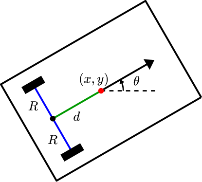
Figure 1: A simple self-driving car

$$\begin{split}&\dot{\bm{x}}=\bm{v}\cos{\bm{\theta}}-\bm{\omega}Wd\sin{\bm{\theta}},\\ &\dot{\bm{y}}=\bm{v}\sin{\bm{\theta}}+\bm{\omega}Wd\cos{\bm{\theta}},\\ &\dot{\bm{\theta}}=\bm{\omega}W.\end{split}$$ (6)

Here, $\bm{v}(\cdot),\bm{\omega}(\cdot)\in[-1,1]$ are normalized control variables representing tangential and angular velocity, respectively.

Given a desired final configuration $(x_{f},y_{f},\theta_{f})$ for the car, we can insert these dynamics into the above derivation so that the (time-reversed) optimal remaining distance function $u(x,y,\theta,t)$ for this problem satisfies the Hamilton-Jacobi-Bellman equation

$$u_{t}-\inf_{v,\omega}\Big{\{}u_{x}(v\cos\theta-\omega Wd\sin\theta)+u_{y}(v\sin\theta+\omega Wd\cos\theta)+\omega Wu_{\theta}\Big{\}}=0.$$

Rearranging to isolate $v,\omega$, we have

$$u_{t}-\inf_{v,\omega}\Big{\{}v(u_{x}\cos\theta+u_{y}\sin\theta)+\omega Wd(-u_{x}\sin\theta+u_{y}\cos\theta+\tfrac{1}{d}u_{\theta})\Big{\}}=0.$$

We recall that the control variables $v,\omega$ are normalized: $v,\omega\in[-1,1]$. Thus since the above infimum is linear in $v$ and $\omega$ and their dependence is decoupled, the infimum for each control variable must occur at one of the endpoints. Indeed, assuming $u(x,y,\theta,t)$ is known, the optimal controls are given by

$$\begin{split}v^{*}(x,y,\theta,t)&=-\text{sign}(u_{x}(x,y,\theta,t)\cos\theta+u_{y}(x,y,\theta,t)\sin\theta),\\ \omega^{*}(x,y,\theta,t)&=-\text{sign}(-u_{x}(x,y,\theta,t)\sin\theta+u_{y}(x,y,\theta,t)\cos\theta+\tfrac{1}{d}u_{\theta}).\end{split}$$ (7)

and

$$\begin{split}&u_{t}+|u_{x}\cos{\theta}+u_{y}\sin{\theta}|+Wd|-u_{x}\sin{\theta}+u_{y}\cos{\theta}+\tfrac{1}{d}u_{\theta}|=0,\\ &u(x,y,\theta,0)=|(x,y,\theta)-(x_{f},y_{f},\theta_{f})|.\end{split}$$ (8)

When modeling the car as a point mass (i.e. setting $d=0$), (8) simplifies to

$$u_{t}+|u_{x}\cos{\theta}+u_{y}\sin{\theta}|+W|u_{\theta}|=0.$$ (9)

We will deal with this latter formulation (i.e., $d=0$) so that we are neglecting the actual shape of the vehicle as in [5, 6]. Note that, as presented, we have not yet accounted for obstacles. It is argued in [10, 11] that it is easier to account for obstacles when one does not simplify the car to a point mass, but the formulation is slightly different in those papers, and we will need to make special considerations for obstacles regardless. We discuss this further in section 2.4. In the next two subsections, we present two higher dimensional generalizations of this model.

2.2 Dubins Airplane

We generalize to the case of a simple airplane by introducing a third spatial variable to the dynamics. As a result the autonomous vehicle operates in the coordinates $(x,y,z,\theta)$, rather than just $(x,y,\theta)$. This is achieved by adding in a fourth kinematic equation, which applies a restriction to the motion in the $z$ direction akin to that imposed on $\theta$. For the sake of this model, the constraint imposed on $z$ is decoupled from the constraint on the planar motion, in a manner similar to that of an airplane so we call this the Dubins Airplane model, though, as in the case of the car, we are simplifying the dynamics compared to that of a real airplane. We once again consider the vehicle to be a point mass. This leads to the kinematic equations

$$\begin{split}&\dot{\bm{x}}=\bm{v}\cos{\bm{\theta}},\\ &\dot{\bm{y}}=\bm{v}\sin{\bm{\theta}},\\ &\dot{\bm{\theta}}=\bm{\omega_{xy}}W_{xy},\\ &\dot{\bm{z}}=\bm{\omega_{z}}W_{z},\end{split}$$ (10)

where, once again, we enforce $\bm{v}(\cdot),\bm{\omega}_{xy}(\cdot),\bm{\omega}_{z}(\cdot)\in[-1,1]$. In (10), $W_{xy}>0$ is a constraint on the angular velocity in the $xy$-plane, and $W_{z}>0$ is a constraint on the angular velocity in the vertical direction.

Similar reasoning will lead us to the Hamilton-Jacobi-Bellman equation

$$\begin{split}&u_{t}+|u_{x}\cos{\theta}+u_{y}\sin{\theta}|+W_{xy}|u_{\theta}|+W_{z}|u_{z}|=0,\\ &u(x,y,z,\theta,0)=|(x,y,z,\theta)-(x_{f},y_{f},z_{f},\theta_{f})|.\end{split}$$ (11)

To truly model an airplane in flight, it makes sense to restrict to unidirectional velocity: $\bm{v}(\cdot)=1$. In this case, the equation simplifies to

$$u_{t}-u_{x}\cos{\theta}-u_{y}\sin{\theta}+W_{xy}|u_{\theta}|+W_{z}|u_{z}|=0.$$ (12)

As mentioned above, this formulation does not yet account for the presence of obstacles, which will be discussed in section 2.4. One could also account for finer-scale modeling concerns such as minimum cruising velocity, but for our purposes, the formulation is as presented.

2.3 Dubins Submarine

As an alternative to Dubins Airplane, we can model the problem in three dimensions by enforcing a total curvature constraint, rather than decoupling the constraints on the planar and vertical motion. We dub this model the Dubins Submarine, though again, we are neglecting many of the dynamics of a real submarine. In this case, we let $(x,y,z)$ represent the center of mass of the vehicle. The orientation of the vehicle is now represented by a pair of angles: $\theta\in[0,2\pi]$ represents the angular orientation on the $xy$-plane (the azimuthal angle), and $\phi\in[0,\pi]$ is the angle of inclination, with $\phi=0$ pointing straight up the $z$-axis and $\phi=\pi$ pointing straight down the $z$-axis. In this case, the equations of motion are

$$\begin{split}&\dot{\bm{x}}=\bm{v}\cos{\theta}\sin\varphi,\\ &\dot{\bm{y}}=\bm{v}\sin{\theta}\sin\varphi,\\ &\dot{\bm{z}}=\bm{v}\cos\varphi,\\ &\dot{\bm{\theta}}=\bm{\omega}_{1}W,\\ &\dot{\bm{\varphi}}=\bm{\omega}_{2}W,\end{split}$$ (13)

where $\bm{v}(\cdot)$ is the normalized control variable representing tangential velocity, $\bm{\omega}_{1}(\cdot),\bm{\omega}_{2}(\cdot)$ are normalized control variables for angular velocity, and $W>0$ is a constraint on the curvature of the path. The magnitude of the curvature of a path obeying (13) is given by

$$\kappa(t):=\left\|\frac{d}{dt}\frac{(\dot{\bm{x}},\dot{\bm{y}},\dot{\bm{z}})}{\|(\dot{\bm{x}},\dot{\bm{y}},\dot{\bm{z}})\|}\right\|=W\sqrt{\bm{\omega}_{1}^{2}\sin^{2}(\bm{\varphi})+\bm{\omega}_{2}^{2}},$$

which leads to a contraint on $\bm{\omega}_{1},\bm{\omega}_{2}$ of the form

$$\sqrt{\bm{\omega}_{1}^{2}\sin^{2}(\bm{\varphi})+\bm{\omega}_{2}^{2}}\leq 1.$$ (14)

Going through the same derivation for the Hamilton-Jacobi-Bellman equation (and having made the substitution $t\mapsto T-t$ to reverse time), we arrive at

$$u_{t}-\inf_{v,\omega_{1},\omega_{2}}\left\{v(u_{x}\cos\theta\sin\varphi+u_{y}\sin\theta\sin\varphi+u_{z}\cos\varphi)+\omega_{1}u_{\theta}+\omega_{2}u_{\varphi}\right\}=0.$$

Again, the minimization in $v$ is decoupled from that of $(\omega_{1},\omega_{2})$, so it is resolved exactly as before. For the minimization in $(\omega_{1},\omega_{2})$, assuming that $\sin\varphi\neq 0$, we write

$$\inf_{\omega_{1},\omega_{2}}\{\omega_{1}u_{\theta}+\omega_{2}u_{\varphi}\}=\inf_{\omega_{1},\omega_{2}}\left\{(\omega_{1}\sin\varphi)\left(\frac{u_{\theta}}{\sin\varphi}\right)+\omega_{2}u_{\varphi}\right\}.$$

Recall, $(\omega_{1},\omega_{2})$ are constrained by (14) so that $(\omega_{1}\sin\varphi,\omega_{2})$ is in the unit circle. Thus,

$$\inf_{\omega_{1},\omega_{2}}\left\{(\omega_{1}\sin\varphi)\left(\frac{u_{\theta}}{\sin\varphi}\right)+\omega_{2}u_{\varphi}\right\}=-\sqrt{\frac{u_{\theta}^{2}}{\sin^{2}\varphi}+u_{\varphi}^{2}}.$$

Thus the HJB equation for this model is

$$\begin{split}&u_{t}+|u_{x}\cos{\theta}\sin{\varphi}+u_{y}\sin{\theta}\sin{\varphi}+u_{z}\cos{\varphi}|+W\sqrt{\frac{u_{\theta}^{2}}{\sin^{2}{\varphi}}+u_{\varphi}^{2}}=0,\\ &u(x,y,z,\theta,\varphi,0)=|(x,y,z,\theta,\varphi)-(x_{f},y_{f},z_{f},\theta_{f},\varphi_{f})|,\end{split}$$ (15)

for $(x,y,z,\theta,\varphi,t)\in\mathbb{R}^{3}\times[0,2\pi]\times(0,\pi)\times[0,T].$ When $\varphi=0$ or $\varphi=\pi$, the submarine is oriented directly upward or downward respectively. In this case, to change the orientation, one must modify $\phi$ (i.e., $\omega_{1}$ can take any value, but it will not affect the orientation; only $\omega_{2}$ affects the orientation). One could specifically account for this in the above derivation if desired. For computational purposes, it suffices to replace the $\sin^{2}\varphi$ in the denominator in (15) with $(\sin^{2}\varphi+\varepsilon)$ where $\varepsilon$ is only a few orders of magnitude larger than machine precision. This will circuit any division by zero without materially affecting results. For our purposes, we use $\varepsilon=10^{-10}.$

In the ensuing sections, we discuss the formulation of these models in the presences of impassable obstacles, and then move on to develop numerical methods for approximating these equations and generating optimal trajectories.

2.4 Level Set vs. Optimal Control Formulation: the Time Horizon and Obstacles

In all the preceding derivations, we implicitly assume that the vehicles are moving in free space. Here we discuss how one may account for obstacles which impede the vehicles. We also discuss the role of the time horizon $T$, because both the manner in which we include obstacles and the time horizon arise as a consequence of modeling the problem using level set equations, as opposed to what is perhaps a more natural control-theoretic model. We use level set equations because they are amenable to the available numerical methods, but some discussion of what this entails is in order.

Reverting back to the general framework from the beginning of section 2, we recall that for our models, the value function $u(x,t)$ denotes the minimum achievable distance to the desired endpoint given that the vehicle is in position $x$ at time $t$. An alternative approach to path-planning, like that used in [5, 6, 10, 11, 12, 13, 14], is to define the value function $\tau(x,t)$ to be the optimal remaining travel time to the desired endpoint given that the vehicle is in position $x$ at time $t$. In the latter case, by definition, $\tau(x,t)=+\infty$ whenever there is no admissible path for a car which is at $x$ at time $t$ which can steer the car to the desired ending point before hitting the time horizon $T$, and thus $\tau(x,t)$ is finite if and only if there is an admissible path to the ending point in the allotted time. When there are no obstacles (or stationary obstacles), once $\tau(x,t)$ becomes finite, it will remain constant. For example, if the optimal travel time from $x$ to $x_{f}$ is $3$ units of time, then $\tau(x,1)=+\infty$, $\tau(x,3)=3$ and $\tau(x,10)=3$. In this case, one can essentially eliminate the time horizon, by simply taking $T$ large enough that $\tau(x,T)<+\infty$ for all points $x$ that one cares about. Specifically, with mild assumptions on the dynamics (so that admissible paths are possible from any given point), for any compact spatial domain $\Omega$, there is a time horizon $T^{*}=T^{*}(\Omega)>0$, such that $\tau(x,T^{*})<+\infty$ for all $x\in\Omega,$ and choosing any $T\geq T^{*}$ as the time horizon for the problem will yield the same results. In this way, it does not matter that one optimally chooses the time horizon: as long as it is large enough, one can resolve the time-optimal path from $x$ to $x_{f}$ and this path will be independent of the time horizon $T$. Moreover, with this modeling choice, whenever $\tau(x,T)$ is differentiable, one can uniquely determine the optimal control values and thus there is a unique time optimal path from $x$ to $x_{f}$.

The interpretation of our model is slightly different. We reiterate $u(x,t)$ denotes the minimum achievable distance to the desired endpoint given that the vehicle is in position $x$ at time $t$. Like $\tau(x,t)$, given stationary obstacles and mild conditions on the dynamics, this function will become constant in finite time: for any compact spatial domain $\Omega,$ there is a time horizon $T^{*}=T^{*}(\Omega)>0$ such that $u(x,T^{*})=0,$ and then $u(x,t)=0$ for all $t>T^{*}.$ In essence, this says that given enough time, there are paths which can reach the desired final point. However, in this case, optimality of a trajectory is judged solely in view of “distance to the desired endpoint” so any path that reaches the final endpoint is equally optimal. Because of this, choosing the time horizon optimally becomes important. Specifically, given a point $x$, define $t_{x}=\inf\{t>0\,:\,u(x,t)=0\}.$ If $T>t_{x}$ (and if the vehicle satisfies a small-time local controllability condition [29]), then there will be infinitely many “optimal” paths from $x$ to $x_{f}$ since there is more time that needed in order to reach the final point. In this case, we would like the optimal path which requires the minimal time to traverse. In order to resolve the minimal time path beginning from a point $x$, we need to actually use $t_{x}$ as the time horizon.

This causes some difficulty because resolving $t_{x}$ for a given point $x$ requires reformulating the problem in terms of $\tau(x,t)$ as discussed above. Empirically, this affects the numerical methods as well, as we discuss in section 4. Before this, we address one further modeling concern.

One last modeling concern is the inclusion of obstacles. Intuitively, any path the intersects with an obstacle at any time should be considered illegal and assigned infinite cost, so that it is never the optimal path. To model this, assume that a vehicle is navigating a domain $\Omega\subset\mathbb{R}^{n}$ which, at any time $t>0$ is disjointly segmented into free space and obstacles, $\Omega=\Omega_{\text{free}}(t)\sqcup\Omega_{\text{obs}}(t).$

Using the “travel-time” formulation of [5, 6, 10, 11] as discussed above, one assigns infinite cost to paths that intersect with obstacles by setting $\tau(x,t)=+\infty$ for any points $(x,t)\in\Omega\times(0,T]$ such that $x\in\Omega_{\text{obs}}(t)$. This becomes a crucial boundary condition in the HJB equation for the travel time function $\tau.$ However, as described in section 3, we hope to resolve the solution to our HJB equations using optimization routines which are much easier to implement when the HJB equations are free of boundary conditions. This is one of the primary motivations for using the level set formulation. In the level set formulation, one incorporates obstacles not by enforcing a boundary condition, but by setting velocity to zero in the obstacles. That is, define $O(x,t)$ to be the indicator function of the free space at time $t$:

$$O(x,t)=\bm{1}_{\Omega_{\text{free}}(t)}(x)=\begin{cases}0,&x\in\Omega_{\text{obs}}(t),\\ 1,&x\in\Omega_{\text{free}}(t),\end{cases}\,\,\,\,\,\,\,(x,t)\in\mathbb{R}^{n}\times[0,T].$$ (16)

To set velocity to zero in the obstacles, we then simply multiply the Hamiltonians in (9),(12), (15) (or generally in (4)) by $O(x,t)$. For example, the version of (9) that we actually solve is

$$u_{t}+O(x,y,t)\big{[}|u_{x}\cos{\theta}+u_{y}\sin{\theta}|+W|u_{\theta}|\big{]}=0.$$ (17)

In this way, we have incorporated obstacles without using any boundary conditions. This raises other numerical issues (for example, how to efficiently determine whether a given $x$ lies in a obstacle at time $t$?) which we discuss further in the ensuing section.

3 Numerical Methods

To this point, the standard approach to approximating solutions to HJB equations in applications like this has been to use finite difference schemes such as fast-sweeping schemes [30, 31, 32], fast-marching schemes [33, 34], and their generalizations [35, 36]. These are used, for example, in [5, 6, 8, 10, 11]. These methods are easy to implement and can be adapted for high-order accuracy, but because they are grid-based, their time complexity scales exponentially with the dimension of the domain, meaning that they are only feasible in low dimension. Even in low dimension, because they approximate the solution to the HJB equation in the entire domain, they often require on the order of minutes to resolve optimal paths (on a standard desktop computer).

Recent numerical methods attempt to break this curse of dimensionality by resolving the solution to certain Hamilton-Jacobi equations at individual points using variational Hopf-Lax type formulas [20, 21]. In particular, given a Hamiltonian $H:\mathbb{R}^{d}\times\mathbb{R}^{d}\to\mathbb{R}$, the authors of [21] conjecture that the solution to the state-dependent Hamilton-Jacobi equation

$$u_{t}+H(x,\nabla u)=0,\,\,\,\,\,\,\,\,\,u(x,0)=g(x),$$ (18)

is given by the generalized Hopf-Lax formula,

$$\begin{split}u(x,t)&=\min_{v\in\mathbb{R}^{d}}\left\{g(\bm{x}(0))+\int_{0}^{t}\langle\bm{p}(s),\nabla_{p}H(\bm{x}(s),\bm{p}(s))-H(\bm{x}(s),\bm{p}(s))\rangle ds\right\}\\ &\text{subject to the Hamiltonian dynamics,}\\ &\dot{\bm{x}}(s)=\hphantom{-}\nabla_{p}H(\bm{x}(s),\bm{p}(s)),\,\,\,\,\,\,\,\,\,\,\,\bm{x}(t)=x,\\ &\dot{\bm{p}}(s)=-\nabla_{x}H(\bm{x}(s),\bm{p}(s)),\,\,\,\,\,\,\,\,\,\,\,\bm{p}(t)=v.\end{split}$$ (19)

An alternating minimization technique in the spirit of the primal-dual hybrid gradient method [37, 38, 39] is proposed by [22] to solve this minimization problem. The strategy is to discretize path space, trading $\bm{x}(s),\bm{p}(s)$ for discrete paths $\{x_{0},x_{1},\ldots,x_{N}\},\{p_{0},p_{1},\ldots,p_{N}\}$ sampled at times $0=t_{0}<t_{1}<\cdots<t_{N}=t$. The integral in (19) is then approximated by a Riemann sum along this path, and the path constraints are enforced discretely. One then alternately solves the minimization problem with respect to the variables $p_{j}$ and $x_{j}$, includes some relaxation, and iterates until convergence. For simplicity, we will always choose $\{t_{0},t_{1},\ldots,t_{N}\}$ to be a uniform discretization of the time interval $[0,t]$. For completeness of our exposition, we reprint this in Algorithm 1 (note: this is a reprint of Algorithm 5 in [22], modified slightly to fit our equations). As this algorithm resolves the values of $u$ (the solution of (18)), it also resolves discrete approximations of the optimal trajectory $\bm{x}(s)$, and the optimal costate trajectory $\bm{p}(s)$, which can be seen as a proxy for $\nabla u$ along the optimal trajectory.

Algorithm 1 Splitting Method for Solving (19)

Given a point $(x,t)\in\mathbb{R}^{d}\times(0,t)$, a Hamiltonian $H$, an initial data function $g$, a time-discretization count $N$, a max iteration count $K$, an error tolerance TOL, and relaxation parameters $\sigma,\tau,\kappa>0$, we resolve the minimization problem (19) as follows.

Set $x^{1}_{N}=x,p^{1}_{0}=0$ and $\delta=t/N$. Initialize $x^{1}_{0},x^{1}_{1},\ldots,x^{1}_{N-1},p^{1}_{1},\ldots,p^{1}_{N}$ randomly, and set $z^{1}_{j}=x^{1}_{j}$ for all $j=0,1,\ldots,N$.

for $k=1$ to $K$ do

     Set $p^{k+1}_{0}=0$

     for $j=1$ to $N$ do

         $p_{j}^{k+1}=\operatorname*{arg\,min}_{\tilde{p}}\{\delta\sigma H(x_{j}^{k},\tilde{p})+\frac{1}{2}\lVert\tilde{p}-(p_{j}^{k}+\sigma(z_{j}^{k}-z_{j-1}^{k}))\rVert_{2}^{2}\}$

     end for

     $x_{0}^{k+1}=\operatorname*{arg\,min}_{\tilde{x}}\{\tau g(\tilde{x})+\frac{1}{2}\lVert\tilde{x}-(x_{0}^{k}+\tau p_{1}^{k+1})\rVert_{2}^{2}\}$           (note: $p^{k+1}_{0}=0$)

     for $j=1$ to $N-1$ do

         $x_{j}^{k+1}=\operatorname*{arg\,min}_{\tilde{x}}\{-\delta\tau H(\tilde{x},p_{j}^{k+1})+\frac{1}{2}\lVert\tilde{x}-(x_{j}^{k}-\tau(p_{j}^{k+1}-p_{j+1}^{k+1}))\rVert_{2}^{2}\}$

     end for

     Set $x^{k+1}_{N}=x$

     for $j=0$ to $N$ do

         $z_{j}^{k+1}=x_{j}^{k+1}+\kappa(x_{j}^{k+1}-x_{j}^{k})$

     end for

     change $=\max\{\lVert x^{k+1}-x^{k}\rVert_{2}^{2},\lVert p^{k+1}-p^{k}\rVert_{2}^{2}\}$

     if change $<$ TOL then

         break

     end if

end for

$u=g(x_{0})+\sum_{j=1}^{N}\langle p_{j},x_{j}-x_{j-1}\rangle-\delta H(x_{j},p_{j})$

return $u$; the value of the solution of (18) at the point $(x,t)$

Following the suggestions of [22], we choose $\sigma$ and $\tau$ in algorithm 1 so that $\sigma\tau<0.25$ and $\kappa\in[0,1]$. In our particular implementation, we take $\sigma=1$, $\tau=0.2$, and $\kappa=1$. The norm used to determine convergence is not terribly important. If the state space is $d$-dimensional, so that at each time-step $j=0,1\ldots,N$ and iteration $k$, we have $x^{k}_{j}=((x_{1})_{j}^{K},(x_{2})_{j}^{K},\ldots,(x_{d})_{j}^{k})$, we use the norm

$$\|x^{k+1}-x_{k}\|=\sup_{1\leq i\leq d,0\leq j\leq N}\left\lvert(x_{i})^{k+1}_{j}-(x_{i})^{k}_{j}\right\rvert$$

and similarly for $p$. Thus we halt the iteration when no coordinate of either $x$ or $p$ has changed by more than the prescribed TOL value.

Note that at each iteration in algorithm 1, there are approximately $2N$ optimization problems

$$p_{j}^{k+1}= \operatorname*{arg\,min}_{\tilde{p}}\{\delta\sigma H(x_{j}^{k},\tilde{p})+\frac{1}{2}\lVert\tilde{p}-(p_{j}^{k}+\sigma(z_{j}^{k}-z_{j-1}^{k}))\rVert_{2}^{2}\},$$ (20)

$$x_{0}^{k+1} =\operatorname*{arg\,min}_{\tilde{x}}\{\tau g(\tilde{x})+\frac{1}{2}\lVert\tilde{x}-(x_{0}^{k}+\tau p_{1}^{k}))\rVert_{2}^{2}\},$$ (21)

$$x_{j}^{k+1} =\operatorname*{arg\,min}_{\tilde{x}}\{-\delta\tau H(\tilde{x},p_{j}^{k+1})+\frac{1}{2}\lVert\tilde{x}-(x_{j}^{k}-\tau(p_{j}^{k+1}-p_{j+1}^{k+1}))\rVert_{2}^{2}\},$$ (22)

where $N$ is the number of discrete time steps along the path. Here these are vector valued quantities, with the subscript denoting the time step along the path and the superscript denoting the iteration number. We allow a maximum of $K$ iterations. We choose $K=100000$ in our simulations, though the routine usually converged to within a tolerance of $\text{TOL}=10^{-3}$ within 10000 iterations (we discuss this more specifically in section 4). Even so, this is a fairly large computational burden, so when possible, it behooves one to resolve the optimization problems in algorithm 1 analytically. When this is not possible, one can use gradient descent or some other comparably simple optimization method. In our applications, the minimization problems in the costate variables $p$ can be resolved exactly, while the minimization problems in the state variables $x$ will need to be approximated in some cases. Empirically, it was observed in [22] (and corroborated in our simiulations) that one only needs to very crudely approximate these minimizers; for example, using only a single step of gradient descent at each iteration. In this manner, the approximation may be very poor at early iterations, but becomes better as the iteration count increases. We describe the specifics of how we resolve the minimization problems from algorithm 1 in the next subsections.

3.1 Implementation of algorithm 1 for the Dubins car

Here we describe the implementation of algorithm 1 for the Dubins car. In (9), we see that the Hamiltonian is

$$H(x,p)=|p_{1}\cos(x_{3})+p_{2}\sin(x_{3})|+W|p_{3}|,$$ (23)

where $(x_{1},x_{2},x_{3})$ represent $(x,y,\theta)$ respectively and $(p_{1},p_{2},p_{3})$ are proxies for $(u_{x},u_{y},u_{\theta})$ respectively.

An iteration in algorithm 1 begins by resolving the minimization problem (20), which can be done analytically. For completeness, we include the formal derivation of the minimizer here. For this Hamiltonian, the dependence of $H$ on $(p_{1},p_{2})$ is decoupled from the dependence on $p_{3}$, so we can treat these as two separate problems. In what follows, all indexing notation is adapted to MATLAB indexing conventions so that $\tilde{p}_{1:2}$ indicates the first two components of the vector $\tilde{p}$, for example.

To simplify notation, we set

$$\gamma=(\cos((x_{3})_{j}^{k}),\sin((x_{3})^{k}_{j})),\,\,\,\,\,\,\beta=p_{j}^{k}+\sigma\left(z_{j}^{k}-z_{j-1}^{k}\right),$$

so that (20) is can be written

$$p^{k+1}_{j}=\operatorname*{arg\,min}_{\tilde{p}}\left\{\delta\sigma\left\lvert\gamma^{T}\tilde{p}_{1:2}\right\rvert+W\left\lvert\tilde{p}_{3}\right\rvert+\frac{1}{2}\|\tilde{p}-\beta\|^{2}_{2}\right\}.$$

Note that, when resolving $p^{k+1}_{j}$, $\gamma$ and $\beta$ are known quantities which depend on $k$, but we suppress this for ease of notation. Taking the gradient of the function being minimized and setting to zero, we see that the minimizer $\tilde{p}$ satisfies

$$\delta\sigma\frac{\gamma^{T}\tilde{p}_{1:2}}{\left\lvert\gamma^{T}\tilde{p}_{1:2}\right\rvert}\gamma+\tilde{p}_{1:2}-\beta_{1:2}=0.$$ (24)

so that

$$\left(\frac{\delta\sigma}{\left\lvert\gamma^{T}\tilde{p}_{1:2}\right\rvert}\gamma\gamma^{T}+I\right)\tilde{p}_{1:2}=\beta_{1:2}.$$

Now in order to solve for $\tilde{p}_{1:2}$, we project all vectors along $\gamma$ and the orthogonal direction to $\gamma$ by writing,

$$\tilde{p}_{1:2}=r\gamma+s(\beta_{1:2}-(\gamma^{T}\beta_{1:2})\gamma),$$ (25)

for some $r,s\in\mathbb{R}$, and

$$\beta_{1:2}=(\gamma^{T}\beta_{1:2})\gamma+(\beta_{1:2}-(\gamma^{T}\beta_{1:2})\gamma).$$

Inserting these in (24) and using $\gamma^{T}\gamma=1$ gives

$$\frac{\delta\sigma r}{\left\lvert r\right\rvert}\gamma+r\gamma+s(\beta_{1:2}-(\gamma^{T}\beta_{1:2})\gamma)=(\gamma^{T}\beta_{1:2})\gamma+(\beta_{1:2}-(\gamma^{T}\beta_{1:2})\gamma).$$

whereupon we immediately have $s=1$. Then

$$\left(\frac{\delta\sigma}{\left\lvert r\right\rvert}+1\right)r=\gamma^{T}\beta_{1:2}$$

shows that $r$ shares a sign with $\gamma^{T}\beta_{1:2}$, so we can write $r=\alpha(\gamma^{T}\beta_{1:2})$ for some $\alpha>0$ and arrive at

$$\left(\frac{\delta\sigma}{\alpha\left\lvert\gamma^{T}\beta_{1:2}\right\rvert}+1\right)\alpha(\gamma^{T}\beta_{1:2})=\gamma^{T}\beta_{1:2}\,\,\,\,\,\,\,\,\implies\,\,\,\,\,\,\,\alpha=1-\frac{\delta\sigma}{\left\lvert\gamma^{T}\beta_{1:2}\right\rvert}.$$

If this formula yields a negative result, this is a reflection of the fact that the true minimizer $\tilde{p}_{1:2}$ is orthogonal to $\gamma$, whereupon this derivation is invalid, since the function being minimized is not differentiable at the minimizer, but this can be accounted for by simply setting $\alpha=0$. Thus we have

$$\alpha=\max\left\{1-\frac{\delta\sigma}{\left\lvert\gamma^{T}\beta_{1:2}\right\rvert},0\right\}.$$

Finally, plugging this back into (25) gives the final update rule

$$(p_{1:2})_{j}^{k+1}=\left[\max\left\{0,1-\frac{\delta\sigma}{\left\lvert\gamma^{T}\beta_{1:2}\right\rvert}\right\}-1\right](\gamma^{T}\beta_{1:2})\gamma+\beta_{1:2}.$$ (26)

One can resolve the minimization for $p_{3}$ in a similar manner and arrive at

$$(p_{3})_{j}^{k+1}=\max\left\{0,1-\frac{\delta\sigma W}{\left\lvert\beta_{3}\right\rvert}\right\}\beta_{3}.$$ (27)

Next we resolve the $k+1$ iterate for the path $x$. First, we solve (21) with the initial data function $g(x)=\left\lvert x-x_{f}\right\rvert$. Note that these are vector quantities; in a slight abuse of notation we are letting $x=(x_{1},x_{2},x_{3})=(x,y,\theta)$. Then (21) can be written

$$x_{0}^{k+1}=\operatorname*{arg\,min}_{\tilde{x}}\{\delta\|\tilde{x}-x_{f}\|+\frac{1}{2}\|\tilde{x}-(x_{0}^{k}+\tau p_{1}^{k+1})\|^{2}\}.$$

Using a similar derivation as above, one finds that this minimization problem has solution

$$x_{0}^{k+1}=x_{f}+\max\left\{0,1-\frac{\tau}{|x_{0}^{k}-x_{f}+\tau p_{1}^{k+1}|}\right\}(x_{0}^{k}-x_{f}+\tau p_{1}^{k+1}).$$ (28)

To update $x^{k+1}_{j}$ for $j=1,\ldots,N-1$, we note that our Hamiltonian $H(x,p)$ given in (23) does not depend on $x_{1:2}$. Because of this, it is trivial to resolve the first and second coordinate in the minimization (22):

$$(x_{1:2})_{j}^{k+1}=(x_{1:2})_{j}^{k}-\tau\left((p_{1:2})_{j}^{k+1}-(p_{1:2})_{j+1}^{k+1}\right)$$ (29)

By contrast, one cannot resolve the third coordinate $(x_{3})_{j}^{k+1}$ of the minimizer in (22) analytically, as the solution to the minimization problem is given in terms of a transcendental equation. Thus we approximate using gradient descent. That is, we set $x^{*}=(x_{3})_{j}^{k+1}$ and perform a few iterations of

$$\theta^{*}=\theta^{*}-\eta h^{\prime}(\theta^{*})$$ (30)

where $h:\mathbb{R}\to\mathbb{R}$ is defined

$$\begin{split}h(\theta)&=-\delta\tau|(p_{1})^{k+1}_{j}\cos(\theta)+(p_{2})^{k+1}_{j}\sin(\theta)|\\ &\hskip 42.67912pt+\frac{1}{2}\big{(}\theta-((x_{3})^{k}_{j}-\tau((p_{3})^{k+1}_{j}-(p_{3})^{k+1}_{j+1}))\big{)}^{2}.\end{split}$$ (31)

We then assign $(x_{3})^{k+1}_{j}=\theta^{*}.$ Here $\eta>0$ is the gradient descent rate. For our simulations, we choose $\eta=0.03$, and performed three steps of gradient descent at each iteration, though the method also worked with other choices.

Finally, we update the $z$ values:

$$z_{j}^{k+1}=x_{j}^{k+1}+\kappa(x_{j}^{k+1}-x_{j}^{k}).$$

3.2 Implementation of algorithm 1 for the Dubins airplane

For the Dubins airplane, we use the Hamiltonian (12) which can be written

$$H(x,p)=-p_{1}\cos(x_{3})-p_{2}\sin(x_{3})+W_{z}|p_{3}|+W_{xy}|p_{4}|.$$

Here our notation is $x=(x_{1},x_{2},x_{3},x_{4})=(x,y,z,\theta)$ and $p=(p_{1},p_{2},p_{3},p_{4})=(u_{x},u_{y},u_{z},u_{\theta}).$ The update rules for this Hamiltonian are virtually unchanged from those of section 3.1, since the minimization for $p_{1:2},p_{3},p_{4}$ can be resolved individually.

In fact, the minimization for $p_{1:2}$ is simpler, since there are no absolute values on the first two terms in this Hamiltonian. Define

$$\gamma=(\cos((x_{4})_{j}^{k}),\sin((x_{4})^{k}_{j})),\,\,\,\,\,\,\beta=p_{j}^{k}+\sigma\left(z_{j}^{k}-z_{j-1}^{k}\right).$$

Note that these are analogous to the definitions of $\gamma$ and $\beta$ in section 3.1. Then the update rule for $(p_{1:2})^{k+1}_{j}$ is

$$(p_{1:2})_{j}^{k+1}=\beta_{1:2}+\delta\sigma\gamma.$$

The updates for the components $p_{3}$ and $p_{4}$ have the same structure as before, but with their respective constraints on the angular velocities, $W_{z}$ for $z$ and $W_{xy}$ for $\theta$. That is,

$$(p_{3})_{j}^{k+1}=\max\left\{0,1-\frac{\delta\sigma W_{z}}{|\beta_{3}|}\right\}\beta_{3},$$

$$(p_{4})_{j}^{k+1}=\max\left\{0,1-\frac{\delta\sigma W_{xy}}{|\beta_{4}|}\right\}\beta_{4}.$$

The updates for the $x$ vector are also similar to those in section 3.1. The update for $x^{k+1}_{0}$ remains formally the same, though all vectors are four dimensional. The spatial coordinates $x_{1:3}$ is modified only in that in includes the $x_{3}=z$ coordinate:

$$(x_{1:3})_{j}^{k+1}=(x_{1:3})_{j}^{k}-\tau\left((p_{1:3})_{j}^{k+1}-(p_{1:3})_{j+1}^{k+1}\right).$$ (32)

The update for $(x_{4})^{k+1}_{j}$ is slightly different (again: simpler). We perform some fixed number of steps of the gradient descent

$$\theta^{*}=\theta^{*}-\eta h(\theta^{*})$$ (33)

where in this case $h:\mathbb{R}\to\mathbb{R}$ is defined

$$\begin{split}h(\theta)&=\delta\tau\big{(}(p_{1})^{k+1}_{j}\cos(\theta)+(p_{2})^{k+1}_{j}\sin(\theta)\big{)}\\ &\hskip 42.67912pt+\frac{1}{2}\big{(}\theta-((x_{4})^{k}_{j}-\tau((p_{4})^{k+1}_{j}-(p_{4})^{k+1}_{j+1}))\big{)}^{2}\end{split}$$ (34)

and then assign $(x^{4})_{j}^{k+1}=\theta^{*}.$ The $z$ update is the same as in section 3.1.

3.3 Implementation of algorithm 1 for the Dubins submarine

The Hamiltonian for the Dubins submarine in (15) can be written

$$H(x,p)=\left\lvert p_{1}\cos(x_{4})\sin(x_{5})+p_{1}\sin(x_{4})\sin(x_{5})+p_{3}\cos(x_{5})\right\rvert+W\sqrt{A(x_{5})p_{4:5}}$$

where the matrix $A$ is given by

$$A(x_{5})=\begin{bmatrix}\frac{1}{\sin^{2}(x_{5})}&0\\ 0&1\end{bmatrix}.$$

Here our state vector is $x=(x_{1},x_{2},x_{3},x_{4},x_{5})=(x,y,z,\theta,\varphi)$.

For ease of notation, when resolving (20)-(22) for this Hamiltonian at a time step $j$ on iteration $k+1$, we define

$$\gamma =(\cos((x_{4})^{k}_{j})\sin((x_{5})^{k}_{j}),\sin((x_{4})^{k}_{j})\sin((x_{5})^{k}_{j}),\cos((x_{5})^{k}_{j}),$$

$$\beta =p^{k}_{j}+\sigma(z^{k}_{j}-z^{k}_{j-1}),$$

$$\nu =x^{k}_{j}-\tau(p^{k+1}_{j}-p^{k+1}_{j+1}).$$

Again, we can resolve (20) mostly analytically, by noting that the dependence of $H(x,p)$ on $p_{1:3}$ is decoupled from the dependence on $p_{4:5}$. The update for $p_{1:3}$ is very similarly to the update for $p_{1:2}$ in section 3.1. We find the rule

$$(p_{1:3})^{k+1}_{j}=M(\gamma^{T}\beta_{1:3})\gamma+(\beta_{1:3})$$

where the constant $M$ is given by

$$M^{k}_{j}=\max\left(0,1-\frac{\delta\sigma}{\left\lvert\gamma^{T}\beta\right\rvert}\right)-1.$$

The updates for $p_{4:5}$ are a bit more complicated. Specifically, we need to resolve

$$(p_{4:5})_{j}^{k+1}=\operatorname*{arg\,min}_{\tilde{p}}\{\delta\sigma\left\lvert A((x_{5})^{k}_{j})\tilde{p}\right\rvert+\frac{1}{2}\|\tilde{p}-\beta_{4:5}\|^{2}\}.$$

This is an evaluation of the proximal operator of the function $f(\tilde{p})=\left\lvert A\tilde{p}\right\rvert.$ Using methods similar to those in section 3.1, one can resolve this almost analytically. The solution is

$$(p_{4:5})^{k+1}_{j}=\begin{cases}0,&\alpha^{*}\leq 0,\\ \left(I+\frac{\delta\sigma W}{\alpha^{*}}A((x_{5})^{k}_{j})^{2}\right)^{-1}\beta_{4:5},&\alpha^{*}>0\end{cases}$$ (35)

where $I$ is the $2\times 2$ identity matrix and $\alpha^{*}$ is the unique root of the function

$$g(\alpha)=\frac{\frac{1}{\sin^{4}((x_{5})^{k}_{j})}\beta_{4}^{2}}{\left(\frac{\delta\sigma W}{\sin^{4}((x_{5})^{k}_{j})}+\alpha\right)^{2}}+\frac{\beta_{5}^{2}}{(\delta\sigma W+\alpha)^{2}}-1.$$ (36)

This function is decreasing, approaches $+\infty$ as $\alpha\searrow-\delta\sigma W$, and approaches $-1$ as $\alpha\nearrow+\infty$, so it has a unique root $\alpha^{*}\in[-\sigma\delta W,\infty).$ We find this root $\alpha^{*}$ using a bisection method. First, we check the values $g(-\delta\sigma W+100k)$, for $k=1,2,3,\ldots$ to determine the interval of length 100 which contains the root, and then apply the standard bisection method to resolve the root to the desired accuracy.

For the $x$ vector, our Hamiltonian is again independent of $x_{1:3}$, while $x_{4:5}$ will need to be approximated with gradient descent. Specifically,

$$(x_{1:3})^{k+1}_{j}=\nu_{1:3},$$ (37)

and for $x_{4:5}$, we perform a few iterations of

$$(\theta^{*},\varphi^{*})=(\theta^{*},\varphi^{*})-\eta\nabla h(\theta^{*},\varphi^{*})$$ (38)

where

$$\begin{split}h(\theta,\varphi)&=-\delta\tau\Bigg{(}\left\lvert(p_{1})^{k+1}_{j}\cos(\theta)\sin(\varphi)+(p_{2})^{k+1}_{j}\sin(\theta)\sin(\varphi)+(p_{3})^{k+1}_{j}\cos(\varphi)\right\rvert+\\ &\hskip 42.67912ptW\sqrt{\frac{(p_{4})^{k+1}_{j}}{\sin^{2}(\varphi)}+(p_{5})^{k+1}_{j}}\Bigg{)}+\frac{1}{2}((\theta-\nu_{4})^{2}+(\varphi-\nu_{5})^{2}),\end{split}$$ (39)

and then assign $(x_{4:5})^{k+1}_{j}=(\theta^{*},\varphi^{*}).$

As mentioned before, anywhere one sees a $\sin^{2}(\varphi)$ in a denominator, we replace it with $\sin^{2}(\varphi)+\varepsilon$ where $\varepsilon=10^{-10}$, to avoid division by zero. Once again, the $z$ updates are the same.

3.4 Adding Obstacles Computationally

One final matter to address is how to computationally account for obstacles. As mentioned in section 2.4, we can account for obstacles without using boundary conditions by modifying the Hamilton-Jacobi equation by multiplying the Hamiltonian by the indicator function of the free space. Thus we are actually solving

$$u_{t}+O(x,t)H(x,\nabla u)=0,\,\,\,\,\,\,u(x,0)=g(x),$$ (40)

where $O(x,t)=0$ when $x\in\Omega_{\text{obs}}(t)$ and $O(x,t)=1$ otherwise.

However, this raises the question of how to efficiently determine when $x\in\Omega_{\text{obs}}(t)$ for a given point $x$ and time $t.$ To make this possible, we restrict ourselves to the case of obstacles which are disjoint collections of balls. Thus at any time $t>0$, we have

$$\Omega_{\text{obs}}(t)=\bigcup^{L}_{\ell=1}B(x_{\ell}(t),r_{\ell}(t)).$$

In this case, it is computationally efficient to check if $x$ is in a obstacle at time $t$ by checking its distance to each of the centers $x_{\ell}(t).$ [Note, there is another small abuse of notation here: the centers of the obstacles will be spatial coordinates only, whereas our state vector has spatial and angular coordinates.]

Of course, in application, it will almost never be the case that the set of obstacles is a finite collection of balls. In this case, we run the following greedy algorithm to iteratively fill the obstacle with disjoint balls of the largest possible radius.

• Given a set of obstacles $\Omega_{0}=\Omega_{\text{obs}}(t)$ and a minimal radius $r_{\text{min}}$, set $\ell=1$ and do the following

• Compute the signed distance function $d_{\ell-1}(x)$ to $\partial\Omega_{\ell-1}$ using the level set method [40], fast marching method [41], parallel redistancing method [42, 43], or another method of your choice. We choose the distance which is positive inside $\Omega_{\ell-1}$ and negative outside the set.

• Set $x_{\ell}=\operatorname*{arg\,max}_{x}d_{\ell-1}(x)$, $r_{\ell}=d_{\ell-1}(x_{\ell}),$ and $B_{\ell}=B(x_{\ell},r_{\ell}).$

• Set $\Omega_{\ell}=\Omega_{\ell-1}\setminus B_{\ell}$.

• If $r_{\ell}<r_{\text{min}}$, break the loop. Otherwise, increment $\ell$ and return to (1).

Doing this results in a collection of disjoint balls which approximate the shape $\Omega_{\text{obs}}(t)$ and have radii larger than the prespecified minimum radius $r_{\text{min}}.$ This is demonstrated in figure 2

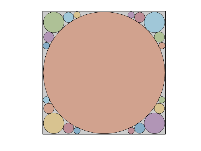
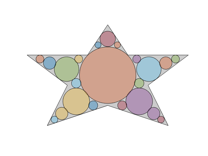
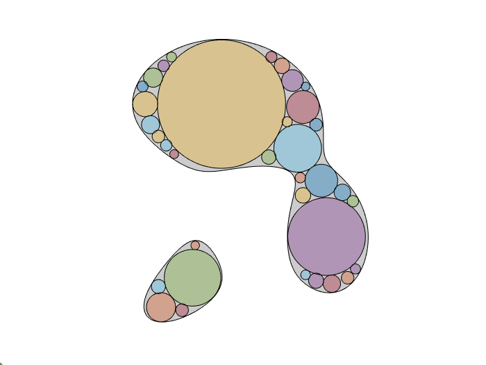
Figure 2: Three obstacles approximated by disjoint circles.

Note that this step is process, as described is somewhat computationally burdensome, but it is done in preprocessing. As an alternative, if one wishes to do this in real time (and possibly do away with the need to approximate the obstacle by circles), one could one may be able to embed the algorthms from [42, 43] into algorithm 1, since they also compute the distance function based on Hopf-Lax type formulas. For our purposes, we use the algorithm described above and approximate obstacles with circles.

As one final note, we point out how adding the obstacle function $O(x,t)$ to the Hamilton-Jacobi equation as in (40) affects the update rules in each of the cases above. When replacing the Hamiltonian $H(x,p)$ with $O(x_{s},t)H(x,p)$, where $x_{s}$ denotes the spatial variables in $x$, the update rules for any of the costate variables do not change in any significant way: the indicator function of the obstacles is simply brought along as a multiplier and appears anywhere where $\delta\sigma$ appears. For example, the update rules for the car given by (26) and (27) become

$$(p_{1:2})_{j}^{k+1} =\left[\max\left\{0,1-\frac{O((x_{1:2})^{k}_{j},t_{j})\delta\sigma}{\left\lvert\gamma^{T}\beta_{1:2}\right\rvert}\right\}-1\right](\gamma^{T}\beta_{1:2})\gamma+\beta_{1:2},$$

$$(p_{3})_{j}^{k+1} =\max\left\{0,1-\frac{O((x_{1:2})^{k}_{j},t_{j})\delta\sigma W}{\left\lvert\beta_{3}\right\rvert}\right\}\beta_{3},$$

which are the exact same as before aside from the inclusion of $O(x_{s},t)$ evaluated at the current spatial coordinates $(x_{1:2})^{k}_{j}$ and time step $t_{j}$. The updates for the airplane or submarine are modified in analogous ways.

Likewise, because the obstacle function $O(x_{s},t)$ depends only on the spatial variables in the state vector, the updates for the angular variables (described by equations (30), (31) for the car, by equations (33), (34) for the airplane, and by equations (38), (39) for the submarine) remain virtually unchanged, except once again for the inclusion of the obstacle function as a multiplier wherever $\delta\tau$ appears. For example, for the car, we simply need to change the function $h$ in (31) to

$$h(\theta) =-\delta\tau O((x_{1:2})^{k}_{j},t_{j})|(p_{1})^{k+1}_{j}\cos(\theta)+(p_{2})^{k+1}_{j}\sin(\theta)|$$

$$\hskip 42.67912pt+\frac{1}{2}\big{(}\theta-((x_{3})^{k}_{j}-\tau((p_{3})^{k+1}_{j}-(p_{3})^{k+1}_{j+1}))\big{)}^{2},$$

which is the exact same as before aside from the inclusion of $O(x_{s},t)$. Analogous modifications are made for the plane and submarine.

The significant change comes in the updates of the spatial components which are given for the car, airplane, and submarine by equations (29),(32), and (37) respectively. The minimization problems for these updates can no longer be resolved analytically, so they approximate the solutions using gradient descent, as was done with the angular variables before. In each case, we need to resolve

$$(x_{s})^{k+1}_{j}=\operatorname*{arg\,min}_{\overline{x}}\left\{-\delta\tau O(\overline{x}_{s},t)H(x_{a},p)+\frac{1}{2}\|\overline{x}-\nu\|^{2}\right\}$$

where $\nu=(x_{s})^{k}_{j}-\tau((p_{s})^{k+1}_{j}-(p_{s})^{k+1}_{j+1})$. To reiterate, here we are using $x_{s}$ to denote the spatial variables of $x$ (and $p_{s}$ to denote the corresponding co-state variables), and we introduce $x_{a}$ to denote the angular variables. Note that in our three models above, the Hamiltonian depends only on the angular variables $x_{a}$. To approximate the solution of the minimization problem, we use the gradient descent

$$x_{s}^{*}=x_{s}^{*}-\eta\nabla h(x_{s}^{*})$$

where $h$ is defined

$$h(x_{s})=-\delta\tau O(x_{s},t_{j})H((x_{a})^{k}_{j},p^{k+1}_{j})+\frac{1}{2}\|x_{s}-\nu\|^{2}$$

and then set $(x_{s})^{k+1}_{j}=x_{s}^{*}.$ In doing this, we will need to evaluate $\nabla O(\cdot,t)$. Recall, this function is the indicator function of the free space, which is discontinuous across the boundary of the obstacles. Accordingly, we approximate the indicator function of the free space by

$$O(x_{s},t)\approx\frac{1}{2}+\frac{1}{2}\tanh(-100d(x_{s},t))$$

where $d(x_{s},t)$ is the signed distance function to the boundary of the obstacles at time $t$ (positive inside the obstacles). This definition gives a smooth function which is approximately zero inside the obstacles and approximately 1 in the free space. Here the $100$ in the definition is an arbitrary large number. Recall, we can quickly evaluate the distance function when we are approximating the obstacles by disjoint circles. This also gives an efficient method for computing the gradient of the distance function when $x_{s}$ is outside the obstacles: it is the unit vector pointing from $x_{s}$ to the center $x_{\ell}(t)$ of nearest ball to $x_{s}$ in the collection of balls which approximates the obstacles.

Note that the updates for $x^{k+1}_{0}$—which are given by equation (28) for all three models—do not change because the Hamiltonian does not appear in these updates.

4 Simulations & Discussion

In this section, we present the results of several simulations which demonstrate the efficacy of our models. In all simulations, we choose somewhat arbitrary and synthetic data, which we list for the individual simulations. The simulations were performed on a laptop computer with an Intel(R) Core(TM) i7-10510U processor running at 1.80GHz. Besides anything described above, no further efforts were made to optimize the algorithms, though certain parts are parallelizable, and the resolution of the minimizers used to update the state variables could likely be done more efficiently. Even so, our algorithms are quite efficient as reported below.

In all cases we fix the time step $\delta=0.1$ and discretize the paths into $N=t/\delta$ steps, where $t$ is the time chosen for the simulation as seen in algorithm 1. Whenever it is necessary to use gradient descent to perform the updates described in sections 3.1-3.3, we perform 3 steps of gradient descent with a descent rate of $\eta=0.03$. In each case, we continue the iteration until the maximum change in any coordinate of $x$ or $p$ is less than $\text{TOL}=10^{-3}$. This tolerance may appear fairly large, but there was no appreciable difference in the resolved optimal trajectories when this tolerance was decreased to $10^{-8}$, and the latter setting required considerably more clock time to finish the iteration and would sometimes hit the maximum iteration count of $K=100000$.

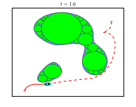
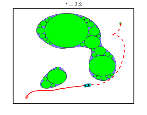
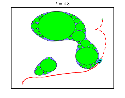
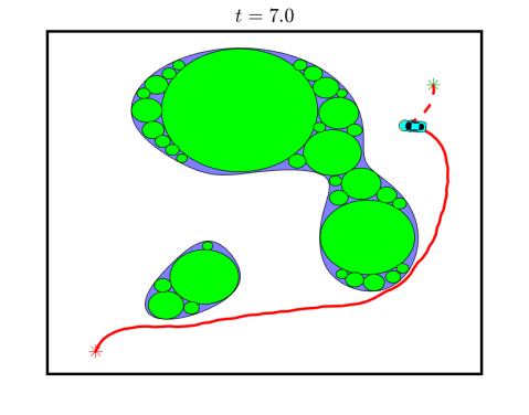
Figure 3: A car navigating around obstacles to end point in the top right of each frame. The obstacles are the blue regions, and the collection of green circles is their computational representation.

Our first two simulations, the results of which are shown in figure 3 and figure 4, show a car beginning in the configuration $(x_{0},y_{0},\theta_{0})=(-1.5,1.5,\pi/2)$ and navigating around obstacles to the point $(x_{f},y_{f},\theta_{f})=(2,2,3\pi/2)$ which are in the bottom-left and top-right (respectively) of the domain used to plot the results. In both cases, the maximum angular velocity is $W=2$. The obstacles in both figures have the same shape, but in figure 3 the obstacles remain stationary, whereas in figure 4, the obstacles rotation clockwise around the origin at a constant rate of 1 radian per unit time. In the former figure, the time required to reach the endpoint is $T=8$, whereas, when the obstacles rotate out of the way in the latter figure, the car can reach the endpoint by time $T=6$.

As mentioned in section 2.4, the time-horizon $T$ that is chosen for the problem does actually matter here. Theoretically, for any $T$ chosen large enough, there is an optimal path from the initial point to the end point. However, empirically if $T$ is chosen too large the algorithm will require longer to converge. As chosen for each of these simulations, the time horizons of $T=8$ and $T=6$, respectively, are very close to the best possible travel time, and the algorithm was able to resolve optimal paths in roughly 2.5 seconds using on the order of 1500 iterations (though there is some randomness due to initialization, these remained fairly stable). If $T$ is chosen too small, so that no path requiring time less than $T$ to traverse can reach the endpoint, then the algorithm will often fail to converge, or converge to a path which is not meaningful. If $T$ is chosen too large, then any path which reaches the endpoint is an optimal path. In this case, the car will usually dawdle for a bit, wasting some time before arriving at the endpoint at the time horizon $T$. Paths like this are likely not the optimal path one would wish to resolve, though in may case, one could easily intuit the “correct” optimal path from on of these paths. The larger issue is that this slows down convergence of the algorithm. In this example, if we run the same simulation from figure 4

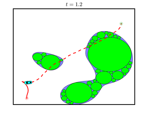
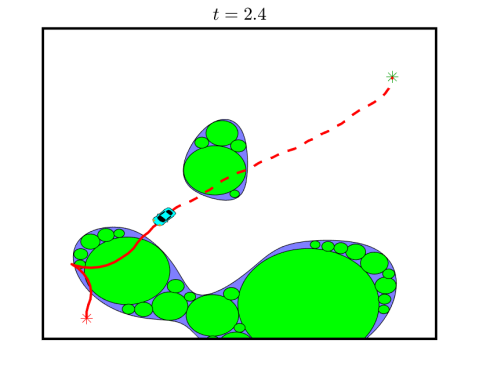
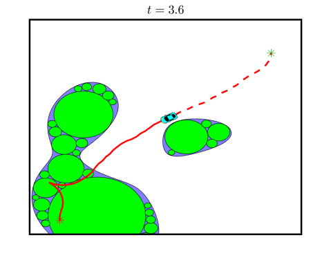
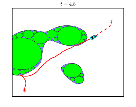
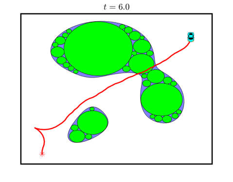
Figure 4: A car navigating around the same obstacles as in figure 4, but in this case the obstacles begin rotating clockwise about the center of the domain.

using $T=9$ (rather than $T=6$) as the time horizon, the algorithm requires on the order of 8 seconds to converge using on the order of roughly 4500 iterations. Note that the complexity of the algorithm should scale linearly with $T$, since the number of optimization problem solved at each iteration scales linearly with $T$. Thus it is undesirable for the clock time to increasing threefold when $T$ is scaled by 1.5, but this is accounted for by the additional iterations that are required for convergence. One final note is that, in these examples if the tolerance for convergence is decreased to $\text{TOL}=10^{-6}$, the optimal trajectories do not appreciably change, but the clock time increases to roughly 20 seconds, requiring on the order of 10000-15000 iterations for convergence.

Our next simulation has a Dubins airplane circling down for a landing, which is displayed in figure 5. The airplane begins in the configuration $(x_{0},y_{0},z_{0},\theta_{0})=(0,0,\tfrac{1}{2},0)$ and must end at $(x_{f},y_{f},z_{f},\theta_{f})=(0,0,0,0).$ In this case, the maximum angular velocity in the $xy$-plane is $W_{xy}=2.5$ and the maximum angular velocity in the $z$-direction is $W_{z}=0.5$. In order to make its descent, the airplane flies in a perfect figure eight in the $xy$-plane, while descending in the $z$-direction. In figure 5, the 3D view is displayed on the left of each panel and the projection down to the $xy$-plane is displayed on the right of each panel. This simulation required on the order of 2 seconds of clock time to resolve the optimal path, doing so in roughly 7000 iterations. The updates for the plane are a bit simpler than those for the car (since the plane can only move forward) which explains why more iterations can be performed in a similar clock time. For this example, if tolerance for convergence is decreased to $\text{TOL}=10^{-6}$, there is once again no appreciable difference in the trajectories generated, though the iteration count often hits the upper limit of 100000 iterations before converging.

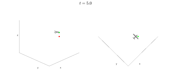
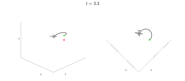
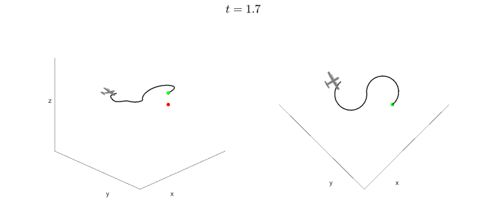
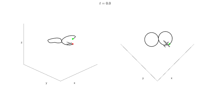
Figure 5: A Dubins airplane circling down for a landing. The 3D view is displayed on the left of each panel, and the projection down to the $xy$-axis is displayed on the right.

Finally, our last simulation has a Dubins submarine beginning at configuration $(x_{0},y_{0},z_{0},\theta_{0},\varphi_{0})=(-1.8,-1.8,0,\pi/4,\pi/2)$ and navigating through and around obstacles to $(x_{f},y_{f},z_{f},\theta_{f},\varphi_{f})=(1.3,1.5,-1.5,0,\pi/2).$ In this case, the maximum angular velocity is $W=2$. The result is displayed in figure 6, where the “third person” view is displayed on the left of each panel and the corresponding “first person” view is displayed on the right. In figure 6, the red bubbles are obstacles. This simulation (and comparable simulations for this vehicle) required roughly 12 seconds of clock time to resolve the optimal trajectory in roughly 4000 iterations. Here the iterations are more expensive due to the resolution of $p_{4:5}$ by the bisection method described in equations (35), (36). Once again, if we decrease the convergence tolerance to $\text{TOL}=10^{-6}$, the path generated is not appreciably different, but requires roughly 1 minute of clock time and on the order of 20000 iterations to resolve.

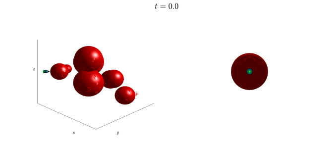
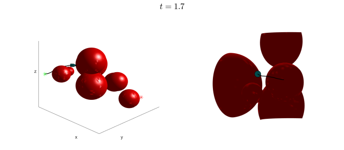
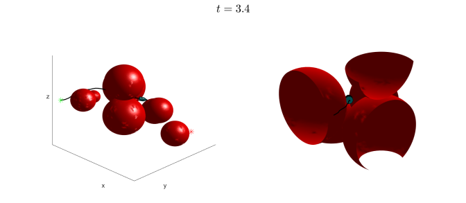
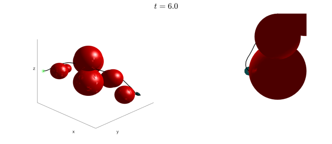
Figure 6: A Dubins submarine navigating through and around obstacles to reach its desired destination. The “third-person” view is displayed on the left of each panel, while the corresponding “first-person” view is displayed on the right. The red bubbles are obstacles.

5 Conclusion & Future Work

In this paper, we developed an algorithm for optimal path-planning for curvature constrained motion which includes kinematic models for simple cars, airplanes, and submarines. Our method relied on a level-set, PDE-based formulation of the optimal path-planning problem, wherein the value function is not the optimal travel time (as in more control theoretic models), but optimal distance to the desired endpoint. This allowed us to solve the problem using new numerical methods which resolve the solutions to Hamilton-Jacobi equations via optimization problems. We discussed the ramifications of this modeling decision, and described in detail the implementation of our method. Finally, we demonstrated our method on some synthetic examples. In these examples, we are able to resolve optimal trajectories for cars, planes, and submarines in a matter of seconds. This allows one to maintain the PDE and control based methodology (and thus maintain interpretability) without sacrificing efficiency.

While this represents a step toward real-time PDE-based path-planning algorithms, there are still difficulties to overcome. As presented, our method can compute optimal paths in a fully-known environment. In realistic scenarios, the exact configuration of obstacles is likely unknown and obstacles may move unpredictably. Accordingly, we would like to integrate our planning method with environment discovery algorithms so that the vehicles could react and recompute paths in semi-real-time. In doing so, one would need to abandon the hope of finding globally optimal trajectories, because only local information would be known. In the same vein, it could prove interesting to adapt and apply our method to problems with other realistic concerns such as energy-efficient path-planning. Finally, we would like to adapt this method to a multi-agent control or many-player differential game scenario.

References

- [1] L. E. Dubins, On curves of minimal length with a constraint on average curvature, and with prescribed initial and terminal positions and tangents, American Journal of mathematics 79 (3) (1957) 497–516.
- [2] J. Reeds, L. Shepp, Optimal paths for a car that goes both forwards and backwards, Pacific journal of mathematics 145 (2) (1990) 367–393.
- [3] J. Barraquand, J.-C. Latombe, Nonholonomic multibody mobile robots: Controllability and motion planning in the presence of obstacles, Algorithmica 10 (2-4) (1993) 121.
- [4] P. K. Agarwal, H. Wang, Approximation algorithms for curvature-constrained shortest paths, SIAM Journal on Computing 30 (6) (2001) 1739–1772.
- [5] R. Takei, R. Tsai, H. Shen, Y. Landa, A practical path-planning algorithm for a simple car: a Hamilton-Jacobi approach, in: Proceedings of the 2010 American Control Conference, 2010, pp. 6175–6180.
- [6] R. Takei, R. Tsai, Optimal trajectories of curvature constrained motion in the Hamilton-Jacobi formulation, Journal of Scientific Computing 54 (2) (2013) 622–644.
- [7] D. J. Arnold, D. Fernandez, R. Jia, C. Parkinson, D. Tonne, Y. Yaniv, A. L. Bertozzi, S. J. Osher, Modeling environmental crime in protected areas using the level set method, SIAM Journal on Applied Mathematics 79 (3) (2019) 802–821.
- [8] C. Parkinson, D. Arnold, A. L. Bertozzi, Y. T. Chow, S. Osher, Optimal human navigation in steep terrain: a hamilton–jacobi–bellman approach, Communications in Mathematical Sciences 17 (1) (2019) 227–242.
- [9] C. Parkinson, D. Arnold, A. Bertozzi, S. Osher, A model for optimal human navigation with stochastic effects, SIAM Journal on Applied Mathematics 80 (4) (2020) 1862–1881.
- [10] C. Parkinson, A. L. Bertozzi, S. J. Osher, A hamilton-jacobi formulation for time-optimal paths of rectangular nonholonomic vehicles, in: 2020 59th IEEE Conference on Decision and Control (CDC), IEEE, 2020, pp. 4073–4078.
- [11] C. Parkinson, M. Ceccia, Time-optimal paths for simple cars with moving obstacles in the hamilton-jacobi formulation, in: 2022 American Control Conference (ACC), IEEE, 2022, pp. 2944–2949.
- [12] B. Chen, K. Peng, C. Parkinson, A. L. Bertozzi, T. L. Slough, J. Urpelainen, Modeling illegal logging in brazil, Research in the Mathematical Sciences 8 (2) (2021) 1–21.
- [13] M. Gee, A. Vladimirsky, Optimal path-planning with random breakdowns, IEEE Control Systems Letters 6 (2021) 1658–1663.
- [14] E. Cartee, L. Lai, Q. Song, A. Vladimirsky, Time-dependent surveillance-evasion games, in: 2019 IEEE 58th Conference on Decision and Control (CDC), IEEE, 2019, pp. 7128–7133.
- [15] A. Shukla, E. Singla, P. Wahi, B. Dasgupta, A direct variational method for planning monotonically optimal paths for redundant manipulators in constrained workspaces, Robotics and Autonomous Systems 61 (2) (2013) 209–220.
-
[16]
F. Zhang, C. Wang, C. Cheng, D. Yang, G. Pan,
Reinforcement learning path
planning method with error estimation, Energies 15 (1) (2022).
URL https://www.mdpi.com/1996-1073/15/1/247 - [17] K. Wan, D. Wu, B. Li, X. Gao, Z. Hu, D. Chen, Me-maddpg: An efficient learning-based motion planning method for multiple agents in complex environments, International Journal of Intelligent Systems 37 (3) (2022) 2393–2427.
- [18] R. Deng, Q. Zhang, R. Gao, M. Li, P. Liang, X. Gao, A trajectory tracking control algorithm of nonholonomic wheeled mobile robot, in: 2021 6th IEEE International Conference on Advanced Robotics and Mechatronics (ICARM), 2021, pp. 823–828.
- [19] J. J. Johnson, M. C. Yip, Chance-constrained motion planning using modeled distance- to-collision functions, in: 2021 IEEE 17th International Conference on Automation Science and Engineering (CASE), 2021, pp. 1582–1589.
- [20] J. Darbon, S. Osher, Algorithms for overcoming the curse of dimensionality for certain hamilton–jacobi equations arising in control theory and elsewhere, Research in the Mathematical Sciences 3 (1) (2016) 19.
- [21] Y. T. Chow, J. Darbon, S. Osher, W. Yin, Algorithm for overcoming the curse of dimensionality for state-dependent hamilton-jacobi equations, Journal of Computational Physics 387 (2019) 376–409.
- [22] A. T. Lin, Y. T. Chow, S. J. Osher, A splitting method for overcoming the curse of dimensionality in Hamilton–Jacobi equations arising from nonlinear optimal control and differential games with applications to trajectory generation, Communications in Mathematical Sciences 16 (7) (1 2018).
- [23] S. Osher, J. A. Sethian, Fronts propagating with curvature-dependent speed: Algorithms based on hamilton-jacobi formulations, Journal of computational physics 79 (1) (1988) 12–49.
- [24] F. Gibou, R. Fedkiw, S. Osher, A review of level-set methods and some recent applications, Journal of Computational Physics 353 (2018) 82–109.
- [25] R. Bellman, Dynamic programming, Science 153 (3731) (1966) 34–37.
- [26] M. G. Crandall, P.-L. Lions, Viscosity solutions of hamilton-jacobi equations, Transactions of the American mathematical society 277 (1) (1983) 1–42.
- [27] M. G. Crandall, H. Ishii, P.-L. Lions, User’s guide to viscosity solutions of second order partial differential equations, Bulletin of the American mathematical society 27 (1) (1992) 1–67.
- [28] M. Bardi, I. C. Dolcetta, et al., Optimal control and viscosity solutions of Hamilton-Jacobi-Bellman equations, Vol. 12, Springer, 1997.
- [29] S. Jafarpour, On small-time local controllability, SIAM Journal on Control and Optimization 58 (1) (2020) 425–446.
- [30] C. Parkinson, A rotating-grid upwind fast sweeping scheme for a class of hamilton-jacobi equations, Journal of Scientific Computing 88 (1) (2021) 13.
- [31] C.-Y. Kao, S. Osher, Y.-H. Tsai, Fast sweeping methods for static hamilton–jacobi equations, SIAM journal on numerical analysis 42 (6) (2005) 2612–2632.
- [32] Y.-T. Zhang, H.-K. Zhao, J. Qian, High order fast sweeping methods for static hamilton–jacobi equations, Journal of Scientific Computing 29 (2006) 25–56.
- [33] J. N. Tsitsiklis, Efficient algorithms for globally optimal trajectories, IEEE transactions on Automatic Control 40 (9) (1995) 1528–1538.
- [34] J. A. Sethian, Fast marching methods, SIAM review 41 (2) (1999) 199–235.
- [35] K. Alton, I. M. Mitchell, Fast marching methods for stationary hamilton–jacobi equations with axis-aligned anisotropy, SIAM Journal on Numerical Analysis 47 (1) (2009) 363–385.
- [36] J. A. Sethian, A. Vladimirsky, Ordered upwind methods for static hamilton–jacobi equations: Theory and algorithms, SIAM Journal on Numerical Analysis 41 (1) (2003) 325–363.
- [37] A. Chambolle, T. Pock, A first-order primal-dual algorithm for convex problems with applications to imaging, Journal of mathematical imaging and vision 40 (2011) 120–145.
- [38] M. Zhu, T. Chan, An efficient primal-dual hybrid gradient algorithm for total variation image restoration, Ucla Cam Report 34 (2008) 8–34.
- [39] E. Esser, X. Zhang, T. F. Chan, A general framework for a class of first order primal-dual algorithms for convex optimization in imaging science, SIAM Journal on Imaging Sciences 3 (4) (2010) 1015–1046.
- [40] S. Osher, R. P. Fedkiw, Level set methods and dynamic implicit surfaces, Vol. 1, Springer New York, 2005.
- [41] J. A. Sethian, Level set methods and fast marching methods: evolving interfaces in computational geometry, fluid mechanics, computer vision, and materials science, Vol. 3, Cambridge university press, 1999.
- [42] B. Lee, J. Darbon, S. Osher, M. Kang, Revisiting the redistancing problem using the hopf–lax formula, Journal of Computational Physics 330 (2017) 268–281.
- [43] M. Royston, A. Pradhana, B. Lee, Y. T. Chow, W. Yin, J. Teran, S. Osher, Parallel redistancing using the hopf–lax formula, Journal of Computational Physics 365 (2018) 7–17.