Median of heaps: linear-time selection by recursively constructing binary heaps

Abstract

The first worst-case linear-time algorithm for selection was discovered in 1973; however, linear-time binary heap construction was first published in 1964. Here we describe another worst-case linear selection algorithm, which is simply implemented and uses binary heap construction as its principal engine. The algorithm is implemented in place, and shown to perform similarly to in-place median of medians.

1 Introduction

Selection is the problem of finding the $\tau^{*}=k^{\text{th}}$ smallest value in a collection. Online versions of this problem exist, but or simplicity, here we focus on selecting from a list $x_{1},x_{2},\ldots,x_{n}$. Selection can be trivially performed via sorting in $O(n\log(n))$ to retrieve $\tau^{*}$. Selection can also be performed by popping values from a heap or priority queue in $O(n+k\log(n))$[1]; however, computing the median (i.e., $k=\frac{n}{2}$) requires $O(n\log(n))$ steps.

Hoare’s quickselect, published in 1961 algorithm was the first algorithm with a runtime practically faster than sorting $\forall k$.[2] It was published concurrently with Hoare’s quicksort algorithm and operates in a similar manner[3]: Quickselect chooses a random element $\tau=x_{i}$ and “pivots” by partitioning the array in $O(n)$ into values $<\tau$ and values $\geq\tau$. In doing so, the rank of $\tau$, $r(x,\tau)=|\{j:x_{j}<\tau\}|$ is counted. When $k<r(x,\tau)$, recursive selection is continued on the smaller values. Likewise, when $k>r(x,\tau)$, recursion is continued on the larger values. And if $k=r(x,\tau)$, $\tau=\tau^{*}$.

While quickselect, like quicksort, can be seen to have an expected runtime in $O(n\log(n))$ via a harmonic series[4], its worst-case runtime remains in $\Omega(n^{2})$. This can occur when $\tau\in\{min(x),max(x)\}$, or more generally, $r(x,\tau)\in O(1)\wedge n-r(x,\tau)\in O(1)$ and thus $\Theta(n)$ is spent to partition when only eliminating $O(1)$ elements.

In 1973, Blum et al. discovered that selection could be performed in worst-case $O(n)$ time[5]. Blum et al.’s “median of medians” algorithm operates by grouping $x$ into subgroups of length $5$. The median of each group of 5 is computed in $O(1)$, for $O(n)$ steps over all groups of 5. The algorithm then recurses to compute the median of these $\frac{n}{5}$ medians. This median of medians value, $\tau$, is used for partitioning $x$ in the same manner as quickselect; however, the median of medians is proveably a middle element, where both $r(x,\tau)$ and $n-r(x,\tau)$ are provably large. This guarantees that when $\tau\neq\tau^{*}$, the recursion on either the larger or smaller elements would consider only a fraction of $n$. Specifically, $r(x,\tau),n-r(x,\tau)\geq\frac{3n}{10}$, because each group of 5 where the median of the group is $<\tau$ has 3 values $<\tau$, and there are $\approx\frac{n}{2}$ such groups. The resulting recurrence is $T(n)=T\left(\frac{n}{5}\right)+T\left(\frac{7n}{10}\right)+O(n)$. Together, the recursion to compute the median of medians and the recursion to select the remainder consider at most $\frac{9n}{10}$. This results in a root-heavy case of the master theorem, wherein regularity guarantees $T(n)\in\Theta(n)$. Median of medians is regarded as a groundbreaking algorithm for its approach.

In subsequent years, alternate algorithms have been discovered, which select by traversing values in a heaps or by using approximate priority queues. These algorithms are more sophisticated and complicated to implement[6, 7].

Since 1964, it was known that construction of a binary heap (“heapifying”) can be performed by heapifying both the left and right $\frac{n}{2}$ and then melding those heaps by reheaping in $O(\log(n))$ operations[1]. The resulting recurrence $T(n)=2\cdot T\left(\frac{n}{2}\right)+\log(n)$ is a leaf-heavy case of the master theorem, with $T(n)\in\Theta(n)$.

Here we introduce a fairly simple in-place and worst-case $O(n)$ selection algorithm, which follows directly from construction of a binary heap itself. A partition element $\tau:r(x,\tau),n-r(x,\tau)\geq c\cdot n$ for constant $c>0$ can be trivially discovered by recursively heapifying one level of each heap tree and recursing downward.

2 Methods

2.1 Basic procedure

The algorithm proceeds as follows:

First, heapify $x$ in an array, where $x_{i}<x_{2i+1},x_{2i+2}$. Levels of the tree are contiguous in memory: level $i$ has $2^{i}$ values, $y_{i}=x_{2^{i}},x_{2^{i}+1},\ldots,x_{2^{i+1}}-1$.

The heap is a complete tree. Let $d$ be the depth at which the heap is perfect, $d=\lfloor\log_{2}(n+1)-1\rfloor$. Let $\ell$ be the level of the tree where $\tau$ is found via recursive selection. Let that recursive selection $\tau=select(y_{\ell},k^{\prime})$ partitions $y_{\ell}$ via $\tau$ where $r(y_{\ell},\tau)=k^{\prime}-1$ elements in $y_{\ell}$ are $<\tau$ and $2^{\ell}-k^{\prime}$ values are $\geq\tau$ (excluding the element corresponding to $\tau$ itself).

By choosing level $\ell<d$ and by choosing $k^{\prime}$ to select somewhere from the middle of $y_{\ell}$, inequalities can be stacked. This is portrayed by chains in the digraph visualized by Figure 1: $y_{\ell}$ contains 1 value $<\tau$ and 2 values $\geq\tau$, but the 2 ancestors of all values $<\tau$ are likewise $<\tau$. Similarly, the 7 descendents of values $\geq\tau$ are $\geq\tau$.

Figure 1: Illustration of stacked inequalities after selection on level $y_{2}$ of the heap tree. A level toward the bottom of the tree, $y_{2}$, is recursively partitioned via selection to find $\tau$. The directed edge $a\rightarrow b$ depicts inequality $a<b$. Choosing a middle level in the tree results in stacked inequalities, represented here as chains of directed edges. This figure depicts $n=20$ values, $d=3$ deepest perfect layer, $t=5$ remaining values in the final imperfect layer, and the $k^{\prime}=1$ value recursively selected from $y_{2}$.

2.2 Optimization of $k^{\prime}$

We will optimize both $k^{\prime}$ and later the level $\ell$ from which it is selected.

The $k^{\prime}-1$ values in $y_{\ell}$ that are $<\tau$ imply at least $k^{\prime}-1+\frac{k^{\prime}-1}{2}+\frac{k^{\prime}-1}{4}+\cdots+2+1=2k^{\prime}-3$ values $<\tau$ (including the $k^{\prime}+1$ nodes and their ancestors). The $2^{\ell}-k^{\prime}$ values $\geq\tau$ imply at least $(2^{\ell}-k^{\prime})\cdot(2^{d-\ell+1}-1)$ values $\geq\tau$.

We can balance the number of values $<\tau$ and $\geq\tau$ by allowing $2k^{\prime}-3=(2^{\ell}-k^{\prime})\cdot(2^{d-\ell+1}-1)$, which yields

$$k^{\prime} = \frac{2^{d+1}-2^{\ell}+3}{2^{d-\ell+1}+1}$$

$$\approx \frac{2^{d-\ell+1}-1}{2^{d-\ell+1}+1}\cdot 2^{\ell}$$

Because we’ve balanced the number of values provably $<\tau$ and $\geq\tau$, at least $\approx 2k^{\prime}$ values will be excluded. Hence, the proportion of $x$ excluded will be $\approx\frac{2k^{\prime}}{n}$.

The worst-case runtime is characterized by

$$T(n) = T\left(2^{\ell}\right)+T\left(\left(1-\frac{2k^{\prime}}{n}\right)\cdot n\right)+\Theta(n)$$

$$= T\left(\frac{2^{\ell}}{n}\cdot n\right)+T\left(\left(1-\frac{2k^{\prime}}{n}\right)\cdot n\right)+\Theta(n).$$

Thus, regularity requires

$$c = \frac{2^{\ell}}{n}+1-\frac{2k^{\prime}}{n}$$

$$= 1+\frac{2^{\ell}-2k^{\prime}}{n}$$

$$= 1+2^{\ell}\cdot\frac{1-2\cdot\frac{2^{d-\ell+1}-1}{2^{d-\ell+1}+1}}{n}<1.$$

2.2.1 Case 1: perfect heap

When the heap is perfect, $n=2^{d+1}-1$; therefore,

$$c_{\text{perfect}}\approx 1+2^{\ell-d-1}\cdot\left(1-2\cdot\frac{2^{d-\ell+1}-1}{2^{d-\ell+1}+1}\right).$$

2.2.2 Case 2: imperfect heap

When the heap is imperfect, $n\in\left(2^{d+1}-1,2\cdot(2^{d+1}-1)\right)\approx\left(2^{d+1},2^{d+2}\right).$ Thus,

$$c_{\text{imperfect}}\approx 1+\lambda\cdot 2^{\ell-d-1}\cdot\left(1-2\cdot\frac{2^{d-\ell+1}-1}{2^{d-\ell+1}+1}\right),$$

where $\lambda\in\left(\frac{1}{2},1\right)$.

Assuming regularity in case 1, the worst-case $c_{\text{imperfect}}$ will occur at $\lambda=\frac{1}{2}$, because $c_{\text{perfect}}$ decreases from 1, where minimizing $\lambda$ will minimize this decrease from 1. First, this proves that regularity in case 1 implies regularity in case 2, and would thus imply $T(n)\in\Theta(n)$. Second, it yields the worst-case $c$ for imperfect heaps:

$$c_{\text{imperfect}}\approx 1+2^{\ell-d-2}\cdot\left(1-2\cdot\frac{2^{d-\ell+1}-1}{2^{d-\ell+1}+1}\right).$$

2.2.3 Case 3: revising the algorithm to tighten the worst-case bound on imperfect trees

The runtime bound above for imperfect heaps is conservative.

Let $t=n-2^{d+1}-1\geq 0$ be the number of nodes in the final, imperfect level of the heap if the tree. When the tree is perfect, $t=0$. At worst, $k^{\prime}\cdot(2^{d-\ell+1}-1)$ of the $t$ values in the imperfect level will have non-stacking inequalities. I.e., at worst, these values’ ancestors in $y_{\ell}$ are $<\tau$, but the values are $\geq$ their ancestors, leaving non-stacking inequalities. The remaining at least $t-k^{\prime}\cdot(2^{d-\ell+1}-1)$ values that must be $\geq\tau$. Thus, we could achieve tighter bounds by solving

$$2k^{\prime} \approx (2^{\ell}-k^{\prime})\cdot(2^{d-\ell+1}-1)+t-k^{\prime}\cdot(2^{d-\ell+1}-1)$$

$$\leftrightarrow k^{\prime} \approx \frac{2^{d+1}+t-2^{\ell}}{2^{d-\ell+2}}$$

$$\approx \frac{n-2^{\ell}}{2^{d-\ell+2}}.$$

Once again, let $\lambda\approx\frac{2^{d+1}}{n}\in\left[\frac{1}{2},\lambda_{\max}\right)$, where $\lambda_{\max}<1$ is determined by $t-k^{\prime}\cdot(2^{d-\ell+1}-1)=0$.

$$c = 1+\frac{2^{\ell}-2k^{\prime}}{n}$$

$$= 1+\frac{2^{\ell}}{n}-2\cdot\frac{1-\frac{2^{\ell}}{n}}{2^{d-\ell+2}}.$$

$\frac{2^{\ell}}{n}=\lambda\cdot 2^{\ell-d-1}$; therefore, denoting $a=2^{\ell-d-1}\in(0,1)$, we have

$$c = 1+\lambda\cdot a-2\cdot\frac{1-\lambda\cdot a}{\frac{2}{a}}$$

$$= 1+\lambda\cdot a-a+\lambda\cdot a^{2}$$

$$= 1+a\cdot(\lambda\cdot(1+a)-1).$$

$\frac{\partial c}{\partial\lambda}\neq 0$, so the worst-case $\lambda$ occurs at a boundary $\lambda=\lambda_{\max}$. Thus we see that the worst-case scenario is achieved by $t-k^{\prime}\cdot(2^{d-\ell+1}-1)=0$.

When this occurs, we choose $k^{\prime}$ as in cases 1 & 2. In bounding $c$, what changes is

$$\frac{2^{\ell}}{n} = \frac{2^{\ell}}{2^{d+1}-1+t}$$

$$\approx \frac{2^{\ell}}{2^{d+1}+t}$$

$$= \frac{2^{\ell}}{2^{d+1}+k^{\prime}\cdot(2^{d-\ell+1}-1)}$$

$$\rightarrow c = 1+2^{\ell}\cdot\frac{1-2\cdot\frac{2^{d-\ell+1}-1}{2^{d-\ell+1}+1}}{2^{d+1}+k^{\prime}\cdot(2^{d-\ell+1}-1)}$$

$$= 1+2^{\ell}\cdot\frac{1-2\cdot\frac{2^{d-\ell+1}-1}{2^{d-\ell+1}+1}}{2^{d+1}+k^{\prime}\cdot(2^{d-\ell+1}-1)}$$

$$= 1+\frac{1-2\cdot\frac{2^{d-\ell+1}-1}{2^{d-\ell+1}+1}}{2^{d-\ell+1}+\frac{k^{\prime}}{2^{\ell}}\cdot(2^{d-\ell+1}-1)}$$

$$= 1+\frac{1-2\cdot\frac{2^{d-\ell+1}-1}{2^{d-\ell+1}+1}}{2^{d-\ell+1}+\frac{2^{d-\ell+1}-1}{2^{d-\ell+1}+1}\cdot(2^{d-\ell+1}-1)}.$$

Listing 3 implements this revised algorithm.

2.2.4 Optimizing $\ell$ to minimize worst-case $c$

Table 1 shows the relationship between $\ell$ and $c$ for perfect and imperfect heaps. The best asymptotic worst-case runtime (corroborated analytically, not shown) is given by $\ell=d-2$. For the basic median of heaps, $k^{\prime}=\frac{7}{9}\cdot 2^{\ell}$, achieving $c<1$. This generalizes the runtime bound to prove $T(n)\in\Theta(n)$ for the basic median of heaps algorithm for both perfect and imperfect heaps.

The revised algorithm yields a tighter bound on $c$ for imperfect heaps. Note that although both the basic and revised algorithms behave identically on the first recursion when $n=2^{i}-1$ (i.e., a perfect heap), the recursion after partitioning is no longer guaranteed to be perfect. Thus, the worst-case constant of geometric decay will be determined by $c_{\text{imperfect}}$.

$d-\ell$	$c_{\text{perfect}}$	$c_{\text{imperfect}}$ (basic alg.)	$c_{\text{imperfect}}$ (revised alg.)
0	1.1667	1.0833	1.1429
1	0.9500	0.9750	0.9655
2	0.9306	0.9653	0.9587
3	0.9522	0.9761	0.9738
4	0.9725	0.9863	0.9856
5	0.9853	0.9927	0.9925

Table 1: Relationship between $\ell$ and $c$. For $k^{\prime}$ chosen as described, the worst-case constant of geometric decay for the median of heaps algorithm is shown for perfect heaps. Also shown are the worst-case gemoetric decay constants for the basic and revised median of heaps algorithms on imperfect heaps. In all cases, the greatest decay in the worst case is found $\ell=d-2$. Values are rounded to ${10}^{-4}$.

2.3 Implementation

Quickselect was implemented via random pivot and std::partition.

Median of medians was implemented in place by striding by powers of 5 as recursions become deeper. Strided arrays are accessed via a class and iterators, allowing use of std::sort on each group of 5 as well as selecting with std::sort when $n<16$. When $n\not\equiv 0\text{(mod 5)}$, the remaining 4 or fewer values were excluded when computing the median of medians.

Listing 1 and Listing 2 demonstrate implementations in python and C++, respectively. Neither implementation considers $t$ when choosing $k$, deferring to the weaker bound for imperfect heaps. For expected rather than worst-case performance, the implementations use $\ell=d-1$ and thus $k^{\prime}=\frac{3}{5}\cdot 2^{\ell}$.

By changing to another selection algorithm when $n$ is a sufficiently large constant base case, we are assured the existence of level $\ell=d-1$ in the heap. Here we stop recursion when $n<16$, which at most corresponds to a perfect heap of $8+4+2+1=15$ values.

Listing 3 shows the more complicated revised median of heaps algorithm, achieving a tighter worst-case bound on $c$.

⬇

import numpy as np

from heapq import heapify

import math

def pivot(x, tau):

x = np.array(x)

return list(x[x<tau]), list(x[x>=tau])

def sel_sort(x, k):

return sorted(x)[k]

def sel_median_of_heaps(x, k):

n = len(x)

if n < 16:

return sorted(x)[k]

x = list(x)

heapify(x)

d = int(math.log2(n+1)-1)

# second-to-last perfect level in the tree:

y = x[2**(d-1)-1 : 2**(d-0)-1]

tau = sel_median_of_heaps(y, 3*len(y)//5)

x_small, x_big = pivot(x, tau)

n_small = len(x_small)

if k < n_small:

return sel_median_of_heaps(x_small, k)

return sel_median_of_heaps(x_big, k-n_small)

Listing 1: Python implementation of basic median of heaps algorithm. Using $\ell=d-1$ and thus $k^{\prime}=\frac{3}{5}\cdot 2^{\ell}$.

⬇

#include <algorithm>

#include <functional>

#include <math.h>

template <typename T>

T sel_sort(T*x, long n, long k) {

std::sort(x, x+n);

return x[k];

}

template <typename T>

T sel_median_of_heaps(T*x, long n, long k) {

if (n<16)

return sel_sort(x, n, k);

/* builds max heap, so use > as < to build a min heap: */

std::make_heap(x, x+n, std::greater<T>());

/* final perfect level in the tree: */

long d = log2(n+1) - 1;

/* second-to-last perfect level in the tree: */

long i_start = (1L<<(d-1)) - 1;

T*y = x + i_start;

long len_y = 1L<<(d-1);

long tau = sel_median_of_heaps(y, len_y, 3*len_y/5);

/* partition into the values < tau and the values >= tau: */

T*x_prime = std::partition(x, x+n, [tau](const auto & val) {

return val<tau; });

long n_small = x_prime - x;

if (k < n_small)

return sel_median_of_heaps(x, n_small, k);

return sel_median_of_heaps(x_prime, n-n_small, k-n_small);

}

Listing 2: In-place C++ implementation of median of basic heaps algorithm. Using $\ell=d-1$ and thus $k^{\prime}=\frac{3}{5}\cdot 2^{\ell}$.

⬇

template <typename T>

T sel_median_of_heaps_tight(T*x, long n, long k) {

// increased from 16 because approx has been applied sufficiently

// that bounds need a slightly larger base case.

if (n<32)

return sel_sort(x, n, k);

// makes a max heap, so use > as the < operator to build a min heap:

std::make_heap(x, x+n, std::greater<T>());

// final perfect level in the tree:

long d = log2(n+1) - 1L;

long ell = d-1L;

long len_y = 1L<<ell;

long i_start = len_y - 1L;

T*y = x + i_start;

// number of nodes in the final, imperfect layer:

long t = n - ((1L<<(d+1)) - 1L);

// solve 2k = (2**ell - k)*(2**(d-ell+1) - 1) + t - k*(2**(d-ell+1) - 1)

long k_prime = (n - len_y) / (1L<<(d-ell+2L));

if ( t - k_prime*( (1L<<(d-ell+1L)) - 1L ) < 0) {

// final, imperfect layer has few values. revert to basic version

// and solve 2k = (2**ell - k)*(2**(d-ell+1) - 1)

long fold_vs_last_full = 1L<<(d-ell+1);

k_prime = (fold_vs_last_full - 1) * len_y / (fold_vs_last_full + 1);

}

long tau = sel_median_of_heaps_tight(y, len_y, k_prime);

// partition into the values < tau and the values >= tau:

T*x_prime = std::partition(x, x+n, [tau](const auto & val) {

return val<tau;});

long n_small = x_prime - x;

if (k < n_small)

return sel_median_of_heaps_tight(x, n_small, k);

return sel_median_of_heaps_tight(x_prime, n-n_small, k-n_small);

}

Listing 3: In-place C++ implementation of median of heaps revised to tighten $c$ bound. Using $\ell=d-1$. This algorithm is shown for demonstration and is not benchmarked, because performance in practice is too similar to the simpler median of heaps variant.

3 Results

C++ runtimes were computed with $n\in\{2^{19},2^{20},\ldots,2^{32}\}$. Compilation was performed using gcc 11.3.0 and with flags -std=c++20 -O3 -march=native an Intel i9-10885H CPU at 2.40GHz and with 64GiB RAM. At each $n$, selection of the median ($k=\frac{n}{2}$) is performed via 4 algorithms: std::sort, quickselect, median of medians, and median of heaps (the simple variant, not variant with the tight bound on $c$). 5 replicate trials were timed for each $n$ and each algorithm. $x$ was filled with 64-bit random integers via (rand() << 20) ^ rand(). Random values were generated $\in\{0,1,2,\ldots,32n-1\}$. On a given replicate, each algorithm was timed using the same random seeds via srand to ensure the algorithms are compared on the same inputs. Mean, min, and max runtimes are depicted in Figure 2. Mean runtimes are reported in Table 2.

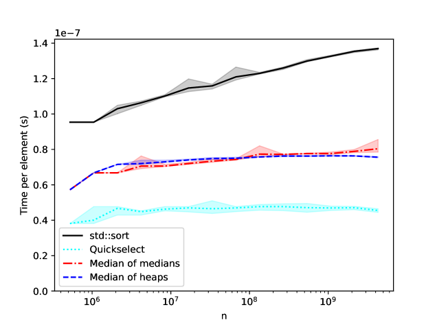
Figure 2: Per-element runtime of selection algorithms in C++. An $n$-element array is allocated, filled with random values, and the median is selected via $k=\frac{n}{2}$. Real elapsed time, including initialization of the array $x$, is recorded and aggregated over 5 replicate trials. Per-element runtimes compute the executable runtime divided by $n$. At each $n$, average runtime for an algorithm over the 5 replicates is plotted. The min and max over the 5 replicates are shaded. Note that for median of heaps, the runtime of the basic (not revised) algorithm is shown.

n	std::sort	Quickselect	Median of medians	Median of heaps (basic)
524288	0.050	0.020	0.030	0.030
1048576	0.100	0.042	0.070	0.070
2097152	0.216	0.098	0.140	0.150
4194304	0.446	0.188	0.296	0.302
8388608	0.924	0.388	0.592	0.612
16777216	1.924	0.788	1.208	1.242
33554432	3.888	1.560	2.462	2.510
67108864	8.118	3.150	4.986	5.034
134217728	16.502	6.400	10.380	10.162
268435456	33.820	12.804	20.718	20.468
536870912	69.740	25.284	41.692	40.928
1073741824	142.420	50.380	83.382	81.998
2147483648	290.772	101.070	169.420	163.908
4294967296	588.102	195.430	345.214	324.660

Table 2: Runtimes of selection algorithms in C++. Mean runtimes are rounded to $10^{-3}$ seconds, computed as described in Figure 2. Note that for median of heaps, the runtime of the basic (not revised) algorithm is shown.

4 Discussion

Figure 2 shows gap growing linearly between std::sort and the three selection algorithms benchmarked. This gap without bound for $n\gg 1$ indicates different in-practice $O(\cdot)$ runtime.

The proposed median of heaps algorithm is roughly comparable to median of medians. Both algorithms’ costs per element plateau, and are bounded above with the exception of slightly decreasing cache performance as $n\gg 1$. The more complex revised median of heaps variant performs nearly indistinguishably in practice (results not shown). It is doubtful whether the performance gain in practice justifies the additional complexity.

Both the basic and revised median of heaps algorithms here are conservative in performing comparisons: during partitioning, the algorithm partitions values whose ranks relative to $\tau$ are already known (i.e., those left and above or right and below $\tau$ in Figure 1). Proceeding out-of-place and using a buffer into which elements are copied may improve performance.

Both the median of medians and median of heaps algorithms are slower here than quickselect. This is not unexpected, as quickselect is lightweight and with low constant in expected performance.[4]

On practical performance, access is sequential during partitioning and thus cache performance is essentially optimal; however, reheaping during heapify accesses children $2i+1,2i+2$, which can be far from $i$ when $n\gg 1$, particularly during reheap propagation, when accessing parents and further ancestors does not access levels of the tree sequentially.

Similar cache penalties are incurred in the strided median of medians implementation. This could likewise be buffered, copying the medians to the buffer to recurse in-place. Buffering median of medians would have cache benefits, but would result in greater memory footprint and more copying of data.

Interestingly, the recursive calls of median of heaps unroll to many heapify operations on increasingly fine collections of values. The worst-case linear runtime implies good $\tau$ candidates can always be found in certain levels of the heap. These middle levels are enriched for these middle $\tau$ values. Other options for finding these middle $\tau$ values could be considered, thereby avoiding the recursion to compute $\tau$.

5 Conclusion

The proposed median of heaps algorithm is a simple alternative for solving selection in worst-case linear time and runtime in practice similar to median of medians. The proposed algorithm uses a strategy similar to median of medians. It is unclear if this approach would be as accessible without first seeing Blum et al.’s 1973 median of medians algorithm; however, the proposed algorithm is concisely implemented by using heapify and partition operations. It uses only approaches known in the era when the complexity of selection was yet unknown.

The algorithm is mainly a curiosity, but has been hybridized with quickselect for good practical performance and guaranteed $O(n)$ worst-case (not shown here).

References

- [1] John William Joseph Williams. Algorithm 232: heapsort. Communications of the ACM, 7(6):347–348, 1964.
- [2] Charles AR Hoare. Algorithm 65: find. Communications of the ACM, 4(7):321–322, 1961.
- [3] Charles Antony Richard Hoare. Algorithm 64: quicksort. Communications of the ACM, 4(7):321, 1961.
- [4] Robert Sedgewick. The analysis of quicksort programs. Acta Informatica, 7(4):327–355, 1977.
- [5] Manuel Blum, Robert W. Floyd, Vaughan R. Pratt, Ronald L. Rivest, Robert Endre Tarjan, et al. Time bounds for selection. J. Comput. Syst. Sci., 7(4):448–461, 1973.
- [6] Greg N Frederickson. An optimal algorithm for selection in a min-heap. Information and Computation, 104(2):197–214, 1993.
- [7] Bernard Chazelle. The soft heap: an approximate priority queue with optimal error rate. Journal of the ACM (JACM), 47(6):1012–1027, 2000.