Fully Sparse Fusion for 3D Object Detection

Abstract

Currently prevalent multimodal 3D detection methods are built upon LiDAR-based detectors that usually use dense Bird’s-Eye-View (BEV) feature maps. However, the cost of such BEV feature maps is quadratic to the detection range, making it not suitable for long-range detection. Fully sparse architecture is gaining attention as they are highly efficient in long-range perception. In this paper, we study how to effectively leverage image modality in the emerging fully sparse architecture. Particularly, utilizing instance queries, our framework integrates the well-studied 2D instance segmentation into the LiDAR side, which is parallel to the 3D instance segmentation part in the fully sparse detector. This design achieves a uniform query-based fusion framework in both the 2D and 3D sides while maintaining the fully sparse characteristic. Extensive experiments showcase state-of-the-art results on the widely used nuScenes dataset and the long-range Argoverse 2 dataset. Notably, the inference speed of the proposed method under the long-range LiDAR perception setting is 2.7 $\times$ faster than that of other state-of-the-art multimodal 3D detection methods. Code will be released at https://github.com/BraveGroup/FullySparseFusion.

1 Introduction

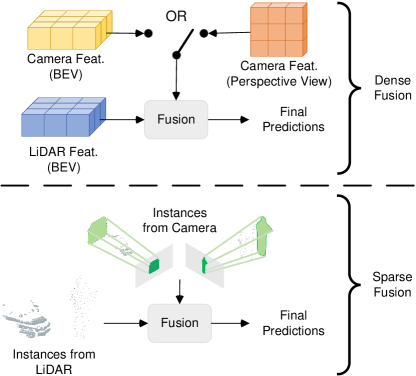
Figure 1: Comparison between dense fusion and sparse fusion. Dense fusion methods rely on LiDAR BEV feature maps for final prediction. In contrast, our sparse fusion framework unites two modalities at the instance level, requiring no dense feature map.

Autonomous driving systems heavily rely on 3D object detection. Currently, LiDARs and cameras are the two main sensors used for perception. LiDAR [60, 13, 15, 28] offers precise spatial positioning but struggles to recognize small and distant objects due to its sparsity nature. On the other hand, cameras [29, 19, 50] provide a wealth of semantic information but lack direct depth information. Combining this two sensors [30, 32, 1] leads to improved detection precision and makes the system more robust to different scenarios.

Currently, the predominant multi-modal methods [60, 13, 44] rely on dense LiDAR detectors. Dense LiDAR detectors imply the detectors construct dense Bird’s-Eye-View (BEV) feature maps for prediction. The size of these BEV feature maps increases quadratically with perception range, which leads to unaffordable costs in long-range detection. To address this issue, several voxel-based fully sparse detectors [14, 9, 33, 16] have emerged, largely extending the perception range of the LiDAR side. As a representative, FSD [14] demonstrates impressive efficiency and efficacy. However, incorporating multi-modal input needs a deliberate design for fully sparse structure. How to develop an effective and efficient multi-modal fully sparse detector is untapped. In this paper, we focus on extending the emerging fully sparse architecture into the domain of multi-modal detection.

A couple of options could be adopted to fuse image information into sparse detectors. The most straightforward one is point-wise painting [48, 49] with image features or semantic masks, which does not involve the dense BEV feature maps. However, the straightforward painting only utilizes semantic information, overlooking the instance-level information, which is important for the detection task. Fortunately, like other emerging detectors, FSD also follows the query-based paradigm, where the queries exactly correspond to 3D instances. This enlightens us to also construct the 2D instance queries to make the fusion unified as a query-based paradigm. In particular, we take the freebie from the well-studied 2D instance segmentation. The 2D instance masks are viewed as 2D queries, which are lifted to 3D space by gathering the corresponding point cloud in the frustum. In this way, these queries generated from images can be aligned with the queries from the LiDAR side, establishing a unified multi-modal input for further processing. As Fig. 1 shows, our design unites two structures from different modalities without incorporating any other feature-level view transformations, fulfilling our initial motivation of maintaining the fully sparse property.

In addition to the unified structure, our method also offers a good supplement for FSD, in which the 3D instance segmentation plays an essential but error-prone role. Without image information, the 3D instance segmentation itself is prone to miss non-discriminative foreground objects or mix crowded objects. Parallel to the 3D part, the queries generated from the 2D instance mask provide rich semantic information and strong instance-level hints, effectively alleviating such errors. This feature solely achieves a significant performance boost from the LiDAR-only version.

We summarize our contributions as follows:

• We propose a Fully Sparse Fusion (FSF) framework that first introduces the fully sparse architecture into multi-modal detection. FSF effectively unifies the two modalities within a sparse framework based on a query-based paradigm by integrating the well-studied 2D instance segmentation.

• The FSF achieves state-of-the-art performance on two large-scale datasets, nuScenes and Argoverse 2. Notably, FSF showcases superior efficiency in long-range detection (Argoverse 2) over other state-of-the-art multimodal 3D detectors.

2 Related Work

2.1 Camera-based 3D detection

In the early years of camera-based 3D detection, the focus is mainly on monocular 3D detection [2, 34, 63, 36, 25, 11]. However, monocular 3D detection ignores the relationships between cameras. To this end, more and more researchers are engaged in multi-view 3D detection. Multi-view 3D detection [24, 17] contains two main types of approaches: BEV-based and learnable-query-based. BEV-based methods [43, 29] lift 2D features to 3D [38, 19, 26] or using transformer-like structures [29, 57, 50] to construct BEV feature map for prediction. On the contrary, learnable-query-based methods [51, 31, 52] predict 3D bounding boxes from learnable queries.

2.2 LiDAR-based 3D detection

Although camera-based 3D detection methods achieve great results, their performance is still inferior to LiDAR-based 3D detection methods. LiDAR-based methods [22, 65] usually convert irregular LiDAR points into regular space for feature extraction. PointPillar [22], VoxelNet [65] and 3DFCN [23] employ dense convolution to extract features. However, utilizing dense convolution introduces heavy computational cost. To address this issue, SECOND [56] applies sparse convolution to 3D detection and inspires an increasing number of methods [60, 44, 8, 7] adopting sparse convolution for feature extraction. However, even with sparse convolution, most methods [60, 64] still require a dense feature map to alleviate the so-called “center feature missing” issue [14]. Researchers have been dedicated to developing fully sparse methods since point clouds are naturally sparse in 3D space. The pioneering works in this domain are PointNet-like methods [41, 42, 59, 39, 45]. Also, range view [15, 47] requires no BEV feature map, though their performance is inferior. Recently, a fully sparse 3D detection algorithm named FSD [14] has been proposed. FSD has demonstrated faster speed and higher accuracy than previous methods. Our work is based on FSD.

2.3 Multi-modal 3D detection

The multimodal 3D detection approaches can be classified into two types, namely dense and sparse, depending on whether it relies on the dense BEV feature map. As the representation of dense frameworks, BEVFusion [32, 30] fuses the BEV feature maps generated from camera and LiDAR modalities. Another line of dense fusion frameworks [1, 62, 21, 5] relies on the BEV feature map to generate proposals. The sparse approach, on the other hand, does not rely on dense feature maps. The most popular approaches are the point-level methods [48, 20, 55], which project LiDAR points onto the image plane to obtain image semantic cues. PointPainting [48] paints semantic scores, while PointAugmenting [49] paints features. Also, there are plenty of instance-level fusion [37, 27, 10] methods. MVP [61] uses instance information to produce virtual points to enrich point clouds. FrustumPointNet [40] and FrustumConvnet [53] utilize frustums to generate proposals. These methods work without relying on dense feature maps.

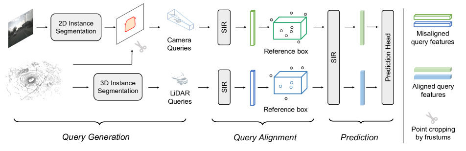
Figure 2: Overview of our framework. First, Bi-Modal Query Generation in §4.2 generates queries from two modalities. Then, these queries are aligned by the Query Alignment module in §4.3. Finally, the results are predicted by these aligned query features.

3 Preliminary: Fully Sparse 3D Detector

We first briefly introduce the emerging fully sparse 3D object detector FSD [14], which is adopted as our LiDAR-only baseline.

3D Instance Segmentation

Given LiDAR point clouds, FSD first performs 3D instance segmentation to produce 3D instances. Specifically, FSD extracts voxel features from the point cloud using a sparse voxel encoder in the beginning. Then the voxel features are mapped into their included points to build the point features. Using these point features, FSD classifies the points and only retains the foreground points. The retained foreground points predict their corresponding object centers, making the points belonging to the same object closer to each other. This process is called Voting [39]. After that, a Connected Components Labeling (CCL) algorithm is leveraged to obtain 3D instances by connecting the voted centers to form point clusters. The obtained point clusters are viewed as 3D instances.

Sparse Prediction

Given these instances, a point-based instance feature extractor, named Sparse Instance Recognition (SIR) module is utilized for feature extraction. The input of SIR is the feature of every point in the instance. Then a VFE-like [65] structure is used to produce high-quality instance features. Finally, 3D bounding boxes are produced by a simple MLP head.

The structure mentioned above does not involve any dense BEV feature maps. Thus it can be easily extended to long-range scenarios. However, how to equip the fully sparse architecture with rich image semantics is still under investigation. In the following section, we will describe our Fully Sparse Fusion (FSF) framework which first introduces the fully sparse architecture into multi-modal detection.

4 Methodology

4.1 Overall Architecture

The overall architecture of FSF is shown in Fig. 2. The framework could be roughly divided into two parts: the Bi-Modal Query Generation module in §4.2 and the Bi-Modal Query Refinement module in §4.3. The former generates queries specific to each modality. Afterwards, the latter aligns and refines the queries from different modalities to predict high-quality detection results.

4.2 Bi-modal Query Generation

LiDAR Queries

For the LiDAR modality, we adopt the 3D instance segmentation method in FSD to produce 3D instances. We refer these instances as LiDAR queries, and we define the position of a query as its centroid.

Camera Queries

3D instance segmentation is subjected to the sparsity of the point cloud and the lack of semantic information. The segmentation is prone to miss objects when the point cloud is too sparse. Moreover, in the scene where the instances are too crowded, it is easy to cluster multiple objects into one cluster as shown in Fig. 3. To tackle this problem, we utilize 2D instance segmentation to address the limitations of 3D instance segmentation. Specifically, we use the instance masks from well-studied 2D instance segmentation to generate initial frustums. We then crop the points within frustums to form point clusters. Note that frustums might overlap with each other, so we make copies of those points falling into the overlaps regions of each frustum. These point clusters can also be viewed as 3D instances, but they have totally different shapes from the ones from the LiDAR side. We will discuss the detailed solution in §4.3. For now, we name such coarse 3D instances generated from frustums as camera queries. We define the center of a camera query as the weighted average of all points in this instance. The weights are the classification scores from 3D instance segmentation.

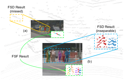
Figure 3: (a): 3D instance segmentation is prone to ignore distant objects. (b): It is hard for 3D segmentation to separate the overlapped objects in a crowded scene. On the contrary, it is easy to handle these cases via 2D instance segmentation.

So far, we obtain two sets of queries from LiDAR and camera, respectively. They are in a consistent form that is in fact the 3D instance, facilitating a unified query feature extraction and prediction pipeline. In addition, the two kinds of queries are complementary to each other due to the different nature of their sources.

4.3 Bi-modal Query Refinement

Query Alignment Although these two kinds of queries are in a consistent form, they might contain point clusters with totally different shapes. To unify these two kinds of queries, we must first align their shapes to simplify the pipeline and enable more effective feature learning. To this end, we propose to predict reference boxes from these queries. Then the reference boxes are used to correct the misaligned point cloud shape by further cropping points. Particularly, we apply SIR in FSD, a VFE-like module, on both of the two kinds of point clusters (i.e., queries) to extract the cluster features. Eventually, we use the extracted cluster features to predict the reference boxes.

Query Prediction So far, the queries generated from the two modalities are aligned in the form of reference 3D bounding boxes. These boxes are utilized to crop points and then extract the box features by another SIR module. The extracted box features are then used for the final classification and bounding box regression.

4.4 Query Label Assignment

FSD develops a simple yet effective assignment strategy, which regards queries falling into GT boxes as positive, and we name this strategy query-in-box assignment. However, this strategy could hardly work for camera queries for two reasons.

• The positions (i.e., cluster centroids) of camera queries are prone to have larger errors along the depth direction as Fig. 4 shows. The large error may be caused by overlapped foreground objects or background points in the frustum. After the query alignment, the reference boxes from camera queries have smaller variances but still are likely to be out of the GT boxes. In this circumstance, query-in-box assignment may cause a considerable amount of camera queries to be mistakenly assigned as negative.

• Due to the potential error of 2D instance segmentation and camera calibrations, a single frustum may contain multiple GTs, causing ambiguity in the assignment.

To address these two issues, we propose a 3D/2D two-round assignment.

Method	Modality	val		test
		mAP $\uparrow$	NDS $\uparrow$	mAP $\uparrow$	NDS $\uparrow$	mATE $\downarrow$	mASE $\downarrow$	mAOE $\downarrow$	mAVE$~{}\downarrow$	mAAE$~{}\downarrow$
DETR3D [51]	C	34.9	43.4	41.2	47.9	0.641	0.255	0.394	0.845	0.133
BEVDet4D [19]	C	42.1	54.5	45.1	56.9	0.511	0.241	0.386	0.301	0.121
BEVFormer [29]	C	41.6	51.7	48.1	56.9	0.582	0.256	0.375	0.378	0.126
SECOND [56]	L	52.6	63.0	52.8	63.3	-	-	-	-	-
CenterPoint [60]	L	59.6	66.8	60.3	67.3	0.262	0.239	0.361	0.288	0.136
FSD∗ [14]	L	62.5	68.7	-	-	-	-	-	-	-
VoxelNeXt [9]	L	63.5	68.7	64.5	70.0	0.268	0.238	0.377	0.219	0.127
TransFusion-L [1]	L	64.9	69.9	65.5	70.2	0.256	0.240	0.351	0.278	0.129
LargeKernel3D [8]	L	63.3	69.1	65.3	70.5	0.261	0.236	0.319	0.268	0.133
FUTR3D [6]	C+L	64.5	68.3	-	-	-	-	-	-	-
MVP [61]	C+L	67.1	70.8	66.4	70.5	0.263	0.238	0.321	0.313	0.134
PointAugmenting [49]	C+L	-	-	66.8	71.0	0.254	0.236	0.362	0.266	0.123
TransFusion [1]	C+L	67.5	71.3	68.9	71.6	0.259	0.243	0.359	0.288	0.127
BEVFusion [30]	C+L	67.9	71.0	69.2	71.8	-	-	-	-	-
BEVFusion [32]	C+L	68.5	71.4	70.2	72.9	0.261	0.239	0.329	0.260	0.134
DeepInteraction [58]	C+L	69.9	72.6	70.8	73.4	0.257	0.240	0.325	0.245	0.128
FSF (Ours)	C+L	70.4	72.7	70.6	74.0	0.246	0.234	0.318	0.211	0.123

Table 1: Comparison with state-of-the-art methods on the nuScenes dataset. We do not use test-time augmentation or model ensemble. ^∗: Reimplemented by us. We mark the official benchmark of nuScenes as Gray. C: camera modality. L: LiDAR modality.

3D Round

We first give higher priority to the assignment in 3D space. Particularly, for all queries, we first straightforwardly assign GTs to these queries by the query-in-box strategy in 3D space. This round not only makes our method consistent with the original LiDAR-only FSD, but also assigns accurate labels to the major part of camera queries.

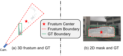
Figure 4: The motivation of 3D/2D two-round assignment. The center of a camera query is hard to fall into GT boxes as (a) shows. However, it is easy to assign this camera query to the corresponding GT on the 2D plane as (b) demonstrates.

2D Round

Complementary to the 3D round, we assign labels in 2D image space for another round. This round is designed for those unassigned camera queries. In practice, for each camera query, we have a 2D bounding box produced by 2D instance segmentation. We calculate the IoU between this 2D box and the projected 3D GTs. Then we follow the commonly-used “max IoU” strategy to assign labels. Specifically, for each ground-truth (GT) box, the “max IoU” assignment method compares this GT box with all the camera query boxes. If the IoU between a query box and this GT box is above a certain threshold, this camera query will be assigned to the GT. Eventually, after these two rounds, those samples still not associated with any GTs are assigned as negative.

To summarize, in our framework, we assign labels to queries in two rounds. The first one is to assign labels to the initially generated queries by query-in-box strategy. The second one is to assign labels to reference boxes via 2D IoU. For the Query Generation module and the Query Refinement module, we adopt the same two-round strategy for assignments.

4.5 Detection Head and Loss

Our framework comprises a total of three heads. These three heads are dedicated to generating LiDAR reference bounding boxes, camera reference bounding boxes, and final bounding boxes, respectively. The structures of these heads are the same. Each head is divided into two branches, namely regression branch and classification branch.

The regression branch takes each query’s feature as input, outputs $(\Delta x$, $\Delta y$, $\Delta z$, $\log{w}$, $\log{l}$, $\log{h}$, $\sin{r_{y}}$, $\cos{r_{y}})$. $(\Delta x,\Delta y,\Delta z)$ means the predicted offset from query’s center. $(w,l,h)$ means the dimension of the predicted box. $r_{y}$ is the heading angle in the yaw direction. We use $L1$ loss for regression branches and focal loss for classification branches, respectively.

Formally, we have regression loss $\mathcal{L}^{Li}_{reg}$, $\mathcal{L}^{Cam}_{reg}$, $\mathcal{L}^{Ref}_{reg}$ and classification loss $\mathcal{L}^{Li}_{cls}$, $\mathcal{L}^{Cam}_{cls}$, $\mathcal{L}^{Ref}_{cls}$ for LiDAR reference bounding boxes generation, camera reference bounding boxes generation and refined boxes generation, respectively.

In total, we have

$$\begin{split}\mathcal{L}_{total}=\mathcal{L}^{Li}_{seg}+\mathcal{L}^{Li}_{vote}+\mathcal{L}^{Li}_{cls}+\mathcal{L}^{Li}_{reg}\\ +\mathcal{L}^{Cam}_{cls}+\mathcal{L}^{Cam}_{reg}+\mathcal{L}^{Ref}_{cls}+\mathcal{L}^{Ref}_{reg},\end{split}$$ (1)

where $\mathcal{L}^{Li}_{seg}$ and $\mathcal{L}^{Li}_{vote}$ is the segmentation and voting loss of FSD. We omit the weight factors for each loss for brevity.

5 Experiments

5.1 Setup

	Methods	Average	Vehicle	Bus	Pedestrian	Box Truck	C-Barrel	Motorcyclist	MPC-Sign	Motorcycle	Bicycle	A-Bus	School Bus	Truck Cab	C-Cone	V-Trailer	Bollard	Sign	Large Vehicle	Stop Sign	Stroller	Bicyclist
mAP	CenterPoint‡ [60]	13.5	61.0	36.0	33.0	26.0	22.5	16.0	16.0	12.5	9.5	8.5	7.5	8.0	8.0	7.0	25.0	6.5	3.0	28.0	2.0	14
	CenterPoint∗ [60]	22.0	67.6	38.9	46.5	40.1	32.2	28.6	27.4	33.4	24.5	8.7	25.8	22.6	29.5	22.4	37.4	6.3	3.9	16.9	0.5	20.1
	FSD [14]	28.2	68.1	40.9	59.0	38.5	42.6	39.7	26.2	49.0	38.6	20.4	30.5	14.8	41.2	26.9	41.8	11.9	5.9	29.0	13.8	33.4
	VoxelNeXt [9]	30.5	72.0	39.7	63.2	39.7	64.5	46.0	34.8	44.9	40.7	21.0	27.0	18.4	44.5	22.2	53.7	15.6	7.3	40.1	11.1	34.9
	FSF (Ours)	33.2	70.8	44.1	60.8	40.2	50.9	48.9	28.3	60.9	47.6	22.7	36.1	26.7	51.7	28.1	41.1	12.2	6.8	27.7	25.0	41.6
CDS	CenterPoint∗ [60]	17.6	57.2	32.0	35.7	31.0	25.6	22.2	19.1	28.2	19.6	6.8	22.5	17.4	22.4	17.2	28.9	4.8	3.0	13.2	0.4	16.7
	FSD [14]	22.7	57.7	34.2	47.5	31.7	34.4	32.3	18.0	41.4	32.0	15.9	26.1	11.0	30.7	20.5	30.9	9.5	4.4	23.4	11.5	28.0
	VoxelNeXt [9]	23.0	57.7	30.3	45.5	31.6	50.5	33.8	25.1	34.3	30.5	15.5	22.2	13.6	32.5	15.1	38.4	11.8	5.2	30.0	8.9	25.7
	FSF (Ours)	25.5	59.6	35.6	48.5	32.1	40.1	35.9	19.1	48.9	37.2	17.2	29.5	19.6	37.3	21.0	29.9	9.2	4.9	21.8	18.5	32.0

Table 2: Comparison with state-of-the-art methods on Argoverse 2 validation split. C-Barrel: construction barrel. MPC-Sign: mobile pedestrian crossing sign. A-Bus: articulated bus. C-Cone: construction cone. V-Trailer: vehicular trailer. ‡: provided by authors of AV2 dataset. ^∗: reimplemented by FSD. Some categories are excluded from the table due to the limited number of instances they contain. However, the average results consider all categories, even those that are omitted.

Dataset: nuScenes

Our experiment is mainly conducted on the nuScenes dataset [3], which provides a total of 1000 scenes. Each scene is about 20 seconds long and contains collected data from 32-beam LiDAR along with 6 cameras. The effective detection range of nuScenes covers a $108m\times 108m$ area, and annotations are divided into 10 categories. In order to measure the performance in this dataset, the official metrics of nuScenes, Mean Average Precision (mAP) and nuScenes Detection Score (NDS) are utilized. The NDS is the weighted average of mAP, mATE (translation error), mASE (scale error), mAOE (orientation error), mAVE (velocity error), and mAAE (attribute error).

Dataset: Argoverse 2

To demonstrate our superiority in long-range detection, we proceed to conduct experiments on the Argoverse 2 dataset [54], abbreviated as AV2. The AV2 contains 150k annotated frames, 5$\times$ larger than nuScenes. AV2 employs two 32-beam LiDARs to form a 64-beam LiDAR, combined with 7 surrounding cameras. The valid detection distance of AV2 is 200m (covering $400m\times 400m$ area). In addition, AV2 contains 30 classes, exhibiting challenging long-tail distribution. As far as metrics are concerned, in addition to the Mean Average Precision (mAP), AV2 provides a Composite Detection Score (CDS) benchmark, which takes mAP, mATE, mASE, and mAOE into account.

Model

As for LiDAR, following FSD [14], we adopt a sparse-convolution-based U-Net [46] as the LiDAR backbone. The voxel size is set to $[0.2m,0.2m,0.2m]$. With respect to 2D instance segmentation, we use HybridTaskCascade (HTC) [4] pre-trained on nuImages. For the SIR module that utilized for instance feature extraction, we use the same setting as FSD [14].

Training Scheme

Next, we present the training strategy. Consistent with previous methods[1, 30], we first train the LiDAR-based detector. We pre-train FSD on nuScenes for 20 epochs with CopyPaste augmentation [56]. Next, initializing from FSD, we train our model for 6 epochs with CBGS [66]. The optimizer is AdamW [35]. We adopt the one-cycle learning rate policy, with a maximum learning rate of $10^{-4}$ and a weight decay of $10^{-2}$. The model is trained on eight NVIDIA RTX 3090 with batch size of 8.

5.2 Comparison with State-of-the-art Methods

nuScenes

As shown in Table 1, FSF surpasses all previous multi-modal 3D detection methods in the official NDS metric. It is noteworthy that state-of-the-art BEVFusion and DeepInteraction have inferior performance to FSF, even they [1, 58] utilize a stronger LiDAR-only detector (TransFusion-L).

Argoverse 2

AV2 has a much larger perception range than nuScenes, making it a suitable testbed to demonstrate our superiority in long-range fusion. The results in Table 2 show that FSF consistently outperforms previous LiDAR-based state-of-the-art methods by large margins. Notably, we observe an 8 to 10 mAP increase in categories with relatively small sizes, such as Traffic Cone, Motorcycle, and Bicycle. Although previous multi-modal methods (e.g., BEVFusion) achieve competitive results on nuScenes, the training cost of their dense BEV feature maps are not affordable on AV2 dataset. As a result, we omit their results on AV2.

5.3 Alternatives to FSF

As mentioned in §1, a couple of fusion methods can be adapted to fully sparse architecture. So, in this section, we reproduce these alternatives and conduct a comprehensive performance comparison between them and FSF.

Point Painting

The most straightforward approach is using PointPainting [48], where the 2D semantic scores are painted onto each point. The results in Table 3 show simple point painting could obtain considerable improvement but is largely inferior to FSF.

Feature Painting

Feature painting [49, 27, 10] alternatively paints image features to the point cloud. Features contain rich information than semantic masks. To reproduce a fair feature painting baseline with FSD, we utilize the multi-level image features from FPN of the HTC. The points are then decorated with these image features. Compared with score painting, feature painting has an improvement of 0.4 mAP.

Virtual Point

Similar to FSF, MVP [61] utilizes 2D instance segmentation to augment point clouds by adding additional virtual points on each instance. Then the augmented point clouds are sent into a LiDAR-based detector. We use the official code to generate virtual points. Table 3 demonstrates that adopting MVP achieves better performance than the painting method above, but is still worse than ours.

Discussion: why is FSF superior to the alternatives?

Although all three alternatives achieve considerable improvement on the LiDAR baseline, they are significantly worse than FSF. We owe the superior performance of FSF to two aspects:

• FSF not only enriches semantic information but also explicitly leverages instance information to correct the mistaken 3D instance segmentation, which might mix the crowded instances together as Fig. 3 shows.

• We align camera queries and LiDAR queries in a consistent form, so the prediction head could be shared between these two modalities, unleashing the potential of camera queries.

Method	Modality	mAP	NDS
FSD [14]	L	62.5	68.7
FSD + PointPainting [48]	L+C	66.9	70.9
FSD + Feature Painting [49]	L+C	67.3	71.2
FSD + MVP [61]	L+C	67.6	71.5
FSF	L+C	70.4	72.7

Table 3: Different fusion strategies for sparse detection architecture. PointPainting [48]: painting semantic scores. Feature Painting [49]: painting the image features. MVP [61]: employing virtual points to enhance point clouds.

5.4 Long Range Fusion

FSF achieves state-of-the-art performance on Argoverse 2 dataset, which has a very large perception range ($400m\times 400m$). Here we emphasize the superiority of FSF in long-range fusion by evaluating the inference latency and range-conditioned performance. The latency is tested on RTX 3090 with batch size 1. Our code is based on MMDetection3D [12] and the IO time is excluded.

Latency and Memory Footprint

Table 4 shows their computational and memory cost. FSF shows remarkable efficiency advantages over other state-of-the-art multi-modal methods since FSF does not incorporate any dense BEV feature maps. In contrast, previous art TransFusion [1] not only applies 2D convolutions on dense BEV feature maps, but also adopts global cross attention between queries and the whole BEV feature maps, leading to unacceptable latency.

Method	Modality	Latency (ms)	Memory (GB)
TransFusion-L [1]	L	320	14.5
CenterPoint [60]	L	232	8.1
FSD [14]	L	97	3.8
TransFusion [1]	C+L	384	17.3
Ours	C+L	141	6.9

Table 4: The inference latency and memory footprint of Argoverse 2 dataset, which covers $400m\times 400m$ area. We are even faster and use less memory than the BEV feature map based LiDAR-only methods.

In addition, as evidenced in Table 4, despite the need to process seven images, our approach remains faster and requires less memory footprint than LiDAR-only methods like CenterPoint [60].

Range-conditioned Performance

Table 5 demonstrates the performance conditioned on different perception ranges. The image is dense and of high resolution, making it helpful for detecting distant objects. As shown in Table 5, in the range spanning from 50m to 100m, we observe a remarkable improvement in mAP specifically for small objects, such as motorcyclists and bicyclists.

	Overall mAP	0m-50m				50m-100m
		Avg.	Motor.	Bicyc.	C.B.	Avg.	Motor.	Bicyc.	C.B.
FSD	28.1	41.6	57.3	57.4	66.1	10.9	8.8	17.0	13.8
FSF	33.2	45.3	57.9	65.1	73.7	17.2	36.4	31.1	25.2

Table 5: Performance of different ranges on Argoverse 2. FSF significantly improves the performance on faraway objects compared to the FSD [14]. Avg.: the average mAP of all classes. Motor.: Motorcyclist. Bicyc.: Bicyclist. C.B.: Construction Barrel.

5.5 Ablation Studies

Bi-modal Queries

Camera Queries	LiDAR Queries	Query Alignment	NDS	mAP	Car	Truck	Bus	Trailer	C.V.	Ped.	Motor.	Bicyc.	T.C.	Barrier
✓			68.8	63.1	80.5	54.3	72.1	34.6	29.0	85.4	72.3	68.8	78.0	64.0
	✓		68.7	62.5	83.9	56.4	73.4	41.4	27.4	84.3	69.5	55.6	72.4	60.7
✓	✓		71.5	68.6	85.2	60.2	75.0	41.5	32.9	87.4	77.2	72.0	80.1	74.1
✓	✓	✓	72.7	70.4	86.1	62.5	76.8	44.8	34.4	88.6	78.7	73.7	82.6	75.5

Table 6: Ablation study of the Query Generation and Query Alignment. C.V.: Construction Vehicle. Ped.: Pedestrian. Motor.: Motorcycle. Bicyc.: Bicycle. T.C: Traffic Cone. Gray Cell: By comparing LiDAR queries and camera queries, we highlight the results in which one performed better than the other.

Although the form of two kinds of queries is unified by query alignment, they still have different natures since they come from two different modalities. To reveal the pros and cons of the two kinds of queries, we remove each of them from FSF for ablation. There are several intriguing findings in Table 6.

• Camera queries are better in the categories with relatively small sizes. Especially, camera queries show significant advantages over LiDAR queries in Motorcycle, Bicycle, and Traffic cone. In contrast, LiDAR queries are better in the categories with large sizes, such as Car, Bus, and Trailer.

• Their differences make them complementary to each other. Combining two kinds of queries, the performance improves in all categories. It is noteworthy that the performance is also significantly improved in some classes where LiDAR queries and camera queries have similar performance, such as Bus and Pedestrian.

Query Alignment

To verify the effectiveness of our query alignment method, we design a model without query alignment, which we refer to as FSF-M (FSF-Misaligned). Specifically, to properly remove the query alignment while maintaining fairness, we still predict a reference box based on the initial camera queries but do not use the reference box to correct the shape of the point cluster. Thus, the only difference between FSF-M and FSF is that they have different cluster shapes in camera queries. Table 6 shows the comparison between FSF-M (the third row) and FSF , where query alignment gives us a 1.8 mAP boost. Without the alignment, the performance degrades in all categories consistently, which indicates the query alignment has an essential impact on the performance.

Two-round Assignment

Another essential difference between FSF and the LiDAR-only FSD is the proposed two-around assignment. To verify its effectiveness, we make comparisons between our strategy with two commonly used strategies: one-to-one assignment and query-in-box assignment, and the results are shown in Table 7. For the one-to-one assignment, we adopt the implementation from DETR3D [51] and add a self-attention module between queries following the convention. For the query-in-box assignment, we use the same hyperparameters with our 3D round. In the two experiments, all queries are treated equally. We reach two conclusions as follows.

• The model adopting one-to-one assignment fails to converge. This is because a considerable number of camera queries tightly overlap with LiDAR queries. It confuses the model learning if we only choose one as positive.

• The model using query-in-box assignment normally converges but shows an inferior performance to our default setting. We owe it to that the centroids of frustum have large variances along the depth direction, and are unlikely to accurately fall into 3D ground-truth boxes as Fig. 4 shows.

Assignment	mAP	NDS
One-to-one	Not converged	Not converged
Query-in-Box only	68.7	71.9
Two-round Assignment	70.4	72.7

Table 7: Ablation study of different assignment methods. This experiment reveals the importance of our two-round assignment.

Robustness against 2D Predictions

It would be a major concern whether FSF is robust to the 2D sides. To answer this question, we change the default HTC to a basic Mask RCNN whose 2D Mask AP on nuImages is only 38.4. As Table 8 shows, although the 2D performance has a significant drop after degrading the 2D part, the 3D performance of FSF only has 1 mAP drop. Besides, we also conduct an experiment that degrades 2D masks to 2D boxes during producing frustum. The result shows that downgrading the masks to boxes has minimal impact on 3D detection. It is reasonable since the camera queries go through further refinement in FSF , which mitigates the impact of inaccurate 2D results.

Method	2D in nuImage		Mask/Box	3D in nuScenes
	Mask∗	Box∗		mAP	NDS
Mask RCNN [18]	38.4	47.8	Mask	69.4	72.3
HTC [4]	46.4	57.3	Box	69.8	72.5
			Mask	70.4	72.7

Table 8: Ablation study of different 2D sides. Mask^∗: Mask mAP. Box^∗: Box mAP. The result reveals that our method is robust against the 2D predictions.

Image features	mAP	NDS	mATE	mASE	mAOE	mAVE	mAAE
$\times$	70.4	72.7	0.277	0.247	0.317	0.218	0.186
✓	70.7	72.9	0.274	0.247	0.307	0.223	0.187

Table 9: Ablation study of using the image feature. Utilizing image features does not result in a significant improvement. As a result, we make it an optional choice.

Does the image feature help more?

To answer this question, we conduct an experiment that adopts the same setting as §5.3, where each point is painted with the FPN’s multi-layered features. As shown in Table 9, using the image feature results in a marginal increase of 0.3 mAP in our approach. Therefore, we make it an optional choice to utilize the image feature or not, since it will introduce additional costs.

6 Conclusion

We propose a Fully Sparse Fusion (FSF) framework, a state-of-the-art 3D object detector that utilizes a Bi-Modal Query Generator for joint 2D and 3D instance segmentation. FSF then incorporates a Query Refinement module that effectively aligns and refines queries. Our framework achieves state-of-the-art performance on two large-scale datasets, nuScenes and Argoverse 2. Additionally, FSF significantly reduces latency and memory usage in long-range detection.

References

- [1] Xuyang Bai, Zeyu Hu, Xinge Zhu, Qingqiu Huang, Yilun Chen, Hongbo Fu, and Chiew-Lan Tai. TransFusion: Robust lidar-camera fusion for 3d object detection with transformers. In CVPR, 2022.
- [2] Garrick Brazil and Xiaoming Liu. M3D-RPN: Monocular 3d region proposal network for object detection. In ICCV, 2019.
- [3] Holger Caesar, Varun Bankiti, Alex H Lang, Sourabh Vora, Venice Erin Liong, Qiang Xu, Anush Krishnan, Yu Pan, Giancarlo Baldan, and Oscar Beijbom. nuScenes: A multimodal dataset for autonomous driving. In CVPR, 2020.
- [4] Kai Chen, Jiangmiao Pang, Jiaqi Wang, Yu Xiong, Xiaoxiao Li, Shuyang Sun, Wansen Feng, Ziwei Liu, Jianping Shi, Wanli Ouyang, et al. Hybrid task cascade for instance segmentation. In CVPR, 2019.
- [5] Xiaozhi Chen, Huimin Ma, Ji Wan, Bo Li, and Tian Xia. Multi-View 3D Object Detection Network for Autonomous Driving. In CVPR, 2017.
- [6] Xuanyao Chen, Tianyuan Zhang, Yue Wang, Yilun Wang, and Hang Zhao. FUTR3D: A unified sensor fusion framework for 3d detection. arXiv preprint arXiv:2203.10642, 2022.
- [7] Yukang Chen, Yanwei Li, Xiangyu Zhang, Jian Sun, and Jiaya Jia. Focal Sparse Convolutional Networks for 3D Object Detection. In CVPR, 2022.
- [8] Yukang Chen, Jianhui Liu, Xiaojuan Qi, Xiangyu Zhang, Jian Sun, and Jiaya Jia. Scaling up kernels in 3D CNNs. arXiv preprint arXiv:2206.10555, 2022.
- [9] Yukang Chen, Jianhui Liu, Xiangyu Zhang, Xiaojuan Qi, and Jiaya Jia. VoxelNeXt: Fully Sparse VoxelNet for 3D Object Detection and Tracking. In CVPR, 2023.
- [10] Zehui Chen, Zhenyu Li, Shiquan Zhang, Liangji Fang, Qinghong Jiang, Feng Zhao, Bolei Zhou, and Hang Zhao. Autoalign: Pixel-instance feature aggregation for multi-modal 3d object detection. ECCV, 2022.
- [11] Zhiyu Chong, Xinzhu Ma, Hong Zhang, Yuxin Yue, Haojie Li, Zhihui Wang, and Wanli Ouyang. MonoDistill: Learning spatial features for monocular 3D object detection. 2022.
- [12] MMDetection3D Contributors. MMDetection3D: OpenMMLab Next-generation Platform for General 3D Object Detection. https://github.com/open-mmlab/mmdetection3d, 2020.
- [13] Lue Fan, Ziqi Pang, Tianyuan Zhang, Yu-Xiong Wang, Hang Zhao, Feng Wang, Naiyan Wang, and Zhaoxiang Zhang. Embracing Single Stride 3D Object Detector with Sparse Transformer. In CVPR, 2022.
- [14] Lue Fan, Feng Wang, Naiyan Wang, and Zhaoxiang Zhang. Fully Sparse 3D Object Detection. In NeurIPS, 2022.
- [15] Lue Fan, Xuan Xiong, Feng Wang, Naiyan Wang, and ZhaoXiang Zhang. RangeDet: In Defense of Range View for LiDAR-Based 3D Object Detection. In ICCV, 2021.
- [16] Lue Fan, Yuxue Yang, Feng Wang, Naiyan Wang, and Zhaoxiang Zhang. Super sparse 3d object detection. arXiv preprint arXiv:2301.02562, 2023.
- [17] Xiaoyang Guo, Shaoshuai Shi, Xiaogang Wang, and Hongsheng Li. Liga-stereo: Learning Lidar Geometry Aware Representations for Stereo-based 3D Detector. In ICCV, 2021.
- [18] Kaiming He, Georgia Gkioxari, Piotr Dollár, and Ross Girshick. Mask R-CNN. In ICCV, 2017.
- [19] Junjie Huang and Guan Huang. BEVDet4D: Exploit temporal cues in multi-camera 3d object detection. arXiv preprint arXiv:2203.17054, 2022.
- [20] Tengteng Huang, Zhe Liu, Xiwu Chen, and Xiang Bai. EPNet: Enhancing point features with image semantics for 3D object detection. In ECCV, 2020.
- [21] Jason Ku, Melissa Mozifian, Jungwook Lee, Ali Harakeh, and Steven L Waslander. Joint 3D Proposal Generation and Object Detection from View Aggregation. In IROS, 2018.
- [22] Alex H Lang, Sourabh Vora, Holger Caesar, Lubing Zhou, Jiong Yang, and Oscar Beijbom. PointPillars: Fast Encoders for Object Detection from Point Clouds. In CVPR, 2019.
- [23] Bo Li. 3D Fully Convolutional Network for Vehicle Detection in Point Cloud. In IROS, 2017.
- [24] Peiliang Li, Xiaozhi Chen, and Shaojie Shen. Stereo R-CNN based 3d Object Detection for Autonomous Driving. In CVPR, 2019.
- [25] Yingyan Li, Yuntao Chen, Jiawei He, and Zhaoxiang Zhang. Densely Constrained Depth Estimator for Monocular 3D Object Detection. In ECCV, 2022.
- [26] Yinhao Li, Zheng Ge, Guanyi Yu, Jinrong Yang, Zengran Wang, Yukang Shi, Jianjian Sun, and Zeming Li. BevDepth: Acquisition of reliable depth for multi-view 3d object detection. In AAAI, 2023.
- [27] Yingwei Li, Adams Wei Yu, Tianjian Meng, Ben Caine, Jiquan Ngiam, Daiyi Peng, Junyang Shen, Bo Wu, Yifeng Lu, Denny Zhou, et al. DeepFusion: Lidar-Camera Deep Fusion for Multi-Modal 3D Object Detection. In CVPR, 2022.
- [28] Zhichao Li, Feng Wang, and Naiyan Wang. LiDAR R-CNN: An Efficient and Universal 3D Object Detector. In CVPR, 2021.
- [29] Zhiqi Li, Wenhai Wang, Hongyang Li, Enze Xie, Chonghao Sima, Tong Lu, Yu Qiao, and Jifeng Dai. BevFormer: Learning bird’s-eye-view representation from multi-camera images via spatiotemporal transformers. In ECCV, 2022.
- [30] Tingting Liang, Hongwei Xie, Kaicheng Yu, Zhongyu Xia, Zhiwei Lin, Yongtao Wang, Tao Tang, Bing Wang, and Zhi Tang. BEVFusion: A simple and robust lidar-camera fusion framework. In NeurIPS, 2022.
- [31] Yingfei Liu, Tiancai Wang, Xiangyu Zhang, and Jian Sun. PETR: Position embedding transformation for multi-view 3d object detection. In ECCV, 2022.
- [32] Zhijian Liu, Haotian Tang, Alexander Amini, Xinyu Yang, Huizi Mao, Daniela Rus, and Song Han. BEVFusion: Multi-Task Multi-Sensor Fusion with Unified Bird’s-Eye View Representation. In ICRA, 2023.
- [33] Zhijian Liu, Xinyu Yang, Haotian Tang, Shang Yang, and Song Han. FlatFormer: Flattened Window Attention for Efficient Point Cloud Transformer. In CVPR, 2023.
- [34] Zongdai Liu, Dingfu Zhou, Feixiang Lu, Jin Fang, and Liangjun Zhang. AutoShape: Real-time shape-aware monocular 3d object detection. In ICCV, 2021.
- [35] Ilya Loshchilov and Frank Hutter. Decoupled Weight Decay Regularization. arXiv preprint arXiv:1711.05101, 2017.
- [36] Yan Lu, Xinzhu Ma, Lei Yang, Tianzhu Zhang, Yating Liu, Qi Chu, Junjie Yan, and Wanli Ouyang. Geometry uncertainty projection network for monocular 3D object detection. In ICCV, 2021.
- [37] Su Pang, Daniel Morris, and Hayder Radha. CLOCs: Camera-LiDAR object candidates fusion for 3D object detection. In IROS, 2020.
- [38] Jonah Philion and Sanja Fidler. Lift, Splat, Shoot: Encoding images from arbitrary camera rigs by implicitly unprojecting to 3D. In ECCV, 2020.
- [39] Charles R Qi, Or Litany, Kaiming He, and Leonidas J Guibas. Deep Hough Voting for 3D Object Detection in Point Clouds. In ICCV, 2019.
- [40] Charles R Qi, Wei Liu, Chenxia Wu, Hao Su, and Leonidas J Guibas. Frustum PointNets for 3D Object Detection from RGB-D Data. In CVPR, 2018.
- [41] Charles R Qi, Hao Su, Kaichun Mo, and Leonidas J Guibas. PointNet: Deep Learning on Point Sets for 3D Classification and Segmentation. In CVPR, 2017.
- [42] Charles Ruizhongtai Qi, Li Yi, Hao Su, and Leonidas J Guibas. PointNet++: Deep Hierarchical Feature Learning on Point Sets in a Metric Space. In NeurIPS, 2017.
- [43] Cody Reading, Ali Harakeh, Julia Chae, and Steven L Waslander. Categorical depth distribution network for monocular 3D object detection. In CVPR, 2021.
- [44] Shaoshuai Shi, Chaoxu Guo, Li Jiang, Zhe Wang, Jianping Shi, Xiaogang Wang, and Hongsheng Li. PV-RCNN: Point-Voxel Feature Set Abstraction for 3D Object Detection. In CVPR, 2020.
- [45] Shaoshuai Shi, Xiaogang Wang, and Hongsheng Li. PointRCNN: 3D Object Proposal Generation and Detection from Point Cloud. In CVPR, 2019.
- [46] Shaoshuai Shi, Zhe Wang, Jianping Shi, Xiaogang Wang, and Hongsheng Li. From Points to Parts: 3D Object Detection from Point Cloud with Part-aware and Part-aggregation Network. IEEE Transactions on Pattern Analysis and Machine Intelligence, 2020.
- [47] Zhi Tian, Xiangxiang Chu, Xiaoming Wang, Xiaolin Wei, and Chunhua Shen. Fully convolutional one-stage 3D object detection on LiDAR range images. In NeurIPS, 2022.
- [48] Sourabh Vora, Alex H Lang, Bassam Helou, and Oscar Beijbom. PointPainting: Sequential Fusion for 3D Object Detection. In CVPR, 2020.
- [49] Chunwei Wang, Chao Ma, Ming Zhu, and Xiaokang Yang. Pointaugmenting: Cross-modal augmentation for 3d object detection. In CVPR, 2021.
- [50] Yuqi Wang, Yuntao Chen, and Zhaoxiang Zhang. FrustumFormer: Adaptive Instance-aware Resampling for Multi-view 3D Detection. 2023.
- [51] Yue Wang, Vitor Campagnolo Guizilini, Tianyuan Zhang, Yilun Wang, Hang Zhao, and Justin Solomon. DETR3D: 3D object detection from multi-view images via 3d-to-2d queries. In CoRL, 2022.
- [52] Zitian Wang, Zehao Huang, Jiahui Fu, Naiyan Wang, and Si Liu. Object as Query: Equipping Any 2D Object Detector with 3D Detection Ability. arXiv preprint arXiv:2301.02364, 2023.
- [53] Zhixin Wang and Kui Jia. Frustum ConvNet: Sliding frustums to aggregate local point-wise features for amodal 3d object detection. In IROS, 2019.
- [54] Benjamin Wilson, William Qi, Tanmay Agarwal, John Lambert, Jagjeet Singh, Siddhesh Khandelwal, Bowen Pan, Ratnesh Kumar, Andrew Hartnett, Jhony Kaesemodel Pontes, Deva Ramanan, Peter Carr, and James Hays. Argoverse 2: Next Generation Datasets for Self-Driving Perception and Forecasting. In NeurIPS Datasets and Benchmarks 2021, 2021.
- [55] Shaoqing Xu, Dingfu Zhou, Jin Fang, Junbo Yin, Zhou Bin, and Liangjun Zhang. FusionPainting: Multimodal fusion with adaptive attention for 3D object detection. In ITSC, 2021.
- [56] Yan Yan, Yuxing Mao, and Bo Li. SECOND: Sparsely Embedded Convolutional Detection. Sensors, 18(10), 2018.
- [57] Chenyu Yang, Yuntao Chen, Hao Tian, Chenxin Tao, Xizhou Zhu, Zhaoxiang Zhang, Gao Huang, Hongyang Li, Yu Qiao, Lewei Lu, et al. BEVFormer v2: Adapting Modern Image Backbones to Bird’s-Eye-View Recognition via Perspective Supervision. 2023.
- [58] Zeyu Yang, Jiaqi Chen, Zhenwei Miao, Wei Li, Xiatian Zhu, and Li Zhang. DeepInteraction: 3D object detection via modality interaction. In NeurIPS, 2022.
- [59] Zetong Yang, Yanan Sun, Shu Liu, and Jiaya Jia. 3DSSD: Point-based 3D Single Stage Object Detector. In CVPR, 2020.
- [60] Tianwei Yin, Xingyi Zhou, and Philipp Krähenbühl. Center-based 3D Object Detection and Tracking. In CVPR, 2021.
- [61] Tianwei Yin, Xingyi Zhou, and Philipp Krähenbühl. Multimodal virtual point 3d detection. In NeurIPS, 2021.
- [62] Jin Hyeok Yoo, Yecheol Kim, Jisong Kim, and Jun Won Choi. 3D-CVF: Generating joint camera and lidar features using cross-view spatial feature fusion for 3d object detection. In ECCV, 2020.
- [63] Yunpeng Zhang, Jiwen Lu, and Jie Zhou. Objects are different: Flexible monocular 3d object detection. In CVPR, 2021.
- [64] Hui Zhou, Xinge Zhu, Xiao Song, Yuexin Ma, Zhe Wang, Hongsheng Li, and Dahua Lin. Cylinder3D: An Effective 3D Framework for Driving-scene LiDAR Semantic Segmentation. In CVPR, 2021.
- [65] Yin Zhou and Oncel Tuzel. VoxelNet: End-to-End Learning for Point Cloud Based 3D Object Detection. In CVPR, 2018.
- [66] Benjin Zhu, Zhengkai Jiang, Xiangxin Zhou, Zeming Li, and Gang Yu. Class-balanced grouping and sampling for point cloud 3d object detection. arXiv preprint arXiv:1908.09492, 2019.