Explicit Correspondence Matching for Generalizable Neural Radiance Fields

Abstract

We present a new generalizable NeRF method that is able to directly generalize to new unseen scenarios and perform novel view synthesis with as few as two source views. The key to our approach lies in the explicitly modeled correspondence matching information, so as to provide the geometry prior to the prediction of NeRF color and density for volume rendering. The explicit correspondence matching is quantified with the cosine similarity between image features sampled at the 2D projections of a 3D point on different views, which is able to provide reliable cues about the surface geometry. Unlike previous methods where image features are extracted independently for each view, we consider modeling the cross-view interactions via Transformer cross-attention, which greatly improves the feature matching quality. Our method achieves state-of-the-art results on different evaluation settings, with the experiments showing a strong correlation between our learned cosine feature similarity and volume density, demonstrating the effectiveness and superiority of our proposed method. Code is at https://github.com/donydchen/matchnerf.

1 Introduction

In the past few years, we have seen rapid advances in photorealistic novel view synthesis with Neural Radiance Fields (NeRF) [22]. However, vanilla NeRF [22] and its variants [1, 2, 20, 41] are mainly designed for per-scene optimization scenarios, where the lengthy optimization time and the need for vast amounts of views for each scene limit their practical usages in real-world applications.

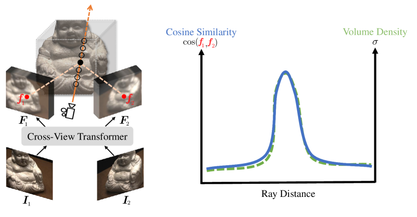
Figure 1: Correlation between cosine feature similarity and volume density. We first extract image features via a Transformer by considering cross-view interactions. Then, we explicitly fetch the correspondence feature matching information by computing the cosine similarity between sampled Transformer features, which shows strong correlation with volume density and thus provides valuable geometric cues for density prediction.

We are interested in a specific form of novel view synthesis, i.e., generalizable NeRF, which aims at learning to model the generic scene structure by conditioning the NeRF inputs on additional information derived from images [42, 8, 6]. This form has a wide range of applications, because it can generalize to new unseen scenarios, and can perform reasonably well with just a few (e.g., 3) camera views, while it does not require any retraining.

The existing generalizable NeRF approaches [49, 42, 38, 8, 6, 14, 16] generally adopt the pipeline of an image feature encoder that embeds multi-view images into a latent geometry prior $\bm{z}$, and a NeRF decoder that conditions on $\bm{z}$ to predict the 3D radiance field and volume-renders it to generate the target-view image. The key difference of these methods mainly lies in how the additional geometry prior is being encoded. Pioneer generalizable NeRF approaches [49, 42, 38] directly use and/or aggregate 2D convolutional image features independently extracted from each input source view, which struggle in new unseen scenarios, because their convolutional features are not explicitly geometry-aware. To address this issue, recent works [8, 6, 14, 16, 46] incorporate the geometry-aware multi-view consistency to encode the geometry prior. Among them, MVSNeRF [6] is the most representative one, which constructs a plane-sweep 3D cost volume followed by 3D Convolutional Neural Network (CNN) to generate the geometry prior $\bm{z}$, leveraging the success in multi-view stereo architectures [47, 10]. However, the construction of cost volume in MVSNeRF relies on a predefined reference view, resulting in poor performance (see Fig. 5) if the synthesized view does not have sufficient overlap with the reference view. MVSNeRF also suffers from noisy backgrounds (see Fig. 3) due to the cost volume.

The limitations of cost volume-based methods motivate us to turn back to the 2D image features for a simple and effective generalizable NeRF alternative. Our key idea is to explicitly match 2D image features across different views and use the correspondence matching statistics as the geometry prior $\bm{z}$. This is meaningful because the feature matching (i.e., the cosine similarity) of 2D projections of a 3D point reflects the multi-view consistency, which encodes the scene geometry and correlates well with the volume density (see Fig. 1). One key observation we have is that the 2D image features need to be aligned across different views, which can be effectively done via Transformer cross-attention over pairs of views. Another latest work GPNR [32] also uses 2D Transformer blocks to implicitly obtain correspondence matching by aggregating features along the epipolar line and across different views, and then predicts pixel colors using the fused features. In contrast, our method explicitly computes feature correspondence matching as cosine similarity for the NeRF conditional inputs. By providing NeRF with explicit geometry cues, our model manages to generalize to new scenes in a more effective and efficient manner (see Tab. 1b and Tab. 4).

Specifically, we explicitly compute multi-view correspondence matching from features extracted via self- and cross-attention of a Transformer, responsible for modeling the self- and cross-view interactions. One off-the-shelf tool is GMFlow [44], which is originally designed to estimate the optical flow, finding dense correspondence between two images. We extend its encoder to handle arbitrary views for multi-view inputs by processing the features in a pair-wise manner. Each pair of features are fed into the Transformer together to extract stronger and aligned features. In particular, for each 3D point, we project it into different views based on the given camera parameters, and bilinearly sample the Transformer features. We then compute the cosine similarity of sampled features in a pair-wise manner. To improve the expressiveness of cosine similarity, we compute it in a group-wise manner along the channel dimension, similar to [11, 45]. Finally, the averaged group-wise cosine similarity is fed into the NeRF decoder along with the original NeRF coordinate input to predict color and density. We demonstrate the superiority of our proposed method by thorough ablations and extensive experiments under several different evaluation settings.

Our major contributions can be summarized as follows:

• We propose to explicitly match 2D image features across different views and use the correspondence feature matching statistics as the geometry prior instead of constructing 3D cost volumes for generalizable NeRF.

• We propose to implement the explicit correspondence matching as the simple group-wise cosine similarity between image features, which are aligned via Transformer cross-attention for cross-view interactions.

• Our method is view-agnostic, unlike popular cost volume-based approaches that are typically sensitive to reference view selection. We achieve state-of-the-art results on standard benchmarks including DTU [13], Real Forward-Facing (RFF) [22] and Blender [22].

2 Related Work

Novel view synthesis via NeRF. With the powerful ability in modeling a continuous 3D field and volume rendering techniques [15], Neural Radiance Field (NeRF) [22] paved a new way for solving novel view synthesis by embedding the scene information as a neural implicit representation with the input of coordinates and view direction. However, vanilla NeRF requires many calibrated images and a lengthy time for optimization on each specific scene. Recent attempts have been made to make NeRF applicable, including reducing the training time with better data structure [33, 48, 23, 5, 36], reducing the number of images using additional regularization terms [12, 24, 39, 9, 50, 7].

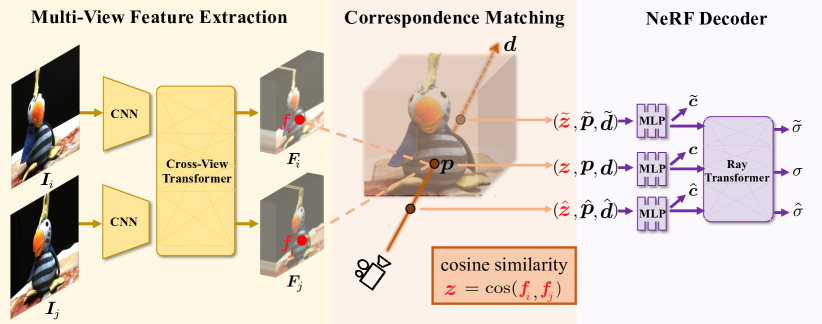
Figure 2: MatchNeRF overview. Given $N$ input images, we extract the Transformer features and compute the cosine similarity in a pair-wise manner, and finally merge all pair-wise cosine similarities with element-wise average. i@) For image pair ${\bm{I}}_{i}$ and ${\bm{I}}_{j}$, we first extract downsampled convolutional features with a weight-sharing CNN. The convolutional features are then fed into a Transformer to model cross-view interactions with cross-attention (Sec. 3.1). ii@) To predict the color and volume density of a point on a ray for volume rendering, we project the 3D point into the 2D Transformer features ${\bm{F}}_{i}$ and ${\bm{F}}_{j}$ with the camera parameters and bilinearly sample the feature vectors ${\bm{f}}_{i}$ and ${\bm{f}}_{j}$ at the projected locations. We then compute the cosine similarity ${\bm{z}}=\cos({\bm{f}}_{i},{\bm{f}}_{j})$ between sampled features to encode the correspondence matching information (Sec. 3.2). iii@) ${\bm{z}}$ is next used with the 3D position $\bm{p}$ and 2D view direction $\bm{d}$ for color $\bm{c}$ and density $\sigma$ prediction. An additional ray Transformer is used to model cross-point interactions along a ray (Sec. 3.3).

Generalizable NeRF from a learned prior. Pioneer works [49, 42, 8, 38] resort to intuitively condition NeRF on 2D features independently extracted from each input view, which however results in poor visual quality for unseen scenes due to the lack of explicit geometry-aware encoding. Following approaches [6, 14, 16] demonstrate that introducing a geometric prior could improve the generalization. In particular, MVSNeRF [6] builds a 3D cost volume with 3D CNN for post-regularization. However, such a cost volume-based geometry prior is sensitive to the selection of the reference view. GeoNeRF [14] improves MVSNeRF by fusing several cascaded cost volumes with attention modules, which complicates the full architecture, yet might still suffer from the inherent limitation of the cost volume representation. In contrast, we introduce a matching-based strategy to incorporate geometry prior without requiring 3D cost volume nor the subsequent 3D CNN, and it is view-agnostic.

Transformer in NeRF. Recently, there are a few methods that attempt to incorporate the Transformer [40] architecture to the NeRF model. NerFormer [29] proposes to use a Transformer to aggregate the features between different views on a ray and learn the radiance fields from the aggregated feature. IBRNet [42] proposes a ray Transformer to aggregate the information on a ray in the NeRF decoder. More recently, GNT [34] proposes to directly regress the color for view synthesis without NeRF’s volume rendering. GPNR [32] aggregates features with several stacked “patch-based” Transformers to improve generalization by avoiding potential harmful effects caused by CNN. Unlike all the above methods, ours mainly uses Transformer in the encoder to enhance the features with cross-view interaction, so that it can better serve the following correspondence matching process, aiming to provide a better geometry prior.

3 Methodology

Our goal is to learn a generalizable NeRF that synthesizes novel views for unseen scenes with few input views. This task is conceptually built on vanilla NeRF [22], except that here the model is trained for a series of scenes, rather than optimizing the model for each scene. Once trained, the model can produce high-quality novel views for conditional inputs, without the need for retraining. In particular, given $N$ views $\mathcal{I}=\{{\bm{I}}_{i}\}^{N}_{i=1}$ of a scene and corresponding camera parameters $\mathcal{M}=\{{\bm{M}}_{i}\}^{N}_{i=1}$, most generalizable NeRF approaches [8, 14, 42, 6] can be formulated as finding the functions of view fusion $f_{\theta}$ and view rendering $g_{\phi}$,

$$f_{\theta}:(\mathcal{I},\mathcal{M})\to{\bm{z}},\quad g_{\phi}:({\bm{p}},{\bm{d}},{\bm{z}})\to({\bm{c}},\sigma),$$ (1)

where $\bm{p}$ and $\bm{d}$ are the 3D point position and the 2D ray direction of a target viewpoint, $\bm{c}$ and $\sigma$ are the predicted color and density, which are used to render the target novel view via volume rendering (Sec. 3.3) as in the vanilla NeRF model. The key difference with vanilla NeRF is that additional information $\bm{z}$ is injected to provide the geometry prior, which is usually derived from images ($\mathcal{I}$ and $\mathcal{M}$). The functions $f_{\theta}$ and $g_{\phi}$ are typically parameterized with deep neural networks, where $\theta$ and $\phi$ denote the learnable parameters of the networks.

Previous generalizable NeRF approaches [8, 14, 42, 6] in general vary in how the additional information $\bm{z}$ is encoded with different networks $f_{\theta}$. In this research, we propose to explicitly match 2D image features across different views and use the correspondence matching statistics as the geometry prior $\bm{z}$, for which we name our method as MatchNeRF. Fig. 2 gives an overview of our proposed MatchNeRF framework. It consists of a Transformer encoder $f_{\theta}$ to extract cross-view aligned features, an explicit cosine similarity computation operation to obtain the correspondence matching information for the geometry prior $\bm{z}$, and a NeRF decoder $g_{\phi}$ with a ray Transformer to predict the color and density for volume rendering.

3.1 Multi-View Feature Extraction

For $N$ input views $\{{\bm{I}}_{i}\}^{N}_{i=1}$, we first extract $8\times$ downsampled convolutional features $\{{\bm{F}}^{\mathrm{c}}_{i}\}^{N}_{i=1}$ for each view independently, using a weight-sharing CNN. Unlike previous generalizable NeRF approaches [49, 42, 6] that are solely dependent on the per-view convolutional features, we further improve the feature quality by modeling the cross-view interactions between different views. This is achieved through a Transformer with cross-attention, for which we build upon the GMFlow’s [44] Transformer architecture. Compared with GMFlow, ours can handle arbitrary views for novel view synthesis in a pair-wise manner, instead of working only for fixed two views in the optical flow setting.

More specifically, we consider all the possible 2-view combinations of $N$ views and obtain a total of $N(N-1)/2$ view pairs. Each pair of convolutional features is fed into a weight-sharing Transformer jointly to consider their cross-view interactions, which can be described as

$$\mathcal{T}:({\bm{F}}^{\mathrm{c}}_{i},{\bm{F}}^{\mathrm{c}}_{j})\to({\bm{F}}_{i},{\bm{F}}_{j}),\quad\forall i,j\in\{1,2,\cdots,N\},i<j,$$ (2)

where $\mathcal{T}$ denotes the Transformer, which is composed of six stacked Transformer blocks, where each Transformer block contains self-, cross-attention and feed-forward networks following GMFlow [44]. We also add the fixed sine and cosine positional encodings to the convolutional features ${\bm{F}}^{\mathrm{c}}_{i}$ and ${\bm{F}}^{\mathrm{c}}_{j}$ before computing the attentions to inject the positional information [4]. We compute the attentions in a shifted local window [17] manner for better efficiency.

Thus far the features extracted from the Transformer are at $1/8$ of the original image resolution, which is lower than the $1/4$ resolution used in MVSNeRF [6], and thus might be unfavorable for our method. To remedy this, we align our highest feature resolution with MVSNeRF by using an additional convolutional upsampler to do $2\times$ upsampling of our $1/8$ features. In this way, we obtain both $1/8$ and $1/4$ resolution features. This simple upsampler leads to notable improvements as we show in our experiments Tab. 1d. We denote all the $1/4$ resolution feature pairs after upsampling as $(\hat{\bm{F}}_{i},\hat{\bm{F}}_{j}),i,j\in\{1,2,\cdots,N\},i<j$.

3.2 Correspondence Matching

To further provide geometric cues for volume density prediction, we compute the cosine similarity between sampled Transformer features as the correspondence matching information. Specifically, for a given 3D point position $\bm{p}$, we first project it onto the 2D Transformer features ${\bm{F}}_{i}$ and ${\bm{F}}_{j}$ ($i,j\in\{1,2,\cdots,N\},i<j$) of views $i,j$ using the camera parameters ${\bm{M}}_{i}$ and ${\bm{M}}_{j}$, and then bilinearly sample the corresponding feature vectors ${\bm{f}}_{i}$ and ${\bm{f}}_{j}$ at the specific 2D positions. We compute the cosine similarity between sampled Transformer features ${\bm{f}}_{i}$ and ${\bm{f}}_{j}$ to measure the multi-view consistency so as to provide the NeRF decoder information about whether the 3D point $\bm{p}$ is on the surface or not. However, the basic cosine similarity merges two high-dimensional feature vectors to a single scalar, which might lose too much information (see Tab. 1b). To further improve its expressiveness, we calculate the cosine similarity in a group-wise manner along the channel dimension [11]. Specifically, the feature vectors ${\bm{f}}_{i}$ and ${\bm{f}}_{j}$ are first equally partitioned into $G$ groups, and we then compute the cosine similarity between features in each group:

$${s}^{(g)}=\frac{{\bm{f}}_{i}^{(g)}\cdot{\bm{f}}_{j}^{(g)}}{\left\|{\bm{f}}_{i}^{(g)}\right\|_{2}\cdot\left\|{\bm{f}}_{j}^{(g)}\right\|_{2}},\quad g=1,2,\cdots,G,$$ (3)

where $(g)$ denotes the $g$-th group. All the cosine similarities are collected as a vector $\bm{s}=({s}^{(1)},{s}^{(2)},\cdots,{s}^{({G})})\in\mathbb{R}^{{G}}$.

Recall that the Transformer features are extracted at both $1/8$ and $1/4$ resolutions. Similarly we compute group-wise cosine similarity between the $1/4$ resolution features $\hat{\bm{F}}_{i}$ and $\hat{\bm{F}}_{j}$, $i,j\in\{1,2,\cdots,N\},i<j$, and accordingly we obtain another similarity $\hat{\bm{s}}=({\hat{s}}^{(1)},{\hat{s}}^{(2)},\cdots,{\hat{s}}^{(\hat{G})})\in\mathbb{R}^{\hat{G}}$ for $\hat{G}$ groups. We then concatenate ${\bm{s}}$ and $\hat{\bm{s}}$ and obtain the cosine similarity ${\bm{s}}_{i,j}\in\mathbb{R}^{G+\hat{G}}$ for view pair $(i,j)$.

This process is repeated for all the view pairs $(i,j),i,j\in\{1,2,\cdots,N\},i<j$ for a total of $N$ views, and the final cosine similarity is obtained by taking an element-wise average over all $N(N-1)/2$ pairs:

$$\bm{z}=\frac{\sum_{ij}{\bm{s}}_{ij}}{N(N-1)/2}\in\mathbb{R}^{G+\hat{G}},$$ (4)

where $\bm{z}$ is the geometry prior of our method, capturing the explicit correspondence matching information.

3.3 NeRF Decoder

The cosine similarity $\bm{z}$ in Eq. (4) constructed from the encoder $f_{\theta}$ is fed into the NeRF decoder $g_{\phi}$ for predicting NeRF color and density, as formulated in Eq. (1).

Rendering network. We follow prior works [49, 6] to construct a MLP-based rendering network. Similarly, we also include the texture priors by concatenating the color information sampled on all input views with the given position. But unlike the typical MLP decoder that processes all points on a ray independently, we further explore introducing cross-point interactions by fusing the rendered information along a ray via a Transformer. We adopt IBRNet’s [42] ray Transformer in our implementation for convenience.

Volume rendering. With the emitted color $\bm{c}$ and volume density $\sigma$ predicted by the rendering network, novel views can be synthesized via volume rendering, which is implemented with differential ray marching as in NeRF [22]. Specifically, to estimate the color ${\bm{C}}$ of a pixel, radiance needs to be accumulated across all sampled shading points on the corresponding ray that passes through the pixel,

$${\bm{C}}=\sum_{i=1}^{K}T_{i}(1-\textrm{exp}(-\sigma_{i}\delta_{i}))\bm{c}_{i},\quad T_{i}=\textrm{exp}(-\sum_{j}^{i-1}\sigma_{j}\delta_{j}),$$ (5)

where $\bm{c}_{i},\sigma_{i}$ refer to the color and density of the $i$-th sampled 3D point on the ray. $T_{i}$ is the volume transmittance and $\delta_{i}$ denotes the distances between adjacent points. $K$ is the total number of sampled 3D points on a ray.

model	PSNR$\uparrow$	SSIM$\uparrow$	LPIPS$\downarrow$
CNN	23.20	0.874	0.262
CNN + self	23.51	0.878	0.254
CNN + cross	26.13	0.922	0.184
CNN + self + cross	26.76	0.929	0.168
CNN + self + cross + ray	26.91	0.934	0.159

(a) Model components. The baseline is a CNN-only feature extractor. “self” and “cross” denote the self- and cross-attention, and “ray” denotes the ray Transformer. Cross-attention contributes the most.

relation	PSNR$\uparrow$	SSIM$\uparrow$	LPIPS$\downarrow$
concatenation	24.21	0.893	0.219
learned similarity	24.87	0.906	0.206
variance	26.36	0.929	0.167
cosine	26.24	0.927	0.175
group-wise cosine	26.91	0.934	0.159

(b) Feature relation measures. “learned similarity” denotes using a network to implicitly learn the similarity as introduced in SRF [8], where the network takes two features as input and outputs a scalar value.

#blocks	PSNR$\uparrow$	SSIM$\uparrow$	LPIPS$\downarrow$
0	23.20	0.874	0.262
1	25.35	0.910	0.204
3	26.38	0.925	0.180
6	26.76	0.929	0.168

(c) Number of Transformer blocks. A single block can bring clear gains, and more blocks improve the performance further.

feature resolution	PSNR$\uparrow$	SSIM$\uparrow$	LPIPS$\downarrow$
$1/8$	26.09	0.920	0.187
$1/4$	26.71	0.931	0.164
$1/8$ & $1/4$	26.91	0.934	0.159

(d) Feature resolution. Combining both $1/8$ and $1/4$ resolution features leads to the best results.

Table 1: MatchNeRF ablations. All models are trained and evaluated on the DTU dataset using the settings of 3 nearest input views. Results are measured over only the foreground region following the settings of MVSNeRF.

3.4 Training Loss

Our full model is trained end-to-end with only the photometric loss function, without requiring any ground-truth geometry data. In particular, we optimize the model parameters with the squared error between the rendered pixel colors and the corresponding ground-truth ones,

$$\mathcal{L}=\sum_{p\in\mathcal{P}}\left\|{\bm{C}}_{p}-\tilde{\bm{C}}_{p}\right\|_{2}^{2},$$ (6)

where $\mathcal{P}$ denotes the set of pixels within one training batch, and $\bm{C}_{p},\tilde{\bm{C}}_{p}$ refer to the rendered color and the ground-truth color of pixel $p$, respectively.

4 Experiments

Datasets and evaluation settings. We mainly follow the settings of MVSNeRF [6] to conduct novel view synthesis with 3 input views. We also report results on a more challenging scenario with only 2 input views, which is the minimal number of views required for our and cost volume-based methods. In particular, we train MatchNeRF with 88 scenes from DTU [13], where each scene contains 49 views with a resolution of $512\times 640$. The trained model is first tested on other 16 scenes from DTU, then tested directly (without any fine-tuning) on 8 scenes from Real Forward-Facing (RFF) [22] and 8 scenes from Blender [22], both of which contain significantly different contents and view distributions with DTU. The resolutions of RFF and Blender are $640\times 960$ and $800\times 800$, respectively. Each test scene is measured with 4 novel views. The performance is measured with PSNR, SSIM [43] and LPIPS [51] metrics.

Implementation details. We initialize our feature extractor with GMFlow’s pretrained weights, which saves us time in training our full model (further discussed in Sec. A.5). The number of groups for group-wise cosine similarity is $G+\hat{G}=2+8$ (for $1/8$ and $1/4$ resolution features, respectively), chosen empirically to balance the dimension of similarity with that of the concatenated colors (3 $\times$ 3 for 3 views). More details regarding network structures and training settings are provided in Appendix B.

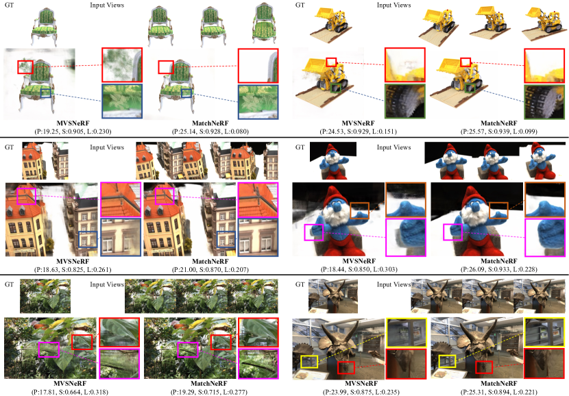
Figure 3: Qualitative results on Blender (1st row), DTU (2nd row) and RFF (3rd row). We showcase the visual results of MVSNeRF and our MatchNeRF method. Input views contain 3 viewpoints nearest to the target one, and the first input view is the reference view for MVSNeRF. Our MatchNeRF reconstructs better details (‘leaves’ scene of RFF) and contains less background artifacts (‘doll’ scene of DTU). The construction of cost volume in MVSNeRF requires all other views to be warped to the reference view, which results in poor quality when some views are clearly different from the reference view (‘chair’ scene of Blender, elaborated in Sec. A.1). Quantitative results measured over the whole image are placed below each image, which in order are scores of PSNR, SSIM and LPIPS.

4.1 Ablation Experiments

Model components. We evaluate the importance of different network components of our full model, reported in Tab. 1a. We start from a baseline with only CNN-based feature extractor (‘CNN’), which is commonly used in prior works [30, 8, 42, 6]. When adding a Transformer with only self-attention (‘CNN+self’), the performance only sees a small improvement. However, the model is significantly improved when the backbone features are refined with a cross-attention based Transformer (‘CNN+cross’), showing that it is critical to model cross-view interactions in feature extraction. We then use both self- and cross-attention to further enhance our backbone (‘CNN+self+cross’). Finally, we add a ray Transformer to our decoder to enhance the cross-point interactions along the ray space (‘CNN+self+cross+ray’), which brings additional improvements.

Feature relation measures. Another key component of our method is the explicitly modeled correspondence matching information, which is implemented with group-wise cosine similarity between sampled Transformer features. We compare with other potential counterparts in Tab. 1b to demonstrate the strength of our method. A straightforward option would be directly concatenating the features. However, its performance has a significant gap with our method even though Transformer features are also used, which indicates that pure stronger features are not very effective in providing direct guidance to the density prediction. SRF [8] proposes to implicitly learn the feature similarity with a network, instead of explicitly computing the similarity with the parameter-free cosine function as in our method. We implement SRF’s method by predicting a scalar output from two input features as the implicitly learned similarity. We can observe SRF’s approach is considerably worse, suggesting that our explicit cosine feature similarity is more effective. Next, we compare with the variance metric typically used in cost volume-based approaches like MVSNeRF [6], our group-wise cosine similarity again performs better. Compared with the basic cosine similarity that reduces two high dimensional features to a single scalar, which might lose too much information, our group-wise computation is more advantageous and thus leads to the best results.

Input	Method	DTU [13]			Real Forward-Facing [22]			Blender [22]
		PSNR$\uparrow$	SSIM$\uparrow$	LPIPS$\downarrow$	PSNR$\uparrow$	SSIM$\uparrow$	LPIPS$\downarrow$	PSNR$\uparrow$	SSIM$\uparrow$	LPIPS$\downarrow$
3-view	PixelNeRF [49]	19.31	0.789	0.382	11.24	0.486	0.671	7.39	0.658	0.411
	IBRNet [42]	26.04	0.917	0.190	21.79	0.786	0.279	22.44	0.874	0.195
	MVSNeRF [6]	26.63	0.931	0.168	21.93	0.795	0.252	23.62	0.897	0.176
	MatchNeRF	26.91	0.934	0.159	22.43	0.805	0.244	23.20	0.897	0.164
	MVSNeRF$\top$[6]	20.67	0.865	0.296	20.78	0.778	0.283	24.63	0.929	0.155
	MatchNeRF$\top$	24.54	0.897	0.257	21.77	0.795	0.276	24.65	0.930	0.120
2-view	MVSNeRF [6]	24.03	0.914	0.192	20.22	0.763	0.287	20.56	0.856	0.243
	MatchNeRF	25.03	0.919	0.181	20.59	0.775	0.276	20.57	0.864	0.200
	MVSNeRF$\top$[6]	19.08	0.831	0.340	18.13	0.730	0.345	21.68	0.875	0.216
	MatchNeRF$\top$	23.66	0.886	0.285	19.28	0.760	0.310	22.11	0.906	0.151

Table 2: Comparison with SOTA methods. MatchNeRF performs the best for both 3- and 2-view inputs. Viewpoints nearest to the target one are selected as input. By default we measure over only the foreground or central regions following MVSNeRF’s settings, while ^$\top$ indicates a more accurate metric by measuring over the whole image. Default 3-view results are borrowed from MVSNeRF’s paper. We measure MVSNeRF’s 3-view whole image results with its pretrained weight, and retrain with its released code to report 2-view results.

Number of Transformer blocks. We also verify the gain of stacking different numbers of Transformer blocks for the encoder. Our default model uses a stack of 6 Transformer blocks, where each block contains a self-attention and a cross-attention layer. Tab. 1c shows the results of stacking 0, 1, 3, 6 Transformer blocks, respectively. Our model observes notable improvement when augmented with 1 Transformer block. It sees better performance when stacked with more blocks, and reaches the best with 6 blocks.

Feature resolution. We extract features at both $1/8$ and $1/4$ resolutions, and we compare their effects in Tab. 1d. We observe that the $1/4$ resolution model performs better especially in terms of SSIM and LPIPS metrics. Combining both $1/8$ and $1/4$ resolution features leads to the best performance and thus is used in our final model.

4.2 Main Results

SOTA comparisons. We mainly compare MatchNeRF with three state-of-the-art generalizable NeRF models, namely PixelNeRF [49], IBRNet [42] and MVSNeRF [6], under few-view settings (3- and 2-view). Although GeoNeRF [14] is built upon MVSNeRF, its released model is trained with ground-truth DTU depth data and extra scenes from two other datasets, making fair comparisons difficult. Similarly, we do not compare with Point-NeRF [46] since it mainly improves the per-scene fine-tuning stage, but does not perform well in our focus of generalizable setting (further discussed in Sec. A.2). Generally, these MVSNeRF follow-up works share similar limitations, as they all rely on cost volume. We thus choose MVSNeRF, one of the most representative cost volume-based methods, to showcase the potential of our matching-based design.

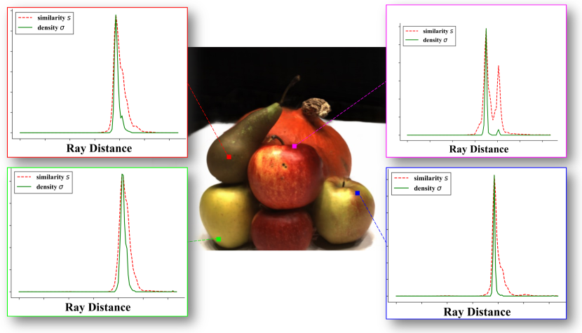
Figure 4: Relationship between the learned cosine similarity and volume density. Four pixels are randomly selected from the foreground of a DTU test scene (‘scan63’). For each pixel, we showcase the learned cosine similarity (scalar value, predicted by the ablation model ‘cosine’ in Tab. 1b) and volume density of all sampled points along the corresponding ray. The strong correlation demonstrates that our proposed cosine similarity is able to provide valuable geometric cues for volume density prediction.

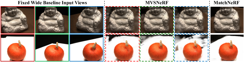
Figure 5: Visual results of using different reference views on DTU. Three fixed wide baseline views are used as input views. Each row presents the results of one target viewpoint from the corresponding test scene, and each image of MVSNeRF is rendered using the image with the same color border as the reference view. The visual quality of MVSNeRF becomes worse when the reference viewpoint is more different from the target one, especially around the background area. In contrast, our MatchNeRF is agnostic to the reference view.

Quantitative results in Tab. 2 show that our MatchNeRF performs the best in all datasets under the settings of both 3- and 2-view. By default we measure over only the foreground (DTU) or central (RFF and Blender) regions following the settings of MVSNeRF. Such settings are mainly introduced to ignore the background, as previous works emphasize more on the quality of only objects or scenes within small volumes, mostly due to the limitations of cost volume. Considering that the reconstruction of entire scenes are more practical and have drawn increasing attention recently [28, 35], it is undoubted that the background should also be included in measuring image quality, and thus it is more accurate to measure over the whole image. When reporting over the whole image (marked with ^$\top$ in Tab. 2), the advantage of MatchNeRF is glaringly obvious, showing that our method can render high-quality contents for both the foreground and background. Such a superiority can be more vividly observed from the visual results (Fig. 3). Notice that views rendered by MVSNeRF tend to contain artifacts around the background, since its cost volume is built towards one specific reference view, where the camera frustum might not have enough cover of the target view. Moreover, under the more challenging 2-view setting, MatchNeRF outperforms MVSNeRF by a larger margin, showing that our explicit correspondence matching provides more effective geometric cues for learning generalizable NeRF.

The main reason for the superiority of our model is that our encoder is able to provide a compact and effective hint about the geometry structure for the decoder, thus making the learning process easier. Although MatchNeRF operates in 2D feature space similar to PixelNeRF and IBRNet, it significantly outperforms these two methods, suggesting that our proposed cross-view-aware features do help the 3D estimation task. Our method also outperforms MVSNeRF that relies on 3D CNNs, indicating the effectiveness of our explicitly modeled correspondence matching information. Fig. 4 illustrates the strong correlation between the learned cosine similarity and volume density. We also show in the appendix that MatchNeRF excels at per-scene fine-tuning (Sec. A.2), reconstructs better depth (Sec. A.3) and benefits from extra input views (Sec. A.4).

Method	Ref.	PSNR$\uparrow$	SSIM$\uparrow$	LPIPS$\downarrow$
MVSNeRF$\top$[6]	1st	16.98	0.766	0.391
	2nd	17.87	0.787	0.375
	3rd	14.92	0.715	0.434
MatchNeRF$\top$	-	18.65	0.818	0.339

Table 3: Effect of selecting different reference views on DTU. Three fixed wide baseline views are used as input views. ‘Ref.’ states ID of the selected reference view. Results measured over the whole image show that MVSNeRF is sensitive to the selection of reference view, while our MatchNeRF is view-agnostic.

Effect of reference view selection. The above experiments follow MVSNeRF’s setting of choosing input views nearest to the target one, which again helps “hide” the limitations caused by the cost volume. Here we re-evaluate the models by using three fixed wide baseline input views to further demonstrate the superiority of our design. As shown in Fig. 5, the performance of MVSNeRF is highly sensitive to the selection of reference view, where the performance drops significantly when the selected reference view does not have sufficient overlap with the target one. In contrast, our MatchNeRF is by design view-agnostic, and achieves good performances even for the background regions. Quantitative results (see Tab. 3) measured over the whole image on all DTU test scenes further reassure our findings.

Method	Input	PSNR$\uparrow$	SSIM$\uparrow$	LPIPS$\downarrow$
IBRNet [42]	10-view	24.33	0.801	0.213
GPNR [32]	5-view	24.33	0.850	0.216
	3-view	22.36	0.800	0.286
MatchNeRF	3-view	24.82	0.860	0.214

Table 4: Comparisons on RFF following ‘GPNR Setting 1’[32]. Despite using only 3 input views, MatchNeRF performs the best compared to other methods that require 5 or even 10 input views.

Comparisons on GPNR Setting 1. Aiming to fairly compare with prior methods, we further validate MatchNeRF by adopting another popular configuration. We follow ‘GPNR Setting 1’ to train on LLFF [21] and IBRNet [42] collected scenes, and conduct generalization test on RFF [22] dataset. Readers are referred to GPNR [32] for more setting details.

As reported in Tab. 4, our MatchNeRF with only 3 input views is able to outperform IBRNet [42] with 10 input views in terms of PSNR and SSIM. MatchNeRF also showcases its superiority by achieving better performance than 3-view and even 5-view GPNR [32]. Note that GPNR [32] is trained on 32 TPUs whereas MatchNeRF is trained on only one single 16G-V100 GPU. This reassures us that explicit correspondence matching can provide reliable geometry cues, enabling generalizable NeRF models to generalize to unseen scenes in a more effective and efficient manner.

5 Conclusion

We have proposed a new generalizable NeRF method that uses explicit correspondence matching statistics as the geometry prior. We implemented the matching process by applying group-wise cosine similarity over pair-wise features that are enhanced with a cross-view Transformer. Different from the cost volume-based approaches that are inherently limited by the selection of the reference view, our matching-based design is view-agnostic. We showcased that our explicit correspondence matching information can provide valuable geometry cues for the estimation of volume density, leading to state-of-the-art performance under several challenging settings on three benchmarks datasets.

Appendix A More Experimental Analysis

A.1 Limitation of Cost Volume

To better understand the limitation of cost volume, we further visualize the warped input views in Fig. 6. The construction of cost volume relies on warping different input views to one selected reference view with different depth planes, where artifacts will be inevitably introduced in the background of those warped views. Thus, the quality of the cost volume is inherently limited, accordingly leading to artifacts in the background of the rendered image (see Fig. 3). In contrast, our method avoids the warping and cost volume construction operations, thus achieving better performance both qualitatively and quantitatively.

A.2 Per-scene Fine-tuning

Although MatchNeRF is designed for generalizing to new unseen scenes, it can also incorporate an additional per-scene fine-tuning stage. We follow the settings of MVSNeRF to fine tune our model on each specific DTU test scene with 16 additional training views. As reported in Tab. 5, MatchNeRF again outperforms its main competitor MVSNeRF under the same 10k iterations of per-scene fine-tuning, with a shorter optimization time (16-mins vs. 24-mins). Note that despite outstanding per-scene fine-tuning performance, Point-NeRF [46] ($23.89/0.874/0.203$) performs much worse than MVSNeRF($26.63/0.931/0.168$) and our MatchNeRF ($26.91/0.934/0.159$) under our main focus of generalizable setting.

A.3 Depth Reconstruction

We compare with state-of-the-art generalizable NeRF models regarding depth reconstruction (see Tab. 6), our MatchNeRF again achieves the best results. The main reason is that the depth map is rendered from the volume density (as it is done in NeRF [22]), and our matching-based encoder can provide reliable geometry cues for density prediction (see Fig. 4), thus leading to better reconstructed depth. Visual results presented in Fig. 7 further reassure our findings, notice that MatchNeRF reconstruct sharper and cleaner borders compared to MVSNeRF.

Figure 6: Illustration of warping two input views to the reference view with different depth planes. The construction of cost volume relies on warping different input views to the reference view with different depth planes, where inevitable artifacts will be introduced in the background due to the warping operation.

Methoditerations	PSNR$\uparrow$	SSIM$\uparrow$	LPIPS$\downarrow$	Time$\downarrow$
NeRF200k	27.01	0.902	0.263	10 hr
Point-NeRF10k	30.12	0.957	0.117	20 min
MVSNeRF10k	28.50	0.933	0.179	24 min
MatchNeRF10k	28.53	0.938	0.170	16 min

Table 5: Comparisons on DTU using per-scene fine-tuning setting. Despite outstanding results with fine-tuning, Point-NeRF is much worse than our MatchNeRF under our main focus of generalizable setting. The results of other models are all borrowed from Point-NeRF’s paper, measured over the foreground region.

Metric	PixelNeRF	IBRNet	MVSNeRF	Ours
Abs error$\downarrow$	0.239	1.62	0.035	0.032
Acc (0.05)$\uparrow$	0.187	0.001	0.866	0.886

Table 6: Depth reconstruction comparisons on DTU. ‘Abs error’ and ‘Acc (0.05)’ are short for absolute error and accuracy with a 0.05 threshold, respectively. Results are measured over the foreground as DTU has no ground-truth depth data for the background.

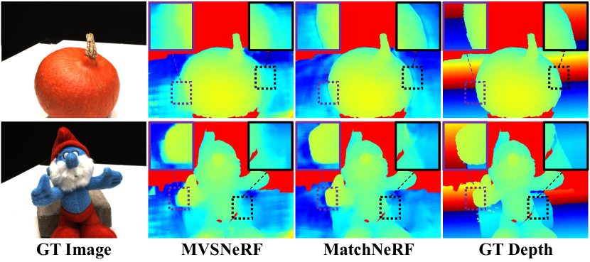
Figure 7: Visual results of rendered depth maps on DTU. Background regions are masked out for depth maps rendered by both methods since ground-truth values are not available for those regions. MatchNeRF reconstructs better depth with sharper borders.

A.4 More Input Views

Our MatchNeRF directly uses all input views by calculating matching similarity on pair-wise cross-view-aware features, thus it is by design able to capture more information when given more input views. As reported in Tab. 7, our MatchNeRF indeed achieves better performance with more input views. Besides, we also report the average inference time for each test batch (contains 4096 rays in our experiment). As expected, the runtime slightly increases as the number of views grows.

Input	PSNR$\uparrow$	SSIM$\uparrow$	LPIPS$\downarrow$	Runtime$\downarrow$
2-view	25.03	0.919	0.181	0.06 s
3-view	26.91	0.934	0.159	0.08 s
4-view	27.04	0.936	0.159	0.11 s
5-view	27.11	0.936	0.161	0.15 s
6-view	27.38	0.938	0.157	0.20 s

Table 7: MatchNeRF with varying input views on DTU. MatchNeRF can perform better when given more input views, but it also takes a longer runtime. The results are reported on DTU using nearest input views, measured over the foreground region. Runtime is measured over a test batch (4096-rays).

A.5 Backbone Training Strategy

As stated in Sec. 4, our feature extractor is initialized with GMFlow’s released weights. We observe that such a publicly available pretrained model can serve as a good initialization to our encoder, hence saving us time in training the full model. We further compare with other training strategies, so as to better demonstrate the effectiveness of our default model (Tab. 8 ‘pretrained + finetune’).

Is GMFlow’s released weights effective enough to be directly used (without any finetuning) in our task? NO. MatchNeRF performs poorly if we freeze the backbone initialized with the pretrained weights and train solely the NeRF decoder (Tab. 8 ‘pretrained + freeze’). The main reason is that GMFlow is trained on Sintel [3] for optical flow estimation, whose full model and final objective share little in common with ours. In particular, Sintel has no overlap with any data we used, and its contents are notably different from ours (video game scenes vs. daily life scenes). Moreover, MatchNeRF is built for novel view synthesis rather than optical flow estimation, the differences between these two tasks further reduce the effectiveness of GMFlow’s pretrained model. The key observation is that our backbone features should be aligned across different views, which does share similar objective with that of GMFlow’s backbone, thus its pretrained model can serve as a good initialization but requires further fine-tuning to adapt to our task.

Can our MatchNeRF be trained from scratch? YES. We retrain our MatchNeRF by randomly initializing the whole framework. As shown in Tab. 8, the ablation model (‘random init + finetune’) achieves comparable results with our default model, which again outperforms our main competitor MVSNeRF ($20.67/0.865/0.296$). It demonstrates that the cross-view interactions can be learned from scratch without any explicit correspondence supervision.

In general, our MatchNeRF can be trained from scratch to achieve state-of-the-art performance, and it can be further enhanced by leveraging the publicly available GMFlow pretrained model as an initialization.

Setting	PSNR$\uparrow$	SSIM$\uparrow$	LPIPS$\downarrow$
pretrained + freeze	20.36	0.845	0.318
random init + finetune	23.44	0.881	0.283
pretrained + finetune	24.54	0.897	0.257

Table 8: Backbone training strategy. The results are reported on DTU using 3 nearest input views, measured over the whole image. The settings ‘random init’ and ‘pretrained’ denote the backbone is ‘randomly initialized’ and ‘initialized with GMFlow pretrained weights’, respectively. The settings ‘freeze’ and ‘finetune’ refer to ‘freeze’ and ‘finetune’ the trainable parameters of the backbone, respectively. Although MatchNeRF can be trained from scratch to reach state-of-the-art performance, leveraging the publicly available pretrained weights as an initialization leads to better results.

A.6 Discussion

We acknowledge that our current architecture might be less effective at handling occlusions since they have not been explicitly modeled. These occlusion issues may become severe when the input contains a large number of views. Nonetheless, we reiterate that this work mainly focuses on the challenging yet practical few-view (e.g., 2 or 3) scenarios, and we believe that it can serve as a novel basis for further related research, e.g., enhancing it by explicitly modeling the occlusion factor.

Appendix B More Implementation Details

Multi-view feature extraction backbone. We follow the default setting of GMFlow [44] to compute feature attentions within local windows using the strategy of fixed number of local windows. In particular, the $8\times$ downsampled convolutional features ${\bm{F}}^{\mathrm{c}}$ with size $H\times W$ are split into $2\times 2$ local windows, each with size $\frac{H}{2}\times\frac{W}{2}$. The output feature dimension of the ‘Cross-View Transformer’ is 128. We refer readers to the supplementary document of GMFlow for more details about network architectures.

We further upsample the enhanced $1/8$ resolution Transformer feature ${\bm{F}}$ to the $1/4$ resolution $\hat{\bm{F}}$ with a lightweight CNN-based upsampler. Our feature upsampler is mainly adopted from the ‘Neural Rendering Operator’ introduced in GIRAFFE [25], except that our output feature dimension remains unchanged as 128 instead of reducing to 3.

NeRF decoder. Following a similar design of existing representative generalizable NeRF models [42, 6], our decoder operates in the input camera space instead of the general canonical space, since the former can discourage overfitting [37] and encourage better generalization to unseen scenes [30]. As illustrated in Fig. 8, our NeRF decoder takes as input the coordinate information (position ${\bm{p}}$ and direction ${\bm{d}}$) and the prior information (geometry prior ${\bm{z}}$ and texture prior ${\bm{\dot{}}{c}}$), where the latter is leveraged as a modulation and fed into each layer. Such a modulation-based design is inspired by SPADE [26] and has been successful in  [19, 49, 6]. Besides, we also follow MVSNeRF [6] and apply positional encoding only to ${\bm{p}}$ but not to ${\bm{d}}$. Our MLP has 6 layers and each layer has 128 dimensions. The ray Transformer is borrowed from IBRNett [42], mainly composed of a single multi-head self-attention [40] layer, and we refer readers to IBRNet’s supplement for further details.

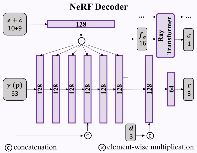
Figure 8: Architecture of the NeRF decoder. Input and output features are shown in gray blocks, where the numbers below denote the corresponding channel dimensions. Trainable linear layers are represented with purple blocks, where the numbers inside indicate the output channel dimensions. The ray Transformer is adopted from IBRNet [42], which takes as input the density features of all sampled points along the whole ray and outputs the corresponding density values. $\gamma$ is positional encoding, $\dot{c}$ is texture prior, other notations are the same as those in Sec. 3.

Training details. We uniformly sample 128 points for each rendering ray, and reconstruct only one single radiance field, without using the coarse-to-fine technique. 512 rays are randomly sampled in each training batch. The model is trained with AdamW [18] optimizer, and the learning rates are initialized as 5e-5 for the encoder and 5e-4 for the decoder, decayed using the one cycle policy [31]. We also clip the global norm of gradients of the cross-view Transformer to $\leqslant 1$ to avoid exploding gradients. Our MatchNeRF is implemented with PyTorch [27] and its default model is trained for 7 epochs, which takes around 28 hours on a single 16G-V100 GPU using the 3 input views settings.

References

- [1] Jonathan T Barron, Ben Mildenhall, Matthew Tancik, Peter Hedman, Ricardo Martin-Brualla, and Pratul P Srinivasan. Mip-nerf: A multiscale representation for anti-aliasing neural radiance fields. In ICCV, pages 5855–5864, 2021.
- [2] Jonathan T Barron, Ben Mildenhall, Dor Verbin, Pratul P Srinivasan, and Peter Hedman. Mip-nerf 360: Unbounded anti-aliased neural radiance fields. In CVPR, pages 5470–5479, 2022.
- [3] Daniel J Butler, Jonas Wulff, Garrett B Stanley, and Michael J Black. A naturalistic open source movie for optical flow evaluation. In ECCV, pages 611–625. Springer, 2012.
- [4] Nicolas Carion, Francisco Massa, Gabriel Synnaeve, Nicolas Usunier, Alexander Kirillov, and Sergey Zagoruyko. End-to-end object detection with transformers. In ECCV, pages 213–229. Springer, 2020.
- [5] Anpei Chen, Zexiang Xu, Andreas Geiger, Jingyi Yu, and Hao Su. Tensorf: Tensorial radiance fields. In ECCV, 2022.
- [6] Anpei Chen, Zexiang Xu, Fuqiang Zhao, Xiaoshuai Zhang, Fanbo Xiang, Jingyi Yu, and Hao Su. Mvsnerf: Fast generalizable radiance field reconstruction from multi-view stereo. In ICCV, pages 14124–14133, 2021.
- [7] Di Chen, Yu Liu, Lianghua Huang, Bin Wang, and Pan Pan. Geoaug: Data augmentation for few-shot nerf with geometry constraints. In ECCV, pages 322–337. Springer, 2022.
- [8] Julian Chibane, Aayush Bansal, Verica Lazova, and Gerard Pons-Moll. Stereo radiance fields (srf): Learning view synthesis for sparse views of novel scenes. In CVPR, pages 7911–7920, 2021.
- [9] Kangle Deng, Andrew Liu, Jun-Yan Zhu, and Deva Ramanan. Depth-supervised nerf: Fewer views and faster training for free. In CVPR, pages 12882–12891, 2022.
- [10] Xiaodong Gu, Zhiwen Fan, Siyu Zhu, Zuozhuo Dai, Feitong Tan, and Ping Tan. Cascade cost volume for high-resolution multi-view stereo and stereo matching. In CVPR, pages 2495–2504, 2020.
- [11] Xiaoyang Guo, Kai Yang, Wukui Yang, Xiaogang Wang, and Hongsheng Li. Group-wise correlation stereo network. In CVPR, pages 3273–3282, 2019.
- [12] Ajay Jain, Matthew Tancik, and Pieter Abbeel. Putting nerf on a diet: Semantically consistent few-shot view synthesis. In ICCV, pages 5885–5894, 2021.
- [13] Rasmus Jensen, Anders Dahl, George Vogiatzis, Engin Tola, and Henrik Aanæs. Large scale multi-view stereopsis evaluation. In CVPR, pages 406–413, 2014.
- [14] Mohammad Mahdi Johari, Yann Lepoittevin, and François Fleuret. Geonerf: Generalizing nerf with geometry priors. In CVPR, pages 18365–18375, 2022.
- [15] James T Kajiya and Brian P Von Herzen. Ray tracing volume densities. ACM TOG, 18(3):165–174, 1984.
- [16] Yuan Liu, Sida Peng, Lingjie Liu, Qianqian Wang, Peng Wang, Christian Theobalt, Xiaowei Zhou, and Wenping Wang. Neural rays for occlusion-aware image-based rendering. In CVPR, pages 7824–7833, 2022.
- [17] Ze Liu, Yutong Lin, Yue Cao, Han Hu, Yixuan Wei, Zheng Zhang, Stephen Lin, and Baining Guo. Swin transformer: Hierarchical vision transformer using shifted windows. In ICCV, pages 10012–10022, 2021.
- [18] Ilya Loshchilov and Frank Hutter. Decoupled weight decay regularization. In ICLR, 2019.
- [19] Lars Mescheder, Michael Oechsle, Michael Niemeyer, Sebastian Nowozin, and Andreas Geiger. Occupancy networks: Learning 3d reconstruction in function space. In CVPR, pages 4460–4470, 2019.
- [20] Ben Mildenhall, Peter Hedman, Ricardo Martin-Brualla, Pratul P Srinivasan, and Jonathan T Barron. Nerf in the dark: High dynamic range view synthesis from noisy raw images. In CVPR, pages 16190–16199, 2022.
- [21] Ben Mildenhall, Pratul P Srinivasan, Rodrigo Ortiz-Cayon, Nima Khademi Kalantari, Ravi Ramamoorthi, Ren Ng, and Abhishek Kar. Local light field fusion: Practical view synthesis with prescriptive sampling guidelines. ACM TOG, 38(4):1–14, 2019.
- [22] Ben Mildenhall, Pratul P. Srinivasan, Matthew Tancik, Jonathan T. Barron, Ravi Ramamoorthi, and Ren Ng. Nerf: Representing scenes as neural radiance fields for view synthesis. In ECCV, pages 405–421, 2020.
- [23] Thomas Müller, Alex Evans, Christoph Schied, and Alexander Keller. Instant neural graphics primitives with a multiresolution hash encoding. ACM TOG, 41(4):102:1–102:15, July 2022.
- [24] Michael Niemeyer, Jonathan T. Barron, Ben Mildenhall, Mehdi S. M. Sajjadi, Andreas Geiger, and Noha Radwan. Regnerf: Regularizing neural radiance fields for view synthesis from sparse inputs. In CVPR, 2022.
- [25] Michael Niemeyer and Andreas Geiger. Giraffe: Representing scenes as compositional generative neural feature fields. In CVPR, pages 11453–11464, 2021.
- [26] Taesung Park, Ming-Yu Liu, Ting-Chun Wang, and Jun-Yan Zhu. Semantic image synthesis with spatially-adaptive normalization. In CVPR, pages 2337–2346, 2019.
- [27] Adam Paszke, Sam Gross, Francisco Massa, Adam Lerer, James Bradbury, Gregory Chanan, Trevor Killeen, Zeming Lin, Natalia Gimelshein, Luca Antiga, et al. Pytorch: An imperative style, high-performance deep learning library. NeurIPS, 32, 2019.
- [28] Christian Reiser, Richard Szeliski, Dor Verbin, Pratul P Srinivasan, Ben Mildenhall, Andreas Geiger, Jonathan T Barron, and Peter Hedman. Merf: Memory-efficient radiance fields for real-time view synthesis in unbounded scenes. arXiv preprint arXiv:2302.12249, 2023.
- [29] Jeremy Reizenstein, Roman Shapovalov, Philipp Henzler, Luca Sbordone, Patrick Labatut, and David Novotny. Common objects in 3d: Large-scale learning and evaluation of real-life 3d category reconstruction. In ICCV, pages 10901–10911, 2021.
- [30] Daeyun Shin, Charless C Fowlkes, and Derek Hoiem. Pixels, voxels, and views: A study of shape representations for single view 3d object shape prediction. In CVPR, pages 3061–3069, 2018.
- [31] Leslie N Smith and Nicholay Topin. Super-convergence: Very fast training of neural networks using large learning rates. In Artificial intelligence and machine learning for multi-domain operations applications, volume 11006, pages 369–386. SPIE, 2019.
- [32] Mohammed Suhail, Carlos Esteves, Leonid Sigal, and Ameesh Makadia. Generalizable patch-based neural rendering. In ECCV. Springer, 2022.
- [33] Cheng Sun, Min Sun, and Hwann-Tzong Chen. Direct voxel grid optimization: Super-fast convergence for radiance fields reconstruction. In CVPR, 2022.
- [34] Mukund Varma T, Peihao Wang, Xuxi Chen, Tianlong Chen, Subhashini Venugopalan, and Zhangyang Wang. Is attention all that neRF needs? In ICLR, 2023.
- [35] Matthew Tancik, Vincent Casser, Xinchen Yan, Sabeek Pradhan, Ben Mildenhall, Pratul P Srinivasan, Jonathan T Barron, and Henrik Kretzschmar. Block-nerf: Scalable large scene neural view synthesis. In CVPR, pages 8248–8258, 2022.
- [36] Jiaxiang Tang, Xiaokang Chen, Jingbo Wang, and Gang Zeng. Compressible-composable nerf via rank-residual decomposition. NeurIPS, 2022.
- [37] Maxim Tatarchenko, Stephan R Richter, René Ranftl, Zhuwen Li, Vladlen Koltun, and Thomas Brox. What do single-view 3d reconstruction networks learn? In CVPR, pages 3405–3414, 2019.
- [38] Alex Trevithick and Bo Yang. Grf: Learning a general radiance field for 3d representation and rendering. In ICCV, pages 15182–15192, 2021.
- [39] Prune Truong, Marie-Julie Rakotosaona, Fabian Manhardt, and Federico Tombari. Sparf: Neural radiance fields from sparse and noisy poses. arXiv preprint arXiv:2211.11738, 2022.
- [40] Ashish Vaswani, Noam Shazeer, Niki Parmar, Jakob Uszkoreit, Llion Jones, Aidan N Gomez, Łukasz Kaiser, and Illia Polosukhin. Attention is all you need. NeurIPS, 30, 2017.
- [41] Dor Verbin, Peter Hedman, Ben Mildenhall, Todd Zickler, Jonathan T Barron, and Pratul P Srinivasan. Ref-nerf: Structured view-dependent appearance for neural radiance fields. In CVPR, pages 5481–5490. IEEE, 2022.
- [42] Qianqian Wang, Zhicheng Wang, Kyle Genova, Pratul P Srinivasan, Howard Zhou, Jonathan T Barron, Ricardo Martin-Brualla, Noah Snavely, and Thomas Funkhouser. Ibrnet: Learning multi-view image-based rendering. In CVPR, pages 4690–4699, 2021.
- [43] Zhou Wang, Alan C Bovik, Hamid R Sheikh, and Eero P Simoncelli. Image quality assessment: from error visibility to structural similarity. IEEE TIP, 13(4):600–612, 2004.
- [44] Haofei Xu, Jing Zhang, Jianfei Cai, Hamid Rezatofighi, and Dacheng Tao. Gmflow: Learning optical flow via global matching. In CVPR, pages 8121–8130, 2022.
- [45] Qingshan Xu and Wenbing Tao. Learning inverse depth regression for multi-view stereo with correlation cost volume. In AAAI, volume 34, pages 12508–12515, 2020.
- [46] Qiangeng Xu, Zexiang Xu, Julien Philip, Sai Bi, Zhixin Shu, Kalyan Sunkavalli, and Ulrich Neumann. Point-nerf: Point-based neural radiance fields. In CVPR, pages 5438–5448, 2022.
- [47] Yao Yao, Zixin Luo, Shiwei Li, Tian Fang, and Long Quan. Mvsnet: Depth inference for unstructured multi-view stereo. In ECCV, pages 767–783, 2018.
- [48] Alex Yu, Ruilong Li, Matthew Tancik, Hao Li, Ren Ng, and Angjoo Kanazawa. Plenoctrees for real-time rendering of neural radiance fields. In ICCV, pages 5752–5761, 2021.
- [49] Alex Yu, Vickie Ye, Matthew Tancik, and Angjoo Kanazawa. pixelnerf: Neural radiance fields from one or few images. In CVPR, pages 4578–4587, 2021.
- [50] Zehao Yu, Songyou Peng, Michael Niemeyer, Torsten Sattler, and Andreas Geiger. Monosdf: Exploring monocular geometric cues for neural implicit surface reconstruction. NeurIPS, 2022.
- [51] Richard Zhang, Phillip Isola, Alexei A Efros, Eli Shechtman, and Oliver Wang. The unreasonable effectiveness of deep features as a perceptual metric. In CVPR, pages 586–595, 2018.