Joint Message Detection and Channel Estimation for Unsourced Random Access in Cell-Free User-Centric Wireless Networks

Abstract

We consider unsourced random access (uRA) in a cell-free (CF) user-centric wireless network, where a large number of potential users compete for a random access slot, while only a finite subset is active. The random access users transmit codewords of length $L$ symbols from a shared codebook, which are received by $B$ geographically distributed radio units (RUs) equipped with $M$ antennas each. Our goal is to devise and analyze a centralized decoder to detect the transmitted messages (without prior knowledge of the active users) and estimate the corresponding channel state information. A specific challenge lies in the fact that, due to the geographically distributed nature of the CF network, there is no fixed correspondence between codewords and large-scale fading coefficients (LSFCs). This makes current “activity detection” approaches which make use of this fixed LSFC-codeword association not directly applicable. To overcome this problem, we propose a scheme where the access codebook is partitioned in “location-based” subcodes, such that users in a particular location make use of the corresponding subcode. The joint message detection and channel estimation is obtained via a novel Approximated Message Passing (AMP) algorithm to estimate the linear superposition of matrix-valued "sources" corrupted by Gaussian noise. The matrices to be estimated exhibit zero rows for inactive messages and Gaussian-distributed rows corresponding to the active messages. The asymmetry in the LSFCs and message activity probabilities leads to different statistics for the matrix sources, which distinguishes the AMP formulation from previous cases.In the regime where the codebook size scales linearly with $L$, while $B$ and $M$ are fixed, we present a rigorous high-dimensional analysis of the proposed AMP algorithm. Then, exploiting the fundamental decoupling principle of AMP, we provide a comprehensive analysis of Neyman-Pearson message detection, along with the subsequent channel estimation. The resulting system allows the seamless formation of user-centric clusters and very low latency beamformed uplink-downlink communication without explicit user-RU association, pilot allocation, and power control. This makes the proposed scheme highly appealing for low-latency random access communications in CF networks.

Keywords— Unsourced random access, cell-free user-centric networks, Approximated Message Passing (AMP), decoupling principle, Neyman-Pearson detection, low-latency communication.

1 Introduction

Multiuser multiple-input multiple-output (MU-MIMO) has been widely studied from an information theoretic point of view [1, 2, 3, 4] and has become an important component of the physical layer of cellular systems [5, 6] and wireless local area networks (see [7, 8] and references therein). As a further extension of MU-MIMO, joint processing of spatially distributed remote radio units (RUs), which can be traced back to [9], has been studied in different contexts and under different names such as coordinate multipoint, cloud radio access network, or cell-free (CF) MIMO. [10, 11, 12, 13, 14, 15, 16]. In this paper we focus on user-centric architectures as defined in [15], where each user is served by a localized cluster of nearby RUs, and each RU in turn serves a limited set of nearby users.

A crucial aspect enabling spatial multiplexing is the availability of channel state information at the infrastructure side (i.e., base stations, RUs) in order to enable multiuser detection in the uplink (UL) and multiuser precoding in the downlink (DL). In particular, channel state information for the DL is obtained by exploiting the UL/DL channel reciprocity, which holds under mild conditions in Time Division Duplexing (TDD) systems [17, 6]. Presently, most works on CF MIMO assumes that transmission resources (e.g., UL pilot sequences, time-frequency slots, and user-centric RU clusters) are permanently assigned to all users in the system.

However, in highly dense scenarios, a static allocation of transmission resources would be impractical and highly inefficient due to the sporadic and intermittent activity exhibited by users. For such high-density systems, it is necessary to design a dynamic random access mechanism that allows users to access the system and request transmission resources only when they become active.

We assume that all RUs periodically broadcast a “clear to send” signal followed by a random access channel (RACH) slot where users can transmit a random access message (see Fig. 1). At the end of the RACH slot, the system must: 1) decode the random access messages and estimate the corresponding channel vectors; 2) associate to each decoded message a cluster of RUs for further allocated communication; 3) possibly decode a larger UL payload in a subsequent slot; 4) send a DL message which may just contain the requested content by the random access users and/or an acknowledgement possibly containing resource allocation information (assigned UL and DL slots, pilot sequences, transmit power) for further communication, in a typical packet-reservation multiple access (PRMA) scheme (e.g., see [18]). Without going into unnecessary details, in this paper we are concerned with the basic access protocol functions, namely: joint random access message detection and channel estimation, seamless cluster formation, and ultra-low latency beamformed DL response, which for brevity will be referred to as ACK message in the following.

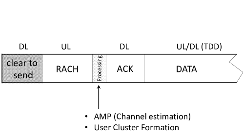
Figure 1: A schematic of the RACH slot, followed by a DL packet (referred to as ACK in this paper) and subsequent UL/DL TDD slots for allocated traffic.

Since assigning individual access codes to each user in advance is either impossible or highly impractical, it becomes necessary for all users to share the same access codebook. At the end of the RACH slot, the system must generate a list of collectively transmitted messages by the random access users, along with an estimation of the corresponding channel coefficient vectors. Even though the system may not yet know the identity of each random access user, it acknowledges that a user transmitting a certain $n$-th message in the detected list is requesting access and is associated with a channel estimate. Using this estimate, the system selects the set of $Q$ Resource Units (RUs) with the largest channel magnitudes (where $Q$ is a suitable system parameter) and transmits an ACK message using some form of DL precoding (e.g., Maximal-Ratio Transmission (MRT), as in [10]). Essentially, the random access messages act as "tokens," implicitly identifying the requesting users and their channel coefficients, and potentially encoding some additional information (e.g., the number of requested TDD slots for subsequent allocated communication).

1.1 Related literature on uRA

In current cellular systems, random access is a common practice [19] and works effectively when the number of random access users per RACH slot is small and there is a clear user-cell association, i.e., cell boundaries are clearly defined by the relative strength of cell-dependent beacon signals transmitted by each base station. However, in highly dense CF systems like the one described above, insisting on conventional schemes where each RU acts as a small base station quickly leads to highly congested situations. On the other hand, motivated by “Internet of Things” applications, random access from a huge population of users with very sporadic activity and using the same codebook, commonly referred to as unsourced Random Access (uRA), was proposed as an information-theoretic problem in [20] and it has been intensively investigated in recent years (e.g., [21, 22, 23, 24, 25]). In uRA, the receiver’s task is to decode the list of active messages, i.e., the list of codewords present in the noisy superposition forming the received signal, without knowing a priori which user is transmitting. Since all users share the same codebook, the total number of users in the system can be arbitrarily large, as long as the number of active messages in each RACH slot is finite. This property makes the uRA setting well-suited to the random access problem at hand.

The uRA setting bears strong similarities with the activity detection (AD) problem [26, 27, 28]. In AD, each user is given a unique signature sequence, and the receiver aims to identify the list of active users. Simply put, ”user” in activity detection plays the role of ”message” in uRA. However, it is important to note an important difference: in AD there is a fixed association between a user’s signature sequence and its set of large-scale fading coefficients (LSFCs), which describe the channel attenuation between the user and the RUs. In the uRA, there is no such fixed association between codewords and LSFCs, since any message can be transmitted by any user at any location within the coverage area.

Various works have addressed the AD problem for multiantenna receivers. Notably, the so-called multiple-measurement vector approximate message passing algorithm [29, 30, 31] (MMV-AMP, for short) is used in [26, 27, 28], the covariance-based algorithm in [23] (also analyzed in [32]), and the tensor-based modulation scheme in [33] are well-known and widely studied approaches. In particular, [23] shows that AMP performs well in the linear regime, where the signature block length $L$ scales linearly with the number of active users, and the number of antennas at the receiver $M$ is constant and typically small compared to $L$. In contrast, the covariance-based method achieves low activity detection error probability in the quadratic regime, where the number of active users scales as $L^{2}$, and the number of antennas $M$ scales slightly faster than $L^{2}$.

Numerous works have followed [28, 23], and providing a comprehensive account here would be impractical. Notably, some recent papers have focused on the activity detection problem in CF systems. For instance, [34] proposes a heuristic “distributed” AMP algorithm independently computed at each RU, followed by pooling the results for centralized detection of active users. In concurrent work, [35] considers a “centralized” AMP approach where observations from all RUs are jointly processed. It is important to note that both approaches lack a rigorous analysis. In this contribution, we propose a centralized AMP algorithm based on the idea of location-based partitioned codebook, that we outline in the sequel, and provide a rigorous high-dimensional analysis of the AMP concentration and asymptotic output statistics. This provides an analytical handle analyze in almost-closed form the message detection, the channel estimation, and the achievable rate in the ACK slot.

The covariance-based approach for the multi-cell case is considered in [36, 37, 38]. However, this approach is only competitive in the aforementioned quadratic regime, where channel vectors associated with active messages cannot be estimated. In the considered RACH scheme, channel estimates for active messages play a crucial role in fast user-centric cluster formation and beamformed ACK. Therefore, in this work, we focus on the linear scaling regime (i.e., the access codebook size scales linearly with the block length $L$), and we concentrate on the analysis of centralized AMP.

1.2 Contributions

To overcome the challenge of the unknown association between LSFCs and access codewords, we propose a “location-based” approach: the coverage area ${\cal D}$ is partitioned into $U$ regions $\{{\cal L}_{u}:u\in[U]\}$ referred to as “locations”, where $U$ is some suitable integer. The locations are designed such that the users within each location ${\cal L}_{u}$ experience similar LSFC profiles. The common random access codebook is partition into location-based subcodes, and users in a given location ${\cal L}_{u}$ are restricted to use the codewords of the associated $u$-th subcode. Hence, the scheme allows general statistical asymmetry between users in different locations, but enforces statistical symmetry between users within the same location. It should be noticed that also conventional cellular systems use a “location based” approach, where a one-to-one correspondence between locations and cells is enforced. Hence, our approach can be seen as the generalization of a somehow conventional approach to the CF case (e.g., see also [39] for a location-based approach to beam alignment in mmWave CF networks). For the above model, we propose an AMP algorithm that takes into account the statistical asymmetries across locations.

Our main theoretical contribution is the rigorous high-dimensional analysis of this new AMP algorithm. We also establish the asymptotic consistency of the decoupling principles manifested in the AMP analysis and the replica-symmetric (RS) computation of the static problem. Crucially, this implies that the proposed AMP algorithm asymptotically achieves the Bayesian optimality under the validity of the RS approach.

Exploiting the fundamental decoupling principle of AMP, we provide (rigorous) analysis of Neyman-Pearson type message detection and the subsequent channel estimation.

In closing, we provide several useful insights related to the beamformed ACK transmission in the DL, showing the effectiveness of the proposed scheme for uRA with seamless connectivity and short latency in CF networks.

1.3 Organization

The paper is organized as follows: In Section 2, we introduce the system model and the problem definition. Section 3 presents our main theoretical results. As applications of these results, Section 4 delves into the analyses of the Neyman-Pearson type detection algorithm and the subsequent channel estimation phase. In Section 5, we discuss cluster formation and beamformed ACH transmission. Simulation results are presented in Section 6. We conclude the paper in Section 7. The proofs are given in the Appendix.

1.4 Notations

We use the index set notation $[N]\stackrel{{\scriptstyle\Delta}}{{=}}\{1,\ldots,N\}$. Row vectors, column vectors, and matrices are denoted by boldfaced lower case letters, underlined bold-faced lower case letters, and boldfaced upper case letters, respectively (e.g., ${\bf a}$, $\underline{{\bf a}}$, and ${\bf A}$). The $i$th row and the $j$th column of ${\bf A}$ are denoted by ${{\bf a}}_{i}$ and ${\underline{{\bf a}}}_{j}$, respectively. We use ${\bf A}>\bf 0$ (resp. ${\bf A}\geq\bf 0$) to indicate that ${\bf A}$ is positive definite (resp. positive semi-definite), $(\cdot)^{\sf T}$ and $(\cdot)^{\sf H}$ to denote transpose and Hermitian transpose, and $\otimes$ to indicate the Kronecker product. Also, ${\bf I}_{m}$ indicates the $m\times m$ identity matrix. We denote the Frobenious norm of a matrix ${\bf A}$ by $\|{\bf A}\|_{\rm F}\stackrel{{\scriptstyle\Delta}}{{=}}\sqrt{{\hbox{tr}}({\bf A}^{\sf H}{\bf A})}$. We use the Matlab-like notation for which ${\hbox{diag}}({\bf a})$ or ${\hbox{diag}}(\underline{{\bf a}})$ is a diagonal matrix with diagonal elements defined by the corresponding vector argument, and ${\rm diag}({\bf A})$ returns a column vector of the diagonal elements of ${\bf A}$. The multivariate circularly-symmetric complex Gaussian distribution with mean ${\bf m}$ and covariance ${\bf C}$ is denoted by $\mathcal{CN}({\bf m},{\bf C})$. The Bernoulli distribution with mean $\lambda$ is denoted by ${\rm Bern}(\lambda)$. We write ${\bf a}\sim P$ to indicate that the random vector ${\bf a}$ has a probability distribution $P$. We use the notation ${\bf A}\sim_{\text{i.i.d.}}{{\bf a}}$ to indicate that the rows of the matrix ${\bf A}$ are independently and identically distributed (i.i.d.) copies of the random vector ${\bf a}$. Similarly, ${\bf A}\sim_{\text{i.i.d.}}P$ indicates that the rows of ${\bf A}$ are i.i.d. and have the probability distribution $P$. $\mathbb{E}[\cdot]$ indicates the expectation with respect to the joint distribution of all the random variables appearing in the argument. Finally, for a random matrix ${\bf A}$ (in general), we define $\|{\bf A}\|_{\mathcal{L}^{p}}\stackrel{{\scriptstyle\Delta}}{{=}}(\mathbb{E}[\|{\bf A}\|_{\rm F}^{p}])^{\frac{1}{p}}$ for $p\geq 1$, i.e., the $\mathcal{L}^{p}$-norm of the random variable $\|{\bf A}\|_{\rm F}$.

2 System Model and Problem Definition

Consider a CF wireless network with $B$ radio units (RUs) with $M$ antennas each, and a very large number of users geographically distributed in a certain coverage area ${\cal D}$. In order to overcome the problem of the association between codewords and LSFCs, we propose a location-based uRA approach, illustrated by the “toy example” of Fig. 2.

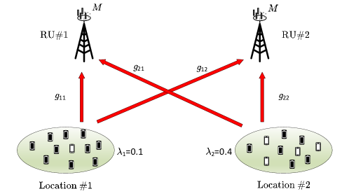
Figure 2: A simple $B=2$, $U=2$ toy model example of the proposed location-based approach.

The coverage area ${\cal D}$ is partitioned into $U$ zones, referred to as locations and denoted by ${\cal L}_{1},\ldots,{\cal L}_{U}$, such that the users in any given location have the same LSFC profile to all the RUs. In particular, we define the location-dependent nominal LSFC profile $\{g_{u,b}:b\in[B]\}$ for location ${\cal L}_{u}$, and assume that the LSFCs of all users in ${\cal L}_{u}$ to RU $b$ are equal to $g_{u,b}$. In reality, users are not perfectly co-located and the actual LSFCs will (slightly) differ from the nominal ones. We shall develop the detection algorithm under the matched assumption (real $=$ nominal). Our analysis holds also in the mismatched case (real $\approx$ nominal) and can be used to precisely quantify the degradation incurred by this mismatch. However, we leave the quantification of the mismatched effect for relevant geometries and pathloss models to a future follow-up paper, oriented specifically to “practical” wireless communication aspects.

Following [20, 21, 22, 23, 24, 25], an uRA codebook of block length $L$ and size $N$ is formed by a set of $N$ codewords arranged as the columns of a matrix ${\bf S}\in\mbox{\bb C}^{L\times N}$. With our location-based scheme, the codebook ${\bf S}$ is partitioned into $U$ subcodes, i.e., ${\bf S}=[{\bf S}_{1},\ldots,{\bf S}_{U}]$ such that ${\bf S}_{u}\in\mbox{\bb C}^{L\times N_{u}}$ and $\sum_{u}N_{u}=N$. The random access users in location ${\cal L}_{u}$ are aware of their location and make use of the corresponding codebook ${\bf S}_{u}$, i.e., any such user in order to transmit message $n\in[N_{u}]$, sends the corresponding codeword $\underline{{\bf s}}_{u,n}$ (i.e., the $n$-th column of ${\bf S}_{u}$). We assume that each codeword of ${\bf S}_{u}$ may be chosen independently with probability $\lambda_{u}\in(0,1)$, where $\lambda_{u}$ reflects the random activity of users in location ${\cal L}_{u}$.

The small scale fading coefficients between any user and any RU antenna are i.i.d. $\sim{\cal C}{\cal N}(0,1)$ RVs (independent Rayleigh fading), such that the channel vector between a user in ${\cal L}_{u}$ and the $M$-antenna array of RU $b$ is $\sim{\cal C}{\cal N}({\bf 0},g_{u,b}{\bf I}_{M})$. Consequently, the aggregated channel vector from a user in ${\cal L}_{u}$ to the $F\stackrel{{\scriptstyle\Delta}}{{=}}BM$ antennas of the RUs is a $1\times F$ Gaussian vector distributed as

$${\bf h}_{u}=[{\bf h}_{u,1},{\bf h}_{u,2},\ldots,{\bf h}_{u,B}]\sim{\cal C}{\cal N}({\bf 0},\hbox{\boldmath$\Sigma$}_{u}),$$ (1)

where $\hbox{\boldmath$\Sigma$}_{u}$ is a $F\times F$ diagonal matrix given by

$$\hbox{\boldmath$\Sigma$}_{u}={\rm diag}(g_{u,1},g_{u,2},\cdots,g_{u,B})\otimes{\bf I}_{M}\;.$$ (2)

The signal collectively received at the $F$ RUs antennas over the $L$ symbols of the RACH slot is given by the $L\times F$ (time-space) matrix

$${\bf Y} = \sum_{u=1}^{U}{\bf S}_{u}{\bf X}_{u}+{\bf W},$$ (3)

where ${\bf W}\sim_{\text{i.i.d.}}\mathcal{CN}({\mathchoice{\mbox{\boldmath$\displaystyle 0$}}{\mbox{\boldmath$\textstyle 0$}}{\mbox{\boldmath$\scriptstyle 0$}}{\mbox{\boldmath$\scriptscriptstyle 0$}}},\sigma_{w}^{2}{\bf I})$ is the additive white Gaussian noise and ${\bf X}_{u}\in\mbox{\bb C}^{N_{u}\times F}$ is the matrix containing (arranged by rows) the aggregate channel vectors corresponding to messages at location ${\cal L}_{u}$ to the receiving antennas. If the $n$-th message is not active (i.e., not transmitted), then the $n$-th row ${\bf x}_{u,n}$ of ${\bf X}_{u}$ is identically zero. If the $n$-th message is active (i.e., trasmitted), then ${\bf x}_{u,n}\sim{\bf h}_{u}$ (see (1)). Hence, we have ${\bf X}_{u}\sim_{\text{i.i.d.}}{\bf x}_{u}$, where ${\bf x}_{u}$ is the Bernoulli-Gaussian random vector

$${\bf x}_{u}\sim{a}_{u}{\bf h}_{u}\;,$$ (4)

with ${a}_{u}\sim{\rm Bern}(\lambda_{u})$ and ${\bf h}_{u}\sim\mathcal{CN}({\mathchoice{\mbox{\boldmath$\displaystyle 0$}}{\mbox{\boldmath$\textstyle 0$}}{\mbox{\boldmath$\scriptstyle 0$}}{\mbox{\boldmath$\scriptscriptstyle 0$}}},\hbox{\boldmath$\Sigma$}_{u})$, mutually independent.

We consider a random coding ensemble where each ${\bf s}_{u,n}\in\mbox{\bb C}^{L}$ is generated with i.i.d. elements $\sim{\cal C}{\cal N}(0,1/L)$. Defining the UL signal-to-noise ratio ${\sf SNR}$ as the average transmitted signal energy per symbol (for any active message) over the noise variance per component, the relation between ${\sf SNR}$ and $\sigma^{2}_{w}$ is $\sigma_{w}^{2}=1/(L{\sf SNR})$ (see Remark 5 in Section 5 on SNR normalization).

For each $u\in[U]$, let $\tilde{N}_{u}$ denote the random number (binomial $(\lambda_{u},N_{u})$ distributed) of active messages at location $u$ and let ${\bf P}_{u}\in\{0,1\}^{\tilde{N}_{u}\times N_{u}}$ denotes a "fat" projection matrix that eliminates zero-rows from the input signal ${\bf X}_{u}$. Then, we introduce

$$\underline{{\bf a}}_{u} \stackrel{{\scriptstyle\Delta}}{{=}}{\rm diag}({\bf P}_{u}^{\top}{\bf P}_{u})~{}~{}~{}\text{(True Message Activity Vector)}$$ (5)

$${\bf H}_{u} \stackrel{{\scriptstyle\Delta}}{{=}}{\bf P}_{u}{\bf X}_{u}~{}~{}~{}~{}~{}~{}~{}~{}~{}~{}~{}\text{(True Channel Matrix)}\;.$$ (6)

The goal of the a joint message detection and channel estimation algorithm is to recover the list of active messages (i.e., the binary vectors $\underline{{\bf a}}_{u}$) and estimate the corresponding channels ${\bf H}_{u}$ for each $u\in[U]$.

In view of its potential applicability to a wider range of applications, we consider the following generalization of input matrices: for all $u\in[U]$, let ${\bf X}_{u}\sim_{\text{i.i.d.}}{\bf x}_{u}$ for an arbitrary (and independent for each $u\in[U])$ random vector such that for all $p\in\mbox{\bb N}$ there exist a constant $C_{p}$ with

$$\|{\bf x}_{u}\|_{\mathcal{L}^{p}}\leq C_{p}\;.$$ (7)

If ${\bf x}_{u}$ is as in (4), then ${a}\stackrel{{\scriptstyle\Delta}}{{=}}\|{\bf x}\|$ is a sub-Gaussian RV, i.e., there exists a constant $C$ such that $\|{a}\|_{\mathcal{L}^{p}}\leq C\sqrt{p}$ for all $p\in\mbox{\bb N}$ [40]. In fact, for any large (constant) $D>0$ and a sub-Gaussian RV $a$, the RV $a^{D}$ satisfies the $\mathcal{L}^{p}$-norm bound as in (7). Namely, the family of RVs satisfying the $\mathcal{L}^{p}$-norm bounds as in (7) includes a wide range of distributions characterized by "heavy" exponential tails.

Let us formally outline the probabilistic model assumptions of and delineate the scaling parameters in our theoretical analysis:

Assumption 1.

Consider the observation model (3). Let the matrices in $\{\{{\bf S}_{u},{\bf X}_{u}\}_{u\in[U]},{\bf W}\}$ are mutually independent. For all $u\in[U]$, let ${\bf X}_{u}\sim_{\text{i.i.d.}}{\bf x}_{u}$ for some arbitrary random vector ${\bf x}_{u}\in\mbox{\bb C}^{F}$ satisfying (7). Also, let ${\bf W}\sim_{\text{i.i.d.}}\mathcal{CN}({\mathchoice{\mbox{\boldmath$\displaystyle 0$}}{\mbox{\boldmath$\textstyle 0$}}{\mbox{\boldmath$\scriptstyle 0$}}{\mbox{\boldmath$\scriptscriptstyle 0$}}},\sigma_{w}^{2})$ and ${\bf S}_{u}\sim_{\text{i.i.d.}}\mathcal{CN}({\mathchoice{\mbox{\boldmath$\displaystyle 0$}}{\mbox{\boldmath$\textstyle 0$}}{\mbox{\boldmath$\scriptstyle 0$}}{\mbox{\boldmath$\scriptscriptstyle 0$}}},1/L)$ for all $u\in[U]$.

Assumption 2.

Recall that ${\bf Y}\in\mbox{\bb C}^{L\times F}$ and ${\bf X}_{u}\in\mbox{\bb C}^{N_{u}\times F}$. The scaling parameters in the analysis are $L$ and $\{N_{u}:u\in[U]\}$. We assume that the ratios $\alpha_{u}\stackrel{{\scriptstyle\Delta}}{{=}}N_{u}/L\in(0,\infty)$ are fixed as $N_{u},L\to\infty$. Also, $U,F\in\mbox{\bb N}$ are fixed and do not depend on $L$.

3 The AMP Algorithm and Its High Dimensional Analysis

We begin by formulating the AMP algorithm for the estimation of $\{{\bf X}_{u}:u\in[U]\}$, given $\{{\bf Y},{\bf S}_{u}:u\in[U]\}$. Subsequently, a comprehensive high-dimensional analysis of the AMP is presented. We conclude the section by showing the asymptotic consistency of the decoupling principles featured in the AMP analysis and the RS (replica-symmetric) calculation.

For each $u\in[U]$, let ${\bf X}_{u}^{(t)}$ denote the AMP estimate of ${\bf X}_{u}$ at iteration step $t=1,2,\ldots$. We initiate the process with initial “guesses” that follow ${\bf X}_{u}^{(1)}\sim_{\text{i.i.d.}}{\bf x}_{u}^{(1)}$ for some auxiliary random vectors ${\bf x}_{u}^{(1)}\in\mathbb{C}^{1\times F}$ (independent for each $u\in[U]$) with bounded $\|{\bf x}_{u}^{(1)}\|_{\mathcal{L}^{p}}$ for all $p\in\mbox{\bb N}$. As an example, we can begin with ${\bf X}_{u}^{(1)}={{\mathchoice{\mbox{\boldmath$\displaystyle 0$}}{\mbox{\boldmath$\textstyle 0$}}{\mbox{\boldmath$\scriptstyle 0$}}{\mbox{\boldmath$\scriptscriptstyle 0$}}}}$. For iteration steps $t=1,2,\ldots,T$, the algorithm computes

$${\mathchoice{\mbox{\boldmath$\displaystyle\Gamma$}}{\mbox{\boldmath$\textstyle\Gamma$}}{\mbox{\boldmath$\scriptstyle\Gamma$}}{\mbox{\boldmath$\scriptscriptstyle\Gamma$}}}_{u}^{(t)} ={\bf S}_{u}{\bf X}_{u}^{(t)}-{\alpha_{u}}{\bf Z}^{(t-1)}{\bf Q}_{u}^{(t)}$$ (8a)

$${\bf Z}^{(t)} ={\bf Y}-\sum_{u=1}^{U}{\mathchoice{\mbox{\boldmath$\displaystyle\Gamma$}}{\mbox{\boldmath$\textstyle\Gamma$}}{\mbox{\boldmath$\scriptstyle\Gamma$}}{\mbox{\boldmath$\scriptscriptstyle\Gamma$}}}_{u}^{(t)}$$ (8b)

$${\bf R}_{u}^{(t)} ={\bf S}_{u}^{{\sf H}}{\bf Z}^{(t)}+{{\bf X}}_{u}^{(t)}$$ (8c)

$${\bf X}_{u}^{(t+1)} =\eta_{u,t}({\bf R}_{u}^{(t)})\$$ (8d)

with ${\bf Z}^{(0)}={\mathchoice{\mbox{\boldmath$\displaystyle 0$}}{\mbox{\boldmath$\textstyle 0$}}{\mbox{\boldmath$\scriptstyle 0$}}{\mbox{\boldmath$\scriptscriptstyle 0$}}}$. Here, $\eta_{u,t}(\cdot):\mathbb{C}^{F}\to\mathbb{C}^{F}$ is an appropriately defined deterministic and $(u,t)$-dependent denoiser function with its application to a matrix argument, say ${\bf R}\in\mbox{\bb C}^{N\times F}$, is performed row-by-row, i.e.

$$\eta_{u,t}({\bf R})=[\eta_{u,t}({{\bf r}}_{1})^{\top},\eta_{u,t}({{\bf r}}_{2})^{\top},\cdots,\eta_{u,t}({{\bf r}}_{N})^{\top}]^{\top}\;.$$

The recursive relation for updating the (deterministic) matrix ${\bf Q}_{u}^{(t+1)}$ is given by

$${\bf Q}_{u}^{(t+1)}=\mathbb{E}[\eta_{u,t}^{\prime}({\bf x}_{u}+{\mathchoice{\mbox{\boldmath$\displaystyle\phi$}}{\mbox{\boldmath$\textstyle\phi$}}{\mbox{\boldmath$\scriptstyle\phi$}}{\mbox{\boldmath$\scriptscriptstyle\phi$}}}^{(t)})]\quad\forall t\in[T],$$ (9)

where $\{{\mathchoice{\mbox{\boldmath$\displaystyle\phi$}}{\mbox{\boldmath$\textstyle\phi$}}{\mbox{\boldmath$\scriptstyle\phi$}}{\mbox{\boldmath$\scriptscriptstyle\phi$}}}^{(t)}\}_{t\in[T]}$ is a Gaussian process (see Definition 1) independent of the random vector ${\bf x}_{u}$ and $\eta_{u,t}^{\prime}({\bf r})$ denotes the Jacobian matrix of $\eta_{u,t}({\bf r})$, i.e.,

$$[\eta_{u,t}^{\prime}({{\bf r}})]_{ij}=\frac{\partial[\eta_{u,t}({{\bf r}})]_{j}}{\partial r_{i}}\quad\forall i,j\in[F].$$ (10)

Definition 1 (State Evolution (SE)).

$\{{\mathchoice{\mbox{\boldmath$\displaystyle\phi$}}{\mbox{\boldmath$\textstyle\phi$}}{\mbox{\boldmath$\scriptstyle\phi$}}{\mbox{\boldmath$\scriptscriptstyle\phi$}}}^{(t)}\in\mathbb{C}^{1\times F}:t\in[T]\}$ is a zero-mean (discrete-time) Gaussian process with its two-time covariances ${\bf C}^{(t,s)}=\mathbb{E}[({\mathchoice{\mbox{\boldmath$\displaystyle\phi$}}{\mbox{\boldmath$\textstyle\phi$}}{\mbox{\boldmath$\scriptstyle\phi$}}{\mbox{\boldmath$\scriptscriptstyle\phi$}}}^{(t)})^{\sf H}{\mathchoice{\mbox{\boldmath$\displaystyle\phi$}}{\mbox{\boldmath$\textstyle\phi$}}{\mbox{\boldmath$\scriptstyle\phi$}}{\mbox{\boldmath$\scriptscriptstyle\phi$}}}^{(s)}]$ for all $t,s\in[T]$ constructed recursively according to

$${\bf C}^{(t,s)}=\sigma_{w}^{2}{\bf I}+\sum_{u=1}^{U}{\alpha_{u}}\mathbb{E}[({\bf x}_{u}-{\bf x}_{u}^{(t)})^{\sf H}({\bf x}_{u}-{\bf x}_{u}^{(s)})]\;,$$ (11)

where, for $t\in[T]$ and $u\in[U]$, we define the random vectors (independent of ${\bf x}_{u}^{(1)}$)

$${\bf x}_{u}^{(t+1)}=\eta_{u,t}({\bf x}_{u}+{\mathchoice{\mbox{\boldmath$\displaystyle\phi$}}{\mbox{\boldmath$\textstyle\phi$}}{\mbox{\boldmath$\scriptstyle\phi$}}{\mbox{\boldmath$\scriptscriptstyle\phi$}}}^{(t)})\;.$$ (12)

   $\lozenge$

For the special case, $F=1$ and $U=1$, Equation 11 coincides with the classical SE formula [41]. Note also that (11) refers to the general two-time (i.e. $(t,s)$) characterization.

Theorem 1 (Main Result).

Let the denoiser functions $\eta_{u,t}$ be differentiable and Lipschitz-continuous for all $(u,t)\in[U]\times[T]$. Suppose Assumption 1 and Assumption 2 hold. Then, for any $(u,t)\in[U]\times[T]$, there is a constant $C_{p}$ for all $p\in\mbox{\bb N}$ such that

$$\left\|{\bf R}_{u}^{(t)}-({\bf X}_{u}+{\mathchoice{\mbox{\boldmath$\displaystyle\Phi$}}{\mbox{\boldmath$\textstyle\Phi$}}{\mbox{\boldmath$\scriptstyle\Phi$}}{\mbox{\boldmath$\scriptscriptstyle\Phi$}}}_{u}^{(t)})\right\|_{\mathcal{L}^{p}}\leq C_{p}$$ (13)

where ${\mathchoice{\mbox{\boldmath$\displaystyle\Phi$}}{\mbox{\boldmath$\textstyle\Phi$}}{\mbox{\boldmath$\scriptstyle\Phi$}}{\mbox{\boldmath$\scriptscriptstyle\Phi$}}}_{u}^{(t)}\sim_{\text{i.i.d.}}{\mathchoice{\mbox{\boldmath$\displaystyle\phi$}}{\mbox{\boldmath$\textstyle\phi$}}{\mbox{\boldmath$\scriptstyle\phi$}}{\mbox{\boldmath$\scriptscriptstyle\phi$}}}^{(t)}$ with the Gaussian process ${\mathchoice{\mbox{\boldmath$\displaystyle\phi$}}{\mbox{\boldmath$\textstyle\phi$}}{\mbox{\boldmath$\scriptstyle\phi$}}{\mbox{\boldmath$\scriptscriptstyle\phi$}}}^{(t)}$ as in Definition 1 and $\{{\mathchoice{\mbox{\boldmath$\displaystyle\Phi$}}{\mbox{\boldmath$\textstyle\Phi$}}{\mbox{\boldmath$\scriptstyle\Phi$}}{\mbox{\boldmath$\scriptscriptstyle\Phi$}}}_{u}^{(t)},{\bf X}_{u}\}_{u\in[U]}$ are mutually independent.

Proof.

See Appendix B ∎

Note that the result (13) is non-asymptotic, and as $L\to\infty$, it has the following implications:

Remark 1.

Let the premises of Theorem 1 hold. For any small (constant) $c>0$, we define

$$\Delta\equiv\frac{1}{L^{c}}\|{\bf R}_{u}^{(t)}-({\bf X}_{u}+{\mathchoice{\mbox{\boldmath$\displaystyle\Phi$}}{\mbox{\boldmath$\textstyle\Phi$}}{\mbox{\boldmath$\scriptstyle\Phi$}}{\mbox{\boldmath$\scriptscriptstyle\Phi$}}}_{u}^{(t)})\|_{\rm F}\;.$$

Then, we have for any fixed $p\in\mbox{\bb N}$

$$\Delta\overset{\mathcal{L}^{p}}{\rightarrow}0\text{ and }\Delta\overset{a.s.}{\rightarrow}0$$ (14)

where $\overset{\mathcal{L}^{p}}{\rightarrow}$ and $\overset{a.s.}{\rightarrow}$ denote the $\mathcal{L}^{p}$ and almost sure (a.s.) convergences as $L\to\infty$, respectively. Here, the former result is evident from (13) and the latter follows from a straightforward application of the Borel-Cantelli lemma. $\lozenge$

As a consequence of Theorem 1, we present the decoupling principle over the rows of ${\bf R}_{u}^{(t)}$, i.e. $\{{\bf r}_{u,n}^{(t)}:n\in[N_{u}]\}$, implying that any (finite) subset of the rows of ${\bf R}_{u}^{(t)}$ are jointly asymptotically independent.

Corollary 1 (Decoupling Principle).

Let the premises of Theorem 1 hold. Then, for any $(u,n,t)\in[U]\times[N_{u}]\times[T]$ there exist a constant $C_{p}$ for each $p\in\mbox{\bb N}$ such that

$$\mathbb{E}\left[\|{\bf r}_{u,n}^{(t)}-({\bf x}_{u,n}+{\mathchoice{\mbox{\boldmath$\displaystyle\phi$}}{\mbox{\boldmath$\textstyle\phi$}}{\mbox{\boldmath$\scriptstyle\phi$}}{\mbox{\boldmath$\scriptscriptstyle\phi$}}}_{u,n}^{(t)})\|^{2p}\right]\leq\frac{C_{p}}{L}\;$$ (15)

where ${\mathchoice{\mbox{\boldmath$\displaystyle\phi$}}{\mbox{\boldmath$\textstyle\phi$}}{\mbox{\boldmath$\scriptstyle\phi$}}{\mbox{\boldmath$\scriptscriptstyle\phi$}}}_{u,n}^{(t)}$ stands for the $n$th row of ${\mathchoice{\mbox{\boldmath$\displaystyle\Phi$}}{\mbox{\boldmath$\textstyle\Phi$}}{\mbox{\boldmath$\scriptstyle\Phi$}}{\mbox{\boldmath$\scriptscriptstyle\Phi$}}}_{u}^{(t)}$ in Theorem 1.

Proof.

See Appendix C. ∎

By the Lipschitz-continuous assumption for $\eta_{u,t}$, Theorem 1 implies for all $p\in\mathbb{N}$ (and for large enough $L$ and etc.) that there is a constant $C_{p}$ for all $p\in\mbox{\bb N}$ such that

$$\left\|{\bf X}_{u}^{(t+1)}-\eta_{u,t}({\bf X}_{u}+{\mathchoice{\mbox{\boldmath$\displaystyle\Phi$}}{\mbox{\boldmath$\textstyle\Phi$}}{\mbox{\boldmath$\scriptstyle\Phi$}}{\mbox{\boldmath$\scriptscriptstyle\Phi$}}}_{u}^{(t)})\right\|_{\mathcal{L}^{p}}\leq C_{p}\;.$$ (16)

Hence, we can analyze the mean-square error (MSE) matrix of AMP at a given iteration step:

Corollary 2.

Let the premises of Theorem 1 hold. For any $(u,t)\in[U]\times[T+1]$ there is a constant $C_{p}$ for all $p\in\mbox{\bb N}$ such that

$$\left\|\frac{1}{N_{u}}({\bf X}_{u}-{\bf X}_{u}^{(t)})^{\sf H}({\bf X}_{u}-{\bf X}_{u}^{(t)})-\mathbb{E}[({\bf x}_{u}-{\bf x}_{u}^{(t)})^{\sf H}({\bf x}_{u}-{\bf x}_{u}^{(t)})]\right\|_{\mathcal{L}^{p}}\leq\frac{C_{p}}{\sqrt{L}}$$ (17)

where the random vectors ${\bf x}_{u}^{(t)}$ as in Definition 1.

Proof.

See Appendix D. ∎

From Corollary 2, we have the convergence (as $L\to\infty$)

$$\frac{1}{N_{u}}({\bf X}_{u}-{\bf X}_{u}^{(t)})^{\sf H}({\bf X}_{u}-{\bf X}_{u}^{(t)})\overset{a.s.}{\rightarrow}\mathbb{E}[({\bf x}_{u}-{\bf x}_{u}^{(t)})^{\sf H}({\bf x}_{u}-{\bf x}_{u}^{(t)})]\;.$$ (18)

We can devise the denoiser function $\eta_{u,t}(\cdot)$ to minimize $\mathbb{E}[({\bf x}_{u}-{\bf x}_{u}^{(t)})^{\sf H}({\bf x}_{u}-{\bf x}_{u}^{(t)})]$. This yields the minimum MSE (MMSE) estimator for ${\bf x}_{u}$ from the observation ${\bf r}_{u}^{(t)}={\bf x}_{u}+{\mathchoice{\mbox{\boldmath$\displaystyle\phi$}}{\mbox{\boldmath$\textstyle\phi$}}{\mbox{\boldmath$\scriptstyle\phi$}}{\mbox{\boldmath$\scriptscriptstyle\phi$}}}^{(t)}$, i.e., we let

$$\eta_{u,t}({\bf r}_{u}^{(t)})=\mathbb{E}[{\bf x}_{u}|{\bf r}_{u}^{(t)}]\;.$$ (19)

For the application at hand, where the input signal ${\bf x}_{u}$ follows a Bernoulli-Gaussian distribution, the analytical computations of the posterior mean denoiser function $\eta_{u,t}(\cdot)$ and of its Jacobian matrix $\eta^{\prime}_{u,t}(\cdot)$ (required for computing $\mathbf{Q}^{(t)}$ in (8)) are straightforward, see e.g., [42]. Nevertheless, we find useful to present the following general decomposition of the posterior mean. Since this derivation is general and must be the particularized for indices $u$ and $t$ to be used in (8).

Remark 2.

Consider a general conditional mean $\eta({\bf r})\stackrel{{\scriptstyle\Delta}}{{=}}\mathbb{E}[{a}{\bf h}|{\bf r}]$ with ${a}\sim{\rm Bern}(\lambda)$, ${\bf h}$, and observation ${\bf r}$ defined as a random vector jointly distributed with $a$ and ${\bf h}$. Then,

$$\eta({\bf r}) =\frac{\lambda\int{{\bf h}}~{}p({\bf r},{\bf h}|{a}=1)\;{\rm d}{\bf h}}{p({\bf r})}$$

$$=\frac{\lambda\int{{\bf h}}~{}p({\bf r},{\bf h}|{a}=1)\;{\rm d}{\bf h}}{\lambda p({\bf r}|{a}=1)+(1-\lambda)p({\bf r}|{a}=0)}$$

$$=\frac{\mathbb{E}[{\bf h}|{\bf r},{a}=1]}{1+\Lambda_{\rm map}({\bf r})}\;$$ (20)

where we have defined $\Lambda_{\rm map}({\bf r})\stackrel{{\scriptstyle\Delta}}{{=}}\frac{1-\lambda}{\lambda}\frac{p({\bf r}|{a}=0)}{p({\bf r}|{a}=1)}\;.$ Note that $\Lambda_{\rm map}({\bf r})\underset{{a=1}}{\overset{{a=0}}{\gtreqless}}1$ is the maximum a posteriori probability (MAP) decision test of ${a}$. $\lozenge$

Particularizing this to our application, with ${\bf r}={a}{{\bf h}}+{\mathchoice{\mbox{\boldmath$\displaystyle\phi$}}{\mbox{\boldmath$\textstyle\phi$}}{\mbox{\boldmath$\scriptstyle\phi$}}{\mbox{\boldmath$\scriptscriptstyle\phi$}}}$, where ${\bf h}~{}\sim\mathcal{CN}({\mathchoice{\mbox{\boldmath$\displaystyle 0$}}{\mbox{\boldmath$\textstyle 0$}}{\mbox{\boldmath$\scriptstyle 0$}}{\mbox{\boldmath$\scriptscriptstyle 0$}}},\hbox{\boldmath$\Sigma$})$, and ${\mathchoice{\mbox{\boldmath$\displaystyle\phi$}}{\mbox{\boldmath$\textstyle\phi$}}{\mbox{\boldmath$\scriptstyle\phi$}}{\mbox{\boldmath$\scriptscriptstyle\phi$}}}\sim\mathcal{CN}({\mathchoice{\mbox{\boldmath$\displaystyle 0$}}{\mbox{\boldmath$\textstyle 0$}}{\mbox{\boldmath$\scriptstyle 0$}}{\mbox{\boldmath$\scriptscriptstyle 0$}}},{\bf C})$ are all mutually independent and independent of $a$, we have $p({\bf r}|a=0)=\textswab{g}({\bf r}|{\bf 0},{\bf C})$ and $p({\bf r}|a=1)=\textswab{g}({\bf r}|{\bf 0},\hbox{\boldmath$\Sigma$}_{u}+{\bf C})$, where $\textswab{g}(\cdot|{\bf m},\hbox{\boldmath$\Sigma$})$ is the density of the distribution ${\cal C}{\cal N}({\bf m},\hbox{\boldmath$\Sigma$})$. Hence, (20) is obtained explicitly using

$$\mathbb{E}[{\bf h}|{\bf r},{a}=1] ={\bf r}(\hbox{\boldmath$\Sigma$}+{\bf C})^{-1}\hbox{\boldmath$\Sigma$}$$ (21)

$$\Lambda_{\rm map}({\bf r}) =\frac{1-\lambda}{\lambda}\frac{|\hbox{\boldmath$\Sigma$}+{\bf C}|}{|{\bf C}|}{\rm e}^{-{\bf r}({\bf C}^{-1}-({\mathchoice{\mbox{\boldmath$\displaystyle\Sigma$}}{\mbox{\boldmath$\textstyle\Sigma$}}{\mbox{\boldmath$\scriptstyle\Sigma$}}{\mbox{\boldmath$\scriptscriptstyle\Sigma$}}}+{\bf C})^{-1}){\bf r}^{\sf H}}\;.$$ (22)

After some simple algebra (omitted for the sake of brevity), the Jacobian matrix in (9), (10) takes on the appealing compact form

$$\eta^{\prime}({\bf r})=\frac{(\hbox{\boldmath$\Sigma$}+{\bf C})^{-1}\hbox{\boldmath$\Sigma$}}{1+\Lambda_{\rm map}({\bf r})}+\Lambda_{\rm map}({\bf r}){\bf C}^{-1}\eta({\bf r})^{\sf H}\eta({\bf r})\;.$$ (23)

Also, from the fact that $x{\rm e}^{-x}\leq 1,x\in\mbox{\bb R}$, we have $\|\eta^{\prime}({\bf r})\|_{\rm F}\leq C$ for some constant $C$. Hence, $\eta({\bf r})$ is Lipschitz continuous.

3.1 Asymptotic Consistency with the Replica-Symmetric Calculation

Given that the denoiser functions $\eta_{u,t}$ correspond to the posterior mean estimators as described in (19), we can express the concentration of the MSE matrix at a given iteration step as

$$\frac{1}{N_{u}}({\bf X}_{u}-{\bf X}_{u}^{(t+1)})^{\sf H}({\bf X}_{u}-{\bf X}_{u}^{(t+1)})\overset{a.s.}{\rightarrow}{\rm mmse}\left({\bf x}_{u}|{\bf x}_{u}+{\bf z}({\bf C}^{(t,t)})^{\frac{1}{2}}\right)\;.$$ (24)

Here, ${\bf x}_{u}$ and ${\bf z}\sim\mathcal{CN}({\mathchoice{\mbox{\boldmath$\displaystyle 0$}}{\mbox{\boldmath$\textstyle 0$}}{\mbox{\boldmath$\scriptstyle 0$}}{\mbox{\boldmath$\scriptscriptstyle 0$}}};{\bf I})$ are independent and we define the "mmse" covariance matrix as

$${\rm mmse}({\bf x}|{\bf y})\stackrel{{\scriptstyle\Delta}}{{=}}\mathbb{E}[({\bf x}-\mathbb{E}[{\bf x}|{\bf y}])^{\sf H}({\bf x}-\mathbb{E}[{\bf x}|{\bf y}])]\;.$$ (25)

Notice that by particularizing the denoiser functions $\eta_{u,t}$ to the posterior mean estimators as in (19) we have from the state-evolution equation (11) that the fixed point of ${\bf C}^{(t,t)}$, denoted as ${\bf C}^{\star}$, is the solution to the (matrix-valued) fixed-point equation

$${\bf C}^{\star}=\sigma_{w}^{2}{\bf I}+\sum_{u=1}^{U}\alpha_{u}\,\text{mmse}\left({\bf x}_{u}\mid{\bf x}_{u}+{\bf z}({\bf C}^{\star})^{\frac{1}{2}}\right)\;.$$ (26)

Remark 3.

Initialize the AMP algorithm (8) with the choice ${\bf X}_{u}^{(0)}={\mathchoice{\mbox{\boldmath$\displaystyle 0$}}{\mbox{\boldmath$\textstyle 0$}}{\mbox{\boldmath$\scriptstyle 0$}}{\mbox{\boldmath$\scriptscriptstyle 0$}}}$ (for each $u\in[U]$). Let ${\bf x}_{u}$ have a Bernoulli-Gaussian distribution (4) with a diagonal covariance $\hbox{\boldmath$\Sigma$}_{u}$. Then, we have

$$\lim_{t\to\infty}{\rm mmse}\left({\bf x}_{u}|{\bf x}_{u}+{\bf z}({\bf C}^{(t,t)})^{\frac{1}{2}}\right)={\rm mmse}\left({\bf x}_{u}\mid{\bf x}_{u}+{\bf z}({\bf C}^{\star})^{\frac{1}{2}}\right).$$ (27)

where ${\bf C}^{\star}$ satisfies the solution to the fixed-point equation (26). Proving the uniqueness of the solution ${\bf C}^{\star}$ is relatively non-trivial we leave it as an open problem. A self-contained proof of the above statement is provided in Appendix I. $\lozenge$

Subsequently, we derive through the RS (Replica Symmetry) ansatz that the high-dimensional limit of the (exact) minimum MSE (MMSE) coincides with ${\rm mmse}\left({\bf x}_{u}\mid{\bf x}_{u}+{\bf z}({\bf C}^{\star})^{\frac{1}{2}}\right)$.

In general, we are interested in the high dimensional limits of the normalized input-output mutual information and the MMSE which are defined as

$$\mathcal{I} \stackrel{{\scriptstyle\Delta}}{{=}}\lim_{L\to\infty}\frac{1}{L}\mathcal{I}({\bf X};{\bf Y}|{\bf S})$$ (28)

$${\mathchoice{\mbox{\boldmath$\displaystyle\chi$}}{\mbox{\boldmath$\textstyle\chi$}}{\mbox{\boldmath$\scriptstyle\chi$}}{\mbox{\boldmath$\scriptscriptstyle\chi$}}}_{u} \stackrel{{\scriptstyle\Delta}}{{=}}\lim_{L\to\infty}\frac{1}{N_{u}}{\rm mmse}({\bf X}_{u}|{\bf Y},{\bf S})\;$$ (29)

where for short we write ${\bf X}\equiv[{\bf X}_{1}^{\top},{\bf X}_{2}^{\top},\ldots,{\bf X}_{U}^{\top}]^{\top}$ and, as defined before, ${\bf S}\equiv[{\bf S}_{1},{\bf S}_{2},\cdots,{\bf S}_{U}]$, where the output matrix ${\bf Y}$ as given in (3). Here, $\mathcal{I}(\cdot;\cdot)$ stands for the input-output mutual information in nats and we define the $F\times F$ MMSE covariance matrices (for each $u\in[U]$)

$${\rm mmse}({\bf X}_{u}|{\bf Y},{\bf S})=\mathbb{E}_{{\bf Y},{\bf X}}[({\bf X}_{u}-\mathbb{E}[{\bf X}_{u}|{\bf Y},{\bf S}])^{\sf H}({\bf X}_{u}-\mathbb{E}[{\bf X}_{u}|{\bf Y},{\bf S}])]\;,$$ (30)

where expectation is with respect to ${\bf X}$ and ${\bf Y}$ for given ${\bf S}$ (here ${\bf S}$ plays the role of the so-called quenched disorder parameters in statistical physics [43, 44, 45]). We have computed these limiting expressions by means of the replica-symmetric (RS) ansatz [43, 44, 45] and have the following claim, dependent on the validity of the RS ansatz.

Claim 1.

Suppose Assumption  1 and Assumption 2 hold. Then, we have

$$\mathcal{I} =\sum_{u=1}^{U}{\alpha_{u}}\mathcal{I}\left({\bf x}_{u};{\bf x}_{u}+{\bf z}({\bf C}^{\star})^{\frac{1}{2}}\right)+\sigma_{w}^{2}{\rm tr}(({\bf C}^{\star})^{-1})+\ln\frac{|{\bf C}^{\star}|}{|{\rm e}\sigma_{w}^{2}{\bf I}|}$$ (31)

$${\mathchoice{\mbox{\boldmath$\displaystyle\chi$}}{\mbox{\boldmath$\textstyle\chi$}}{\mbox{\boldmath$\scriptstyle\chi$}}{\mbox{\boldmath$\scriptscriptstyle\chi$}}}_{u} ={\rm mmse}\left({\bf x}_{u}|{\bf x}_{u}+{\bf z}({\bf C}^{\star})^{\frac{1}{2}}\right)\;,$$ (32)

where ${\bf z}\sim\mathcal{CN}({\mathchoice{\mbox{\boldmath$\displaystyle 0$}}{\mbox{\boldmath$\textstyle 0$}}{\mbox{\boldmath$\scriptstyle 0$}}{\mbox{\boldmath$\scriptscriptstyle 0$}}};{\bf I})$ is independent of ${\bf x}_{u}$ and ${\bf C}^{\star}$ satisfies the solution of the fixed-point equation (26). If the solution ${\bf C}^{\star}$ is not unique, we choose the solution minimizing (31). $\square$

For the special case $F=1$ and $U=1$ the formula coincides with [44]. In Appendix H we derive the RS prediction of the mutual information formula (31) which coincides with the “free energy” of statistical physics up to an additive constant. Similarly, one obtains the MMSE predictions in (32). Specifically, by following the arguments in [46, Appendix E], one can introduce an auxiliary “external field” to the prior $p_{u}({\bf x}_{u})\to p_{u}({\bf x}_{u})\exp({\bf x}_{u}{\bf H}{\bf x}_{u}^{\sf H})$ and compute the modified free energy to obtain the desired input-output decoupling principle, i.e., $({\bf x}_{u};{\bf x}_{u}+{\mathchoice{\mbox{\boldmath$\displaystyle\phi$}}{\mbox{\boldmath$\textstyle\phi$}}{\mbox{\boldmath$\scriptstyle\phi$}}{\mbox{\boldmath$\scriptscriptstyle\phi$}}})$, in the MMSE (see [44] for the notion of decoupling principle).

Under the validity of the (non-rigorous) RS ansatz and assuming that ${\bf C}^{\star}$ in (26) has a unique solution, the AMP algorithm (8) with the denoisers (19) yields (upon the convergence as $t\to\infty$, see Remark 3) in the large system limit the Bayesian optimal estimate in Claim 1.

4 Message Detection And Channel Estimation for uRA in Cell-Free Systems

We next apply the AMP algorithm in (8) and its high-dimensional analysis to the uRA problem described in Section 2. From Corollary 1, we write the asymptotic output statistics of the AMP algorithm at the last iteration step $T$ as

$${\bf r}_{u,n}\overset{{\mathcal{L}}^{p}}{\rightarrow}{\bf x}_{u,n}+{\mathchoice{\mbox{\boldmath$\displaystyle\phi$}}{\mbox{\boldmath$\textstyle\phi$}}{\mbox{\boldmath$\scriptstyle\phi$}}{\mbox{\boldmath$\scriptscriptstyle\phi$}}}_{u,n},$$ (33)

where we set ${\bf r}_{u,n}\equiv{\bf r}_{u,n}^{(T)}$ and ${\mathchoice{\mbox{\boldmath$\displaystyle\phi$}}{\mbox{\boldmath$\textstyle\phi$}}{\mbox{\boldmath$\scriptstyle\phi$}}{\mbox{\boldmath$\scriptscriptstyle\phi$}}}_{u,n}\equiv{\mathchoice{\mbox{\boldmath$\displaystyle\phi$}}{\mbox{\boldmath$\textstyle\phi$}}{\mbox{\boldmath$\scriptstyle\phi$}}{\mbox{\boldmath$\scriptscriptstyle\phi$}}}_{u,n}^{(T)}$ for notational convenience. Furthermore, we restrict our attention to the signal model for the rows of ${\bf X}_{u}$ (for each $u\in[U]$) as

$${\bf X}_{u}\sim_{\text{i.i.d.}}{a}_{u}{\bf h}_{u}$$ (34)

with ${a}_{u}\sim{\rm Bern}(\lambda_{u})$ being independent of ${\bf h}_{u}\sim\mathcal{CN}({\mathchoice{\mbox{\boldmath$\displaystyle 0$}}{\mbox{\boldmath$\textstyle 0$}}{\mbox{\boldmath$\scriptstyle 0$}}{\mbox{\boldmath$\scriptscriptstyle 0$}}};\hbox{\boldmath$\Sigma$}_{u})$ for some $\hbox{\boldmath$\Sigma$}_{u}\geq{\mathchoice{\mbox{\boldmath$\displaystyle 0$}}{\mbox{\boldmath$\textstyle 0$}}{\mbox{\boldmath$\scriptstyle 0$}}{\mbox{\boldmath$\scriptscriptstyle 0$}}}$. At this point, it is worth noting that when $\hbox{\boldmath$\Sigma$}_{u}$ is given by (2), then following the steps of [35, Appendix B], it can be verified that the matrix ${\bf C}\stackrel{{\scriptstyle\Delta}}{{=}}{\bf C}^{(T,T)}$ exhibits the block-diagonal with diagonal blocks structure

$${\bf C}={\rm diag}(\tau_{1},\tau_{2},\cdots,\tau_{B})\otimes{\bf I}_{M}\;.$$ (35)

However, for the sake of generality and to maintain compact notation, we continue the discussion assuming an arbitrary $\hbox{\boldmath$\Sigma$}_{u}\geq{\mathchoice{\mbox{\boldmath$\displaystyle 0$}}{\mbox{\boldmath$\textstyle 0$}}{\mbox{\boldmath$\scriptstyle 0$}}{\mbox{\boldmath$\scriptscriptstyle 0$}}}$.

4.1 Message Detection

In uRA, the first task of the centralized receiver is to produce an estimate of the list of the active messages, i.e., the list of columns of ${\bf S}_{u}$ that have been transmitted for each location ${\cal L}_{u}$. In random access problems, misdetection (an active message detected as inactive) and false-alarm (an inactive message detected as active) events play generally different roles. In fact, in the presence of a false-alarm (FA) event, the system assumes that some user requests access, while in reality such user does not exist. In this case, according to the uRA protocol sketched in Section 1, some transmission resource in the DL is wasted since the system sends an ACK message to an inexistent user, and eventually will be released after some timeout. In the presence of a misdetection (MD) event, some user requesting access is not recognized by the system. In this case, it will receive no ACK in the DL will try again in a subsequence RACH slot after some timeout. Depending on whether resource waste or delayed access is the most stringent system constraint, the roles of FA and MD are clearly asymmetric. Therefore, minimizing the average error probability is not operationally meaningful.

With this motivation in mind, we consider a Neyman-Pearson detection approach [47], operating at some desired point of the misdetection (MD) – false alarm (FD) tradeoff curve. In the following, we define and analyze an ”effective" (i.e. asymptotically exact) Neyman-Pearson decision rule. The vector of binary message activities is defined in (5) as $\underline{{\bf a}}_{u}\in\{0,1\}^{N_{u}}$. For each location/message pair $(u,n)\in[U]\times[N_{u}]$, the binary hypothesis testing problem has the hypotheses ${\cal H}_{0}:{a}_{u,n}=0$, and ${\cal H}_{1}:{a}_{u,n}=1$. From (33), the ”effective" conditional distribution of the observations ${\bf r}_{u,n}$ given the hypotheses read as

$$\left\{\begin{array}[]{ll}{\bf r}_{u,n}\sim\mathcal{CN}({\bf 0},{\bf C})&\;\;\mbox{under ${\cal H}_{0}$}\\ {\bf r}_{u,n}\sim\mathcal{CN}({\bf 0},\hbox{\boldmath$\Sigma$}_{u}+{\bf C})&\;\;\mbox{under ${\cal H}_{1}$}\end{array}\right.\;.$$ (36)

Hence, the resulting effective likelihood ratio for the hypothesis testing problem is given by

$$\Lambda_{u}({\bf r}) \stackrel{{\scriptstyle\Delta}}{{=}}\frac{\textswab{g}({\bf r}|{\bf 0},{\bf C})}{\textswab{g}({\bf r}|{\bf 0},\hbox{\boldmath$\Sigma$}_{u}+{\bf C})}$$

$$=\frac{|\hbox{\boldmath$\Sigma$}_{u}+{\bf C}|}{|{\bf C}|}{\rm e}^{-{\bf r}\left({\bf C}^{-1}-({\mathchoice{\mbox{\boldmath$\displaystyle\Sigma$}}{\mbox{\boldmath$\textstyle\Sigma$}}{\mbox{\boldmath$\scriptstyle\Sigma$}}{\mbox{\boldmath$\scriptscriptstyle\Sigma$}}}_{u}+{\bf C})^{-1}\right){\bf r}^{\sf H}}\;$$ (37)

Definition 2 (Message detection).

We define the recovery of the binary message activity ${a}_{u,n}$ as

$${\widehat{a}}_{u,n}\stackrel{{\scriptstyle\Delta}}{{=}}{\rm u}(\nu_{u}-\Lambda_{u}({\bf r}_{u,n}))\qquad\forall(u,n)\in[U]\times[N_{u}]$$ (38)

where ${\rm u}(\cdot)$ stands for the unit-step function and $\Lambda_{u}({\bf r})$ is defined as in (37) and $\nu_{u}\in(0,\infty)$ is the decision threshold to achieve a desired trade-off between the missed prediction and false alarm probabilities. $\lozenge$

We analyze the performance of the uRA message detection in terms of the probabilities of MD and FA, which are respectively defined for any $(u,n)\in[U]\times[N_{u}]$ as

$${\rm P}^{\rm md}_{u} \stackrel{{\scriptstyle\Delta}}{{=}}\mbox{\bb P}({\widehat{a}}_{u,n}=0|{a}_{u,n}=1)$$ (39)

$${\rm P}^{\rm fa}_{u} \stackrel{{\scriptstyle\Delta}}{{=}}\mbox{\bb P}({\widehat{a}}_{u,n}=1|{a}_{u,n}=0)\;.$$ (40)

In particular, we have the following result:

Theorem 2.

Let the premises of Theorem 1 hold such that ${\bf X}_{u}\sim_{\text{i.i.d.}}{a}_{u}{\bf h}_{u}$ as in (34). Define the probabilities

$$\tilde{\rm P}^{\rm md}_{u} \stackrel{{\scriptstyle\Delta}}{{=}}\mbox{\bb P}(\Lambda_{u}({\bf z}(\hbox{\boldmath$\Sigma$}_{u}+{\bf C})^{\frac{1}{2}})>\nu_{u})$$ (41)

$$\tilde{\rm P}^{\rm fa}_{u} \stackrel{{\scriptstyle\Delta}}{{=}}\mbox{\bb P}(\Lambda_{u}({\bf z}{\bf C}^{\frac{1}{2}})<\nu_{u}),$$ (42)

where ${\bf z}\sim\mathcal{CN}({\mathchoice{\mbox{\boldmath$\displaystyle 0$}}{\mbox{\boldmath$\textstyle 0$}}{\mbox{\boldmath$\scriptstyle 0$}}{\mbox{\boldmath$\scriptscriptstyle 0$}}},{\bf I}_{F})$. Then, as $L\to\infty$, we have ${\rm P}^{\rm md}_{u}\rightarrow\tilde{\rm P}^{\rm md}_{u}$ and ${\rm P}^{\rm fa}_{u}\rightarrow\tilde{\rm P}^{\rm fa}_{u}$ for all $u\in[U]$.

Proof.

See Appendix E. ∎

In passing, we note that the function $\ln\Lambda_{u}({\bf r})$ under both hypotheses ${\cal H}_{0}$ and ${\cal H}_{1}$ is a Hermitian quadratic form of the Gaussian random vector ${\bf r}$. Hence, (41) and (42) can be computed in closed form or tightly numerically approximated using the method of Laplace inversion and Gauss-Chebyschev quadrature as in [48]. Since this aspect may have some interest (e.g., it was not noticed in [34, 35]), we believe that it is useful for the readership to present this calculation explicitly in Appendix J.

4.2 Channel Estimation

We define the AMP channel estimation at the output of the $T$-th iteration (see 8d)) as

$$\widehat{\bf h}_{u,n}\stackrel{{\scriptstyle\Delta}}{{=}}{\bf x}_{u,n}^{(T+1)}=\eta_{u,T}({\bf r}_{u,n}^{(T)}),$$ (43)

for all $n\in[N_{u}]$ and $u\in[U]$. We also define the actual set of active messages ${\cal A}\stackrel{{\scriptstyle\Delta}}{{=}}\{(u,n):a_{u,n}=1\}$, and let $\widehat{{\cal A}}\stackrel{{\scriptstyle\Delta}}{{=}}\{(u,n):\widehat{a}_{u,n}=1\}$ the estimated set of active messages resulting from the message detection test defined before. Further, $\widehat{{\cal A}}$ is partitioned in two disjoint sets: those that are genuinely active and those that are inactive (false-alarm events):

$$\mathcal{A}_{\rm d} \stackrel{{\scriptstyle\Delta}}{{=}}\widehat{{\cal A}}\cap{\cal A}=\{(u,n)\in[U]\times[N_{u}]:{a}_{u,n}\widehat{a}_{u,n}=1\}$$ (44)

$$\mathcal{A}_{\rm fa} \stackrel{{\scriptstyle\Delta}}{{=}}\widehat{{\cal A}}\cap{\cal A}^{c}=\{(u,n)\in[U]\times[N_{u}]:(1-{a}_{u,n})\widehat{a}_{u,n}=1\}.$$ (45)

From an operational viewpoint, it is important to notice that the channel estimation error is relevant only for the messages in set ${\cal A}_{\rm d}$. In fact, these messages correspond to users which effectively wish to access the network. Then, the quality of the corresponding channel estimates directly impacts the achievable data rates to/from these users (see Section 5). In contrast, messages in ${\cal A}_{\rm fa}$ do not correspond to any real user. Hence, the quality of the corresponding channel estimates is irrelevant for the subsequent data communication phase. Nevertheless, false-alarm events (i.e., messages in ${\cal A}_{\rm fa}$) trigger the transmission of some ACK message in the DL. Hence, they cost some RU transmit power and cause some multiuser interference to the legitimate users (i.e., the users transmitting the messages in ${\cal A}_{\rm d}$). In Section 5 we shall take these effects into account when considering the ACK beamformed transmission.

Theorem 3.

Let the premises of Theorem 1 hold such that ${\bf X}_{u}\sim_{\text{i.i.d.}}{a}_{u}{\bf h}_{u}$ as in (34). Then, for any fixed $p\in\mbox{\bb N}$ and $\lambda_{u}\in(0,1)$ we have the convergences as $L\to\infty$

$$\mathbb{E}\left[\|{\bf h}_{u,n}-\widehat{\bf h}_{u,n}\|^{p}|(u,n)\in\mathcal{A}_{d}\right] \to\mathbb{E}\left[\|{\bf h}_{u}-\eta_{u}({\bf h}_{u}+{\bf z}{\bf C}^{\frac{1}{2}})\|^{p}|\mathcal{D}_{u}\right]$$ (46)

$$\mathbb{E}\left[\|\widehat{\bf h}_{u,n}\|^{p}|(u,n)\in\mathcal{A}_{\rm fa}\right] \to\mathbb{E}\left[\|\eta_{u}({\bf z}{\bf C}^{\frac{1}{2}})\|^{p}|\mathcal{F}_{u}\right]$$ (47)

where ${\bf z}\sim_{\rm i.i.d.}\mathcal{CN}(0,1)$ is independent of ${\bf h}_{u}$ and we have introduced the events

$${\cal D}_{u} \stackrel{{\scriptstyle\Delta}}{{=}}\{{\bf z}\in\mbox{\bb C}^{1\times F}:\Lambda_{u}({\bf h}_{u}+{\bf z}{\bf C}^{\frac{1}{2}})\leq\nu_{u}\}$$ (48)

$${\cal F}_{u} \stackrel{{\scriptstyle\Delta}}{{=}}\{{\bf z}\in\mbox{\bb C}^{1\times F}:\Lambda_{u}({\bf z}{\bf C}^{\frac{1}{2}})<\nu_{u}\}\;.$$ (49)

Proof.

See Appendix F. ∎

4.3 Comparison with Genie-Aided MMSE Channel Estimation

In order to assess the performance of the proposed AMP joint active message detector and channel estimator, we compare (46) for $p=2$ with the genie-aided MMSE, i.e., the MSE achieved by an MMSE channel estimator with knowledge of the true active messages ${\cal A}$.

For simplicity, we restrict to channel statistics defined in (2) with diagonal covariance matrix. Recall that ${\bf P}_{u}\in\{0,1\}^{\tilde{N}_{u}\times N_{u}}$ stand for a "fat" random projection matrix that eliminates zero-rows from the input signal ${\bf X}_{u}$ (see (6)). Then, the knowledge of ${\cal A}$ is equivalent to the knowledge of $\{{\bf P}_{u};u\in[U]\}$. With reference to (3), the “reduced” observation model conditioned on the knowledge of the active messages is given by

$${\bf Y} = \sum_{u=1}^{U}{\bf S}_{u}{\bf P}_{u}^{\sf T}{\bf P}_{u}{\bf X}_{u}+{\bf W}$$ (50)

$$= \sum_{u=1}^{U}\tilde{{\bf S}}_{u}{\bf H}_{u}+{\bf W}$$

where $\tilde{\bf S}_{u}\stackrel{{\scriptstyle\Delta}}{{=}}{\bf S}_{u}{\bf P}_{u}^{\sf T}$ is the $L\times\tilde{N}_{u}$ matrix with the active codewords on the columns, and ${\bf H}_{u}={\bf P}_{u}{\bf X}_{u}$ is the $\tilde{N}_{u}\times F$ matrix with the active channel vectors on the rows. Since $\{\tilde{{\bf S}}_{u}:u\in[U]\}$, $\{{\bf H}_{u}:u\in[U]\}$ and ${\bf Y}$ are jointly Gaussian and the MMSE estimator of $\{{\bf H}_{u}:u\in[U]\}$ from ${\bf Y}$ is linear. Also, for the considered channel statistics, we notice that ${\bf H}_{u}=[{\bf H}_{u,1},\ldots,{\bf H}_{u,B}]$ where the blocks ${\bf H}_{u,b}$ are mutually independent, and each block has i.i.d. elements, i.e., ${\bf H}_{u,b}\sim_{{\rm i.i.d.}}{\cal C}{\cal N}(0,g_{u,b})$. It follows that the MMSE channel estimator splits into $B$ independent estimators, one for each RU. Letting ${\bf Y}=[{\bf Y}_{1},\ldots,{\bf Y}_{B}]$ and ${\bf W}=[{\bf W}_{1},\ldots,{\bf W}_{B}]$ where ${\bf Y}_{b}$ and ${\bf W}_{b}$ are the $L\times M$ received signal and noise matrices at RU $b$, we have

$${\bf Y}_{b} = \sum_{u=1}^{U}\tilde{{\bf S}}_{u}{\bf H}_{u,b}+{\bf W}_{b}$$ (51)

$$= \tilde{{\bf S}}\underline{{\bf H}}_{b}+{\bf W}_{b}$$

where we define $\tilde{{\bf S}}=[\tilde{{\bf S}}_{1},\ldots,\tilde{{\bf S}}_{U}]$ and $\underline{{\bf H}}_{b}=[{\bf H}_{1,b}^{\sf T},\ldots,{\bf H}_{U,b}^{\sf T}]^{\sf T}$. Letting ${\bf h}_{u,n,b}$ denote the $n$-th row of ${\bf H}_{u,b}$, for $n\in[\tilde{N}_{u}]$, the genie-aided MMSE estimator of ${\bf h}_{u,n,b}$ given ${\bf Y}_{b}$ is given by

$$\widehat{{\bf h}}^{\rm genie}_{u,n,b}=g_{u,b}\underline{{\bf s}}^{\sf H}_{u,n}\left(\sum_{u^{\prime}=1}^{U}g_{u^{\prime},b}\tilde{{\bf S}}_{u^{\prime}}\tilde{{\bf S}}_{u^{\prime}}^{\sf H}+\sigma_{w}^{2}{\bf I}_{L}\right)^{-1}{\bf Y}_{b}.$$ (52)

The resulting MSE per channel coefficient given by

$$\frac{1}{M}\mbox{\bb E}[\|{\bf h}_{u,n,b}-\widehat{{\bf h}}^{\rm genie}_{u,n,b}\|^{2}|\tilde{{\bf S}}] = g_{u,b}-g_{u,b}^{2}\underline{{\bf s}}^{\sf H}_{u,n}\left(\sum_{u^{\prime}=1}^{U}g_{u^{\prime},b}\tilde{{\bf S}}_{u^{\prime}}\tilde{{\bf S}}_{u^{\prime}}^{\sf H}+\sigma_{w}^{2}{\bf I}_{L}\right)^{-1}\underline{{\bf s}}_{u,n}$$ (53)

$$= \frac{g_{u,b}}{1+g_{u,b}\mu_{u,n,b}},$$ (54)

where

$$\mu_{u,n,b}\stackrel{{\scriptstyle\Delta}}{{=}}\underline{{\bf s}}_{u,n}^{\sf H}\left(\sum_{u^{\prime}=1}^{U}g_{u^{\prime},b}\tilde{{\bf S}}_{u^{\prime}}\tilde{{\bf S}}_{u^{\prime}}^{\sf H}-g_{u,b}\underline{{\bf s}}_{u,n}\underline{{\bf s}}_{u,n}^{\sf H}+\sigma_{w}^{2}{\bf I}_{L}\right)^{-1}\underline{{\bf s}}_{u,n},$$ (55)

and (54) follows from the application of the Sherman-Morrison matrix inversion lemma (e.g., see [49]). It is also interesting to notice that, in the limit of large $L$, the quantity $\mu_{u,n,b}$ defined in (55) converges to the deterministic limit that depends only on the RU index $b$ given by the following proposition:

Proposition 1.

[Asymptotic MMSE of the genie-aided channel estimator] Let $\mu_{u,n,b}$ be as in (55) and $\tilde{\bf S}\sim_{\text{i.i.d}}\mathcal{CN}({\mathchoice{\mbox{\boldmath$\displaystyle 0$}}{\mbox{\boldmath$\textstyle 0$}}{\mbox{\boldmath$\scriptstyle 0$}}{\mbox{\boldmath$\scriptscriptstyle 0$}}};\frac{1}{L}{\bf I})$. Then, as $L\to\infty$ with the parameters scaling of Assumption 2 we have

$$\mu_{u,n,b}\stackrel{{\scriptstyle a.s.}}{{\rightarrow}}\frac{1}{c_{b}^{\star}}$$ (56)

where $c_{b}^{\star}$ is the unique real non-negative solution of the fixed-point equation (w.r.t. $c_{b}^{\star}$)

$$c_{b}^{\star}=\sigma_{w}^{2}+\sum_{u\in[U]}\lambda_{u}\alpha_{u}\frac{g_{u,b}c_{b}^{\star}}{g_{u,b}+c_{b}^{\star}}\;.$$ (57)

Proof.

The result can be read directly from the well-known Marchenko-Pastur theorem, see [49, Eq. 2.115]. For convenience, we provide its (alternative) proof here without breaking the flow of this paper. For short, let ${\bf X}\stackrel{{\scriptstyle\Delta}}{{=}}\sum_{u\in[U]}g_{u,b}\tilde{\bf S}_{u}\tilde{\bf S}_{u}^{\sf H}$. It is well known that (see [49, Eq. 2.58])

$$\mu_{u,n,b}\stackrel{{\scriptstyle a.s.}}{{\rightarrow}}\underbrace{\int\frac{{\rm dP}_{{\bf X}}(\lambda)}{\lambda+\sigma_{w}^{2}}}_{\equiv{\rm S}_{{\bf X}}(-\sigma_{w}^{2})}$$ (58)

where ${\rm P}_{{\bf X}}$ is the limiting spectral distribution of ${\bf X}$ and ${\rm S}_{{\bf X}}(\cdot)$ is the Stieltjes transform of ${\rm P}_{{\bf X}}$. By (uniquely) expressing of the Stieltjes transform in terms of the R-transform (see [49, Eq. 2.72–2.73]) and subsequently using the standard properties of the R-transform, the thesis follows:

$$\frac{1}{{\rm S}_{{\bf X}}(-\sigma_{w}^{2})} =\sigma_{w}^{2}+{\rm R}_{{\bf X}}(-{\rm S}_{{\bf X}}(-\sigma_{w}^{2}))$$ (59)

$$\overset{(a)}{=}\sigma_{w}^{2}+\sum_{u\in[U]}{\rm R}_{g_{u,b}\tilde{\bf S}_{u}\tilde{\bf S}_{u}^{\sf H}}(-{\rm S}_{{\bf X}}(-\sigma_{w}^{2}))$$ (60)

$$\overset{(b)}{=}\sigma_{w}^{2}+\sum_{u\in[U]}g_{u,b}{\rm R}_{\tilde{\bf S}_{u}\tilde{\bf S}_{u}^{\sf H}}(-{\rm S}_{{\bf X}}(-\sigma_{w}^{2})g_{u,b})$$ (61)

$$\overset{(c)}{=}\sigma_{w}^{2}+\sum_{u\in[U]}\lambda_{u}\alpha_{u}\frac{g_{u,b}}{1+g_{u,b}{\rm S}_{{\bf X}}(-\sigma_{w}^{2})}\;.$$ (62)

Here, steps (a) and (b) use the additivity and scaling properties of the R-transform (see [49, Eq. 2.192 and Eq. 2.83]), respectively. Step (c) employs the R-transform for $\tilde{\bf S}_{u}\tilde{\bf S}_{u}^{\sf H}$, i.e., ${\rm R}_{\tilde{\bf S}_{u}\tilde{\bf S}_{u}^{\sf H}}(z)=\lambda_{u}\alpha_{u}/(1-z)$ [49, Eq. 2.80], noting that $\tilde{N}_{u}/L\stackrel{{\scriptstyle a.s.}}{{\rightarrow}}\lambda_{u}\alpha_{u}$. ∎

5 Cluster formation and beamformed ACK transmission

In the ACK slot (see the protocol frame structure of Fig. 1), the system sends ACK messages to all users whose RACH message is detected as active. For each detected active message $(u,n)\in\widehat{{\cal A}}$, a user-centric cluster ${\cal C}_{u,n}$ of $Q$ RUs with strong channel state is selected, where the cluster size $Q\geq 1$ is a system parameter. We consider simple cluster-based MRT transmission, which does not require computationally expensive matrix inversion as other types of DL precoders [10, 15]. Here and throughout the sequel we consider the per-RU block partition of the channel estimates in (43) as

$$\widehat{{\bf h}}_{u,n}=[\widehat{\bf h}_{u,n,1},\widehat{\bf h}_{u,n,2},\ldots,\widehat{\bf h}_{u,n,B}]\;.$$ (63)

The user-centric cluster can be established on the basis of the nominal LSFCs, i.e., for each $(u,n)\in\widehat{{\cal A}}$ a cluster is formed by the $Q\geq 1$ RUs with largest coefficients $\{g_{u,b}:b\in[B]\}$. This selection is static as it depends only on the network geometric layout.

In particular, for a given network geometry, the static cluster formation determines a bipartite graph with $[U]$ location nodes and $[B]$ RU nodes, such that each location $u$ is assigned to a cluster ${\cal C}_{u}\subset[B]$ formed by the $Q$ RUs with largest LSFCs relative to that location, and each RU $b$ is assigned a set of “covered” locations ${\cal S}_{b}\subseteq[U]$. Let $N_{\rm ack}$ denote the block length of the ACK slot expressed in channel uses. The $M\times N_{\rm ack}$ space-time signal matrix transmitted by RU $b$ in the ACK slot is given by

$$\hbox{\boldmath$\Xi$}_{b}=\sqrt{\rho_{\rm DL}}\sum_{(u,n)\in\widehat{{\cal A}}:u\in{\cal S}_{b}}\widehat{{\bf h}}_{u,n,b}^{\sf H}\hbox{\boldmath$\xi$}_{u,n},$$ (64)

where $\rho_{\rm DL}$ is the DL transmit power normalization factor and $\hbox{\boldmath$\xi$}_{u,n}\in\mbox{\bb C}^{1\times N_{\rm ack}}$ is the ACK codeword, containing DL data and/or protocol information as described in Section 1. Notice that all RUs $b\in{\cal C}_{u}$ send the same codeword $\hbox{\boldmath$\xi$}_{u,n}$ in response to the detected message $(u,n)\in\widehat{{\cal A}}$. Also, notice that (64) corresponds to the standard MRT approach (e.g., see [6, 11, 12]) where the precoding vector for $\hbox{\boldmath$\xi$}_{u,n}$ is given by the Hermitian transpose of the estimated channel vector $\widehat{{\bf h}}_{u,n,b}$, i.e., the estimate of the $1\times M$ section of the channel vector ${\bf h}_{u,n}$ corresponding to the $b$-th RU. The system has no means to distinguish between actually active messages $(u,n)\in{\cal A}_{\rm d}$ and false-alarm events $(u,n)\in{\cal A}_{\rm fa}$. Therefore, it sends an ACK codeword for all messages detected in $\widehat{{\cal A}}={\cal A}_{\rm d}\cup{\cal A}_{\rm fa}$.

The ACK codebooks are constructed such that codewords are mutually uncorrelated and have the same unit energy per symbol

$$\frac{1}{N_{\rm ack}}\mbox{\bb E}[\hbox{\boldmath$\xi$}_{u,n}\hbox{\boldmath$\xi$}_{u^{\prime},n^{\prime}}^{\sf H}]=\left\{\begin{array}[]{ll}1&(u,n)=(u^{\prime},n^{\prime})\\ 0&(u,n)\neq(u^{\prime},n^{\prime})\end{array}\right.$$ (65)

For a given channel state and AMP estimation realization, the average transmit power of RU $b$ (expressed as energy per channel use) is given by

$$P_{{\rm tx},b} = \frac{1}{N_{\rm ack}}{\hbox{tr}}\left(\mbox{\bb E}[\hbox{\boldmath$\Xi$}_{b}\hbox{\boldmath$\Xi$}_{b}^{\sf H}]\right)$$ (66)

$$= \rho_{\rm DL}\sum_{(u,n)\in\widehat{{\cal A}}:u\in{\cal S}_{b}}\|\widehat{{\bf h}}_{u,n,b}\|^{2}$$

Separating the messages in ${\cal A}_{\rm d}$ and in ${\cal A}_{\rm fa}$ in the sum in (66) and taking expectation over all the system variables (channel state, AMP estimation outcome, message activity), we find the average transmit power

$$\overline{P_{{\rm tx},b}}=\rho_{\rm DL}\sum_{u\in{\cal S}_{b}}\lambda_{u}N_{u}{\cal Z}_{u,b}$$ (67)

where we define

$${\cal Z}_{u,b} \stackrel{{\scriptstyle\Delta}}{{=}} (1-{\rm P}^{\rm md}_{u})\mbox{\bb E}\left[\|\eta_{u,T}({\bf h}_{u,b}+{\bf z}_{b}{\bf C}_{b}^{\frac{1}{2}})\|^{2}\;|\;{\bf z},{\bf h}_{u}\in{\cal D}_{u}\right]$$ (68)

$$+(\lambda_{u}^{-1}-1){\rm P}^{\rm fa}_{u}\mbox{\bb E}\left[\|\eta_{u,T}({\bf z}_{b}{\bf C}_{b}^{\frac{1}{2}})\|^{2}\;|\;{\bf z}\in{\cal F}_{u}\right].$$

where ${\bf h}_{u}\sim{\cal C}{\cal N}({\bf 0},\hbox{\boldmath$\Sigma$}_{u})$, ${\bf z}\sim_{\rm i.i.d.}{\cal C}{\cal N}(0,1)$ are mutually independent, ${\bf h}_{u,b}$ and ${\bf z}_{b}$ denote the $b$0th segment of size $1\times M$ of ${\bf u}_{u}$ and ${\bf z}$, respectively, and the events ${\cal D}_{u}$ and ${\cal F}_{u}$ are defined in (48) and (49), respectively. Without going into details, (68) can be explained as follows: each location $u$ contributes on average with $\lambda_{u}N_{u}$ genuinely active messages, of which a fraction $1-{\rm P}^{\rm md}_{u}$ is detected as active, such that the average size of the set $\{(u,n)\in{\cal A}_{\rm d}:u\in{\cal S}_{b}\}$ is $(1-{\rm P}^{\rm md}_{u})\lambda_{u}N_{u}$. Following a similar argument, the average size of the set $\{(u,n)\in{\cal A}_{\rm fa}:u\in{\cal S}_{b}\}$ is ${\rm P}^{\rm fa}_{u}(1-\lambda_{u})N_{u}$.

Before moving on, the following two remarks are in order:

Remark 4.

Up to this point, the treatment of the uRA mechanism in the RACH slot has been rigorous: the AMP, message detection, and channel estimation, are all defined for finite system parameters $L,\{N_{u}\},B,M$, and the asymptotic statistics and corresponding analysis holds in the limit of large $L$, fixed ratios $U_{u}/L=\alpha_{u}$ and fixed (not growing with $L$) number of RUs $B$ and antennas per RU $M$.

However, in the data transmission slot (the ACK slot treated in this section), the DL serves $O(L)$ users with $F=BM$ antennas. Even under perfect channel state knowlegde, the DL rate per user vanishes as $O(1/L)$ since the channel (a vector Gaussian broadcast channel [1, 3]) has only at most $\min\{F,L\sum_{u\in[U]}\lambda_{u}\alpha_{u}\}$ degrees of freedom.

Hence, when considering the DL performance in terms of ACK message rate, we shall “informally” use the asymptotic statistics for large $L$, but provide expressions (in this section) and results (in Section 6) for finite $L$: we fix some large but finite $L$ and $\{\alpha_{u}\}$ and let $N_{u}$ be the integer rounding of $\alpha_{u}L$ for $u\in[U]$. $\lozenge$

Remark 5.

It is important to clarify the SNR and power normalization adopted in this work. In the random CDMA literature (e.g., see [49] and references therein) it is customary to define a “symbol” as formed by $L$ “chips” where $L$ is the so-called spreading factor, such that unit average energy per symbol yields average energy per chip equal to $1/L$. Letting $W$ denote the (spread-spectrum) signal bandwidth in Hz, one symbol interval corresponds to $L/W$ seconds. SNR (transmit power over noise power in Watts) is given by ${\sf SNR}=\frac{1/(L/W)}{N_{0}W}=1/(LN_{0})$, which is the same normalization used in this paper (with $\sigma_{w}^{2}$ in lieu of $N_{0}$, with the same meaning of the variance per component of the additive complex circularly symmetric Gaussian noise). Hence, this paper is consistent with the standard random CDMA literature by identifying a channel use (or symbol) of the channel models in (3) (for the RACH slot) and in (71) (for the ACK slot) with a “chip” of the random CDMA standard model. For some (large) fixed value of $L$, we fix a reasonable value of the parameter ${\sf SNR}$ which corresponds to the ratio of the received signal power over noise power over the system bandwidth, for a small distance between transmitter and receiver, and let $\sigma_{w}^{2}=1/(L{\sf SNR})$. $\lozenge$

As a general system design rule of thumb, we consider a balanced total power expenditure in the UL and DL. With our normalizations, the power (average energy per channel use) spent by the uRA users is

$$\overline{P_{\rm uRA}}=\sum_{u=1}^{U}\lambda_{u}N_{u}/L=\sum_{u=1}^{U}\lambda_{u}\alpha_{u}.$$

The total DL power is obtained by summing $\overline{P_{{\rm tx},b}}$ over $b\in[B]$. Imposing equality in the UL RACH and ACK slots powers we find the normalization factor

$$\rho_{\rm DL}=\frac{1}{L}\;\frac{\sum_{u=1}^{U}\lambda_{u}\alpha_{u}}{\sum_{b=1}^{B}\sum_{u\in{\cal S}_{b}}\lambda_{u}\alpha_{u}{\cal Z}_{u,b}}$$ (69)

Next, we evaluate the performance of the ACK slot by considering a lower bound to the achievable ergodic rate obtained by Gaussian random coding and treating interference as noise at the receiver of the uRA active user sending message $(u,n)\in{\cal A}_{\rm d}$, referred to for brevity as “user $(u,n)$”. Notice that we are not interested in “users” in ${\cal A}_{\rm fa}$ since these users actually do not exist.

As said, each RU $b$ sends the corresponding space-time codeword $\hbox{\boldmath$\Xi$}_{b}$ (see (64)) simultaneously. The block of DL received signal samples (dimension $1\times N_{\rm ack}$) at the receiver of user $(u,n)$ is given by

$${\bf y}_{u,n}^{\rm ack} = \sum_{b=1}^{B}{\bf h}_{u,n,b}\hbox{\boldmath$\Xi$}_{b}+{\bf w}_{u,n}$$ (71)

$$= \sqrt{\rho_{\rm DL}}\left(\sum_{b\in{\cal C}_{u}}{\bf h}_{u,n,b}\widehat{{\bf h}}^{\sf H}_{u,n,b}\right)\hbox{\boldmath$\xi$}_{u,n}$$

$$+\sqrt{\rho_{\rm DL}}\sum_{(u^{\prime},n^{\prime})\in\widehat{{\cal A}}\setminus(u,n)}\left(\sum_{b\in{\cal C}_{u^{\prime}}}{\bf h}_{u,n,b}\widehat{{\bf h}}^{\sf H}_{u^{\prime},n^{\prime},b}\right)\hbox{\boldmath$\xi$}_{u^{\prime},n^{\prime}}+{\bf w}_{u,n}\;,$$

where ${\bf w}_{u,n}\sim_{\rm i.i.d.}{\cal C}{\cal N}(0,\sigma_{w}^{2})$. A lower bound on the ergodic rate is obtained by the so-called “Use and then Forget” (UatF) bound, widely used in the CF/massive MIMO literature (e.g., see [6, 14, 15, 50, 16, 51, 52]). We identify the useful signal term in (71) and the interference plus noise term in (71). Adding and subtracting the useful signal with mean coefficient $\sqrt{\rho_{\rm DL}}\left(\sum_{b\in{\cal C}_{u}}\mbox{\bb E}[{\bf h}_{u,n,b}\widehat{{\bf h}}^{\sf H}_{u,n,b}|(u,n)\in{\cal A}_{\rm d}]\right)\hbox{\boldmath$\xi$}_{u,n}$ and using the classical worst-case uncorrelated additive noise result (e.g., see [6]), the UatF lower bound yields

$$R_{u,n}^{\rm UatF}=\log\left(1+\frac{\left|\sum_{b\in{\cal C}_{u}}{\cal M}_{u,b}\right|^{2}}{\sigma_{w}^{2}/\rho_{\rm DL}+\sum_{b\in{\cal C}_{u}}{\cal V}_{u,b}+L\sum_{u^{\prime}\in[U]}\sum_{b\in{\cal C}_{u^{\prime}}}\lambda_{u^{\prime}}\alpha_{u^{\prime}}g_{u,b}{\cal Z}_{u^{\prime},b}}\right),$$ (72)

where, for all $(u,b)\in[U]\times[B]$, we define the “mean and variance” of the useful signal term as

$${\cal M}_{u,b} \stackrel{{\scriptstyle\Delta}}{{=}} \mbox{\bb E}\left[{\bf h}_{u,b}\;\eta_{u,T}({\bf h}_{u,b}+{\bf z}_{b}{\bf C}_{b}^{\frac{1}{2}})^{\sf H}|{\bf h}_{u},{\bf z}\in{\cal D}_{u}\right]$$ (73)

$${\cal V}_{u,b} \stackrel{{\scriptstyle\Delta}}{{=}} {\rm Var}\left({\bf h}_{u,b}\;\eta_{u,T}({\bf h}_{u,b}+{\bf z}_{b}{\bf C}_{b}^{\frac{1}{2}})^{\sf H}|{\bf h}_{u},{\bf z}\in{\cal D}_{u}\right),$$ (74)

and where the coefficients $\{{\cal Z}_{u,b}\}$ and the definition of ${\bf h}_{u},{\bf z},{\bf h}_{u,b},{\bf z}_{b}$, are as in (68). In particular, the multiuser interference terms in the denominator of the fraction inside the “log” in (72) follows from noticing that for $(u,n)\neq(u^{\prime},n^{\prime})$ the channel ${\bf h}_{u,n,b}$ and the estimate channel $\widehat{{\bf h}}_{u^{\prime},n^{\prime},b}$ are statistically independent, Hence, for $(u^{\prime}n^{\prime})\in\widehat{{\cal A}}\setminus(u,n)$ we can write

$$\mbox{\bb E}[|{\bf h}_{u,n,b}\widehat{{\bf h}}^{\sf H}_{u^{\prime},n^{\prime},b}|^{2}] = \mbox{\bb E}[\widehat{{\bf h}}_{u^{\prime},n^{\prime},b}{\bf h}^{\sf H}_{u,n,b}{\bf h}_{u,n,b}\widehat{{\bf h}}^{\sf H}_{u^{\prime},n^{\prime},b}]$$ (75)

$$= g_{u,b}\mbox{\bb E}[\|\widehat{{\bf h}}_{u^{\prime},n^{\prime},b}\|^{2}].$$

Then, by separating the contributions of $(u^{\prime},n^{\prime})\in{\cal A}_{\rm d}$ and $(u^{\prime},n^{\prime})\in{\cal A}_{\rm fa}$ and following a similar argument leading to (67) we arrive at the final expression of the multiuser interference term.

As a term of comparison, the UatF bound in the “genie-aided” conditions $\widehat{{\cal A}}={\cal A}$ (perfect message detection) and $\widehat{{\bf h}}_{u,n,b}={\bf h}_{u,n,b}$ (perfect CSI estimation) yields

$$R^{\rm UatF,genie}_{u,n}=\log\left(1+\frac{M^{2}\left(\sum_{b\in{\cal C}_{u}}g_{u,b}\right)^{2}}{\sigma_{w}^{2}/\rho_{\rm DL}+M\sum_{b\in{\cal C}_{u}}g_{u,b}+LM\sum_{u^{\prime}\in[U]}\sum_{b\in{\cal C}_{u^{\prime}}}\lambda_{u^{\prime}}\alpha_{u^{\prime}}g_{u,b}g_{u^{\prime},b}}\right)$$ (76)

Comparing the cumulative distribution function (CDF) of $R^{\rm UatF}_{u,n}$ $R^{\rm UatF,genie}_{u,n}$ over the user population for a given network topology, we can appreciate how close the effective uRA message detection and channel estimation performs with respect to an ideal system using the same MRT DL precoding.

Notice also that the ratio $\sigma_{w}^{2}/\rho_{\rm DL}$ in (72) and (76), with our normalizations, is a constant that depends on ${\sf SNR}$ and on the system geometry, but it is independent of $L$, consistent with the fact that the total UL and DL power is balanced. In contrast, the multiuser interference term grows linearly with $L$. As observed in Remark 4, the per-user rate in the DL will vanish as $L\rightarrow\infty$, consistent with the fact that the system degrees of freedom is bounded by $F=BM$ (total number of antennas), while the number of users grows unbounded. As a matter of fact, our analysis yields practically relevant results when fixing $L$ to some large but finite value, such that the asymptotic statistical analysis of the AMP algorithm is meaningful, and then determine the other parameters as a function of $L$ (in particular, $N_{u}=\alpha_{u}L$ for some proportionality factors $\{\alpha_{u}\}$, and $B,M$ significantly smaller than $L$).

6 Numerical Examples

As a warm-up, let us consider the linear Wyner model [53] with only $U=B=2$ locations and RUs, as depicted in Fig. 2. We set the $2\times 2$ LSFC matrix as

$$[g_{ub}]=\begin{bmatrix}1&\wp\\ \wp&1\end{bmatrix}$$

where $\wp\in[0,1]$ is the crosstalk coefficient in location $u$ and RU $b\neq u$. The message activity probabilities are set to $\lambda_{1}=0.1$ and $\lambda_{2}=0.2$. The number of antennas per RU is $M=2$ and the SNR parameter is set to ${\sf SNR}=10$dB. We consider, $N_{u}=2048$ codewords per location with block length $L=1024$. To visualize the AMP convergence and the agreement of the asymptotic analysis with the empirical finite-dimensional behavior, we track the total empirical squared error as a function of the AMP iteration index $t$. In particular, combining Corollary 2 and the SE in (11) for $s=t$ we have that

$$\frac{1}{L}\sum_{u\in U}\|{\bf X}_{u}-{\bf X}_{u}^{(t)}\|_{\rm F}^{2}\overset{a.s.}{\rightarrow}{\rm tr}({\bf C}^{(t,t)}-\sigma_{w}^{2}{\bf I}).$$ (77)

In Fig. 3 we show the left- and righthand side of (77) (referred to as total normalized MSE) as a function of the iteration index $t$ for the simple model of Fig. 2 with the parameters given above. Notice that for the actual simulated finite-dimensional system the total normalized MSE is a random “trajectory” function of $t$. In the figure, we show 10 independent realizations and the deterministic trajectory predicted by the SE.

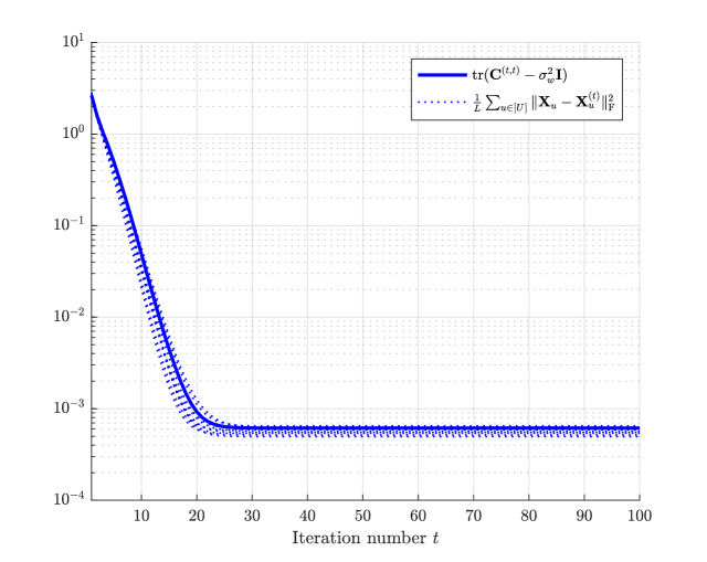
Figure 3: The finite-dimensional AMP total normalized MSE for 10 Monte Carlo samples and its theoretical deterministic prediction for the toy model example (Fig. 2) with $N_{u}=2048$, $L=1024$, $\wp=1/2$, and UL ${\sf SNR}=10$ dB .

Next, we compare the detection performances of the heuristic distributed AMP (dAMP) algorithm presented in [34],[35] and our proposed AMP algorithm in Fig. 4. dAMP applies a conventional AMP separately for each RU, and then combines the LLRs for the message activity detection. We observe that the proposed centralized AMP approach generally outperforms dAMP and its performance gain increases with the crosstalk parameter $\wp$.

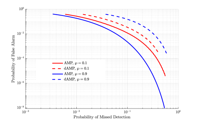
Figure 4: The performance comparison of the AMP and dAMP algorithms for the toy model example (Fig. 2) with $N_{u}=2048$, $L=1024$, and ${\sf SNR}=10$ dB.

Then, we consider a more realistic CF user-centric network. The coverage area is divided into $U=16$ location tiles with equilateral triangular shape of side $100$m, arranged in a hexagonal pattern as depicted in Fig. 5. We position $B=12$ RUs at the corners of the triangular location tiles. The message probabilities are set as $\lambda_{u}\in\{0.003,0.002\}$, repeated in a fixed alternating pattern, such that $\lambda_{1}=0.003,\lambda_{2}=0.002$, and so on. Each location-based uRA codebook ${\bf S}_{u}$ consists of $N_{u}=2048$ codewords with block length $L=1024$. We use torus-topology to calculate distances in order to approximate an infinitely large network without “border” effects. The distance-dependent pathloss (PL) function is given by

$$\text{PL}=\frac{1}{1+\left(\frac{d}{d_{0}}\right)^{\gamma}}\;,$$ (78)

with pathloss exponent $\gamma=3.67$, and 3dB cutoff distance $d_{0}=13.57\text{m}$ (this is the distance at which the received signal power from a given RU is attenuated by 3dB due to the pathloss). In order to set the UL transmit power (i.e., the parameter ${\sf SNR}$), we consider the pathloss between a location and its nearest RU. Letting $\varsigma$ denote such minimum distance and $\text{PL}_{\varsigma}=1/(1+\left(\frac{\varsigma}{d_{0}}\right)^{\gamma})$ the corresponding pathloss, we set the received SNR (at any nearest RU antenna) to be some reasonable value ${\sf SNR}_{\rm rx}$ and, as a consequence, we let ${\sf SNR}={\sf SNR}_{\rm rx}/\text{PL}_{\varsigma}$.

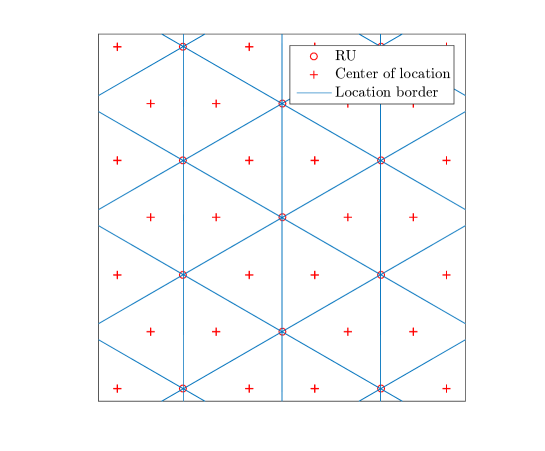
Figure 5: Hexagonal network topology with equilateral triangle tiles. The crosses denote the user locations and the circles denote the RUs.

For the system described above, we illustrate the theory-simulation consistency for the total normalized MSE of the AMP iterations, i.e. (77), in Fig. 6 for $M=2$ and ${\sf SNR}_{\rm rx}=10$dB (again, we show 10 independently generated trajectories of the finite-dimensional system and the deterministic trajectory predicted by the SE). For the same system parameters, Fig. 7 shows the theoretical predictions and the finite dimensional simulation of the misdetection and false-alarm probabilities. The theoretical prediction is obtained using the Gauss-Chebyshev Laplace inversion method reviewed in Appendix J. For each location $u$ the detection threshold in the Neyman-Pearson test (38) is varied in order to obtain the tradeoff curve. Fig. 7 shows the average tradeoff curve over all locations. In particular, the red dot corresponds to the point at which, for each location $u$, the threshold is set such that $\tilde{\rm P}^{\rm md}_{u}=\tilde{\rm P}^{\rm fa}_{u}$. All subsequent results shall be given for this choice, i.e., the system operates such that in each location the false-alarm and the misdetection probabilities are balanced.

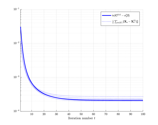
Figure 6: The total normalized MSE of the AMP iterations (8) for 10 Monte Carlo samples and its theoretical prediction for the cell free network of Fig. 5) with $N_{u}=2048$, $L=1024$, $M=2$, and ${\sf SNR}_{\rm rx}=10$ dB.

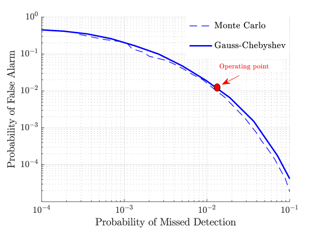
Figure 7: Average operational tradeoff curve of the message detector for the CF network of Fig. 5 with $N_{u}=2048$, $L=1024$, $M=2$, and ${\sf SNR}_{\rm rx}=10$ dB.

Next we consider the channel estimation error for the messages in ${\cal A}_{\rm d}$ (genuinely active messages, detected as active) for the system described above, operating at the point $\tilde{\rm P}^{\rm md}_{u}=\tilde{\rm P}^{\rm fa}_{u}$ as said before. With reference to Theorem 3 and (53), we can express the asymptotic total channel estimation error calculated by summing the errors (normalized by the total number of RU antennas) over all locations. This comparison is shown in Fig. 8. In general, we observe that when operating with sufficiently low ${\rm P}^{\rm md}_{u}$ and ${\rm P}^{\rm fa}_{u}$ (in our case, $\approx 10^{-2}$, as seen from Fig. 7), the channel estimation performance of the joint AMP-based message detection and channel estimation is very close to the performance of the genie-aided MMSE estimation and no further reprocessing is needed.

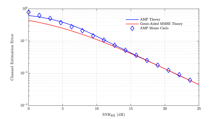
Figure 8: Channel estimation error for the genie-aided MMSE, the asymptotic theory (AMP), and the finite dimensional AMP simulation (Monte Carlo), where the latter is calculated for the set of efectively detected active messages ${\cal A}_{\rm d}$, averaged over 100 Monte Carlo runs.

Following the scheme described in Section 5, the RACH slot is followed by a DL transmission (referred to as ACK slot) to the users corresponding to the detected uRA messages $\widehat{{\cal A}}$. In this example, we consider that each location is served by the $Q=3$ nearest RUs using MRT based on the estimated channel vectors. Fig. 9 shows the CDF of the per-user rate (computed via the UatF achievable lower bound (72) ) and, for comparison, the corresponding CDF of the genie-aided UatF bound given in (76). Since these rate expressions depend only on the location index $u$ and not on the message index $n$, these CDFs have a “staircase” shape with jumps corresponding to the rates at different locations $u$. For example, if all locations have distinct rate values, we have $U$ jumps and the $u$-th jump has amplitude (assuming very small ${\rm P}^{\rm md}_{u}$ and ${\rm P}^{\rm fa}_{u}$, i.e., ${\cal A}=\widehat{{\cal A}}$) equal to $\lambda_{u}N_{u}/(\sum_{u^{\prime}}\lambda_{u^{\prime}}N_{u^{\prime}})$, i.e., the relative fraction of active users in location $u$.

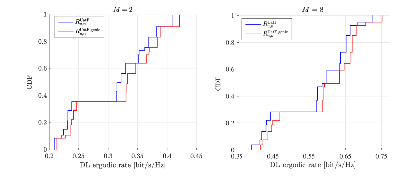
Figure 9: Achievable per-user ergodic rate CDF of the DL ACK message under MRT precoding for the CF network of Fig. 5 with $N_{u}=2048$, $L=1024$, and ${\sf SNR}_{\rm rx}=10$ dB.

Fig. 9 shows that when the system is sized to operate with low message error probability and low channel estimation error, as in this case, the achievable per-user rate is very close to the ideal case (perfect uRA message detection and CSI). We also illustrate the effect of the number of antennas per uRA on the user rates for $M=\{2,8\}$. Indeed, the median user rate for $M=2$ is $\approx 0.32$ bit/symbol, while for $M=8$ it increases to $\approx 0.6$ bit/symbol.

7 Conclusion

We considered the problem of unsourced random access (uRA) in cell-free wireless networks. The model is an extension of what already considered in several works for the case of uRA with a massive MIMO receiver. The difference is that, in the cell-free case, the total number of antennas $BM$ is partitioned in $B$ groups of $M$ antennas each, and these are allocated to geographically separated RUs. While this may seem a minor modification, the problem is significantly more complicated by the fact that the statistics of the channel vectors describing the propagation between users and RUs dependents on the user (transmitter) location, via the set of distance-dependent large-scale fading coefficients between the user and the RUs. In the uRA setting, users can transmit any codeword from a common codebook. It is therefore not possible to associate in a fixed manner a given access codeword to a given set of large-scale propagation coefficients (unlike the problem of activity detection with known user locations and fixed association between activity “signature” sequences and users). We circumvent this problem by proposing a partitioned access codebook associating sub-codebooks to “locations”, such that users in a given location select codewords from the corresponding codebook. For this system, we propose a centralized AMP algorithm for joint uRA message detection and CSI estimation. The rigorous analysis of this AMP scheme is novel and does not reduces immediately to a known case for which the asymptotic SE analysis and concentration result has been rigorously proved. In fact, our results yield immediately other known concentration results the classical AMP and the MMV-AMP, obtained as special cases of our general setting for $U=F=1$ and for $U=1,F>1$, respectively. In addition, we also show the consistency of the replica symmetry (non-rigorous) results with the rigorous SE analysis.

Based on our analysis, a rigorous (asymptotic) characterization of the statistics at the output of the AMP detection/estimation scheme are given. Using these statistics, we can provide very accurate and almost closed-form expressions for the false-alarm and misdetection probabilities of the uRA messages. Also, using the asymptotic statistics, simple and almost closed-form expressions for the achievable user rate in a subsequent transmission phase are obtained. For simplicity, we focused here on the downlink transmission based on MRT, which requires only per-RU local combining CSI. However, in a similar manner, expressions for other forms of combining/precoding can be obtained for both downlink and uplink transmission (in the latter case, after the RACH slot the user would append a data communication slot as in the scheme of [24]).

As an outlook to future work, it is interesting to assess the performance of networks where the users are randomly distributed and not concentrated at “location centroids” as in this work. The SE and concentration law presented here holds also for this case, where the AMP algorithm is “mismatched”, i.e., it assumes the “nominal” LSFCs at the location centroids, while the position of the uRA users is arbitrarily distributed on the whole location area. Preliminary results in this sense (which will be presented in a separate work) show that the effect of this mismatch is essentially negligible, if the locations are appropriately defined and the pathloss function is sufficiently smooth.

Another interesting extension is the case where the number of antennas per RU scales with the number of uRA messages (i.e.,, with $L$). In this case, we let the number of antennas per RU be equal to $mM$, where $M$ is fixed (constant with $L$) and $m/L=\beta$. Then, each block of $M$ antennas forms a system identical to the one presented in this paper, for which the concentration holds. However, for the sake of message detection and data transmission, the $m$ group of antennas at each RU can be “pooled” together. This yields vanishing message error probability (both false-alarm and misdetection) and non-vanishing per-user rate as $L\rightarrow\infty$. Again, these results will be presented in a follow-up paper.

Finally, we notice that the symbol synchronous frequency-flat channel model used in most existing uRA. MIMO papers (starting from [20], all related papers referenced here including the present paper), is unrealistic. Propagation goes through frequency-selective multipath channels, and transmission in the RACH slot cannot be perfectly chip-level synchronous at each RU receiver, since propagation distances are different for different users and RUs. Hence, the extension to a wideband frequency-selective asynchronous model, where the unknown channels are vectors of multipath impulse responses is called for.

We conclude by emphasizing the broader applicability of our theoretical results. They go beyond the context of wireless networks and are relevant to the general problem of “multiple measurement vector” compressed sensing involving the superposition of multiple signal sources, each with different statistical characteristics. This suggests the relevance of our results to a wider range of applications.

Appendix A Preliminaries: Concentration Inequalities with $\mathcal{L}^{p}$ norm

We introduce a notion of concentration inequalities in terms of the $\mathcal{L}^{p}$ norm and present its elementary properties which are frequently used in the following proofs.

We recall the scaling of model parameters in Assumption 2. Also, for convenience, we write $N\asymp L$ to imply that the ratio $N/L$ is fixed as $L\to\infty$. Let $\kappa_{L}$ be a deterministic and positive sequence indexed by $L$ (e.g., $\kappa_{L}=L^{-1/2}$ or $\kappa_{L}=1$). We write ${a}=\mathcal{O}(\kappa_{L})$ if for all $p\in\mbox{\bb N}$ there is a constant $C_{p}$ such that

$$\|{a}\|_{\mathcal{L}^{p}}\leq C_{p}\kappa_{L}\;.$$ (79)

In general, let ${\bf A}=\big{(}{\bf A}^{(L)}\big{)}$ be a family of random matrices indexed by $L$. Then, with some (slight) abuse of notation, we write ${\bf A}=\mathcal{O}(\kappa_{L})$ to indicate $\|{\bf A}\|_{\rm F}=\mathcal{O}(\kappa_{L})$. If $\widehat{{\bf A}}-{\bf A}=\mathcal{O}(1)$, we say that $\widehat{{\bf A}}$ is a high-dimensional equivalent of ${\bf A}$, denoted by

$$\widehat{{\bf A}}\simeq{\bf A}\;.$$ (80)

Lemma 1.

Consider the (scalar) random variables ${a}=\mathcal{O}(\kappa_{L})$ and ${b}=\mathcal{O}(\tilde{\kappa}_{L})$, where $\kappa_{L}$ and $\tilde{\kappa}_{L}$ are two positive sequences indexed by $L$. Then the following properties hold:

$${a+b} =\mathcal{O}(\max(\kappa_{L},\tilde{\kappa}_{L}))$$ (81)

$${ab} =\mathcal{O}(\kappa_{L}\tilde{\kappa}_{L})$$ (82)

$$\sqrt{a} =\mathcal{O}(\sqrt{\kappa_{L}}).$$ (83)

Proof.

The results (81) and (82) follow from the Minkowski inequality and Hölder’s inequality, (i.e. $\|{a}+{\rm b}\|_{\mathcal{L}^{p}}\leq\|{a}\|_{\mathcal{L}^{p}}+\|{\rm b}\|_{\mathcal{L}^{p}}$ and $\|{a}{\rm b}\|_{\mathcal{L}^{p}}\leq\|{a}\|_{\mathcal{L}^{2p}}\|{\rm b}\|_{\mathcal{L}^{2p}}$), respectively. The result (83) follows from $\|{a}^{1/2}\|_{\mathcal{L}^{p}}\leq\|{a}^{1/2}\|_{\mathcal{L}^{2p}}=\|{a}\|_{\mathcal{L}^{p}}^{\frac{1}{2}}$. ∎

Lemma 2.

[55, Lemma 7.8] For $N\asymp L$, define the random vector $\underline{{\bf a}}\in\mbox{\bb C}^{N}$ with $\underline{{\bf a}}\sim_{\rm i.i.d.}a$, where ${a}$ is a random variable with ${a}=\mathcal{O}(1)$. Then, we have

$$\frac{1}{N}\sum_{n\in[N]}{a}_{n}=\mathbb{E}[{a}]+\mathcal{O}(L^{-1/2})\;.$$

Lemma 3.

For $N\asymp L$, consider the random vectors $\underline{{\bf a}},\underline{{\bf b}}\in\mathbb{C}^{N}$ where $\underline{{\bf a}}\sim_{\text{i.i.d.}}a$ and $\underline{{\bf b}}\sim_{\text{i.i.d.}}b$ with ${a}=\mathcal{O}(1)$ and $b=\mathcal{O}(1)$. Then, for any $\widehat{\underline{{\bf a}}}\simeq\underline{{\bf a}}$ and $\underline{\widehat{\bf b}}\simeq\underline{{\bf b}}$, we have

$$\frac{1}{N}\widehat{\underline{{\bf a}}}^{\sf H}\underline{\widehat{\bf b}}=\mathbb{E}[a^{\star}{b}]+\mathcal{O}(L^{-1/2})\;.$$ (84)

Proof.

Let $\underline{{\mathchoice{\mbox{\boldmath$\displaystyle\delta$}}{\mbox{\boldmath$\textstyle\delta$}}{\mbox{\boldmath$\scriptstyle\delta$}}{\mbox{\boldmath$\scriptscriptstyle\delta$}}}_{a}}\stackrel{{\scriptstyle\Delta}}{{=}}\widehat{\underline{{\bf a}}}-{\underline{{\bf a}}}$ and $\underline{{\mathchoice{\mbox{\boldmath$\displaystyle\delta$}}{\mbox{\boldmath$\textstyle\delta$}}{\mbox{\boldmath$\scriptstyle\delta$}}{\mbox{\boldmath$\scriptscriptstyle\delta$}}}_{b}}\stackrel{{\scriptstyle\Delta}}{{=}}\widehat{\underline{{\bf b}}}-{\underline{{\bf b}}}$ with noting that e.g. $\underline{{\mathchoice{\mbox{\boldmath$\displaystyle\delta$}}{\mbox{\boldmath$\textstyle\delta$}}{\mbox{\boldmath$\scriptstyle\delta$}}{\mbox{\boldmath$\scriptscriptstyle\delta$}}}_{a}}=\mathcal{O}(1)$. From Lemma 2 we have $\underline{{\bf a}}=\mathcal{O}(\sqrt{L})$ and $\underline{{\bf b}}=\mathcal{O}(\sqrt{L})$. Hence, we get from the arithmetic rules (82) and (81) that

$$\underline{\widehat{\bf a}}^{\sf H}\underline{\widehat{\bf b}}-{\underline{{\bf a}}}^{\sf H}\underline{{\bf b}}=\underline{{\bf a}}^{\sf H}\underline{{\mathchoice{\mbox{\boldmath$\displaystyle\delta$}}{\mbox{\boldmath$\textstyle\delta$}}{\mbox{\boldmath$\scriptstyle\delta$}}{\mbox{\boldmath$\scriptscriptstyle\delta$}}}_{b}}+\underline{{\bf b}}^{\sf H}\underline{{\mathchoice{\mbox{\boldmath$\displaystyle\delta$}}{\mbox{\boldmath$\textstyle\delta$}}{\mbox{\boldmath$\scriptstyle\delta$}}{\mbox{\boldmath$\scriptscriptstyle\delta$}}}_{a}}+\underline{{\mathchoice{\mbox{\boldmath$\displaystyle\delta$}}{\mbox{\boldmath$\textstyle\delta$}}{\mbox{\boldmath$\scriptstyle\delta$}}{\mbox{\boldmath$\scriptscriptstyle\delta$}}}_{a}}^{\sf H}\underline{{\mathchoice{\mbox{\boldmath$\displaystyle\delta$}}{\mbox{\boldmath$\textstyle\delta$}}{\mbox{\boldmath$\scriptstyle\delta$}}{\mbox{\boldmath$\scriptscriptstyle\delta$}}}_{b}}=\mathcal{O}(\sqrt{L})\;.$$ (85)

Second, from the rule (82) we have $a^{\star}b=\mathcal{O}(1)$. Thus, from Lemma 2 we have the concentration $\frac{1}{N}{\underline{{\bf a}}}^{\sf H}\underline{{\bf b}}=\mathbb{E}[a^{\star}{b}]+\mathcal{O}(L^{-1/2})$. This completes the proof. ∎

Appendix B Proof of Theorem 1

In this section, we provide a nearly self-contained proof of Theorem 1. Auxiliary lemmas are proved in Appendix G in order to maintain the flow of exposition. The proof of Theorem 1 relies on the idea of the "Householder dice" representation of AMP dynamics introduced in [56]. Such a representation can be seen as an intermediate step in the commonly used "conditioning" AMP proof technique [57]. Namely, it clarifies how to represent the original AMP dynamics - that are coupled by a random matrix (${\bf S}_{u}$, in our case) - as equivalent dynamics without a random matrix (i.e., ${\bf S}_{u}$-free). This step has no approximation and requires no assumption other than the underlying random matrix assumption (i.e., ${\bf S}_{u}\sim\mathcal{CN}({\mathchoice{\mbox{\boldmath$\displaystyle 0$}}{\mbox{\boldmath$\textstyle 0$}}{\mbox{\boldmath$\scriptstyle 0$}}{\mbox{\boldmath$\scriptscriptstyle 0$}}},{\bf I}_{N_{u}}/L)$). We also refer the reader to [58] where a similar AMP proof strategy is used.

At a high level, we have two main steps in the proof. In the first step (Section B.1), we use the block Gram-Schmidt process to express the dynamics of AMP (8) in terms of an equivalent ${\bf S}_{u}$-free dynamics, called the "Householder dice representation". In the second step (Section B.2), we use the properties of the notion of $\mathcal{L}^{p}$ concentration given in Appendix A to establish the high-dimensional equivalence of the Householder dice representation, and thereby it will give us the high-dimensional equivalent of the original AMP dynamics (8).

For convenience, we will use the following notation for matrices throughout the proof: Consider matrices ${\bf A}$ and ${\bf B}$, both with the same number of rows, denoted by $N$. Then, we define

$$\langle{\bf A},{\bf B}\rangle\stackrel{{\scriptstyle\Delta}}{{=}}\frac{1}{N}{\bf A}^{{\sf H}}{\bf B}$$ (86)

whenever the dependency on $N$ is clear from the context.

B.1 Step-1: The Householder dice equivalent

We will use an adaptive representation of the Gaussian random matrices (i.e., ${\bf S}_{u}$ in the context) by using the following result (see also [56, Eq. (11)]).

Lemma 4.

Let the random matrices ${\bf V}\in\mathbb{C}^{L\times F}$, ${\bf U}\in\mathbb{C}^{N\times F}$ and $\tilde{{\bf S}}\in\mathbb{C}^{L\times N}$ be mutually independent. Let ${\bf P}_{\bf V}^{\perp}\stackrel{{\scriptstyle\Delta}}{{=}}{\bf I}-\frac{1}{L}{\bf V}{\bf V}^{\sf H}$ be a projection matrix, ${\bf U}\sim_{\text{i.i.d.}}\mathcal{CN}({\mathchoice{\mbox{\boldmath$\displaystyle 0$}}{\mbox{\boldmath$\textstyle 0$}}{\mbox{\boldmath$\scriptstyle 0$}}{\mbox{\boldmath$\scriptscriptstyle 0$}}},{\bf I}_{F})$ and $\tilde{\bf S}\sim_{\text{i.i.d.}}\mathcal{CN}({\mathchoice{\mbox{\boldmath$\displaystyle 0$}}{\mbox{\boldmath$\textstyle 0$}}{\mbox{\boldmath$\scriptstyle 0$}}{\mbox{\boldmath$\scriptscriptstyle 0$}}},{\bf I}_{N}/L)$. Let

$${\bf S}=\frac{{\bf V}{\bf U}^{\sf H}}{L}+{\bf P}_{\bf V}^{\perp}\tilde{\bf S}\;.$$ (87)

Then, ${\bf S}\sim\tilde{\bf S}$ and ${\bf S}$ is (statistically) independent of ${\bf V}$.

Proof.

Let ${\rm vec}({\bf S})$ denote the column vector obtained by stacking the column vectors of ${\bf S}$ below one another, i.e. ${\rm vec}({\bf S})=[\underline{{\bf s}}_{1}^{\top},\underline{{\bf s}}_{2}^{\top},\cdots\underline{{\bf s}}_{N}]^{\top}$. Then, conditioned on ${\bf V}$, it is easy to verify that ${\rm vec}({{\bf S}})$ is a complex Gaussian vector with zero mean and covariance

$${\bf I}_{N}\otimes\left(\frac{1}{L^{2}}{\bf V}{\bf V}^{\sf H}+\frac{1}{L}({\bf P}_{\bf V}^{\perp})^{2}\right) ={\bf I}_{N}\otimes\left(\frac{1}{L^{2}}{\bf V}{\bf V}^{\sf H}+\frac{1}{L}{\bf P}_{\bf V}^{\perp}\right)$$ (88)

$$={\bf I}_{N}\otimes\frac{1}{L}{\bf I}_{L}\;.$$ (89)

Thereby, conditioned on ${\bf V}$, we have ${\bf S}\sim_{\text{i.i.d.}}\mathcal{CN}({\mathchoice{\mbox{\boldmath$\displaystyle 0$}}{\mbox{\boldmath$\textstyle 0$}}{\mbox{\boldmath$\scriptstyle 0$}}{\mbox{\boldmath$\scriptscriptstyle 0$}}},{\bf I}_{N}/L)$. Furthermore, since the conditional distribution of ${\bf S}$ is invariant from ${\bf V}$, ${\bf S}$ and ${\bf V}$ are independent. ∎

Note that we can also consider the conjugate representation of Lemma 4 as

$${\bf S}^{\sf H}=\frac{{\bf U}{\bf V}^{\sf H}}{L}+\tilde{\bf S}^{\sf H}{\bf P}_{\bf V}^{\perp}$$ (90)

For example, let us consider a matrix ${\bf Z}\in\mbox{\bb C}^{L\times F,}$ with $\text{span}({\bf Z})=\text{span}({\bf V})$. So that ${\bf P}_{{\bf V}}^{\perp}{\bf Z}={\mathchoice{\mbox{\boldmath$\displaystyle 0$}}{\mbox{\boldmath$\textstyle 0$}}{\mbox{\boldmath$\scriptstyle 0$}}{\mbox{\boldmath$\scriptscriptstyle 0$}}}$. Hence, we have the representation of the product ${\bf S}^{\sf H}{\bf Z}$

$${\bf S}^{\sf H}{\bf Z} ={\bf U}\langle{\bf V},{\bf Z}\rangle$$ (91)

which involves solely the lower-dimensional random element ${\bf U}\sim_{\text{i.i.d.}}\mathcal{CN}({\mathchoice{\mbox{\boldmath$\displaystyle 0$}}{\mbox{\boldmath$\textstyle 0$}}{\mbox{\boldmath$\scriptstyle 0$}}{\mbox{\boldmath$\scriptscriptstyle 0$}}},{\bf I}_{F})$.

To extend this idea to e.g. the dynamics ${\bf S}_{u}^{\sf H}{\bf Z}^{(t)}$ (and similarly to the dynamics ${\bf S}_{u}{\mathchoice{\mbox{\boldmath$\displaystyle{\bf X}$}}{\mbox{\boldmath$\textstyle{\bf X}$}}{\mbox{\boldmath$\scriptstyle{\bf X}$}}{\mbox{\boldmath$\scriptscriptstyle{\bf X}$}}}_{u}^{(t)}$), we will employ the block Gram-Schmidt process to construct a set of ”orthogonal” matrices, denoted as ${\bf V}^{(1:t)}\equiv\{{\bf V}^{(1)},{\bf V}^{(2)},\ldots,{\bf V}^{(t)}\}$ such that $\text{span}({\bf V}^{(1:t)})=\text{span}({\bf Z}^{(1:t)})$. We then recursively apply Lemma 4 to obtain an ${\bf S}_{u}$-free equivalent of the dynamics ${\bf S}_{u}^{\sf H}{\bf Z}^{(t)}$.

We first introduce the block Gram-Schmidt notation: Let ${\bf V}^{(1:t-1)}=\{{\bf V}^{(1)},{\bf V}^{(2)},\ldots,{\bf V}^{(t-1)}\}$ be a collection of matrices in $\mbox{\bb C}^{N\times F}$ with $\langle{\bf V}^{(i)},{\bf V}^{(j)}\rangle=\mathcal{\delta}_{ij}{\bf I}_{F}$ for all $i,j$. Then, for any matrix ${\bf B}\in\mbox{\bb C}^{N\times F}$, by using the block Gram-Schmidt (orthogonalization) process, we can always construct the new (semi-unitary) matrix

$${\bf V}^{(t)}\overset{\text{def}}{=}\mathcal{GS}({\bf B}\mid{\bf V}^{(1:t-1)})$$

such that $\langle{\bf V}^{(t)},{\bf V}^{(s)}\rangle=\delta_{st}{\bf I}_{F}$ and we have the block ”Gram-Schmidt decomposition"

$${\bf B}=\sum_{1\leq s\leq t}{\bf V}^{(s)}\langle{\bf V}^{(s)},{\bf B}\rangle\;.$$ (92)

We refer to Appendix K for the explicit definition of the block Gram-Schmidt notation.

B.1.1 Iteration Step $t=1$

We begin with deriving the Householder dice representation of the AMP dynamics (8) for the iteration step $t=1$. For convenience, we set ${\bf X}_{u}^{(0)}\equiv{\bf X}_{u}$ (for all $u\in[U]$). Let

$${\bf V}_{u}^{(0)} \stackrel{{\scriptstyle\Delta}}{{=}}\mathcal{GS}({\bf X}_{u}^{(0)}\mid\emptyset).$$ (93)

Note that we have the block Gram-Schmidt (i.e. QR) decomposition

$${\bf X}_{u}^{(0)}={\bf V}_{u}^{(0)}\langle{\bf V}_{u}^{(0)},{\bf X}_{u}^{(0)}\rangle$$ (94)

Also, we have the projection matrix to the orthogonal complement of $\text{span}({\bf X}_{u}^{(0)})$ as

$${\bf P}_{{\bf X}_{u}^{(0)}}^{\perp}={\bf I}-\frac{1}{N_{u}}{\bf V}_{u}^{(0)}({\bf V}_{u}^{(0)})^{\sf H}\;.$$ (95)

Second, we introduce the matrix

$${\bf G}_{u}^{(0)}\stackrel{{\scriptstyle\Delta}}{{=}}\frac{1}{\sqrt{\alpha_{u}}}{\bf S}_{u}{\bf V}_{u}^{(0)}\;$$ (96)

Notice that conditioned on ${\bf V}_{u}^{(0)}$

$${\bf G}_{u}^{(0)}\sim_{\text{i.i.d.}}\mathcal{CN}({\mathchoice{\mbox{\boldmath$\displaystyle 0$}}{\mbox{\boldmath$\textstyle 0$}}{\mbox{\boldmath$\scriptstyle 0$}}{\mbox{\boldmath$\scriptscriptstyle 0$}}};{\bf I}_{F})\;.$$ (97)

Thus, ${\bf G}_{u}^{(0)}$ is independent of ${\bf V}_{u}^{(0)}$. Then, we use Lemma 4 (specifically, the conjugate representation in (90)) to represent ${\bf S}_{u}$ as

$${\bf S}_{u}={\sqrt{\alpha_{u}}}\frac{{\bf G}_{u}^{(0)}({\bf V}_{u}^{(0)})^{\sf H}}{N_{u}}+{\bf S}_{u}^{(0,0)}{\bf P}_{{\bf X}_{u}^{(0)}}^{\perp}$$ (98)

where ${\bf S}_{u}^{(0,0)}\sim{\bf S}_{u}$ is an arbitrary (independent of everything else constructed before) random element. Moving forward, let

$${\bf V}_{u}^{(1)}=\mathcal{GS}({\bf X}_{u}^{(1)}\mid{\bf V}_{u}^{(0)})\;.$$ (99)

Then, we use Lemma 4 to represent ${\bf S}_{u}^{(0,0)}$ in (98) as

$${\bf S}_{u}^{(0,0)}={\sqrt{\alpha_{u}}}\frac{{\bf G}_{u}^{(1)}({\bf V}_{u}^{(1)})^{\sf H}}{N_{u}}+{\bf S}_{u}^{(0,1)}{\bf P}_{{\bf V}_{u}^{(1)}}^{\perp}$$ (100)

where we introduce the new arbitrary random matrices ${\bf G}_{u}^{(1)}\sim{\bf G}_{u}^{(0)}$ and ${\bf S}_{u}^{(0,1)}\sim{\bf S}_{u}$. Then, plugging the expression (100) into (98) yields the representation

$${\bf S}_{u}={\sqrt{\alpha_{u}}}\frac{{\bf G}_{u}^{(0)}({\bf V}_{u}^{(0)})^{\sf H}}{N_{u}}+{\sqrt{\alpha_{u}}}\frac{{\bf G}_{u}^{(1)}({\bf V}_{u}^{(1)})^{\sf H}}{N_{u}}+{\bf S}_{u}^{(0,1)}{\bf P}_{{\bf X}_{u}^{(0:1)}}^{\perp}\;,$$ (101)

Here, ${\bf P}_{{\bf X}_{u}^{(0:1)}}^{\perp}$ is the projection matrix to the orthogonal complement of the span of ${\bf X}_{u}^{(0:1)}$:

$${\bf P}_{{\bf X}_{u}^{(0:1)}}^{\perp}={\bf I}-\frac{1}{N}_{u}\sum_{0\leq s^{\prime}\leq 1}{\bf V}_{u}^{(s^{\prime})}({\bf V}_{u}^{(s^{\prime})})^{\sf H}\;.$$

Note that ${\bf P}_{{\bf X}_{u}^{(0:1)}}^{\perp}{\bf X}_{u}^{(1)}={\mathchoice{\mbox{\boldmath$\displaystyle 0$}}{\mbox{\boldmath$\textstyle 0$}}{\mbox{\boldmath$\scriptstyle 0$}}{\mbox{\boldmath$\scriptscriptstyle 0$}}}$. Then, from the (101) we have

$${\mathchoice{\mbox{\boldmath$\displaystyle\Gamma$}}{\mbox{\boldmath$\textstyle\Gamma$}}{\mbox{\boldmath$\scriptstyle\Gamma$}}{\mbox{\boldmath$\scriptscriptstyle\Gamma$}}}_{u}^{(1)} ={\bf S}_{u}{\bf X}_{u}^{(1)}$$ (102)

$$={\sqrt{\alpha_{u}}}{\bf G}_{u}^{(0)}\langle{\bf V}_{u}^{(0)},{\bf X}_{u}^{(1)}\rangle+{\sqrt{\alpha_{u}}}{\bf G}_{u}^{(1)}\langle{\bf V}_{u}^{(1)},{\bf X}_{u}^{(1)}\rangle\;.$$ (103)

To derive the ${\bf S}_{u}$-free representation of ${\mathchoice{\mbox{\boldmath$\displaystyle{\bf R}$}}{\mbox{\boldmath$\textstyle{\bf R}$}}{\mbox{\boldmath$\scriptstyle{\bf R}$}}{\mbox{\boldmath$\scriptscriptstyle{\bf R}$}}}_{u}^{(1)}$ we first construct the $L\times F$ unitary matrix

$${\bf V}^{(1)}=\mathcal{GS}({\bf Z}^{(1)}\mid\emptyset)$$

and use Lemma 4 to represent ${\bf S}_{u}^{(0,1)}$ in (101)  as

$${\bf S}_{u}^{(0,1)}=\frac{{\bf V}^{(1)}({\bf U}_{u}^{(1)})^{\sf H}}{L}+{\bf P}_{{\bf Z}^{(1)}}^{\perp}{\bf S}_{u}^{(1,1)}$$ (104)

where we have introduced the new arbitrary random matrices ${\bf S}_{u}^{(1,1)}\sim{\bf S}_{u}$ and ${{\bf U}}_{u}^{(1)}\in\mbox{\bb C}^{N_{u}\times F}$ with ${{\bf U}}_{u}^{(1)}\sim_{\text{i.i.d.}}\mathcal{CN}({\mathchoice{\mbox{\boldmath$\displaystyle 0$}}{\mbox{\boldmath$\textstyle 0$}}{\mbox{\boldmath$\scriptstyle 0$}}{\mbox{\boldmath$\scriptscriptstyle 0$}}};{\bf I}_{F})$. Hence, (101) reads as

$${\bf S}_{u} ={\sqrt{\alpha_{u}}}\frac{{\bf G}_{u}^{(0)}({\bf V}_{u}^{(0)})^{\sf H}}{N_{u}}+{\sqrt{\alpha_{u}}}\frac{{\bf G}_{u}^{(1)}({\bf V}_{u}^{(1)})^{\sf H}}{N_{u}}+\frac{{\bf V}^{(1)}(\widehat{\bf U}_{u}^{(1)})^{\sf H}}{L}+{\bf P}_{{\bf Z}^{(1)}}^{\perp}{\bf S}_{u}^{(1,1)}{\bf P}_{{\bf X}_{u}^{(0:1)}}^{\perp}$$ (105)

where for short we define

$$\widehat{{\bf U}}_{u}^{(1)}\stackrel{{\scriptstyle\Delta}}{{=}}{\bf P}_{{\bf X}_{u}^{(0:1)}}^{\perp}{{\bf U}}_{u}^{(1)}\;.$$

Note that ${\bf P}_{{\bf Z}^{(1)}}^{\perp}{\bf Z}^{(1)}={\mathchoice{\mbox{\boldmath$\displaystyle 0$}}{\mbox{\boldmath$\textstyle 0$}}{\mbox{\boldmath$\scriptstyle 0$}}{\mbox{\boldmath$\scriptscriptstyle 0$}}}$. Then, from (105) we have

$${\bf R}_{u}^{(1)} ={\bf S}_{u}^{\sf H}{\bf Z}^{(1)}+{\bf X}_{u}^{(1)}$$ (106)

$$=\frac{1}{\sqrt{\alpha_{u}}}{\bf V}_{u}^{(0)}\langle{\bf G}_{u}^{(0)},{\bf Z}^{(1)}\rangle+\frac{1}{\sqrt{\alpha_{u}}}{\bf V}_{u}^{(1)}\langle{\bf G}_{u}^{(1)},{\bf Z}^{(1)}\rangle+\widehat{\bf U}_{u}^{(1)}\langle{\bf V}^{(1)},{\bf Z}^{(1)}\rangle+{\bf X}_{u}^{(1)}$$ (107)

$$={\bf V}_{u}^{(0)}(\frac{1}{\sqrt{\alpha_{u}}}\langle{\bf G}_{u}^{(0)},{\bf Z}^{(1)}\rangle+\langle{\bf V}_{u}^{(0)},{\bf X}_{u}^{(1)}\rangle)+\widehat{\bf U}_{u}^{(1)}\langle{\bf V}^{(1)},{\bf Z}^{(1)}\rangle$$

$$+{\bf V}_{u}^{(1)}(\frac{1}{\sqrt{\alpha_{u}}}\langle{\bf G}_{u}^{(1)},{\bf Z}^{(1)}\rangle+\langle{\bf V}_{u}^{(1)},{\bf X}_{u}^{(1)}\rangle)\;.$$ (108)

In step (108) we use the block Gram-Schmidt decomposition

$${\bf X}_{u}^{(1)}=\sum_{s=0}^{1}{\bf V}_{u}^{(s)}\langle{\bf V}_{u}^{(s)},{\bf X}_{u}^{(1)}\rangle\;.$$ (109)

This completes the Householder dice representation of the AMP dynamics of (8) for $t=1$.

B.1.2 Iteration Step $t=2$

Moving on to the second iteration step, we fix $t=2$ but mimic the notations in a manner that the arguments can be recalled for any $t>1$. We construct the matrices (for each $u\in[U]$)

$${\bf V}_{u}^{(t)} =\mathcal{GS}({\bf X}_{u}^{(t)}\mid{\mathchoice{\mbox{\boldmath$\displaystyle{\bf V}$}}{\mbox{\boldmath$\textstyle{\bf V}$}}{\mbox{\boldmath$\scriptstyle{\bf V}$}}{\mbox{\boldmath$\scriptscriptstyle{\bf V}$}}}_{u}^{(0:t-1)}).$$ (110)

Then, using Lemma 4, we represent ${\bf S}_{u}^{(t-1,t-1)}$ (i.e. ${\bf S}_{u}^{(1,1)}$ in (105)) as

$${\bf S}_{u}^{(t-1,t-1)}={\sqrt{\alpha_{u}}}\frac{{\bf G}_{u}^{(t)}({\bf V}_{u}^{(t)})^{\sf H}}{N_{u}}+{\bf S}_{u}^{(t-1,t)}{\bf P}_{{\bf V}_{u}^{(t)}}^{\perp}\;,$$ (111)

where we introduce the new arbitary random matrices ${\bf S}_{u}^{(t-1,t)}\sim{\bf S}_{u}$ and ${\bf G}_{u}^{(t)}\sim{\bf G}_{u}^{(0)}$. Then, (105) reads as

$${\bf S}_{u} ={\sqrt{\alpha_{u}}}\frac{{\bf G}_{u}^{(0)}({\bf V}_{u}^{(0)})^{\sf H}}{N_{u}}+{\sqrt{\alpha_{u}}}\sum_{s=1}^{t}\frac{\widehat{\bf G}_{u}^{(s)}({\bf V}_{u}^{(s)})^{\sf H}}{N_{u}}+\sum_{s=1}^{t-1}\frac{{\bf V}^{(s)}(\widehat{\bf U}_{u}^{(s)})^{\sf H}}{L}+{\bf P}_{{\bf Z}^{(1:t-1)}}^{\perp}{\bf S}_{u}^{(t-1,t)}{\bf P}_{{\bf X}_{u}^{(0:t)}}^{\perp}\;\;.$$ (112)

Here the matrices ${\bf P}_{{\bf X}_{u}^{(0:t)}}^{\perp}$ and ${\bf P}_{{\bf Z}^{(1:t-1)}}^{\perp}$ denote the projections onto the orthogonal complement of the subspaces spanned by ${\bf X}_{u}^{(0:t)}$ and ${\bf Z}^{(1:t-1)}$, respectively. For example,

$${\bf P}_{{\bf Z}^{(1:t-1)}}^{\perp}={\bf I}-\frac{1}{L}\sum_{s=1}^{t-1}{\bf V}^{(s)}({\bf V}^{(s)})^{\sf H}\;.$$

Also, for convenience, we have defined

$$\widehat{{\bf G}}_{u}^{(t)}\stackrel{{\scriptstyle\Delta}}{{=}}{\bf P}_{{\bf Z}^{(1:t-1)}}^{\perp}{{\bf G}}_{u}^{(t)}\;.$$

Then, by using the representation (112) we obtain

$${\mathchoice{\mbox{\boldmath$\displaystyle\Gamma$}}{\mbox{\boldmath$\textstyle\Gamma$}}{\mbox{\boldmath$\scriptstyle\Gamma$}}{\mbox{\boldmath$\scriptscriptstyle\Gamma$}}}_{u}^{(t)} ={\sqrt{\alpha_{u}}}{\bf G}_{u}^{(0)}\langle{\bf V}_{u}^{(0)},{\bf X}_{u}^{(t)}\rangle+{\sqrt{\alpha_{u}}}\sum_{s=1}^{t}\widehat{\bf G}_{u}^{(s)}\langle{\bf V}_{u}^{(s)},{\bf X}_{u}^{(t)}\rangle$$

$$+{\alpha_{u}}\sum_{s=1}^{t-1}{\bf V}^{(s)}\langle\widehat{\bf U}_{u}^{(s)},{\bf X}_{u}^{(t)}\rangle-{\alpha_{u}}{\bf Z}^{(t-1)}{\bf Q}_{u}^{(t)}$$ (113)

$$={\sqrt{\alpha_{u}}}{\bf G}_{u}^{(0)}\langle{\bf V}_{u}^{(0)},{\bf X}_{u}^{(t)}\rangle+{\sqrt{\alpha_{u}}}\sum_{s=1}^{t}\widehat{\bf G}_{u}^{(s)}\langle{\bf V}_{u}^{(s)},{\bf X}_{u}^{(t)}\rangle$$

$$+\frac{1}{\alpha_{u}}\sum_{s=1}^{t-1}{\bf V}^{(s)}\left(\langle\widehat{\bf U}_{u}^{(s)},{\bf X}_{u}^{(t)}\rangle-\langle{\bf V}^{(s)},{\bf Z}^{(t-1)}\rangle{\bf Q}_{u}^{(t)}\right)$$ (114)

Here, the latter step uses the block Gram-Schmidt decomposition

$${\bf Z}^{(t-1)}=\sum_{s=1}^{t-1}{\bf V}^{(s)}\langle{\bf V}^{(s)},{\bf Z}^{(t-1)}\rangle\;.$$ (115)

We now construct ${\bf V}^{(t)}=\mathcal{GS}({\bf Z}^{(t)}\mid{\bf V}^{(1:t-1)})$ and

$${\bf S}_{u}^{(t-1,t)}=\frac{{\bf V}^{(t)}({\bf U}_{u}^{(t)})^{\sf H}}{L}+{\bf P}_{{\bf Z}^{(t)}}^{\perp}{\bf S}_{u}^{(t,t)}\;$$ (116)

with the auxiliary random matrices ${\bf S}_{u}^{(t,t)}\sim{\bf S}_{u}$ and ${{\bf U}}_{u}^{(t)}\in\mbox{\bb C}^{N_{u}\times F}$ with ${{\bf U}}_{u}^{(t)}\sim_{\text{i.i.d.}}\mathcal{CN}({\mathchoice{\mbox{\boldmath$\displaystyle 0$}}{\mbox{\boldmath$\textstyle 0$}}{\mbox{\boldmath$\scriptstyle 0$}}{\mbox{\boldmath$\scriptscriptstyle 0$}}};{\bf I})$. Plugging this results in (112) leads to

$${\bf S}_{u}={\sqrt{\alpha_{u}}}\frac{{\bf G}_{u}^{(0)}({\bf V}_{u}^{(0)})^{\sf H}}{N_{u}}+{\sqrt{\alpha_{u}}}\sum_{s=1}^{t}\frac{\widehat{\bf G}_{u}^{(s)}({\bf V}_{u}^{(s)})^{\sf H}}{N_{u}}+\sum_{s=1}^{t}\frac{{\bf V}^{(s)}(\widehat{\bf U}_{u}^{(s)})^{\sf H}}{L}+{\bf P}_{{\bf V}^{(1:t)}}^{\perp}{\bf S}_{u}^{(t,t)}{\bf P}_{{\bf V}_{u}^{(0:t)}}^{\perp}\;.$$ (117)

where we have defined

$$\widehat{{\bf U}}_{u}^{(t)}\stackrel{{\scriptstyle\Delta}}{{=}}{\bf P}_{{\bf X}^{(0:t)}}^{\perp}{{\bf U}}_{u}^{(t)}\;.$$

Using this construction we get

$${\bf R}_{u}^{(t)} =\frac{1}{\sqrt{\alpha_{u}}}{\bf V}_{u}^{(0)}\langle{\bf G}_{u}^{(0)},{\bf Z}^{(t)}\rangle+\frac{1}{\sqrt{\alpha_{u}}}\sum_{s=1}^{t}{\bf V}_{u}^{(s)}\langle\widehat{\bf G}_{u}^{(s)},{\bf Z}^{(t)}\rangle+\sum_{s=1}^{t}\widehat{\bf U}_{u}^{(s)}\langle{\bf V}^{(s)},{\bf Z}^{(t)}\rangle+{\bf X}_{u}^{(t)}$$ (118)

$$={\bf V}_{u}^{(0)}(\frac{1}{\sqrt{\alpha_{u}}}\langle{\bf G}_{u}^{(0)},{\bf Z}^{(t)}\rangle+\langle{\bf V}_{u}^{(0)},{\bf X}_{u}^{(t)}\rangle)+\sum_{s=1}^{t}\widehat{\bf U}_{u}^{(s)}\langle{\bf V}^{(s)},{\bf Z}^{(t)}\rangle$$ (119)

$$+\sum_{s=1}^{t}{\bf V}_{u}^{(s)}(\frac{1}{\sqrt{\alpha_{u}}}\langle\widehat{\bf G}_{u}^{(s)},{\bf Z}^{(t)}\rangle+\langle{\bf V}_{u}^{(s)},{\bf X}_{u}^{(t)}\rangle)$$ (120)

Again, as to the latter term above, we note from block Gram-Schmidt orthogonalization that

$${\bf X}_{u}^{(t)}=\sum_{s=0}^{t}{\bf V}_{u}^{(s)}\langle{\bf V}_{u}^{(s)},{\bf X}_{u}^{(t)}\rangle\;.$$ (121)

B.1.3 Iteration Steps $t>2$

Clearly, for iteration steps $t=3,4,\ldots$, we can repeat the same arguments as for the case $t=2$. Specifically, at each $t\in~{}[T]$, we utilize equations (112) and (117) to compute ${\mathchoice{\mbox{\boldmath$\displaystyle\Gamma$}}{\mbox{\boldmath$\textstyle\Gamma$}}{\mbox{\boldmath$\scriptstyle\Gamma$}}{\mbox{\boldmath$\scriptscriptstyle\Gamma$}}}_{u}^{(t)}$ and ${\bf R}_{u}^{(t)}$ in the AMP dynamics (8), respectively. By following this process, we arrive at a ${\bf S}_{u}$-free representation of the AMP dynamics (8): We commence with the identical initialization of ${\bf X}_{u}^{(1)}$ from (8) for all $u\in[U]$ and proceed for $t=1,2,\ldots,T$ as

$${\bf V}_{u}^{(t)} =\mathcal{GS}({\bf X}_{u}^{(t)}\mid{\bf V}_{u}^{(0:t-1)})$$ (122a)

$$\widehat{{\bf G}}_{u}^{(t)} ={\bf P}_{{\bf Z}^{(1:t-1)}}^{\perp}{{\bf G}}_{u}^{(t)}$$ (122b)

$${\bf O}_{u}^{(t)} =\frac{1}{\alpha_{u}}\sum_{s=1}^{t-1}{{\bf V}^{(s)}}\left(\langle{\widehat{{\bf U}}_{u}}^{(s)},{{\bf X}}_{u}^{(t)}\rangle-\langle{\bf V}^{(s)},{\bf Z}^{(t-1)}\rangle{{\bf Q}}_{u}^{(t)}\right)$$ (122c)

$${\mathchoice{\mbox{\boldmath$\displaystyle\Gamma$}}{\mbox{\boldmath$\textstyle\Gamma$}}{\mbox{\boldmath$\scriptstyle\Gamma$}}{\mbox{\boldmath$\scriptscriptstyle\Gamma$}}}^{(t)}_{u} ={\sqrt{\alpha_{u}}}{{\bf G}_{u}^{(0)}}\langle{\bf V}_{u}^{(0)},{{\bf X}}_{u}^{(t)}\rangle+{\sqrt{\alpha_{u}}}\sum_{s=1}^{t}{\widehat{{\bf G}}_{u}^{(s)}}\langle{\bf V}^{(s)}_{u},{{\bf X}}_{u}^{(t)}\rangle+{\bf O}_{u}^{(t)}$$ (122d)

$${\bf Z}^{(t)} ={\bf Y}-\sum_{1\leq u\leq U}{\mathchoice{\mbox{\boldmath$\displaystyle\Gamma$}}{\mbox{\boldmath$\textstyle\Gamma$}}{\mbox{\boldmath$\scriptstyle\Gamma$}}{\mbox{\boldmath$\scriptscriptstyle\Gamma$}}}_{u}^{(t)}$$ (122e)

$${\bf V}^{(t)} =\mathcal{GS}({\bf Z}^{(t)}\mid{\bf V}^{(1:t-1)})$$ (122f)

$$\widehat{{\bf U}}_{u}^{(t)} ={\bf P}_{{\bf X}_{u}^{(0:t)}}^{\perp}{{\bf U}}_{u}^{(t)}$$ (122g)

$$\tilde{{\bf O}}_{u}^{(t)} =\sum_{s=1}^{t}{\bf V}_{u}^{(s)}\left(\frac{1}{\sqrt{\alpha_{u}}}\langle{\widehat{{\bf G}}}_{u}^{(s)},{\bf Z}^{(t)}\rangle+\langle{\bf V}_{u}^{(s)},{{\bf X}}_{u}^{(t)}\rangle\right)$$ (122h)

$${\bf X}_{0u}^{(t)} ={\bf V}_{u}^{(0)}(\frac{1}{\sqrt{\alpha_{u}}}{\mathchoice{\mbox{\boldmath$\displaystyle\langle$}}{\mbox{\boldmath$\textstyle\langle$}}{\mbox{\boldmath$\scriptstyle\langle$}}{\mbox{\boldmath$\scriptscriptstyle\langle$}}}{\bf G}_{u}^{(0)},{\bf Z}^{(t)}\rangle+\langle{\bf V}_{u}^{(0)},{{\bf X}}_{u}^{(t)}\rangle)$$ (122i)

$${{\bf R}}_{u}^{(t)} ={\bf X}_{0u}^{(t)}+\sum_{s=1}^{t}\widehat{{\bf U}}_{u}^{(s)}\langle{\bf V}^{(s)},{\bf Z}^{(t)}\rangle+\tilde{{\bf O}}_{u}^{(t)}$$ (122j)

$${\bf X}_{u}^{(t+1)} =\eta_{u,t}({{\bf R}}_{u}^{(t)})\;.$$ (122k)

Here, by abuse of notation, we set e.g. ${\bf V}^{(1:0)}=\emptyset$. Moreover, $\{{\bf G}_{u}^{(t)}\in\mbox{\bb C}^{L\times F},{\bf U}_{u}^{(t)}\in\mbox{\bb C}^{N_{u}\times F}:(u,t)\in[U]\times[T]\}$ is the set of all mutually independent random matrices with

$${\bf G}_{u}^{(t)}\sim_{\text{i.i.d.}}\mathcal{CN}({\mathchoice{\mbox{\boldmath$\displaystyle 0$}}{\mbox{\boldmath$\textstyle 0$}}{\mbox{\boldmath$\scriptstyle 0$}}{\mbox{\boldmath$\scriptscriptstyle 0$}}};{\bf I}_{F})~{}~{}\text{and}~{}~{}{\bf U}_{u}^{(t)}\sim_{\text{i.i.d.}}\mathcal{CN}({\mathchoice{\mbox{\boldmath$\displaystyle 0$}}{\mbox{\boldmath$\textstyle 0$}}{\mbox{\boldmath$\scriptstyle 0$}}{\mbox{\boldmath$\scriptscriptstyle 0$}}};{\bf I}_{F})\;.$$

Furthermore, we use the notations ${\bf O}_{u}^{(t)}$ and $\tilde{\bf O}_{u}^{(t)}$ to associate the so-called Onsager memory cancellations. Indeed, we will verify in the next part that ${\bf O}_{u}^{(t)}\simeq{\mathchoice{\mbox{\boldmath$\displaystyle 0$}}{\mbox{\boldmath$\textstyle 0$}}{\mbox{\boldmath$\scriptstyle 0$}}{\mbox{\boldmath$\scriptscriptstyle 0$}}}$ and $\tilde{\bf O}_{u}^{(t)}\simeq{\mathchoice{\mbox{\boldmath$\displaystyle 0$}}{\mbox{\boldmath$\textstyle 0$}}{\mbox{\boldmath$\scriptstyle 0$}}{\mbox{\boldmath$\scriptscriptstyle 0$}}}$.

Formally, we have verified the following result.

Lemma 5 (The Householder Dice Equivalence).

Fix T. Let ${\bf S}_{u}\sim_{\text{i.i.d.}}\mathcal{CN}(0,{\bf I}_{N_{u}}/L)$ where ${\bf S}_{u}$ and ${\bf S}_{u^{\prime}}$ are mutually independent for any $u\neq u^{\prime}$. Then, the joint probability distribution of the sequence of matrices $\{{\mathchoice{\mbox{\boldmath$\displaystyle\Gamma$}}{\mbox{\boldmath$\textstyle\Gamma$}}{\mbox{\boldmath$\scriptstyle\Gamma$}}{\mbox{\boldmath$\scriptscriptstyle\Gamma$}}}_{u}^{(1:T)},{\bf R}_{u}^{(1:T)}\}_{1\leq u\leq U}$ generated by dynamics (8) is equal to that of the same sequence generated by dynamics (122).

B.2 Step-2: The High Dimensional Equivalent

We next derive the high-dimensional equivalent of the dynamics (122) (and thereby the original AMP dynamics (8)). As a warm-up, we begin by verifying that

$$\widehat{{\bf G}}_{u}^{(t)}\simeq{\bf G}_{u}^{(t)}\text{ and }\widehat{{\bf U}}_{u}^{(t)}\simeq{\bf U}_{u}^{(t)}\;,\quad(u,t)\in[U]\times[T]$$ (123)

where we recall the high-dimensional equivalence notation $\widehat{\bf A}\simeq{\bf A}$ in (80). The concentrations in (123) are a consequence of the following result:

Lemma 6.

For $N\asymp L$, consider a random matrix ${\bf G}\in\mathbb{C}^{N\times F}$ with ${\bf G}\sim_{\text{i.i.d.}}\mathcal{CN}({\mathchoice{\mbox{\boldmath$\displaystyle 0$}}{\mbox{\boldmath$\textstyle 0$}}{\mbox{\boldmath$\scriptstyle 0$}}{\mbox{\boldmath$\scriptscriptstyle 0$}}},{\bf I}_{F})$. For some fixed $t$ that does not depend on $N$, let ${\bf P}\stackrel{{\scriptstyle\Delta}}{{=}}\sum_{s\leq t}{\bf V}^{(s)}({\bf V}^{(s)})^{\sf H}$ with $\langle{\bf V}^{(s)},{\bf V}^{(t)}\rangle=\delta_{ts}{\bf I}_{F}$ for any $t,s$. Let ${\bf P}$ and ${\bf G}$ be independent. Then, ${\bf P}{\bf G}\simeq{\mathchoice{\mbox{\boldmath$\displaystyle 0$}}{\mbox{\boldmath$\textstyle 0$}}{\mbox{\boldmath$\scriptstyle 0$}}{\mbox{\boldmath$\scriptscriptstyle 0$}}}$.

Proof.

Since ${\bf P}^{2}={\bf P}$, we have $\|{\bf P}{\bf G}\|_{\rm F}^{2}=\sum_{s\leq t}\|\tilde{\bf G}\|_{\rm F}^{2}$ with $\tilde{\bf G}\stackrel{{\scriptstyle\Delta}}{{=}}({\bf V}^{(s)})^{\sf H}{\bf G}$. Notice also that $\tilde{\bf G}\sim\mathcal{CN}({\mathchoice{\mbox{\boldmath$\displaystyle 0$}}{\mbox{\boldmath$\textstyle 0$}}{\mbox{\boldmath$\scriptstyle 0$}}{\mbox{\boldmath$\scriptscriptstyle 0$}}},{\bf I}_{F})$; so that $\|\tilde{\bf G}\|_{\rm F}=\mathcal{O}(1)$. Hence, from the sum rule (81) we have $\|{\bf P}{\bf G}\|^{2}=\mathcal{O}(1)$. This implies from (83) that $\|{\bf P}{\bf G}\|=\mathcal{O}(1)$. ∎

To derive the high dimensional equivalence of the complete dynamics we essentially need to work on the concentration properties of the $F\times F$ empirical matrices for $1\leq s\leq t\leq T$:

$$\widehat{{{\bf B}}}_{u}^{(t,s)} \stackrel{{\scriptstyle\Delta}}{{=}}\langle{\bf V}_{u}^{(s)},{{\bf X}}_{u}^{(t)}\rangle$$ (124)

$$\widehat{{\bf B}}^{(t,s)} \stackrel{{\scriptstyle\Delta}}{{=}}\langle{\bf V}^{(s)},{\bf Z}^{(t)}\rangle\;.$$ (125)

Lemma 7.

We have for all $1\leq s\leq t\leq T$ (and $u\in[U])$

$$\widehat{{{\bf B}}}_{u}^{(t,s)}=\mathcal{O}(1)\text{ and }\widehat{{\bf B}}^{(t,s)}=\mathcal{O}(1)\;.$$ (126)

Proof.

See Appendix G.1; ∎

Our goal is to verify that these empirical matrices concentrate around deterministic matrices as

$$\widehat{{{\bf B}}}_{u}^{(t,s)} ={{\bf B}}_{u}^{(t,s)}+\mathcal{O}(L^{-\frac{1}{2}})$$ (127)

$$\widehat{{{\bf B}}}^{(t,s)} ={{\bf B}}^{(t,s)}+\mathcal{O}(L^{-\frac{1}{2}})\;.$$ (128)

To start we write from block Gram-Schmidt decomposition that for any $t\in[T]$

$$\tilde{{\bf X}}_{u}^{(t)} \stackrel{{\scriptstyle\Delta}}{{=}}{\bf X}_{u}^{(t)}-{\bf V}_{u}^{(0)}\langle{\bf V}_{u}^{(0)},{{\bf X}}_{u}^{(t)}\rangle$$ (129)

$$=\sum_{1\leq s\leq t}{\bf V}_{u}^{(s)}\widehat{{\bf B}}_{u}^{(t,s)}$$ (130)

$${\bf Z}^{(t)} =\sum_{1\leq s\leq t}{\bf V}^{(s)}\widehat{{\bf B}}^{(t,s)}\;.$$ (131)

Recall that e.g. $\langle{\bf V}^{(t)},{\bf V}^{(s)}\rangle=\delta_{ts}{\bf I}_{F}$ for any $t,s$. Thus, we have from (130) (and resp. (131)) that $\widehat{{\bf B}}^{(t,s)}$ (and resp. $\widehat{{\bf B}}^{(t,s)}$) satisfy the equations of block Cholesky decomposition (see Appendix G.3) for all $1\leq s\leq t\leq T$:

$$\widehat{{\bf B}}_{u}^{(t,s)}(\widehat{{\bf B}}_{u}^{(s,s)})^{\sf H} =\langle\tilde{\bf X}_{u}^{(t)},\tilde{\bf X}_{u}^{(s)}\rangle-\sum_{1\leq s^{\prime}<s}\widehat{{\bf B}}_{u}^{(t,s^{\prime})}(\widehat{{\bf B}}_{u}^{(s,s^{\prime})})^{\sf H}$$ (132)

$$\widehat{{\bf B}}^{(t,s)}(\widehat{{\bf B}}^{(s,s)})^{\sf H} =\langle{\bf Z}^{(t)},{\bf Z}^{(s)}\rangle-\sum_{1\leq s^{\prime}<s}\widehat{{\bf B}}^{(t,s^{\prime})}(\widehat{{\bf B}}^{(s,s^{\prime})})^{\sf H}\;.$$ (133)

To define the deterministic order matrices ${{\bf B}}_{u}^{(t,s)}$ and ${{\bf B}}^{(t,s)}$ we recall the two-time cross-correlation ${\bf C}^{(t,s)}$ in the SE (i.e., Definition 1) and also define

$${{\bf C}}_{u}^{(t,s)} \stackrel{{\scriptstyle\Delta}}{{=}}\mathbb{E}[({\bf x}_{u}^{(t)}-{\bf x}_{u}{\bf B}_{u}^{(t)})^{\sf H}({\bf x}_{u}^{(s)}-{\bf x}_{u}{\bf B}_{u}^{(s)})]\;,$$ (134)

where the random vector ${\bf x}_{u}^{(t)}$ as in the SE and ${\bf B}_{u}^{(t)}$ is deterministic matrix satisfying

$${\bf C}_{u}{\bf B}_{u}^{(t)}=\mathbb{E}[{\bf x}_{u}^{\sf H}{\bf x}_{u}^{(t)}]\quad\text{with }{\bf C}_{u}\stackrel{{\scriptstyle\Delta}}{{=}}\mathbb{E}[{\bf x}_{u}^{\sf H}{\bf x}_{u}]\;.$$ (135)

We then express the deterministic matrices ${{\bf B}}_{u}^{(t,s)}$ and ${{\bf B}}_{u}^{(t,s)}$ in terms of the block Cholesky decomposition equations for all $1\leq s\leq t\leq T$:

$${{\bf B}}_{u}^{(t,s)}({{\bf B}}_{u}^{(s,s)})^{\sf H} ={\bf C}_{u}^{(t,s)}-\sum_{1\leq s^{\prime}<s}{{\bf B}}_{u}^{(t,s^{\prime})}({{\bf B}}_{u}^{(s,s^{\prime})})^{\sf H}$$ (136)

$${{\bf B}}^{(t,s)}({{\bf B}}^{(s,s)})^{\sf H} ={\bf C}^{(t,s)}-\sum_{1\leq s^{\prime}<s}{{\bf B}}^{(t,s^{\prime})}({{\bf B}}^{(s,s^{\prime})})^{\sf H}\;.$$ (137)

Before moving on, we introduce the following notation of matrices: ${\bf A}^{(1:t^{\prime})}$ denotes a $t^{\prime}F\times t^{\prime}F$ matrix, and its $(t,s)$ indexed $F\times F$ block matrix is denoted by ${\bf A}^{(t,s)}$, specifically we have

$${\bf A}^{(1:t^{\prime})}\equiv\sum_{1\leq s,t\leq t^{\prime}}{\bf e}_{t}^{\top}{\bf e}_{s}\otimes{\bf A}^{(t,s)}$$

where ${\bf e}_{t}\in\mbox{\bb R}^{1\times t^{\prime}}$ denotes the standard basis vector with $({\bf e}_{t})_{s}=\delta_{ts}$ for all $t,s^{\prime}\in[t^{\prime}]$.

Lemma 8.

Recall the two time deterministic cross-correlation matrices ${\bf C}^{(t,s)}$ and ${\bf C}_{u}^{(t,s)}$ as in (11) and (134), respectively. Then, in proving Theorem 1 we can assume without loss of generality that

$${\bf C}_{u}>{\mathchoice{\mbox{\boldmath$\displaystyle 0$}}{\mbox{\boldmath$\textstyle 0$}}{\mbox{\boldmath$\scriptstyle 0$}}{\mbox{\boldmath$\scriptscriptstyle 0$}}},~{}~{}{\bf C}_{u}^{(1:T)}>{\mathchoice{\mbox{\boldmath$\displaystyle 0$}}{\mbox{\boldmath$\textstyle 0$}}{\mbox{\boldmath$\scriptstyle 0$}}{\mbox{\boldmath$\scriptscriptstyle 0$}}}~{}~{}\text{and}~{}~{}{{\bf C}}^{(1:T)}>{\mathchoice{\mbox{\boldmath$\displaystyle 0$}}{\mbox{\boldmath$\textstyle 0$}}{\mbox{\boldmath$\scriptstyle 0$}}{\mbox{\boldmath$\scriptscriptstyle 0$}}}\;.$$ (138)

Proof.

See Appendix  G.2. ∎

Hence, from Lemma 8 we can assume without loss of generality that the blocks ${{\bf B}}_{u}^{(s,s)}$ and ${{\bf B}}^{(s,s)}$ for $s\in[T]$ are non-singular and ${{\bf B}}_{u}^{(t,s)}$ and ${{\bf B}}^{(t,s)}$ can be uniquely constructed from the block Cholesky decomposition equations (132), and (133), respectively.

Now let $\mathcal{H}_{t^{\prime}}$ stand for the Hypothesis that

$$\widehat{{{\bf B}}}_{u}^{(1:t^{\prime})} ={{{\bf B}}}_{u}^{(1:t^{\prime})}+\mathcal{O}(L^{-1/2})$$ (139a)

$$\widehat{{\bf B}}^{(1:t^{\prime})} ={{\bf B}}^{(1:t^{\prime})}+\mathcal{O}(L^{-1/2})$$ (139b)

$${\mathchoice{\mbox{\boldmath$\displaystyle\Gamma$}}{\mbox{\boldmath$\textstyle\Gamma$}}{\mbox{\boldmath$\scriptstyle\Gamma$}}{\mbox{\boldmath$\scriptscriptstyle\Gamma$}}}_{u}^{(t)} \simeq{\mathchoice{\mbox{\boldmath$\displaystyle\Theta$}}{\mbox{\boldmath$\textstyle\Theta$}}{\mbox{\boldmath$\scriptstyle\Theta$}}{\mbox{\boldmath$\scriptscriptstyle\Theta$}}}_{u}{\bf B}_{u}^{(t)}+{\sqrt{\alpha_{u}}}\sum_{1\leq s\leq t}{\bf G}_{u}^{(s)}{{\bf B}}_{u}^{(t,s)},~{}t\in[t^{\prime}]$$ (139c)

$${\bf R}_{u}^{(t)} \simeq{\bf X}_{u}+\sum_{1\leq s\leq t}{\bf U}_{u}^{(s)}{\bf B}^{(t,s)},\qquad\quad~{}~{}~{}~{}t\in[t^{\prime}]$$ (139d)

where for short we define the Gaussian matrix

$${\mathchoice{\mbox{\boldmath$\displaystyle\Theta$}}{\mbox{\boldmath$\textstyle\Theta$}}{\mbox{\boldmath$\scriptstyle\Theta$}}{\mbox{\boldmath$\scriptscriptstyle\Theta$}}}_{u}\stackrel{{\scriptstyle\Delta}}{{=}}{\sqrt{\alpha_{u}}}{{\bf G}_{u}^{(0)}{\bf B}_{u}}\quad\text{with}~{}~{}{\bf B}_{u}\stackrel{{\scriptstyle\Delta}}{{=}}{\rm chol}({\bf C}_{u})\;.$$ (140)

with ${\bf A}\geq{\mathchoice{\mbox{\boldmath$\displaystyle 0$}}{\mbox{\boldmath$\textstyle 0$}}{\mbox{\boldmath$\scriptstyle 0$}}{\mbox{\boldmath$\scriptscriptstyle 0$}}}$, ${\bf B}={\rm chol}({\bf A})$ being a lower triangular matrix such that ${\bf A}={\bf B}{\bf B}^{\sf H}$.

In the sequel, we verify that $\mathcal{H}_{t^{\prime}-1}$ implies $\mathcal{H}_{t^{\prime}}$ and the base case $\mathcal{H}_{1}$ holds. Then, (139d) already implies Theorem 1. We first collect several useful results from which the inductive proof follows easily.

Lemma 9.

Let us denote the two-time empirical cross correlation in (132) and (133) as $\widehat{{\bf C}}_{u}^{(t,s)}\stackrel{{\scriptstyle\Delta}}{{=}}\langle\tilde{\bf X}_{u}^{(t)},\tilde{\bf X}_{u}^{(s)}\rangle$ and $\widehat{{\bf C}}^{(t,s)}\stackrel{{\scriptstyle\Delta}}{{=}}\langle{\bf Z}^{(t)},{\bf Z}^{(s)}\rangle$ for all $t,s\in[T]$. Also, recall the notation setup in (B.2). Let (138) hold. Then for any $t^{\prime}\in[T]$ we have the implications

$$\widehat{{\bf C}}_{u}^{(1:t^{\prime})}-{{\bf C}}_{u}^{(1:t^{\prime})}=\mathcal{O}(L^{-\frac{1}{2}}) \implies\widehat{{\bf B}}_{u}^{(1:t^{\prime})}-{\bf B}_{u}^{(1:t^{\prime})}=\mathcal{O}(L^{-\frac{1}{2}})\;$$ (141)

$$\widehat{{\bf C}}^{(1:t^{\prime})}-{{\bf C}}^{(1:t^{\prime})}=\mathcal{O}(L^{-\frac{1}{2}}) \implies\widehat{{\bf B}}^{(1:t^{\prime})}-{\bf B}^{(1:t^{\prime})}=\mathcal{O}(L^{-\frac{1}{2}})\;.$$ (142)

Proof.

See Appendix G.3. ∎

Lemma 10.

Let ${\bf C}_{u}>{\mathchoice{\mbox{\boldmath$\displaystyle 0$}}{\mbox{\boldmath$\textstyle 0$}}{\mbox{\boldmath$\scriptstyle 0$}}{\mbox{\boldmath$\scriptscriptstyle 0$}}}$. Then, ${\bf V}_{u}^{(0)}\simeq{\bf X}_{u}{\bf B}_{u}^{-1}$ with ${\bf B}_{u}\stackrel{{\scriptstyle\Delta}}{{=}}{\rm chol}({\bf C}_{u})$.

Proof.

See Appendix G.4. ∎

Lemma 11.

Let Assumption 1 hold.

• If (139c) holds for $t\in[t^{\prime}]$. Then, for all $1\leq s\leq t\leq t^{\prime}$

  $$\langle{\bf Z}^{(t)},{\bf Z}^{(s)}\rangle ={\bf C}^{(t,s)}+\mathcal{O}(L^{-\frac{1}{2}})$$ (143a)

  $$\frac{1}{\sqrt{\alpha_{u}}}\langle{\bf G}_{u}^{(0)},{\bf Z}^{(t)}\rangle ={\bf B}_{u}-{\bf B}_{u}{\bf B}_{u}^{(t)}+\mathcal{O}(L^{-\frac{1}{2}})$$ (143b)

  $$\frac{1}{\sqrt{\alpha_{u}}}\langle\widehat{{\bf G}}_{u}^{(s)},{\bf Z}^{(t)}\rangle =-{{\bf B}}_{u}^{(t,s)}+\mathcal{O}(L^{-\frac{1}{2}})\;.$$ (143c)

• If (139d) holds for $t\in[t^{\prime}]$. Then, for all $1\leq s\leq t\leq t^{\prime}$

  $$\langle{\bf X}_{u}^{(t+1)},{\bf X}_{u}^{(s+1)}\rangle =\mathbb{E}[({\bf x}_{u}^{(t+1)})^{\sf H}{\bf x}_{u}^{(s+1)}]+\mathcal{O}(L^{-\frac{1}{2}})$$ (144a)

  $$\langle{{\bf X}}_{u},{\bf X}_{u}^{(t+1)}\rangle =\mathbb{E}[{\bf x}_{u}^{\sf H}{\bf x}_{u}^{(t+1)}]+\mathcal{O}(L^{-\frac{1}{2}})$$ (144b)

  $$\langle\widehat{{\bf U}}_{u}^{(s)},{\bf X}_{u}^{(t+1)}\rangle ={\bf B}^{(t,s)}{\bf Q}_{u}^{(t+1)}+\mathcal{O}(L^{-\frac{1}{2}})\;.$$ (144c)

Proof.

See Section G.5. ∎

B.2.1 Proof of the Induction Step: $\mathcal{H}_{t^{\prime}-1}\implies\mathcal{H}_{t^{\prime}}$

We next show that $\mathcal{H}_{t^{\prime}-1}$ (i.e., the induction hypothesis) implies $\mathcal{H}_{t^{\prime}}$. By using respectively Lemma 10 and (144b) we get for $t\in[t^{\prime}]$

$$\langle{\bf V}_{u}^{(0)},{\bf X}_{u}^{(t)}\rangle ={\bf B}_{u}{\bf C}_{u}^{-1}\langle{\bf X}_{u},{\bf X}_{u}^{(t)}\rangle+\mathcal{O}(L^{-\frac{1}{2}})$$ (145)

$$={\bf B}_{u}{\bf B}_{u}^{(t)}+\mathcal{O}(L^{-\frac{1}{2}})\;.$$ (146)

Using this result we write for all $t\in[t^{\prime}]$

$${\sqrt{\alpha_{u}}}{\bf G}_{u}^{(0)}\langle{\bf V}_{u}^{(0)},{{\bf X}}_{u}^{(t)}\rangle \simeq{\mathchoice{\mbox{\boldmath$\displaystyle\Theta$}}{\mbox{\boldmath$\textstyle\Theta$}}{\mbox{\boldmath$\scriptstyle\Theta$}}{\mbox{\boldmath$\scriptscriptstyle\Theta$}}}_{u}{\bf B}_{u}^{(t)}$$ (147)

$${\bf V}_{u}^{(0)}\langle{\bf V}_{u}^{(0)},{\bf X}_{u}^{(t)}\rangle \simeq{\bf X}_{u}{\bf B}_{u}^{(t)}\;.$$ (148)

Using the latter result above together with Lemma 9-(ii) we have

$$\widehat{{{\bf C}}}_{u}^{(1:t^{\prime})}={{{\bf C}}}_{u}^{(1:t^{\prime})}+\mathcal{O}(L^{-\frac{1}{2}})\;.$$ (149)

This result implies from Lemma 11 (together with the assumption (138)) that

$$\widehat{{{\bf B}}}_{u}^{(1:t^{\prime})}={{{\bf B}}}_{u}^{(1:t^{\prime})}+\mathcal{O}(L^{-\frac{1}{2}}).$$ (150)

Moreover, from (144c) we get for all $1\leq s<t^{\prime}$

$$\langle{\widehat{{\bf U}}_{u}}^{(s)},{{\bf X}}_{u}^{(t^{\prime})}\rangle-\widehat{{\bf B}}^{(t^{\prime}-1,s)}{{\bf Q}}_{u}^{(t^{\prime})} =({\bf B}^{(t^{\prime}-1,s)}-\widehat{{\bf B}}^{(t^{\prime}-1,s)}){\bf Q}_{u}^{(t^{\prime})}+\mathcal{O}(L^{-\frac{1}{2}})=\mathcal{O}(L^{-\frac{1}{2}})\;.$$ (151)

This implies the memory cancellation (see (122c))

$${\bf O}_{u}^{(t^{\prime})}\simeq{\mathchoice{\mbox{\boldmath$\displaystyle 0$}}{\mbox{\boldmath$\textstyle 0$}}{\mbox{\boldmath$\scriptstyle 0$}}{\mbox{\boldmath$\scriptscriptstyle 0$}}}\;.$$ (152)

The results (147), (150) and (152) together imply (139c) holds for $t=t^{\prime}$ as well. Then, from Lemma 9-(i) we get for all $1\leq s\leq t\leq t^{\prime}$

$$\widehat{{{\bf C}}}^{(1:t^{\prime})} ={{{\bf C}}}^{(1:t^{\prime})}+\mathcal{O}(L^{-\frac{1}{2}})$$ (153)

$$\frac{1}{\sqrt{\alpha_{u}}}\langle{\bf G}_{u}^{(0)},{\bf Z}^{(t)}\rangle+\langle{\bf V}_{u}^{(0)},{\bf X}_{u}^{(t)}\rangle ={\bf B}_{u}+\mathcal{O}(L^{-\frac{1}{2}})$$ (154)

$$\frac{1}{\sqrt{\alpha_{u}}}\langle\widehat{{\bf G}}_{u}^{(s)},{\bf Z}^{(t)}\rangle+\widehat{{{\bf B}}}_{u}^{(t,s)} =\mathcal{O}(L^{-\frac{1}{2}})\;.$$ (155)

These results respectively imply for all $t\in[t^{\prime}]$

$$\widehat{{{\bf B}}}^{(1:t^{\prime})} \overset{(a)}{=}{{{\bf B}}}^{(1:t^{\prime})}+\mathcal{O}(L^{-\frac{1}{2}})$$ (156a)

$${\bf X}_{0u}^{(t)} \overset{(b)}{\simeq}{\bf X}_{u}$$ (156b)

$$\tilde{{\bf O}}^{(t)}_{u} \simeq{\mathchoice{\mbox{\boldmath$\displaystyle 0$}}{\mbox{\boldmath$\textstyle 0$}}{\mbox{\boldmath$\scriptstyle 0$}}{\mbox{\boldmath$\scriptscriptstyle 0$}}}\;.$$ (156c)

Here, the steps (a) and (b) use Lemma 11 and Lemma 10, respectively. Then, the results in (156) together imply (139d) holds for $t=t^{\prime}$ as well. This completes the proof of $\mathcal{H}_{t^{\prime}-1}\implies\mathcal{H}_{t}^{\prime}$.

B.2.2 Proof of the Base Case: $\mathcal{H}_{1}$

We recall that ${\bf X}_{u}^{(1)}\sim_{\text{i.i.d}}{\bf x}_{u}^{(1)}$ with $\|{\bf x}_{u}^{(1)}\|$ satisfying (7). Then, following the same steps in the proof of $\mathcal{H}_{t^{\prime}-1}\implies\mathcal{H}_{t^{\prime}}$ (Section  B.2.1) for $t^{\prime}=1$ yields ${\cal H}_{1}$.

Appendix C Proof of Corollary 1

Conditioned on a random permutation matrix ${\bf P}\in\mbox{\bb R}^{N_{u}\times\mathbb{N}_{u}}$ independent of ${\bf S}_{u}$, we have that ${\bf S}_{u}{\bf P}\sim{\bf S}_{u}$ and thereby ${\bf S}_{u}{\bf P}$ is independent of ${\bf P}$. Thus, by construction, the rows of ${\bf R}_{u}^{(t)}$ are statistically exchangeable, ${\bf r}_{u,n}^{(t)}\sim{\bf r}_{u,n^{\prime}}^{(t)}$ for any $n\neq n^{\prime}$. For a given pair $(u,t)\in[U]\times[T]$ let

$${\mathchoice{\mbox{\boldmath$\displaystyle\Delta$}}{\mbox{\boldmath$\textstyle\Delta$}}{\mbox{\boldmath$\scriptstyle\Delta$}}{\mbox{\boldmath$\scriptscriptstyle\Delta$}}}\equiv{\bf R}_{u}^{(t)}-({\bf X}_{u}+{\mathchoice{\mbox{\boldmath$\displaystyle\Phi$}}{\mbox{\boldmath$\textstyle\Phi$}}{\mbox{\boldmath$\scriptstyle\Phi$}}{\mbox{\boldmath$\scriptscriptstyle\Phi$}}}_{u}^{(t)})\;.$$ (157)

Since the rows of $\textstyle\Delta$, say $\{{\mathchoice{\mbox{\boldmath$\displaystyle\delta$}}{\mbox{\boldmath$\textstyle\delta$}}{\mbox{\boldmath$\scriptstyle\delta$}}{\mbox{\boldmath$\scriptscriptstyle\delta$}}}_{n}\}$ are statistical exchangeable, the thesis follows as

$$N_{u}\mathbb{E}[\|{\mathchoice{\mbox{\boldmath$\displaystyle\delta$}}{\mbox{\boldmath$\textstyle\delta$}}{\mbox{\boldmath$\scriptstyle\delta$}}{\mbox{\boldmath$\scriptscriptstyle\delta$}}}_{n}\|^{2p}] =\mathbb{E}\sum_{n\leq N_{u}}\|{\mathchoice{\mbox{\boldmath$\displaystyle\delta$}}{\mbox{\boldmath$\textstyle\delta$}}{\mbox{\boldmath$\scriptstyle\delta$}}{\mbox{\boldmath$\scriptscriptstyle\delta$}}}_{n}\|^{2p}\leq\mathbb{E}(\sum_{n\leq N_{u}}\|{\mathchoice{\mbox{\boldmath$\displaystyle\delta$}}{\mbox{\boldmath$\textstyle\delta$}}{\mbox{\boldmath$\scriptstyle\delta$}}{\mbox{\boldmath$\scriptscriptstyle\delta$}}}_{n}\|^{2})^{p}$$ (158)

$$=\mathbb{E}\|{\mathchoice{\mbox{\boldmath$\displaystyle\Delta$}}{\mbox{\boldmath$\textstyle\Delta$}}{\mbox{\boldmath$\scriptstyle\Delta$}}{\mbox{\boldmath$\scriptscriptstyle\Delta$}}}\|_{\rm F}^{2p}\leq C_{p}\;.$$ (159)

Appendix D Proof of Corollary 2

To simplify notation, we omit the subscript $(\cdot)_{u}$ throughout the proof, e.g. $N_{u}$ instead of $N$ and ${\bf X}$ instead of ${\bf X}_{u}$, etc. From (16) we get for any small $\epsilon$ and for large enough $L$ that

$$\left\|\frac{1}{N}({\bf X}-{\bf X}^{(t)})^{\sf H}({\bf X}-{\bf X}^{(t)})-\mathbb{E}[({\bf x}-{\bf x}^{(t)})^{\sf H}({\bf x}-{\bf x}^{(t)})]\right\|_{\mathcal{L}^{p}}\leq\left\|{\mathchoice{\mbox{\boldmath$\displaystyle\Delta$}}{\mbox{\boldmath$\textstyle\Delta$}}{\mbox{\boldmath$\scriptstyle\Delta$}}{\mbox{\boldmath$\scriptscriptstyle\Delta$}}}^{(t)}\right\|_{\mathcal{L}^{p}}+\mathcal{O}(L^{-1/2})$$ (160)

where for short we define

$${\mathchoice{\mbox{\boldmath$\displaystyle\Delta$}}{\mbox{\boldmath$\textstyle\Delta$}}{\mbox{\boldmath$\scriptstyle\Delta$}}{\mbox{\boldmath$\scriptscriptstyle\Delta$}}}^{(t)}\stackrel{{\scriptstyle\Delta}}{{=}}\frac{1}{N}({\bf X}-\eta_{t-1}({\bf X}+{\mathchoice{\mbox{\boldmath$\displaystyle\Phi$}}{\mbox{\boldmath$\textstyle\Phi$}}{\mbox{\boldmath$\scriptstyle\Phi$}}{\mbox{\boldmath$\scriptscriptstyle\Phi$}}}^{(t-1)})^{\sf H}({\bf X}-\eta_{t-1}({\bf X}+{\mathchoice{\mbox{\boldmath$\displaystyle\Phi$}}{\mbox{\boldmath$\textstyle\Phi$}}{\mbox{\boldmath$\scriptstyle\Phi$}}{\mbox{\boldmath$\scriptscriptstyle\Phi$}}}^{(t-1)})-\mathbb{E}[({\bf x}-{\bf x}^{(t)})^{\sf H}({\bf x}-{\bf x}^{(t)})]\;.$$ (161)

Note also that

$$({\bf X}-\eta_{t-1}({\bf X}+{\mathchoice{\mbox{\boldmath$\displaystyle\Phi$}}{\mbox{\boldmath$\textstyle\Phi$}}{\mbox{\boldmath$\scriptstyle\Phi$}}{\mbox{\boldmath$\scriptscriptstyle\Phi$}}}^{(t-1)}))\sim_{\text{ i.i.d.}}({\bf x}-{\bf x}^{(t)})\;.$$ (162)

Since we assume ${\bf x}=\mathcal{O}(1)$, from the sum rule (81) we have ${\bf x}+{\mathchoice{\mbox{\boldmath$\displaystyle\phi$}}{\mbox{\boldmath$\textstyle\phi$}}{\mbox{\boldmath$\scriptstyle\phi$}}{\mbox{\boldmath$\scriptscriptstyle\phi$}}}^{(t-1)}=\mathcal{O}(1)$. This implies from the Lipschitz property of $\eta_{t-1}(\cdot)$ that ${\bf x}^{(t)}=\mathcal{O}(1)$. Thus, from the sum rule (81) we have ${\bf x}-{\bf x}^{(t)}=\mathcal{O}(1)$. Hence, from Lemma 2 we get ${\mathchoice{\mbox{\boldmath$\displaystyle\Delta$}}{\mbox{\boldmath$\textstyle\Delta$}}{\mbox{\boldmath$\scriptstyle\Delta$}}{\mbox{\boldmath$\scriptscriptstyle\Delta$}}}^{(t)}=\mathcal{O}(L^{-1/2})\;.$ This completes the proof.

Appendix E Proof of Theorem 2

To simplify notation, we omit the subscript $(\cdot)_{u}$ throughout the proof, e.g. ${\bf r}_{n}$ instead of ${\bf r}_{u,n}$ and ${a}_{n}$ instead of ${a}_{n}$ and etc. Furthermore, we only prove (41). The proof of (42) is analogous.

We start with the identity

$$\mbox{\bb P}(\Lambda({\bf r}_{n})\geq\nu|{a}_{n}=1)=\frac{\mathbb{E}[{a}_{n}{\rm u}(\Lambda({\bf r}_{n})-\nu)]}{\mathbb{E}[{a}_{n}]}\;.$$ (163)

Note that

$$\mbox{\bb P}\left(\Lambda({a}_{n}{\bf h}_{n}+{\bf z}{\bf C}^{\frac{1}{2}})=\nu\right)=0\;.$$ (164)

Since,

$${\bf r}_{n}\overset{\mbox{\bb P}}{\rightarrow}a_{n}{\bf h}_{n}+{\bf z}{\bf C}^{\frac{1}{2}}\;,$$

we have by the continuous-mapping theorem that

$${a}_{n}{\rm u}(\Lambda({\bf r}_{n})-\nu)\overset{\mbox{\bb P}}{\rightarrow}{a}_{n}{\rm u}(\Lambda({a}_{n}{\bf h}_{n}+{\bf z}{\bf C}^{\frac{1}{2}})-\nu)\;.$$ (165)

This implies by the uniform integrability of the sequence ${a}_{n}{\rm u}(\Lambda({\bf r}_{n})-\nu)\leq 1$ that

$$\mathbb{E}[{a}_{n}{\rm u}(\Lambda_{u}({\bf r}_{n})-\nu)]{\rightarrow}\mathbb{E}[{a}_{n}{\rm u}(\Lambda({a}_{n}{\bf h}_{n}+{\bf z}{\bf C}^{\frac{1}{2}})-\nu)]\;.$$ (166)

This completes the proof.

Appendix F Proof of Theorem 3

To simplify notation, we omit the subscript $(\cdot)_{u}$ throughout the proof, e.g. ${\bf h}_{n}$ instead of ${\bf h}_{u,n}$ and ${a}_{n}$ instead of ${a}_{u,n}$ and etc. Furthermore, we only prove (46). The proof of (47) is analogous.

To start we note the identity of the expectation of RV conditioned on the event $E$ as

$$\mathbb{E}[x|E]=\frac{\mathbb{E}[1(E)x]}{\mbox{\bb P}(E)}$$ (167)

where $1(\cdot)$ stands for the indicator function of the event in the argument. Now let us define the event $E_{n}\stackrel{{\scriptstyle\Delta}}{{=}}\{{a}_{n}\widehat{a}_{n}=1\}$. Then, we write

$$\mathbb{E}[\|\widehat{\bf h}_{n}-\eta({\bf h}_{n}+{\mathchoice{\mbox{\boldmath$\displaystyle\phi$}}{\mbox{\boldmath$\textstyle\phi$}}{\mbox{\boldmath$\scriptstyle\phi$}}{\mbox{\boldmath$\scriptscriptstyle\phi$}}}_{n})\|^{2p}\big{|}E_{n}] =\mathbb{E}[\|\widehat{\bf h}_{n}-\eta(a_{n}{\bf h}_{n}+{\mathchoice{\mbox{\boldmath$\displaystyle\phi$}}{\mbox{\boldmath$\textstyle\phi$}}{\mbox{\boldmath$\scriptstyle\phi$}}{\mbox{\boldmath$\scriptscriptstyle\phi$}}}_{n})\|^{2p}\big{|}E_{n}]$$ (168)

$$=\frac{\mathbb{E}[1(E_{n})\|\widehat{\bf h}_{n}-\eta({a}_{n}{\bf h}_{n}+{\mathchoice{\mbox{\boldmath$\displaystyle\phi$}}{\mbox{\boldmath$\textstyle\phi$}}{\mbox{\boldmath$\scriptstyle\phi$}}{\mbox{\boldmath$\scriptscriptstyle\phi$}}}_{n})\|^{2p}]}{\mbox{\bb P}(E_{n})}\;,$$ (169)

$$=\frac{\mathbb{E}[1(E_{n})\|\widehat{\bf h}_{n}-\eta({a}_{n}{\bf h}_{n}+{\mathchoice{\mbox{\boldmath$\displaystyle\phi$}}{\mbox{\boldmath$\textstyle\phi$}}{\mbox{\boldmath$\scriptstyle\phi$}}{\mbox{\boldmath$\scriptscriptstyle\phi$}}}_{n})\|^{2p}]}{\lambda(1-{\rm P}^{\rm md})}\;$$ (170)

$$\leq\frac{\mathbb{E}[\|\widehat{\bf h}_{n}-\eta({a}_{n}{\bf h}_{n}+{\mathchoice{\mbox{\boldmath$\displaystyle\phi$}}{\mbox{\boldmath$\textstyle\phi$}}{\mbox{\boldmath$\scriptstyle\phi$}}{\mbox{\boldmath$\scriptscriptstyle\phi$}}}_{n})\|^{2p}]}{\lambda(1-{\rm P}^{\rm md})}\;$$ (171)

$$\leq\frac{C_{p}}{\lambda(1-{\rm P}^{\rm md})L}\;$$ (172)

where in the latter step we use Corollary 1.

We now introduce the conditional $\mathcal{L}^{p}$ norm as $\|{\bf x}|E\|_{\mathcal{L}^{p}}\stackrel{{\scriptstyle\Delta}}{{=}}(\mathbb{E}[\|{\bf x}\|^{p}|E])^{\frac{1}{p}}$. Indeed, we have the triangular inequality

$$\|{\bf x}+{\bf y}|E\|_{\mathcal{L}^{p}}\leq\|{\bf x}|E\|_{\mathcal{L}^{p}}+\|{\bf y}|E\|_{\mathcal{L}^{p}}\;.$$ (173)

This also implies the reverse triangular inequality:

$$|~{}\|{\bf x}|E\|_{\mathcal{L}^{p}}-\|{\bf y}|E\|_{\mathcal{L}^{p}}~{}|\leq\|{\bf x}-{\bf y}|E\|_{\mathcal{L}^{p}}\;.$$ (174)

Using this identity together with (172) we get

$$\left|\|{\bf h}_{n}-\widehat{\bf h}_{n}|E_{n}\|_{\mathcal{L}^{2p}}-\|{\bf h}_{n}-\eta({\bf h}_{n}+{\mathchoice{\mbox{\boldmath$\displaystyle\phi$}}{\mbox{\boldmath$\textstyle\phi$}}{\mbox{\boldmath$\scriptstyle\phi$}}{\mbox{\boldmath$\scriptscriptstyle\phi$}}}_{n})|E_{n}\|_{\mathcal{L}^{2p}}\right|\leq\left(\frac{C_{p}}{\lambda(1-{\rm P}^{\rm md})L}\right)^{\frac{1}{2p}}\;.$$ (175)

Hence, we have for any fixed $p\in\mbox{\bb N}$

$$\left|\mathbb{E}[\|{\bf h}_{n}-\widehat{\bf h}_{n}\|^{p}|E_{n}]-\mathbb{E}[\|{\bf h}_{n}-\eta({\bf h}_{n}+{\mathchoice{\mbox{\boldmath$\displaystyle\phi$}}{\mbox{\boldmath$\textstyle\phi$}}{\mbox{\boldmath$\scriptstyle\phi$}}{\mbox{\boldmath$\scriptscriptstyle\phi$}}}_{n})\|^{p}|E_{n}]\right|\to 0.$$ (176)

Now define the event $\tilde{E}_{n}=\{a_{n}\tilde{a}_{n}=1\}$ where $\tilde{a}_{n}\stackrel{{\scriptstyle\Delta}}{{=}}{\rm u}(\Lambda({\bf h}_{n}+{\mathchoice{\mbox{\boldmath$\displaystyle\phi$}}{\mbox{\boldmath$\textstyle\phi$}}{\mbox{\boldmath$\scriptstyle\phi$}}{\mbox{\boldmath$\scriptscriptstyle\phi$}}}_{n})-\nu)$. Furthermore, Theorem 2 implies

$$\mathbb{E}[1(E_{n})]=\mathbb{E}[a_{n}\widehat{a}_{n}]\rightarrow\mathbb{E}[a_{n}\tilde{a}_{n}]=\mathbb{E}[1(\tilde{E}_{n})].$$ (177)

This implies from the identity (167) that for $x=\|{\bf h}_{n}-\eta({\bf h}_{n}+{\mathchoice{\mbox{\boldmath$\displaystyle\phi$}}{\mbox{\boldmath$\textstyle\phi$}}{\mbox{\boldmath$\scriptstyle\phi$}}{\mbox{\boldmath$\scriptscriptstyle\phi$}}}_{n})\|^{p}$ we have

$$\mathbb{E}[x|E_{n}]\rightarrow\mathbb{E}[x|\tilde{E}_{n}]\;.$$ (178)

This completes the proof.

Appendix G Proofs of Lemma 7, Lemma 8, Lemma 9, Lemma 10 and Lemma 11

In this section, we provide the proofs of the Lemmas used in the proof of Theorem 1, which have relatively lengthy proofs.

G.1 Proof of Lemma 7

For convenience, we work on the normalized dynamics for all $(u,t)\in[U]\times[T]$

$$\tilde{\bf Z}^{(t)}\stackrel{{\scriptstyle\Delta}}{{=}}\frac{{\bf Z}^{(t)}}{\sqrt{L}}~{}~{}\text{and }~{}~{}\tilde{\bf X}_{u}^{(t)}\stackrel{{\scriptstyle\Delta}}{{=}}\frac{{\bf X}_{u}^{(t)}}{\sqrt{L}}\;.$$ (179)

Similarly, we define $\tilde{{\mathchoice{\mbox{\boldmath$\displaystyle\Gamma$}}{\mbox{\boldmath$\textstyle\Gamma$}}{\mbox{\boldmath$\scriptstyle\Gamma$}}{\mbox{\boldmath$\scriptscriptstyle\Gamma$}}}}_{u}^{(t)},\tilde{\bf Z}^{(t)},\tilde{\bf Y}$ and etc. For example, we note that

$$\|\langle{\bf V}^{(s)},{\bf Z}^{(t)}\rangle\|_{\rm F}\leq\frac{\|{\bf V}^{(s)}\|_{\rm F}}{\sqrt{L}}\|\tilde{\bf Z}^{(t)}\|_{\rm F}=\sqrt{F}\|\tilde{\bf Z}^{(t)}\|_{\rm F}$$ (180)

Hence, to prove the Lemma, it is enough to show that $\tilde{\bf Z}^{(t)}=\mathcal{O}(1)$ and $\tilde{\bf X}_{u}^{(t)}=\mathcal{O}(1)$. To this end, we note from the AMP iterations in (8) that

$$\|\tilde{{\mathchoice{\mbox{\boldmath$\displaystyle\Gamma$}}{\mbox{\boldmath$\textstyle\Gamma$}}{\mbox{\boldmath$\scriptstyle\Gamma$}}{\mbox{\boldmath$\scriptscriptstyle\Gamma$}}}}_{u}^{(t)}\|_{\rm F} \leq\|{\bf S}_{u}\|_{2}\|\tilde{\bf X}_{u}^{(t)}\|_{\rm F}+\|{\bf Q}_{u}^{(t)}\|_{2}\|\tilde{\bf Z}^{(t-1)}\|_{\rm F}$$ (181a)

$$\|\tilde{{\bf Z}}^{(t)}\|_{\rm F} \leq\|\tilde{\bf Y}\|_{\rm F}+\sum_{u\in U}\|\tilde{{\mathchoice{\mbox{\boldmath$\displaystyle\Gamma$}}{\mbox{\boldmath$\textstyle\Gamma$}}{\mbox{\boldmath$\scriptstyle\Gamma$}}{\mbox{\boldmath$\scriptscriptstyle\Gamma$}}}}_{u}^{(t)}\|_{\rm F}$$ (181b)

$$\|\tilde{{\bf R}}_{u}^{(t)}\|_{\rm F} \leq\|{\bf S}_{u}\|_{2}\|\tilde{\bf Z}^{(t)}\|_{\rm F}+\|\tilde{\bf X}_{u}^{(t)}\|_{\rm F}$$ (181c)

$$\|\tilde{\bf X}_{u}^{(t+1)}\|_{\rm F} \leq C\sqrt{1+\|\tilde{{\bf R}}_{u}^{(t)}\|_{\rm F}^{2}}$$ (181d)

for some constant $C$. Here, the latter step uses the Lipschitz property of the function $\eta_{u,t}(\cdot)$ as

$$\|\eta_{u,t}({\bf R})\|_{\rm F} \leq\sqrt{2}\tilde{C}\sqrt{\sum_{1\leq i\leq N_{u}}(1+\|\underline{{\bf r}}_{i}\|)^{2}}$$ (182)

$$\leq 2\tilde{C}\sqrt{N_{u}+\|{\mathchoice{\mbox{\boldmath$\displaystyle{\bf R}$}}{\mbox{\boldmath$\textstyle{\bf R}$}}{\mbox{\boldmath$\scriptstyle{\bf R}$}}{\mbox{\boldmath$\scriptscriptstyle{\bf R}$}}}\|_{\rm F}^{2}}\;$$ (183)

for some constant $\tilde{C}$. Latter step above uses the trivial fact $(1+\|\underline{{\bf r}}_{i}\|)^{2}\leq 2(1+\|\underline{{\bf r}}_{i}\|^{2})$. Moreover, $\|{\bf S}_{u}\|_{2}$ stands for the largest singular value of ${\bf S}_{u}$ which is a sub-Gaussian RV [59, 60] and thereby $\|{\bf S}_{u}\|_{2}=\mathcal{O}(1)$. For example, this implies from the arithmetic properties of $\mathcal{O}(1)$ (see Lemma 1) that

$$\|\tilde{\bf Y}\|_{\rm F}\leq\sum_{u\in U}\|{\bf S}_{u}\|_{2}\|\tilde{\bf X}_{u}\|_{\rm F}+\|\tilde{\bf W}\|_{\rm F}=\mathcal{O}(1)\;.$$ (184)

Here $\tilde{\bf X}_{u}=\mathcal{O}(1)$ and $\tilde{\bf W}=\mathcal{O}(1)$ follow directly from Lemma 3. Then, from (181) it follows inductively (over iteration steps) that all the dynamics in (181) are $\mathcal{O}(1)$, i.e. $\tilde{{\mathchoice{\mbox{\boldmath$\displaystyle\Gamma$}}{\mbox{\boldmath$\textstyle\Gamma$}}{\mbox{\boldmath$\scriptstyle\Gamma$}}{\mbox{\boldmath$\scriptscriptstyle\Gamma$}}}}_{u}^{(t)}=\mathcal{O}(1)$, $\tilde{\bf Z}^{(t)}=\mathcal{O}(1)$, $\tilde{{\mathchoice{\mbox{\boldmath$\displaystyle\Gamma$}}{\mbox{\boldmath$\textstyle\Gamma$}}{\mbox{\boldmath$\scriptstyle\Gamma$}}{\mbox{\boldmath$\scriptscriptstyle\Gamma$}}}}_{u}^{(t)}=\mathcal{O}(1)$, $\tilde{\bf X}_{u}^{(t)}=\mathcal{O}(1)$. This completes the proof.

G.2 Proof of Lemma 8

To bypass the singularity issues of the deterministic cross-correlation matrices in Lemma 8, we consider the perturbation idea of [30, Section 5.4]. Firstly, we perturb the original input signal matrix ${\bf X}_{u,\epsilon}\stackrel{{\scriptstyle\Delta}}{{=}}{\bf X}_{u}+\epsilon{\mathchoice{\mbox{\boldmath$\displaystyle\Xi$}}{\mbox{\boldmath$\textstyle\Xi$}}{\mbox{\boldmath$\scriptstyle\Xi$}}{\mbox{\boldmath$\scriptscriptstyle\Xi$}}}_{u}^{(0)}$ (and for each $u\in[U]$) by auxiliary independent random matrix ${\mathchoice{\mbox{\boldmath$\displaystyle\Xi$}}{\mbox{\boldmath$\textstyle\Xi$}}{\mbox{\boldmath$\scriptstyle\Xi$}}{\mbox{\boldmath$\scriptscriptstyle\Xi$}}}_{u}^{(0)}\sim_{\text{i.i.d.}}{\mathchoice{\mbox{\boldmath$\displaystyle\xi$}}{\mbox{\boldmath$\textstyle\xi$}}{\mbox{\boldmath$\scriptstyle\xi$}}{\mbox{\boldmath$\scriptscriptstyle\xi$}}}_{u}^{(0)}\sim\mathcal{CN}({\bf I},{\mathchoice{\mbox{\boldmath$\displaystyle 0$}}{\mbox{\boldmath$\textstyle 0$}}{\mbox{\boldmath$\scriptstyle 0$}}{\mbox{\boldmath$\scriptscriptstyle 0$}}})$ and an arbitrarily small permutation parameter $\epsilon>0$ (e.g. consider $\epsilon\equiv L^{-D}$ for some large $D>1$). Then, define

$${\bf Y}_{\epsilon}\stackrel{{\scriptstyle\Delta}}{{=}}\sum_{u\in[U]}{\bf S}_{u}{\bf X}_{u,\epsilon}+{\bf W}\;.$$ (185)

Similarly, for each time-step $t\in[T]$ , we perturb the original AMP dynamics (8) by auxiliary independent sequence of the $N_{u}\times F$ matrices ${\mathchoice{\mbox{\boldmath$\displaystyle\Xi$}}{\mbox{\boldmath$\textstyle\Xi$}}{\mbox{\boldmath$\scriptstyle\Xi$}}{\mbox{\boldmath$\scriptscriptstyle\Xi$}}}_{u}^{(t)}\sim_{\text{i.i.d.}}{\mathchoice{\mbox{\boldmath$\displaystyle\xi$}}{\mbox{\boldmath$\textstyle\xi$}}{\mbox{\boldmath$\scriptstyle\xi$}}{\mbox{\boldmath$\scriptscriptstyle\xi$}}}_{u}^{(t)}\sim\mathcal{CN}({\bf I},{\mathchoice{\mbox{\boldmath$\displaystyle 0$}}{\mbox{\boldmath$\textstyle 0$}}{\mbox{\boldmath$\scriptstyle 0$}}{\mbox{\boldmath$\scriptscriptstyle 0$}}})$ as

$${\mathchoice{\mbox{\boldmath$\displaystyle\Gamma$}}{\mbox{\boldmath$\textstyle\Gamma$}}{\mbox{\boldmath$\scriptstyle\Gamma$}}{\mbox{\boldmath$\scriptscriptstyle\Gamma$}}}_{u,\epsilon}^{(t)} ={\bf S}_{u}{\bf X}_{u,\epsilon}^{(t)}-{\alpha_{u}}{\bf Z}_{\epsilon}^{(t-1)}{\bf Q}_{u,\epsilon}^{(t)}$$ (186a)

$${\bf Z}_{\epsilon}^{(t)} ={\bf Y}_{\epsilon}-\sum_{1\leq u\leq U}{\mathchoice{\mbox{\boldmath$\displaystyle\Gamma$}}{\mbox{\boldmath$\textstyle\Gamma$}}{\mbox{\boldmath$\scriptstyle\Gamma$}}{\mbox{\boldmath$\scriptscriptstyle\Gamma$}}}_{u,\epsilon}^{(t)}$$ (186b)

$${\bf R}_{u,\epsilon}^{(t)} ={\bf S}_{u}^{\sf H}{\bf Z}_{\epsilon}^{(t)}+{{\bf X}}_{u,\epsilon}^{(t)}$$ (186c)

$${\bf X}_{u,\epsilon}^{(t+1)} =\eta_{u,t}({\bf R}_{u,\epsilon}^{(t)})+\epsilon{\mathchoice{\mbox{\boldmath$\displaystyle\Xi$}}{\mbox{\boldmath$\textstyle\Xi$}}{\mbox{\boldmath$\scriptstyle\Xi$}}{\mbox{\boldmath$\scriptscriptstyle\Xi$}}}_{u}^{(t+1)}\;$$ (186d)

with the initialization ${\bf X}_{u,\epsilon}^{(1)}={\bf X}_{u}^{(1)}+\epsilon{\mathchoice{\mbox{\boldmath$\displaystyle\Xi$}}{\mbox{\boldmath$\textstyle\Xi$}}{\mbox{\boldmath$\scriptstyle\Xi$}}{\mbox{\boldmath$\scriptscriptstyle\Xi$}}}_{u}^{(1)}$. For convenience, we will later define the sequence of deterministic matrices $\mathbf{Q}_{u,\epsilon}^{(t)}$ through the state-evolution equations of the perturbed dynamics. Moreover, we subsequently prove for all $t\in[T]$

$${\bf Q}_{u,\epsilon}^{(t)}-{\bf Q}_{u}^{(t)}=o(1)\;.$$ (187)

Here and throughout the section $o(1)$ stands for a deterministic matrix of appropriate dimensions such that $\|o(1)\|_{{\rm F}}\to 0$ as $\epsilon\to 0$.

In the steps of Section G.1, by substituting e.g. the dynamics $\tilde{{\mathchoice{\mbox{\boldmath$\displaystyle\Gamma$}}{\mbox{\boldmath$\textstyle\Gamma$}}{\mbox{\boldmath$\scriptstyle\Gamma$}}{\mbox{\boldmath$\scriptscriptstyle\Gamma$}}}}^{(t)}$ with ${\mathchoice{\mbox{\boldmath$\displaystyle\Gamma$}}{\mbox{\boldmath$\textstyle\Gamma$}}{\mbox{\boldmath$\scriptstyle\Gamma$}}{\mbox{\boldmath$\scriptscriptstyle\Gamma$}}}_{u}^{(t)}-{\mathchoice{\mbox{\boldmath$\displaystyle\Gamma$}}{\mbox{\boldmath$\textstyle\Gamma$}}{\mbox{\boldmath$\scriptstyle\Gamma$}}{\mbox{\boldmath$\scriptscriptstyle\Gamma$}}}_{u,\epsilon}^{(t)}$, $\tilde{\bf R}^{(t)}$ with ${\bf R}_{u}^{(t)}-{\bf R}_{u,\epsilon}^{(t)}$ and etc. one can verify that for a sufficiently small $\epsilon$ we have

$${\mathchoice{\mbox{\boldmath$\displaystyle\Gamma$}}{\mbox{\boldmath$\textstyle\Gamma$}}{\mbox{\boldmath$\scriptstyle\Gamma$}}{\mbox{\boldmath$\scriptscriptstyle\Gamma$}}}_{u,\epsilon}^{(t)}\simeq{\mathchoice{\mbox{\boldmath$\displaystyle\Gamma$}}{\mbox{\boldmath$\textstyle\Gamma$}}{\mbox{\boldmath$\scriptstyle\Gamma$}}{\mbox{\boldmath$\scriptscriptstyle\Gamma$}}}_{\epsilon}^{(t)}\text{~{}~{}and~{}~{}}{\bf R}_{u,\epsilon}^{(t)}\simeq{\bf R}_{u}^{(t)}\qquad\forall t\in[T]\;.$$ (188)

Let us accordingly perturb the state-evolution equation Definition 1. Specifically, we introduce the $1\times TF$ zero-mean Gaussian vector ${\mathchoice{\mbox{\boldmath$\displaystyle\phi$}}{\mbox{\boldmath$\textstyle\phi$}}{\mbox{\boldmath$\scriptstyle\phi$}}{\mbox{\boldmath$\scriptscriptstyle\phi$}}}_{\epsilon}^{(1:T)}\stackrel{{\scriptstyle\Delta}}{{=}}({\mathchoice{\mbox{\boldmath$\displaystyle\phi$}}{\mbox{\boldmath$\textstyle\phi$}}{\mbox{\boldmath$\scriptstyle\phi$}}{\mbox{\boldmath$\scriptscriptstyle\phi$}}}_{\epsilon}^{(1)},{\mathchoice{\mbox{\boldmath$\displaystyle\phi$}}{\mbox{\boldmath$\textstyle\phi$}}{\mbox{\boldmath$\scriptstyle\phi$}}{\mbox{\boldmath$\scriptscriptstyle\phi$}}}_{\epsilon}^{(2)},\ldots,{\mathchoice{\mbox{\boldmath$\displaystyle\phi$}}{\mbox{\boldmath$\textstyle\phi$}}{\mbox{\boldmath$\scriptstyle\phi$}}{\mbox{\boldmath$\scriptscriptstyle\phi$}}}_{\epsilon}^{(T)})$ with the-time covariance matrices ${\bf C}_{\epsilon}^{(t,s)}\stackrel{{\scriptstyle\Delta}}{{=}}\mathbb{E}[({\mathchoice{\mbox{\boldmath$\displaystyle\phi$}}{\mbox{\boldmath$\textstyle\phi$}}{\mbox{\boldmath$\scriptstyle\phi$}}{\mbox{\boldmath$\scriptscriptstyle\phi$}}}_{\epsilon}^{(t)})^{\sf H}{\mathchoice{\mbox{\boldmath$\displaystyle\phi$}}{\mbox{\boldmath$\textstyle\phi$}}{\mbox{\boldmath$\scriptstyle\phi$}}{\mbox{\boldmath$\scriptscriptstyle\phi$}}}_{\epsilon}^{(s)}]$ for all $t,s$ are recursively constructed according to

$${\bf C}_{\epsilon}^{(t,s)}=\sigma_{w}^{2}{\bf I}_{F}+\sum_{u=1}^{L}\alpha_{u}\mathbb{E}[({\bf x}_{u,\epsilon}^{(t)}-{\bf x}_{u,\epsilon})^{\sf H}({\bf x}_{u,\epsilon}^{(s)}-{\bf x}_{u,\epsilon})]\;,$$ (189a)

where we have introduced the stochastic process for $t\in[T]$

$${\bf x}_{u,\epsilon}^{(t+1)}\stackrel{{\scriptstyle\Delta}}{{=}}\eta_{u,t}({\bf x}_{u,\epsilon}+{\mathchoice{\mbox{\boldmath$\displaystyle\phi$}}{\mbox{\boldmath$\textstyle\phi$}}{\mbox{\boldmath$\scriptstyle\phi$}}{\mbox{\boldmath$\scriptscriptstyle\phi$}}}_{\epsilon}^{(t)})+\epsilon{\mathchoice{\mbox{\boldmath$\displaystyle\xi$}}{\mbox{\boldmath$\textstyle\xi$}}{\mbox{\boldmath$\scriptstyle\xi$}}{\mbox{\boldmath$\scriptscriptstyle\xi$}}}_{u}^{(t+1)}$$ (190)

which is independent of ${\bf x}_{u,\epsilon}^{(1)}\stackrel{{\scriptstyle\Delta}}{{=}}{\bf x}_{u}^{(1)}+\epsilon{\mathchoice{\mbox{\boldmath$\displaystyle\xi$}}{\mbox{\boldmath$\textstyle\xi$}}{\mbox{\boldmath$\scriptstyle\xi$}}{\mbox{\boldmath$\scriptscriptstyle\xi$}}}_{u}^{(1)}$. Furthermore, let

$${\bf Q}_{u,\epsilon}^{(t+1)}\stackrel{{\scriptstyle\Delta}}{{=}}\mathbb{E}[\eta^{\prime}_{u,t}({\bf x}_{u,\epsilon}+{\mathchoice{\mbox{\boldmath$\displaystyle\phi$}}{\mbox{\boldmath$\textstyle\phi$}}{\mbox{\boldmath$\scriptstyle\phi$}}{\mbox{\boldmath$\scriptscriptstyle\phi$}}}_{\epsilon}^{(t)})].$$ (191)

Moreover, we introduce two-time cross-correlation matrices

$${{\bf C}}_{u,\epsilon}^{(t,s)} \stackrel{{\scriptstyle\Delta}}{{=}}\mathbb{E}[({\bf x}_{u,\epsilon}^{(t)}-{\bf x}_{u,\epsilon}{\bf B}_{u,\epsilon}^{(t)})^{\sf H}({\bf x}_{u,\epsilon}^{(s)}-{\bf x}_{u,\epsilon}{\bf B}_{u,\epsilon}^{(s)})]$$ (192)

$${\bf B}_{u,\epsilon}^{(t)} \stackrel{{\scriptstyle\Delta}}{{=}}{\bf C}_{u,\epsilon}^{-1}\mathbb{E}[{\bf x}_{u,\epsilon}^{\sf H}{\bf x}_{u,\epsilon}^{(t)}]\;.$$ (193)

Note that (188) implies we can equivalently analyze the perturbed dynamics (186). In particular, we now have the desired properties (for all $u\in[U])$

$${\bf C}_{u,\epsilon}>{\bf 0},~{}~{}{\bf C}_{u,\epsilon}^{(1:T)}>{\bf 0}\quad\text{and}\quad{{\bf C}}_{\epsilon}^{(1:T)}>{\bf 0}\;.$$ (194)

Then, we can follow the same steps in the proof of Theorem 1 with solely substituting ${\bf X}_{u}^{(t)}$ with ${\bf X}_{u,\epsilon}^{(t)}$ and ${\bf X}_{u}$ with ${\bf X}_{u,\epsilon}$ (and ${\bf x}_{u}^{(t)}$ with ${\bf x}_{u,\epsilon}^{(t)}$ and ${\bf x}_{u}$ with ${\bf x}_{u,\epsilon}$) and verify that (under the premises of Theorem 1)

$${\bf R}_{u,\epsilon}^{(t)}\simeq{\bf X}_{u,\epsilon}+{\mathchoice{\mbox{\boldmath$\displaystyle\Phi$}}{\mbox{\boldmath$\textstyle\Phi$}}{\mbox{\boldmath$\scriptstyle\Phi$}}{\mbox{\boldmath$\scriptscriptstyle\Phi$}}}_{u,\epsilon}^{(t)}$$ (195)

where ${\mathchoice{\mbox{\boldmath$\displaystyle\Phi$}}{\mbox{\boldmath$\textstyle\Phi$}}{\mbox{\boldmath$\scriptstyle\Phi$}}{\mbox{\boldmath$\scriptscriptstyle\Phi$}}}_{u,\epsilon}^{(t)}\sim_{\text{i.i.d.}}{\mathchoice{\mbox{\boldmath$\displaystyle\phi$}}{\mbox{\boldmath$\textstyle\phi$}}{\mbox{\boldmath$\scriptstyle\phi$}}{\mbox{\boldmath$\scriptscriptstyle\phi$}}}_{\epsilon}^{(t)}$ such that $\{{\bf X}_{u,\epsilon},{\mathchoice{\mbox{\boldmath$\displaystyle\Phi$}}{\mbox{\boldmath$\textstyle\Phi$}}{\mbox{\boldmath$\scriptstyle\Phi$}}{\mbox{\boldmath$\scriptscriptstyle\Phi$}}}_{u,\epsilon}^{(t)}\}_{u\in[U]}$ are mutually interdependent. It is easy to verify that ${\bf X}_{u,\epsilon}\simeq{\bf X}_{u}$ for a small enough $\epsilon$. In the sequel, we verify that for a small enough $\epsilon$ we have

$${\mathchoice{\mbox{\boldmath$\displaystyle\Phi$}}{\mbox{\boldmath$\textstyle\Phi$}}{\mbox{\boldmath$\scriptstyle\Phi$}}{\mbox{\boldmath$\scriptscriptstyle\Phi$}}}_{u,\epsilon}^{(t)}\simeq{\mathchoice{\mbox{\boldmath$\displaystyle\Phi$}}{\mbox{\boldmath$\textstyle\Phi$}}{\mbox{\boldmath$\scriptstyle\Phi$}}{\mbox{\boldmath$\scriptscriptstyle\Phi$}}}_{u}^{(t)}\;.$$ (196)

Let $\mathcal{H}_{t^{\prime}}$ stand for the hypothesis that for all $t,s\leq t^{\prime}$ we have

$${\bf C}_{\epsilon}^{(t,s)} ={\bf C}^{(t,s)}+o(1)$$ (197)

$${\bf Q}_{u,\epsilon}^{(t)} ={\bf Q}_{u}^{(t)}+o(1)\;$$ (198)

with recalling that $o(1)$ stands for a deterministic matrix of appropriate dimensions such that $\|o(1)\|_{{\rm F}}\to 0$ as $\epsilon\to 0$. We will complete the proof by verifying that $\mathcal{H}_{t^{\prime}}$ implies $\mathcal{H}_{t^{\prime}+1}$ in the sequel. The proof of the base case $\mathcal{H}_{1}$ is analogous (and rather simpler).

By the inductive hypothesis $\mathcal{H}_{t^{\prime}}$ we have for all $t,s\leq t^{\prime}$

$$({\mathchoice{\mbox{\boldmath$\displaystyle\phi$}}{\mbox{\boldmath$\textstyle\phi$}}{\mbox{\boldmath$\scriptstyle\phi$}}{\mbox{\boldmath$\scriptscriptstyle\phi$}}}_{\epsilon}^{(t)},{\mathchoice{\mbox{\boldmath$\displaystyle\phi$}}{\mbox{\boldmath$\textstyle\phi$}}{\mbox{\boldmath$\scriptstyle\phi$}}{\mbox{\boldmath$\scriptscriptstyle\phi$}}}_{\epsilon}^{(s)}) \stackrel{{\scriptstyle\Delta}}{{=}}({\bf g}_{1},{\bf g}_{2})\left(\begin{array}[]{cc}{\bf C}_{\epsilon}^{(t,t)}&{\bf C}_{\epsilon}^{(t,s)}\\ {\bf C}_{\epsilon}^{(s,t)}&{\bf C}_{\epsilon}^{(s,s)}\end{array}\right)^{\frac{1}{2}}$$ (201)

$$=\underbrace{({\bf g}_{1},{\bf g}_{2})\left(\begin{array}[]{cc}{\bf C}^{\star}&{\bf C}^{(t,s)}\\ {\bf C}^{(s,t)}&{\bf C}^{(s,s)}\end{array}\right)^{\frac{1}{2}}}_{\stackrel{{\scriptstyle\Delta}}{{=}}({\mathchoice{\mbox{\boldmath$\displaystyle\phi$}}{\mbox{\boldmath$\textstyle\phi$}}{\mbox{\boldmath$\scriptstyle\phi$}}{\mbox{\boldmath$\scriptscriptstyle\phi$}}}^{(t)},{\mathchoice{\mbox{\boldmath$\displaystyle\phi$}}{\mbox{\boldmath$\textstyle\phi$}}{\mbox{\boldmath$\scriptstyle\phi$}}{\mbox{\boldmath$\scriptscriptstyle\phi$}}}^{(s)})}+({\bf g}_{1},{\bf g}_{2})o(1)$$ (204)

where ${\bf g}_{1}$ and ${\bf g}_{2}$ are auxiliary independent $1\times F$ vectors with i.i.d standard complex normal Gaussian entries. Furthermore, for each $t\leq t^{\prime}$ we define

$${\bf r}_{u,\epsilon}^{(t)} \stackrel{{\scriptstyle\Delta}}{{=}}{\bf x}_{u,\epsilon}+{\mathchoice{\mbox{\boldmath$\displaystyle\phi$}}{\mbox{\boldmath$\textstyle\phi$}}{\mbox{\boldmath$\scriptstyle\phi$}}{\mbox{\boldmath$\scriptscriptstyle\phi$}}}_{\epsilon}^{(t)}$$ (205)

$${\bf r}_{u}^{(t)} \stackrel{{\scriptstyle\Delta}}{{=}}{\bf x}_{u}+{\mathchoice{\mbox{\boldmath$\displaystyle\phi$}}{\mbox{\boldmath$\textstyle\phi$}}{\mbox{\boldmath$\scriptstyle\phi$}}{\mbox{\boldmath$\scriptscriptstyle\phi$}}}^{(t)}\;.$$ (206)

In particular, we have

$$\|{\bf r}_{u,\epsilon}^{(t)}-{\bf r}_{u}^{(t)}\| \leq\|({\bf g}_{1},{\bf g}_{2})\|o(1).$$ (207)

Now, for an arbitrarily chosen pair of indices $i,j^{\prime}\in[F]$ and iteration indexes $t,s\leq t^{\prime}$, we introduce the function

$$f_{1}({\bf x}_{1},{\bf x}_{2}) \stackrel{{\scriptstyle\Delta}}{{=}}(\eta_{u,t}({\bf x}_{1}))^{*}_{i}(\eta_{u,s}({\bf x}_{2}))_{j}$$ (208)

$$f_{2}({\bf x}_{1},{\bf x}_{2}) \stackrel{{\scriptstyle\Delta}}{{=}}({\bf x}_{1})^{*}_{i}(\eta_{u,t}({\bf x}_{2}))_{j}$$ (209)

$$f_{3}({\bf x}_{1},{\bf x}_{2}) \stackrel{{\scriptstyle\Delta}}{{=}}(\eta_{u,s}({\bf x}_{2}))_{i}^{*}({\bf x}_{1})_{j}$$ (210)

where for short we neglect the dependencies of the indices $i,j$ and $t,s$ (and $u$) in the notations. In particular, by Lipschitz continuity of the function $\eta_{u,t}(\cdot)$ the functions $f_{1,2,3}({\bf x})$ and for ${\bf x}\stackrel{{\scriptstyle\Delta}}{{=}}({\bf x}_{1},{\bf x}_{2})$ are pseudo-Lipschitz, i.e.

$$\|f_{1,2,3}({\bf x})-f_{1,2,3}({\bf x}^{\prime})\|\leq C(1+\|{\bf x}\|+\|{\bf x}^{\prime}\|)\|\|{\bf x}-{\bf x}^{\prime}\|$$ (211)

for some absolute constant $C$. Recall (193), and we write its $\epsilon$-dependent parts as

$$\mathbb{E}[({\bf x}_{u,\epsilon}^{(t+1)}-{\bf x}_{u,\epsilon})^{\sf H}({\bf x}_{u,\epsilon}^{(s+1)}-{\bf x}_{u,\epsilon})]_{ij}=({\bf C}_{u})_{ij}+o(1)$$

$$+\mathbb{E}[f_{1}({\bf r}_{u,\epsilon}^{(t)},{\bf r}_{u,\epsilon}^{(s)})]+\mathbb{E}[f_{2}({\bf x}_{u,\epsilon},{\bf r}_{u,\epsilon}^{(t)})]+\mathbb{E}[f_{3}({\bf x}_{u,\epsilon},{\bf r}_{u,\epsilon}^{(s)})]\;.$$

For short, let ${\bf r}_{u,\epsilon}^{(t,s)}\stackrel{{\scriptstyle\Delta}}{{=}}({\bf r}_{u,\epsilon}^{(t)},{\bf r}_{u,\epsilon}^{(s)})$ and ${\bf r}_{u}^{(t,s)}\stackrel{{\scriptstyle\Delta}}{{=}}({\bf r}_{u}^{(t)},{\bf r}_{u}^{(s)})$. From (211) we write for any $t,s\leq t^{\prime}$

$$|\mathbb{E}[f_{1}({\bf r}_{u,\epsilon}^{(t,s)})]-\mathbb{E}[f_{1}({\bf r}_{u}^{(t,s)})]| \leq C\mathbb{E}\left[(1+\|{\bf r}_{u,\epsilon}^{(t,s)}\|+\|{\bf r}_{u}^{(t,s)}\|)\|{\bf r}_{l,\epsilon}^{(t,s)}-{\bf r}_{u}^{(t,s)}\|\right]$$ (212)

$$\leq\mathbb{E}\left[(1+\|{\bf r}_{l,\epsilon}^{(t,s)}\|+\|{\bf r}_{u}^{(t,s)}\|)\|({\bf g}_{1},{\bf g}_{2})\|\right]o(1)$$ (213)

$$=o(1).$$ (214)

Similarly, one can show for $i=2,3$

$$|\mathbb{E}[f_{i}({\bf x}_{u,\epsilon},{\bf r}_{u,\epsilon}^{(t)})]-\mathbb{E}[f_{i}({\bf x}_{u},{\bf r}_{u}^{(t)})]|=o(1).$$ (215)

These results together imply that for all $s\leq t^{\prime}+1$

$${\bf C}_{\epsilon}^{(t^{\prime}+1,s+1)}-{\bf C}^{(t+1,s+1)}=o(1).$$ (216)

For $t=t^{\prime}$, we define

$$\tilde{{\bf Q}}_{u}^{(t+1)} =\mathbb{E}[({\mathchoice{\mbox{\boldmath$\displaystyle\phi$}}{\mbox{\boldmath$\textstyle\phi$}}{\mbox{\boldmath$\scriptstyle\phi$}}{\mbox{\boldmath$\scriptscriptstyle\phi$}}}^{(t)})^{\sf H}\eta_{u,t}({\bf r}_{u}^{(t)})]$$ (217)

$$\tilde{{\bf Q}}_{u,\epsilon}^{(t+1)} =\mathbb{E}[({\mathchoice{\mbox{\boldmath$\displaystyle\phi$}}{\mbox{\boldmath$\textstyle\phi$}}{\mbox{\boldmath$\scriptstyle\phi$}}{\mbox{\boldmath$\scriptscriptstyle\phi$}}}_{\epsilon}^{(t)})^{\sf H}\eta_{u,t}({\bf r}_{u,\epsilon}^{(t)})]\;.$$ (218)

In particular, by Stein’ lemma [61, Lemma 2.3] we have

$$\tilde{{\bf Q}}_{u}^{(t+1)} ={\bf C}^{(t,t)}{{\bf Q}}_{u}^{(t+1)}$$ (219)

$$\tilde{{\bf Q}}_{u,\epsilon}^{(t+1)} ={\bf C}_{\epsilon}^{(t,t)}{{\bf Q}}_{u,\epsilon}^{(t+1)}.$$ (220)

Since ${\bf C}_{\epsilon}^{(t,t)}>{\bf 0}$ for all $t$, we have the implication

$$\tilde{{\bf Q}}_{u,\epsilon}^{(t+1)}-\tilde{{\bf Q}}_{u}^{(t+1)}=o(1)\implies{{\bf Q}}_{u,\epsilon}^{(t+1)}-{{\bf Q}}_{u}^{(t+1)}=o(1).$$ (221)

For short let ${\mathchoice{\mbox{\boldmath$\displaystyle\epsilon$}}{\mbox{\boldmath$\textstyle\epsilon$}}{\mbox{\boldmath$\scriptstyle\epsilon$}}{\mbox{\boldmath$\scriptscriptstyle\epsilon$}}}_{\phi}^{(t)}\stackrel{{\scriptstyle\Delta}}{{=}}{\mathchoice{\mbox{\boldmath$\displaystyle\phi$}}{\mbox{\boldmath$\textstyle\phi$}}{\mbox{\boldmath$\scriptstyle\phi$}}{\mbox{\boldmath$\scriptscriptstyle\phi$}}}_{\epsilon}^{(t)}-{\mathchoice{\mbox{\boldmath$\displaystyle\phi$}}{\mbox{\boldmath$\textstyle\phi$}}{\mbox{\boldmath$\scriptstyle\phi$}}{\mbox{\boldmath$\scriptscriptstyle\phi$}}}^{(t)}$ and ${\mathchoice{\mbox{\boldmath$\displaystyle\epsilon$}}{\mbox{\boldmath$\textstyle\epsilon$}}{\mbox{\boldmath$\scriptstyle\epsilon$}}{\mbox{\boldmath$\scriptscriptstyle\epsilon$}}}_{r}^{(t)}\stackrel{{\scriptstyle\Delta}}{{=}}{\bf r}_{\epsilon}^{(t)}-{\bf r}^{(t)}$. Then, we complete the proof by

$$|\mathbb{E}[f_{2}({\mathchoice{\mbox{\boldmath$\displaystyle\phi$}}{\mbox{\boldmath$\textstyle\phi$}}{\mbox{\boldmath$\scriptstyle\phi$}}{\mbox{\boldmath$\scriptscriptstyle\phi$}}}_{\epsilon}^{(t)},{\bf r}_{u,\epsilon}^{(t)})]-\mathbb{E}[f_{2}({\mathchoice{\mbox{\boldmath$\displaystyle\phi$}}{\mbox{\boldmath$\textstyle\phi$}}{\mbox{\boldmath$\scriptstyle\phi$}}{\mbox{\boldmath$\scriptscriptstyle\phi$}}}^{(t)},{\bf r}_{u}^{(t)})]|$$

$$\leq C\mathbb{E}\left[\left(1+\|({\mathchoice{\mbox{\boldmath$\displaystyle\phi$}}{\mbox{\boldmath$\textstyle\phi$}}{\mbox{\boldmath$\scriptstyle\phi$}}{\mbox{\boldmath$\scriptscriptstyle\phi$}}}_{\epsilon}^{(t)},{\bf r}_{u,\epsilon}^{(t)})\|+\|({\mathchoice{\mbox{\boldmath$\displaystyle\phi$}}{\mbox{\boldmath$\textstyle\phi$}}{\mbox{\boldmath$\scriptstyle\phi$}}{\mbox{\boldmath$\scriptscriptstyle\phi$}}}^{(t)},{\bf r}_{u}^{(t)})\|\right)\|({\mathchoice{\mbox{\boldmath$\displaystyle\epsilon$}}{\mbox{\boldmath$\textstyle\epsilon$}}{\mbox{\boldmath$\scriptstyle\epsilon$}}{\mbox{\boldmath$\scriptscriptstyle\epsilon$}}}_{\phi}^{(t)},{\mathchoice{\mbox{\boldmath$\displaystyle\epsilon$}}{\mbox{\boldmath$\textstyle\epsilon$}}{\mbox{\boldmath$\scriptstyle\epsilon$}}{\mbox{\boldmath$\scriptscriptstyle\epsilon$}}}_{r}^{(t)})\|\right]$$ (222)

$$\leq\mathbb{E}\left[(1+\|({\mathchoice{\mbox{\boldmath$\displaystyle\phi$}}{\mbox{\boldmath$\textstyle\phi$}}{\mbox{\boldmath$\scriptstyle\phi$}}{\mbox{\boldmath$\scriptscriptstyle\phi$}}}_{\epsilon}^{(t)},{\bf r}_{u,\epsilon}^{(t)})\|+\|({\mathchoice{\mbox{\boldmath$\displaystyle\phi$}}{\mbox{\boldmath$\textstyle\phi$}}{\mbox{\boldmath$\scriptstyle\phi$}}{\mbox{\boldmath$\scriptscriptstyle\phi$}}}^{(t)},{\bf r}_{u}^{(t)})\|)\|({\bf g}_{1},{\bf g}_{2})\|\right]o(1)$$ (223)

$$=o(1)$$

where from (222) to (223) we have used the result (216).

G.3 Proof of Lemma 9

We begin with defining the block-Cholesky decomposition. To this end, we recall the notation in (B.2) such that ${\bf A}^{(1:t^{\prime})}$ denote a $t^{\prime}F\times t^{\prime}F$ matrix with its the $(t,s)$ indexed $F\times F$ block matrix denoted by ${\bf A}^{(t,s)}$. Let ${\bf A}^{(1:t^{\prime})}\geq{\mathchoice{\mbox{\boldmath$\displaystyle 0$}}{\mbox{\boldmath$\textstyle 0$}}{\mbox{\boldmath$\scriptstyle 0$}}{\mbox{\boldmath$\scriptscriptstyle 0$}}}$.Then, from an appropriate application of the block Gram-Schmidt process (to the columns of $({\bf A}^{(1:t^{\prime})})^{\frac{1}{2}}$), we can always write the decomposition ${\bf A}^{(1:t^{\prime})}={\bf B}^{(1:t^{\prime})}({\bf B}^{(1:t^{\prime})})^{\sf H}$ where ${\bf B}^{(1:t^{\prime})}$ is a $t^{\prime}F\times t^{\prime}F$ lower-triangular matrix with its lower triangular blocks ${\bf B}^{(t,s)}$ satisfying for all $1\leq s\leq t\leq t^{\prime}$

$${\bf B}^{(s,s)} =\text{chol}\left({\bf A}^{(s,s)}-\sum_{s^{\prime}=1}^{s-1}{\bf B}^{(s,s^{\prime})}({\bf B}^{(s,s^{\prime})})^{\sf H}\right)$$ (224a)

$${\bf B}^{(t,s)}({\bf B}^{(s,s)})^{\sf H} ={\bf A}^{(t,s)}-\sum_{s^{\prime}=1}^{s-1}{\bf B}^{(t,s^{\prime})}({\bf B}^{({s,s^{\prime}})})^{\sf H}\;$$ (224b)

with ${\bf B}=\text{chol}({\bf A})$ for ${\bf A}\geq 0$ standing for the lower-triangular matrix such that ${\bf A}={\bf B}{\bf B}^{\top}$. For short, let us also denote the block-Cholesky decomposition by

$${\bf B}^{(1:t^{\prime})}=\text{chol}_{F}({\bf A}^{(1:t^{\prime})})\;.$$ (225)

If ${\bf A}^{(1:t^{\prime})}>{\mathchoice{\mbox{\boldmath$\displaystyle 0$}}{\mbox{\boldmath$\textstyle 0$}}{\mbox{\boldmath$\scriptstyle 0$}}{\mbox{\boldmath$\scriptscriptstyle 0$}}}$, ${\bf B}^{(s,s)}$ for all $s\in[t^{\prime}]$ are non-singular and then ${\bf B}^{(1:t^{\prime})}$ can be uniquely constructed from the equations (224).

From Lemma 7 we note that $\widehat{{\bf C}}_{u}^{(1:T)}=\mathcal{O}(1)$ and $\widehat{{\bf C}}^{(1:T)}=\mathcal{O}(1)$. Then, the proof of Lemma 9 follows evidently from the following result.

Lemma 12.

Consider the $t^{\prime}K\times t^{\prime}K$ matrices $\widehat{{\bf C}}^{(1:t^{\prime})}\geq{\mathchoice{\mbox{\boldmath$\displaystyle 0$}}{\mbox{\boldmath$\textstyle 0$}}{\mbox{\boldmath$\scriptstyle 0$}}{\mbox{\boldmath$\scriptscriptstyle 0$}}}$ and ${\bf C}^{(1:t^{\prime})}>{\mathchoice{\mbox{\boldmath$\displaystyle 0$}}{\mbox{\boldmath$\textstyle 0$}}{\mbox{\boldmath$\scriptstyle 0$}}{\mbox{\boldmath$\scriptscriptstyle 0$}}}$ where $\widehat{{\bf C}}^{(1:t^{\prime})}=\mathcal{O}(1)$ and $\widehat{{\bf C}}^{(1:t^{\prime})}$ is deterministis. Suppose $\widehat{{\bf C}}^{(1:t^{\prime})}-{{\bf C}}^{(1:t^{\prime})}=\mathcal{O}(L^{-c})$ for some constant $c>0$. Then, we have

$$\widehat{{\bf B}}^{(1:t^{\prime})}-{\bf B}^{(1:t^{\prime})}=\mathcal{O}(L^{-c})\;,$$

where we define $\widehat{{\bf B}}^{(1:t^{\prime})}\overset{\text{def}}{=}\text{\rm chol}_{F}(\widehat{{\bf C}}^{(1:t^{\prime})})$ and ${\bf B}^{(1:t^{\prime})}\overset{\text{def}}{=}\text{\rm chol}_{F}({{\bf C}}^{(1:t^{\prime})})$ .

Proof.

Firstly, by using Lemma 13 below we have

$$\widehat{{\bf B}}^{(1,1)} =\text{chol}(\widehat{{\bf C}}^{(1,1)})=\underbrace{\text{chol}({{\bf C}}^{(1,1)})}_{={{\bf B}}^{(1,1)}}+\mathcal{O}(L^{-c})$$ (226)

Secondly, with an appropriate application of Lemma 14 below we write

$$\widehat{{\bf B}}^{(t,1)} =\underbrace{{\bf C}^{(t,1)}[({\bf B}^{(1,1)})^{\sf H}]^{-1}}_{={\bf B}^{(t,1)}}+\mathcal{O}(L^{-c})\quad\forall 1<t\leq t^{\prime}.$$ (227)

Let $H_{t-1}$ denote the hypothesis that

$$\widehat{{\bf B}}^{(s,s^{\prime})}={{\bf B}}^{(s,s^{\prime})}+\mathcal{O}(L^{-c})\quad~{}~{}\forall 1\leq s^{\prime}\leq s<t\;.$$ (228)

Suppose $H_{t-1}$ hold. We then start from (227) and proceed for $s^{\prime}=2,3,\ldots,t-1$ with appropriately using Lemma 14

$$\widehat{{\bf B}}^{(t,s^{\prime})} =\underbrace{\left({\bf C}^{(t,s^{\prime})}-\sum_{1\leq s<s^{\prime}}{\bf B}^{(s^{\prime},s)}({\bf B}^{(t,s)})^{\sf H}\right)[({{\bf B}}^{(s^{\prime}s^{\prime})})^{\sf H}]^{-1}}_{={{\bf B}}^{(t,s^{\prime})}}+\mathcal{O}(L^{-c}),$$ (229)

Also, similar to (226), from Lemma 13, one can verify $\widehat{{\bf B}}^{(t,t)}={{\bf B}}^{(t,t)}+\mathcal{O}(L^{-c}).$ Thus, $H_{t-1}$ implies $H_{t}$. This completes the proof. ∎

Lemma 13.

Consider the matrices $\widehat{{\bf C}}\geq{\mathchoice{\mbox{\boldmath$\displaystyle 0$}}{\mbox{\boldmath$\textstyle 0$}}{\mbox{\boldmath$\scriptstyle 0$}}{\mbox{\boldmath$\scriptscriptstyle 0$}}}$ and ${\bf C}>{\mathchoice{\mbox{\boldmath$\displaystyle 0$}}{\mbox{\boldmath$\textstyle 0$}}{\mbox{\boldmath$\scriptstyle 0$}}{\mbox{\boldmath$\scriptscriptstyle 0$}}}$ where the latter is deterministic. Suppose $\widehat{{\bf C}}-{{\bf C}}=\mathcal{O}(L^{-c})$ for some constant $c>0$. Then, we have $\text{\rm chol}(\widehat{{\bf C}})-\text{\rm chol}({{\bf C}})=\mathcal{O}(L^{-c})$ .

Proof.

Firstly, for a real RV ${a}=\mathcal{O}(L^{-c})$ with $|a|\leq C$ for some constant C, we note the identity

$$|\sqrt{a+C}-\sqrt{C}|=\frac{|a|}{\sqrt{a+C}+\sqrt{C}}\leq\frac{|a|}{\sqrt{C}}=\mathcal{O}(L^{-c}).$$ (230)

Then, the proof follows from the steps in the proof of Lemma 12 where we set $F=1$ and in the steps where Lemma 12 was used we use the property (230) instead. ∎

Lemma 14.

Suppose $\widehat{{\bf B}}_{1}\widehat{{\bf B}}_{2}={\bf C}+\mathcal{O}(L^{-c})$ where $\widehat{{\bf B}}_{1}=\mathcal{O}(1)$ and $\widehat{{\bf B}}_{2}={{\bf B}}_{2}+\mathcal{O}(L^{-c})$ with ${\bf B}_{2}$ being determinisitic and non-singular. Then, we have

$$\widehat{{\bf B}}_{1}={\bf C}{\bf B}_{2}^{-1}+\mathcal{O}(L^{-c})$$ (231)

Proof.

For short let ${\bf D}\overset{\text{def}}{=}\widehat{{\bf B}}_{2}-{{\bf B}}_{2}$. Note from $\widehat{{\bf B}}_{1}{\bf D}=\mathcal{O}(L^{-c})$. Hence, we have

$$\widehat{{\bf B}}_{1}{{\bf B}}_{2}={\bf C}+\mathcal{O}(L^{-c})+\widehat{{\bf B}}_{1}{\bf D}={\bf C}+\mathcal{O}(L^{-c})\;.$$ (232)

∎

G.4 Proof of Lemma 10

We note that the deterministic matrix ${\bf B}_{u}\equiv\text{chol}({\bf C}_{u})$ non-singular as ${\bf C}_{u}>{\mathchoice{\mbox{\boldmath$\displaystyle 0$}}{\mbox{\boldmath$\textstyle 0$}}{\mbox{\boldmath$\scriptstyle 0$}}{\mbox{\boldmath$\scriptscriptstyle 0$}}}$. Then, we write

$${\bf X}_{u} ={\bf V}_{u}^{(0)}\text{chol}(\langle{\bf X}_{u},{\bf X}_{u}\rangle)$$ (233)

$$\overset{(a)}{=}{\bf V}_{u}^{(0)}\text{chol}({\bf C}_{u}+\mathcal{O}(L^{-\frac{1}{2}}))$$ (234)

$$\overset{(b)}{=}{\bf V}_{u}^{(0)}({\bf B}_{u}+\mathcal{O}(L^{-\frac{1}{2}}))$$ (235)

$$\simeq{\bf V}_{u}^{(0)}{\bf B}_{u}\;.$$ (236)

The steps (a) and (b) use Lemma 3 and Lemma 13, respectively. Since ${\bf B}_{u}^{-1}$ exists, from (236) we have ${\bf V}_{u}^{(0)}\simeq{\bf X}_{u}{\bf B}_{u}^{-1}$.

G.5 Proof of Lemma 11

To prove (i) we first note that

$${\bf S}_{u}{\bf X}_{u} ={\sqrt{\alpha_{u}}}{\bf G}_{u}^{(0)}{\rm chol}(\langle{\bf X}_{u},{\bf X}_{u}\rangle)$$ (237)

$$\overset{(a)}{=}{\sqrt{\alpha_{u}}}{\bf G}_{u}^{(0)}{\rm chol}({\bf C}_{u}+\mathcal{O}(L^{-\frac{1}{2}}))$$ (238)

$$\overset{(b)}{=}{\sqrt{\alpha_{u}}}{\bf G}_{u}^{(0)}({\bf B}_{u}+\mathcal{O}(L^{-\frac{1}{2}}))$$ (239)

$$\simeq{\mathchoice{\mbox{\boldmath$\displaystyle\Theta$}}{\mbox{\boldmath$\textstyle\Theta$}}{\mbox{\boldmath$\scriptstyle\Theta$}}{\mbox{\boldmath$\scriptscriptstyle\Theta$}}}_{u}\;.$$ (240)

The steps (a) and (b) use Lemma 3 and Lemma 13, respectively.

For convenience, we introduce the following notations for random matrices: Consider a random ${\bf A}\in\mbox{\bb C}^{N\times F}$ with $N\asymp L$. When the rows of ${\bf A}$ i.i.d. copies of a random vector in $\mbox{\bb C}^{F}$, we represent this random vector by the lowercase letter notation ${\bf a}$. For example, this implies

$${\bf G}_{u}^{(t)}\sim_{\text{i.i.d.}}{\bf g}_{u}^{(t)}~{}~{}\text{and}~{}~{}{\mathchoice{\mbox{\boldmath$\displaystyle\Theta$}}{\mbox{\boldmath$\textstyle\Theta$}}{\mbox{\boldmath$\scriptstyle\Theta$}}{\mbox{\boldmath$\scriptscriptstyle\Theta$}}}_{u}\sim_{\text{i.i.d.}}{\mathchoice{\mbox{\boldmath$\displaystyle\theta$}}{\mbox{\boldmath$\textstyle\theta$}}{\mbox{\boldmath$\scriptstyle\theta$}}{\mbox{\boldmath$\scriptscriptstyle\theta$}}}_{u}\;.$$

Furthermore, to imply $\widehat{\bf A}\simeq{\bf A}$ with ${\bf A}\sim_{\text{i.i.d.}}{\bf a}$ we write

$$\widehat{\bf A}\sim_{\text{a.i.i.d.}}{\bf a}$$

For example, from (123), we have for all $t\in[T]$

$$\widehat{\bf G}_{u}^{(t)}\sim_{\text{a.i.i.d.}}{\bf g}_{u}^{(t)}~{}~{}\text{and}~{}~{}\widehat{\bf U}_{u}^{(t)}\sim_{\text{a.i.i.d.}}{\bf u}_{u}^{(t)}\;.$$ (241)

Furthermore, from (240) we have

$${\bf Y}\sim_{\text{a.i.i.d.}}\underbrace{\sum_{u\in[U]}{\mathchoice{\mbox{\boldmath$\displaystyle\theta$}}{\mbox{\boldmath$\textstyle\theta$}}{\mbox{\boldmath$\scriptstyle\theta$}}{\mbox{\boldmath$\scriptscriptstyle\theta$}}}_{u}+{\bf w}}_{\stackrel{{\scriptstyle\Delta}}{{=}}{\bf y}}\;.$$ (242)

Consider now the stochastic process for $t=1,2\ldots,t^{\prime}$ as

$${\mathchoice{\mbox{\boldmath$\displaystyle\gamma$}}{\mbox{\boldmath$\textstyle\gamma$}}{\mbox{\boldmath$\scriptstyle\gamma$}}{\mbox{\boldmath$\scriptscriptstyle\gamma$}}}_{u}^{(t)} ={\mathchoice{\mbox{\boldmath$\displaystyle\theta$}}{\mbox{\boldmath$\textstyle\theta$}}{\mbox{\boldmath$\scriptstyle\theta$}}{\mbox{\boldmath$\scriptscriptstyle\theta$}}}_{u}{\bf B}_{u}^{(t)}+{\sqrt{\alpha_{l}}}\sum_{1\leq s\leq t}{\bf g}_{u}^{(s)}{\bf B}_{u}^{(t,s)}$$ (243a)

$${\bf z}^{(t)} ={\bf y}-\sum_{u\in[U]}{\mathchoice{\mbox{\boldmath$\displaystyle\gamma$}}{\mbox{\boldmath$\textstyle\gamma$}}{\mbox{\boldmath$\scriptstyle\gamma$}}{\mbox{\boldmath$\scriptscriptstyle\gamma$}}}_{u}^{(t)}\;.$$ (243b)

In other words, we have for each $t\in[t^{\prime}]$

$${\mathchoice{\mbox{\boldmath$\displaystyle\Gamma$}}{\mbox{\boldmath$\textstyle\Gamma$}}{\mbox{\boldmath$\scriptstyle\Gamma$}}{\mbox{\boldmath$\scriptscriptstyle\Gamma$}}}_{u}^{(t)}~{}\sim_{\text{a.i.i.d.}}{\mathchoice{\mbox{\boldmath$\displaystyle\gamma$}}{\mbox{\boldmath$\textstyle\gamma$}}{\mbox{\boldmath$\scriptstyle\gamma$}}{\mbox{\boldmath$\scriptscriptstyle\gamma$}}}_{u}^{(t)}~{}~{}\text{and}~{}~{}{\bf Z}^{(t)}~{}\sim_{\text{a.i.i.d.}}{\bf z}^{(t)}\;.$$

Moreover, by construction, it is easy to verify that

$$\mathbb{E}[({\bf z}^{(t)})^{\sf H}({\bf z}^{(s)})]={\bf C}^{(t,s)}\quad t,s\in[t^{\prime}]\;.$$ (244)

Note also that ${\bf z}^{(t)}\sim\mathcal{CN}({\mathchoice{\mbox{\boldmath$\displaystyle 0$}}{\mbox{\boldmath$\textstyle 0$}}{\mbox{\boldmath$\scriptstyle 0$}}{\mbox{\boldmath$\scriptscriptstyle 0$}}},{\bf C}^{(t,t)})$ for all $t\in[t^{\prime}]$; so that ${\bf z}^{(t)}=\mathcal{O}(1)$. Hence, the concentrations in (i) follows easily from Lemma 3.

As for the proof of (ii), we note from the Lipschitz-continuity of $\eta_{u,t}$ that for any $t\in[t^{\prime}]$

$${\bf X}_{u}^{(t+1)}\simeq\eta_{u,t}\left({\bf X}_{u}+\sum_{1\leq s\leq t}{\bf U}_{u}^{(s)}{\bf B}^{(t,s)}\right)\;.$$ (245)

In other words, for each $t\in[t^{\prime}]$ ${\bf X}_{u}^{(t+1)}~{}\sim_{\text{i.i.d.}}{\bf x}_{u}^{(t+1)}$. Recall that we assume ${\bf x}_{u}=\mathcal{O}(1)$. Hence, from the sum rule (81) we have ${\bf x}_{u}+{\mathchoice{\mbox{\boldmath$\displaystyle\phi$}}{\mbox{\boldmath$\textstyle\phi$}}{\mbox{\boldmath$\scriptstyle\phi$}}{\mbox{\boldmath$\scriptscriptstyle\phi$}}}^{(t)}=\mathcal{O}(1)$. This implies from the Lipschitz property of $\eta_{u,t}(\cdot)$ that ${\bf x}_{u}^{(t)}=\mathcal{O}(1)$. Recall also from (123) that $\widehat{\bf U}_{u}^{(t)}\simeq{\bf U}_{u}^{(t)}$. Hence, the concentrations in (ii) follow from Lemma 3. Here, as to the result (144c) we note from Stein’s lemma [61, Lemma 2.3] that

$$\mathbb{E}[({\bf u}_{u}^{(s)})^{\sf H}\eta_{u,t}({\bf r}_{u}^{(t)})] ={\bf B}^{(t,s)}\mathbb{E}[\eta_{u,t}^{\prime}({\bf r}_{u}^{(t)})]$$ (246)

$$={\bf B}^{(t,s)}{\bf Q}_{u}^{(t+1)}\;.$$ (247)

where ${\bf r}_{u}^{(t)}\stackrel{{\scriptstyle\Delta}}{{=}}{\bf x}_{u}+\sum_{1\leq s\leq t}{\bf u}_{u}^{(s)}{\bf B}^{(t,s)}$.

Appendix H The RS Prediction of the Mutual Information

For the sake of notational compactness, we let ${\bf C}_{w}\stackrel{{\scriptstyle\Delta}}{{=}}\sigma_{w}^{2}{\bf I}_{L}$. We denote the negative log-likelihood by

$$\mathcal{E}_{\bf S}({\bf Y},{\bf X})\stackrel{{\scriptstyle\Delta}}{{=}}{L}\ln\pi|{\bf C}_{w}|+\sum_{i=1}^{L}\left({{\bf y}_{i}}-\sum_{u=1}^{U}({\bf S}_{u}{\bf X}_{u})_{i}\right){\bf C}_{w}^{-1}\left({{\bf y}_{i}}-\sum_{u=1}^{U}({{\bf S}}_{u}{\bf X}_{u})\right)^{\sf H}\;.$$ (248)

Moreover, we define the partition function, i.e., the probability of data matrix ${\bf Y}$, as

$$Z_{\bf S}({\bf Y})\stackrel{{\scriptstyle\Delta}}{{=}}\int{\rm dP}({\bf X})\;{\rm e}^{-\mathcal{E}_{\bf S}({\bf Y},{\bf X})}\;.$$ (249)

We make use of the mild assumption that the normalized mutual information is asymptotically (as $L\to\infty$) self-averaging (w.r.t. ${\bf S}$) and study the limit

$$\lim_{L\to\infty}\frac{1}{L}\mathbb{E}_{\bf S}[\mathcal{I}({\bf X};{\bf Y})]=-(\ln|\pi{\bf C}_{w}|+F)\underbrace{-\lim_{L\to\infty}\frac{1}{L}\int{\rm d}{\bf Y}\;\mathbb{E}_{{\bf S}}[Z_{\bf S}({\bf Y})\ln Z_{\bf S}({\bf Y})]}_{\stackrel{{\scriptstyle\Delta}}{{=}}\mathcal{F}}\;.$$ (250)

The term $\mathcal{F}$ is often called to the (thermodynamic) “free energy” of the input-output system. Remark that

$$\int{\rm d}{\bf Y}\;\mathbb{E}_{{\bf S}}[Z_{\bf S}({\bf Y})\ln Z_{\bf S}({\bf Y})]=\lim_{n\to 1}\frac{\partial}{\partial n}\ln\int{\rm d}{\bf Y}\;\mathbb{E}_{{\bf S}}[Z^{n}_{\bf S}({\bf Y})]\;.$$ (251)

Then, assuming we can exchange the order of the limits $n\to 1$ and $L\to\infty$, we write

$$\mathcal{F}=-\lim_{n\to 1}\frac{\partial}{\partial n}\underbrace{\lim_{L\to\infty}\frac{1}{L}\ln\int{\rm d}{\bf Y}\;\mathbb{E}_{{\bf S}}[Z^{n}_{\bf S}({\bf Y})]}_{\stackrel{{\scriptstyle\Delta}}{{=}}\mathcal{M}^{(n)}}\;.$$ (252)

By using the following elementary result

$$\mathbb{E}_{{\bf s}}[\delta({\mathchoice{\mbox{\boldmath$\displaystyle\gamma$}}{\mbox{\boldmath$\textstyle\gamma$}}{\mbox{\boldmath$\scriptstyle\gamma$}}{\mbox{\boldmath$\scriptscriptstyle\gamma$}}}-{{\bf s}}{\bf X})]=\textswab{g}({\mathchoice{\mbox{\boldmath$\displaystyle\gamma$}}{\mbox{\boldmath$\textstyle\gamma$}}{\mbox{\boldmath$\scriptstyle\gamma$}}{\mbox{\boldmath$\scriptscriptstyle\gamma$}}}|{\mathchoice{\mbox{\boldmath$\displaystyle 0$}}{\mbox{\boldmath$\textstyle 0$}}{\mbox{\boldmath$\scriptstyle 0$}}{\mbox{\boldmath$\scriptscriptstyle 0$}}},\tau{\bf X}^{\sf H}{\bf X})$$ (253)

where ${{\bf s}}\sim\mathcal{CN}({\mathchoice{\mbox{\boldmath$\displaystyle 0$}}{\mbox{\boldmath$\textstyle 0$}}{\mbox{\boldmath$\scriptstyle 0$}}{\mbox{\boldmath$\scriptscriptstyle 0$}}};\tau{\bf I}_{N})$ and ${\bf X}\in\mbox{\bb C}^{N\times F}$, one can verify

$$\int{\rm d}{\bf Y}\;\mathbb{E}_{{\bf S}}[Z^{n}_{\bf S}({\bf Y})]=\int\{{\rm d}\mathcal{Q}_{u}^{(1:n)}\}_{u\in[U]}\;{\rm e}^{L(\mathcal{G}(\{\mathcal{Q}_{u}^{(1:n)}\})+\sum_{u=1}^{U}{\alpha_{u}}{\mathcal{I}}_{u}(\mathcal{Q}_{u}^{(1:n)}))}\;.$$ (254)

Here, we have defined

$$\mathcal{G}(\{\mathcal{Q}_{u}^{(1:n)}\}) \stackrel{{\scriptstyle\Delta}}{{=}}-n\ln|\pi{\bf C}_{w}|+\int{\rm d}{\bf y}{\rm d}\mathcal{CN}\left({\mathchoice{\mbox{\boldmath$\displaystyle\gamma$}}{\mbox{\boldmath$\textstyle\gamma$}}{\mbox{\boldmath$\scriptstyle\gamma$}}{\mbox{\boldmath$\scriptscriptstyle\gamma$}}}^{(1:n)}\big{|}{\mathchoice{\mbox{\boldmath$\displaystyle 0$}}{\mbox{\boldmath$\textstyle 0$}}{\mbox{\boldmath$\scriptstyle 0$}}{\mbox{\boldmath$\scriptscriptstyle 0$}}};\sum_{u\leq U}\mathcal{Q}_{u}^{(1:n)}\right){\rm e}^{-\sum_{a=1}^{n}\|({{\bf y}}-{{\mathchoice{\mbox{\boldmath$\displaystyle\gamma$}}{\mbox{\boldmath$\textstyle\gamma$}}{\mbox{\boldmath$\scriptstyle\gamma$}}{\mbox{\boldmath$\scriptscriptstyle\gamma$}}}^{(a)}})\sqrt{{\bf C}_{w}^{-1}}\|^{2}}$$ (255)

$$=-n\ln|\pi{\bf C}_{w}|-F\ln n+\ln|{\bf C}_{w}|-\ln\left|{\bf I}+(\sum_{u\leq U}\mathcal{Q}_{u}^{(1:n)})({\bf I}_{n}-\frac{1}{n}{\bf E}_{n})\otimes{\bf C}_{w}^{-1}\right|\;,$$ (256)

where the entries of the $n\times n$ matrix ${\bf E}_{n}$ are all one. Moreover, we have defined

$${\mathcal{I}}_{u}(\mathcal{Q}_{u}^{(1:n)})\stackrel{{\scriptstyle\Delta}}{{=}}\frac{1}{N_{u}}\ln\int\prod_{a=1}^{n}{\rm dP}_{u}({\bf X}_{u}^{(a)})\;\delta\left({({\bf X}_{u}^{(1:n)})}^{\sf H}{{\bf X}_{u}}^{(1:n)}-L\mathcal{Q}_{u}^{(1:n)}\right)\;$$ (257)

where e.g. ${\bf X}^{(1:n)}\stackrel{{\scriptstyle\Delta}}{{=}}[{\bf X}^{(1)},{\bf X}^{(2)},\ldots,{\bf X}^{(n)}]$.

By the saddle-point method, we can express (257) as

$$\mathcal{I}_{u}(\mathcal{Q}_{u}^{(1:n)})=\inf_{\widehat{\mathcal{Q}}_{u}^{(1:n)}}\left(\mathcal{G}_{u}(\widehat{\mathcal{Q}}_{u}^{(1:n)})-\frac{1}{\alpha_{u}}{\rm tr}(\widehat{\mathcal{Q}}_{u}^{(1:n)}\mathcal{Q}_{u}^{(1:n_{)}})\right)+o(1)$$ (258)

where we have introduced the moment-generating function

$$\mathcal{G}_{u}(\widehat{\mathcal{Q}})\stackrel{{\scriptstyle\Delta}}{{=}}\ln\int\prod_{a=1}^{n}{\rm dP}_{u}({\bf x}^{(a)})\;{\rm e}^{{\bf x}^{(1:n)}\widehat{\mathcal{Q}}({\bf x}^{(1:n)})^{\sf H}}\;$$ (259)

and $o(1)\to 0$ as $L\to\infty$. Again by invoking the saddle-point method, we get an expression of $\mathcal{M}(n)$ given in (257)

$$\mathcal{M}(n) =\lim_{L\to\infty}\frac{1}{L}\ln\int\{{\rm d}\mathcal{Q}_{u}^{(1:n)}\}e^{L\left(\mathcal{G}(\{\mathcal{Q}_{u}^{(1:n)}\})+\sum_{u=1}^{U}{\alpha_{u}}\inf_{\widehat{\mathcal{Q}}_{u}^{(1:n)}}\left(\mathcal{G}_{u}(\widehat{\mathcal{Q}}_{u}^{(1:n)})-\frac{1}{\alpha_{u}}{\rm tr}(\widehat{\mathcal{Q}}_{u}^{(1:n)}\mathcal{Q}_{u}^{(1:n_{)}})\right)+o(1)\right)}$$ (256)

$$=\sup_{\mathcal{Q}_{u}^{(1:n)}}\inf_{\widehat{\mathcal{Q}}_{u}^{(1:n)}}\left(\mathcal{G}(\{\mathcal{Q}_{u}^{(1:n)}\})+\sum_{u=1}^{U}{\alpha_{u}}\mathcal{G}_{u}(\widehat{\mathcal{Q}}_{u}^{(1:n)})-{\rm tr}(\widehat{\mathcal{Q}}_{u}^{(1:n)}\mathcal{Q}_{u}^{(1:n_{)}})\right)\;.$$ (257)

at the top of the next page. There, from (256) to (257) we neglect the contribution of the vanishing term $o(1)$ to the saddle point.

Remark 6.

Let the saddle-point $\mathcal{Q}^{\star(1:n)}$ and $\widehat{\mathcal{Q}}_{u}^{\star(1:n)}$ achieve the extremal condition in (257). Then, for all $a,b\in[n]$ (and for all $u\in[U]$) we have

$$\mathcal{Q}_{u}^{\star(a,b)}(n)=\frac{1}{\alpha_{u}}\mathbb{E}[({\bf x}_{u}^{(a)})^{\sf H}{\bf x}_{u}^{(b)}]_{\mathcal{G}_{u}}\quad$$ (258)

$$~{}\quad\widehat{\mathcal{Q}}_{u}^{\star(1:n)}=-({\bf I}_{n}-\frac{1}{n}{\bf E}_{n})\otimes{{\bf I}_{F}}\times\left({\bf I}_{n}\otimes{\bf C}_{w}+(\sum_{u\leq U}\mathcal{Q}_{u}^{(1:n)})({\bf I}_{n}-\frac{1}{n}{\bf E}_{n})\otimes{\bf I}_{F}\right)^{-1}$$ (259)

where $\mathbb{E}[(\cdot)]_{\mathcal{G}_{u}}$ denotes the expectation w.r.t. the moment generating function $\mathcal{G}_{u}(\widehat{\mathcal{Q}}_{u}^{\star(1:n)})$. $\lozenge$

Recall that we are interested in the limit $\lim_{n\to 1}\frac{\partial\mathcal{M}(n)}{\partial n}$. Thus, from the property of stationary points of multivariate functions [46, Appendix G], we can assume without loss of generality

$${\mathcal{Q}}_{u}^{\star(a,b)} ={\mathcal{Q}}_{u}^{\star(a,b)}(1)$$ (260)

$$\widehat{\mathcal{Q}}_{u}^{\star(a,b)} =\widehat{\mathcal{Q}}_{u}^{\star(a,b)}(1)\;.$$ (261)

Assumption 3 (RS Assumption).

For all $u\in[U]$ we assume the replica-symmetry

$$\mathcal{Q}_{u}^{\star(a,b)}=\left\{\begin{array}[]{cc}{\bf Q}_{u0}&a=b\\ {\bf Q}_{u}&\text{elsewhere}\;.\end{array}\right.\;.$$ (262)

The remaining part involves simplifications using the RS assumption (262). First, by utilizing (256), we obtain

$$\mathcal{G}^{(n)}(\{{\bf Q}_{u0};{\bf Q}_{u}\}) \stackrel{{\scriptstyle\Delta}}{{=}}\mathcal{G}(\{\mathcal{Q}_{u}^{\star(1:n)}\})$$

$$=-n\ln|\pi{\bf C}_{w}|-F\ln n+\ln|{\bf C}_{w}|-(n-1)\ln\left|{\bf I}+{\bf C}_{w}^{-1}\sum_{u=1}^{U}{\bf Q}_{u0}-{\bf Q}_{u}\right|\;.$$ (263)

Hence, we have

$$\lim_{n\to 1}\frac{\partial\mathcal{G}^{(n)}}{\partial n}=-\ln|\pi{\rm e}{\bf C}_{w}|-\ln\left|{\bf I}+{\bf C}_{w}^{-1}\sum_{u=1}^{U}{\bf Q}_{u0}-{\bf Q}_{u}\right|\;.$$ (264)

Second, from (259) it yields for all $u\in[U]$

$$\widehat{\mathcal{Q}}^{(a,b)}=\widehat{\mathcal{Q}}_{u}^{(a,b)}(1)=(1-\delta_{ab})\underbrace{\left({\bf C}_{w}+\sum_{u^{\prime}=1}^{U}{\bf Q}_{0u^{\prime}}-{\bf Q}_{u^{\prime}}\right)^{-1}}_{\stackrel{{\scriptstyle\Delta}}{{=}}\widehat{\bf Q}}\;.$$ (265)

Then, from the symmetry (265) we easily obtain

$$\mathcal{G}_{u}^{(n)}(\widehat{\bf Q})\stackrel{{\scriptstyle\Delta}}{{=}}\mathcal{G}_{u}(\tilde{\mathcal{Q}}_{u}^{(1:n)})=\ln\int{\rm d}\mathcal{CN}({\bf y}|{\mathchoice{\mbox{\boldmath$\displaystyle 0$}}{\mbox{\boldmath$\textstyle 0$}}{\mbox{\boldmath$\scriptstyle 0$}}{\mbox{\boldmath$\scriptscriptstyle 0$}}},\widehat{\bf Q})(\mathcal{L}_{u}({\bf y}))^{n}$$ (266)

where we have defined

$$\mathcal{L}_{u}({\bf y})\stackrel{{\scriptstyle\Delta}}{{=}}\int{\rm dP}_{u}({\bf x})\;{\rm e}^{-{\bf x}\widehat{\bf Q}{\bf x}^{\sf H}+2{\rm Re}({\bf y}{\bf x}^{\sf H})}\;.$$ (267)

Hence, we have

$$\lim_{n\to 1}\frac{\mathcal{G}_{u}^{(n)}}{\partial n} =\int{\rm d}\mathcal{CN}({\bf y}|{\mathchoice{\mbox{\boldmath$\displaystyle 0$}}{\mbox{\boldmath$\textstyle 0$}}{\mbox{\boldmath$\scriptstyle 0$}}{\mbox{\boldmath$\scriptscriptstyle 0$}}},\widehat{\bf Q})\;\mathcal{L}_{u}({\bf y})\ln\mathcal{L}_{u}({\bf y})\;.$$ (268)

Consider now the auxiliary input-output observation model

$${\bf y}={\bf x}_{u}\widehat{\bf Q}+{\bf n}~{}~{}\text{with}~{}~{}{\bf n}\sim{\mathcal{CN}}({\mathchoice{\mbox{\boldmath$\displaystyle 0$}}{\mbox{\boldmath$\textstyle 0$}}{\mbox{\boldmath$\scriptstyle 0$}}{\mbox{\boldmath$\scriptscriptstyle 0$}}};\widehat{\bf Q})$$ (269)

Notice that

$$\mathcal{L}_{u}({\bf y})=\frac{p_{{\bf y}}({\bf y})}{p_{n}({\bf y})}\;.$$ (270)

Then, it is easy to verify that

$$\int{\rm d}\mathcal{CN}({\bf y}|{\mathchoice{\mbox{\boldmath$\displaystyle 0$}}{\mbox{\boldmath$\textstyle 0$}}{\mbox{\boldmath$\scriptstyle 0$}}{\mbox{\boldmath$\scriptscriptstyle 0$}}},\widehat{\bf Q})\;\mathcal{L}_{u}({\bf y})\ln\mathcal{L}_{u}({\bf y}) ={\rm tr}(\widehat{\bf Q}\mathbb{E}[{\bf x}_{u}^{\sf H}{\bf x}_{u}])-\mathcal{I}\left({\bf x}_{u};\widehat{\bf Q}{\bf x}_{u}+{\bf z}\sqrt{\widehat{\bf Q}}\right)\;$$ (271)

$$={\rm tr}(\widehat{\bf Q}\mathbb{E}[{\bf x}_{u}^{\sf H}{\bf x}_{u}])-\mathcal{I}\left({\bf x}_{u};{\bf x}_{u}+{\bf z}\sqrt{\widehat{\bf Q}^{-1}}\right)\;.$$ (272)

We plug (266) into the saddle-point condition (258) and obtain

$$\mathcal{Q}_{u}^{\star(a,b)}(n) =\frac{1}{\alpha_{u}}\left(\int{\rm d}\mathcal{CN}({\bf y};{\mathchoice{\mbox{\boldmath$\displaystyle 0$}}{\mbox{\boldmath$\textstyle 0$}}{\mbox{\boldmath$\scriptstyle 0$}}{\mbox{\boldmath$\scriptscriptstyle 0$}}},\widehat{\bf Q})\mathcal{L}^{n}_{u}({\bf y})\right)^{-1}$$

$$~{}\times\left\{\begin{array}[]{cc}\int{\rm d}\mathcal{CN}({\bf y}|{\mathchoice{\mbox{\boldmath$\displaystyle 0$}}{\mbox{\boldmath$\textstyle 0$}}{\mbox{\boldmath$\scriptstyle 0$}}{\mbox{\boldmath$\scriptscriptstyle 0$}}},\widehat{\bf Q})\;\mathbb{E}[{\bf x}^{\sf H}{\bf x}|{\bf y}]\mathcal{L}_{u}^{n-1}({\bf y})&a=b\\ \int{\rm d}\mathcal{CN}({\bf y}|{\mathchoice{\mbox{\boldmath$\displaystyle 0$}}{\mbox{\boldmath$\textstyle 0$}}{\mbox{\boldmath$\scriptstyle 0$}}{\mbox{\boldmath$\scriptscriptstyle 0$}}},\widehat{\bf Q})\;\mathbb{E}[{\bf x}^{\sf H}|{\bf y}]\mathbb{E}[{\bf x}|{\bf y}]\mathcal{L}_{u}^{n}({\bf y})&\text{elsewhere}\end{array}\right..$$ (275)

Hence, we get for $a\neq b$

$${\bf Q}_{u0}-{\bf Q}_{u} =\mathcal{Q}_{u}^{\star(a,a)}(1)-\mathcal{Q}_{u}^{\star(a,b)}(1)$$ (276)

$$={\alpha_{u}}{\rm mmse}({\bf x}_{u};\widehat{\bf Q}{\bf x}_{u}+{\bf n})$$ (277)

$$={\alpha_{u}}{\rm mmse}({\bf x}_{u};{\bf x}_{u}+{\bf z}\sqrt{\widehat{\bf Q}^{-1}})\;.$$ (278)

This completes the derivation.

Appendix I Proof of Remark 3

Given ${\bf x}_{u}^{(1)}={\mathchoice{\mbox{\boldmath$\displaystyle 0$}}{\mbox{\boldmath$\textstyle 0$}}{\mbox{\boldmath$\scriptstyle 0$}}{\mbox{\boldmath$\scriptscriptstyle 0$}}}$ and ${\bf x}_{u}$ having a Bernoulli-Gaussian distribution (4) with a diagonal covariance, then following the steps of [35, Appendix B] one can verify (inductively over iteration steps) that ${\bf C}^{(t,t)}$ is diagonal for each $t\in[T]$. The proof then follows from the monotonicity property of the scalar MMSE [62]. Specifically, we introduce the mapping for the ”SNR” $\rho\in[0,\infty)$

$$f(\rho)\stackrel{{\scriptstyle\Delta}}{{=}}\left(\sigma_{w}^{2}+\sum_{u\in[U]}\alpha_{u}{\rm mmse}(x_{u}|\sqrt{\rho}x_{u}+z)\right)^{-1}$$ (279)

where $x_{u}\stackrel{{\scriptstyle\Delta}}{{=}}a_{u}h_{u}$ and the random variables $a_{u}\sim{\rm Bern}(\lambda_{u})$, $h_{u}\sim\mathcal{CN}(0,\sigma^{2}_{u})$ and $z\sim\mathcal{CN}(0,1)$ are all independent. In particular, from the decreasing property of ${\rm mmse}$ with respect to $\rho$ (see [62, Corollary 5]) we have

$$f(\rho)\leq f(\rho^{\prime})\;,\quad\rho\leq\rho^{\prime}\;.$$ (280)

Now, for any arbitrarily chosen index $f\in[F]$, let us write $\tau^{(t)}\equiv({\bf C}^{(t,t)})_{ff}$ and $\sigma^{2}_{u}\equiv(\hbox{\boldmath$\Sigma$}_{u})_{ff}$. Notice that for any $t\in[T]$ we have

$$\tau^{(t+1)}=\frac{1}{f(\frac{1}{\tau^{(t)}})}\;.$$ (281)

Also, from ${\bf x}_{u}^{(1)}={\mathchoice{\mbox{\boldmath$\displaystyle 0$}}{\mbox{\boldmath$\textstyle 0$}}{\mbox{\boldmath$\scriptstyle 0$}}{\mbox{\boldmath$\scriptscriptstyle 0$}}}$, the initial value $\tau^{(1)}$ reads as

$$\tau^{(1)}=\frac{1}{f(0)}\;.$$ (282)

Given $\tau^{(t-1)}\geq\tau^{(t)}$, it follows from the property (280) that $\tau^{(t)}\geq\tau^{(t+1)}$. Also from (282) we have $\tau^{(2)}\leq\tau^{(1)}$. So it follows inductively over iteration steps that

$$\tau^{(t)}\geq\tau^{(t+1)}\quad t\in[T].$$ (283)

This implies that as $t\to\infty$ we have the convergence $\tau^{(t)}\to\tau^{\star}$ for some $\tau^{\star}=1/f(1/\tau^{\star})$.

Appendix J Computing the false alarm and missed detection probabilities

Both the probability of missed detection $\tilde{\rm P}^{\rm md}$ in (41) and the probability of false alarm $\tilde{\rm P}^{\rm fa}$ in (42) can be formulated in terms the probability

$${\rm P}(\gamma)\stackrel{{\scriptstyle\Delta}}{{=}}\mbox{\bb P}\left({\bf z}{\bf D}{\bf z}^{\sf H}\leq\gamma\right)$$ (284)

${\bf z}\sim\mathcal{CN}({\mathchoice{\mbox{\boldmath$\displaystyle 0$}}{\mbox{\boldmath$\textstyle 0$}}{\mbox{\boldmath$\scriptstyle 0$}}{\mbox{\boldmath$\scriptscriptstyle 0$}}},{\bf I}_{F})$ for the Hermitian symmetric PSD deterministic ${\bf D}$. In fact, since ${\bf z}{\bf D}{\bf z}^{\sf H}\sim{\bf z}\tilde{\bf D}{\bf z}^{\sf H}$ where $\tilde{\bf D}$ stands for the diagonal matrix with the diagonal entries being the eigenvalues of ${\bf D}$, we can assume without loss of generality that ${\bf D}={\rm diag}(d_{1},d_{2},\cdots,d_{F})\;$.

Let ${\rm p}$ denote the density function of the RV ${\bf z}{\bf D}{\bf z}^{\sf H}$. In particular, the Laplace transform of the density function reads as

$${\cal L}_{\rm p}(s)\stackrel{{\scriptstyle\Delta}}{{=}}\mathbb{E}[{\rm e}^{-s{\bf z}{\bf D}{\bf z}^{\sf H}}]=\prod_{f\in[F]}\frac{1}{1+d_{f}s}\;.$$ (285)

Hence, the Laplace transform of the corresponding cumulative distribution function ${\rm P}$ is given by

$${\cal L}_{\rm P}(s)=\frac{1}{s}{\cal L}_{\rm p}(s)=\frac{1}{s}\prod_{f\in[F]}\left(\frac{1}{1+d_{f}{s}}\right).$$

Using the Laplace inversion we can write

$${\rm P}(\gamma) =\frac{1}{2\pi{j}}\int_{c-j\infty}^{c+j\infty}\frac{1}{s}\prod_{f\in[F]}\left(\frac{1}{1+d_{f}s}\right)e^{s\gamma}\,ds$$ (286a)

where $c$ is chosen so that the integration path is contained in the region of convergence of the Laplace transform. Since the Laplace transform has a pole of order 1 at the origin, and poles of order $F$ at the points $-1/d_{f}$ on the real negative line, the integration path must be chosen with $c>0$.

Using the Cauchy residue rule, we obtain the above Laplace inversion in analytic closed form as the sum of the residues of all poles in the left complex half-plane ${\rm Re}\{s\}\leq 0$. This yields

$${\rm P}(\gamma)= 1+\sum_{f\in[F]}{\rm Res}\left\{\prod_{f\in[F]}\left(\frac{1}{1+d_{f}s}\right)e^{s\gamma},s=-1/d_{f}\right\},$$ (287)

where the term 1 is the residue at $s=0$. A problem with this closed-form approach is that the poles at $-1/d_{f}$ may have multiplicity larger than 1. Hence, the residue computation requires high-order differentiation which may quickly become cumbersome. For example, in our specific application case, the explicit form of the (log-)likelihood ratio test in (38) is given by

$${\bf r}\left[{\hbox{diag}}\left(\frac{g_{u,1}}{\tau(\tau+g_{u,1})},\ldots,\frac{g_{u,B}}{\tau(\tau+g_{u,B})}\right)\otimes{\bf I}_{M}\right]{\bf r}^{\sf H}\underset{{\cal H}_{0}}{\overset{{\cal H}_{1}}{\gtrless}}M\sum_{b=1}^{B}\log\left(1+\frac{g_{u,b}}{\tau}\right)-\log\nu_{u}$$ (288)

where ${\bf r}\sim{\bf z}{\bf C}^{1/2}$ under hypothesis ${\cal H}_{0}$ (i.e., $a=0$), and ${\bf r}\sim{\bf z}(\hbox{\boldmath$\Sigma$}_{u}+{\bf C})^{1/2}$ under hypothesis ${\cal H}_{1}$ (i.e.,$a=1$), with ${\bf z}\sim_{\rm i.i.d.}{\cal C}{\cal N}(0,1)$, ${\bf C}=\tau{\bf I}_{F}$ and $\hbox{\boldmath$\Sigma$}_{u}$ given in (2). We see that in this case the matrix ${\bf D}$ is given by

$${\bf D}=\left[{\hbox{diag}}\left(\frac{g_{u,1}}{(\tau+g_{u,1})},\ldots,\frac{g_{u,B}}{(\tau+g_{u,B})}\right)\otimes{\bf I}_{M}\right]\;\;\;\mbox{under ${\cal H}_{0}$}$$

and by

$${\bf D}=\left[{\hbox{diag}}\left(\frac{g_{u,1}}{\tau},\ldots,\frac{g_{u,B}}{\tau}\right)\otimes{\bf I}_{M}\right]\;\;\;\mbox{under ${\cal H}_{1}$}.$$

Hence, in both cases we have poles of multiplicity $M$ (provided that the LSFCs $\{g_{u,b}\}$ are distinct) or higher if some of the LSFCs are non-distinct, e.g., due to some symmetry in the network geometry.

In order to avoid the case-by-case complication of higher order differentiation, a more direct and yet numerically accurate approach consists of computing the Laplace inversion using a Gauss-Chebyshev quadrature, as introduced in [48]. The result is applicable once the Laplace transform ${\cal L}_{\rm p}(s)$ is known. Since probabilities are real numbers, we can write

$${\rm P}(\gamma) =\frac{1}{2\pi}\int_{-\infty}^{+\infty}\frac{\mathcal{L}_{\rm p}(c+j\omega)e^{\gamma(c+j\omega)}}{c+j\omega}\,d\omega$$ (289a)

$$=\frac{1}{2\pi}\int_{-\infty}^{+\infty}\frac{c{\rm Re}\{\mathcal{L}_{\rm p}(c+j\omega)e^{\gamma(c+j\omega)}\}+\omega{\rm Im}\{\mathcal{L}_{\rm p}(c+j\omega)e^{\gamma(c+j\omega)}\}}{c^{2}+\omega^{2}}\,d\omega.$$ (289b)

From the change of variables $\omega=c\sqrt{1-x^{2}}/x$ we get

$${\rm P}(\gamma)= \frac{1}{2\pi}\int_{-1}^{1}\left\{{\rm Re}\left[\mathcal{L}_{\rm p}\left(c+jc\frac{\sqrt{1-x^{2}}}{x}\right)\exp\left(\gamma\left(c+jc\frac{\sqrt{1-x^{2}}}{x}\right)\right)\right]\right.$$

$$+\left.\frac{\sqrt{1-x^{2}}}{x}{\rm Im}\left[\mathcal{L}_{\rm p}\left(c+jc\frac{\sqrt{1-x^{2}}}{x}\right)\exp\left(\gamma\left(c+jc\frac{\sqrt{1-x^{2}}}{x}\right)\right)\right]\right\}\frac{dx}{\sqrt{1-x^{2}}}$$ (290)

Finally, using a Gauss-Chebyshev quadrature with $v$ nodes, we have

$${\rm P}(\gamma)= \frac{1}{v}\sum_{n=1}^{v/2}\Big{\{}{\rm Re}\left[\mathcal{L}_{\rm p}(c+jc\tau_{n})\exp(\gamma_{u}(c+jc\tau_{n}))\right]$$

$$+\tau_{n}{\rm Im}[\mathcal{L}_{\rm p}(c+jc\tau_{n})\exp(\gamma_{u}(c+jc\tau_{n}))]\Big{\}}+E_{v},$$ (291)

where $\tau_{n}=\tan((2n-1)\pi/(2v))$ and the error term $E_{v}$ vanishes as $v\rightarrow\infty$.

Numerical evidence shows that the numerical computation of the integral is most stable by choosing the value of $c$ that minimizes the function $\mathcal{L}_{\rm p}(s)e^{\gamma_{u}s}$ on the real line. This value of $c$ corresponds to the Chernoff bound, defined as

$${\rm P}(\gamma)\leq\min_{c\geq 0}\mbox{\bb E}[e^{-c({\bf z}{\bf D}{\bf z}^{\sf H}-\gamma)}]=\min_{c\geq 0}\mathcal{L}_{\rm p}(c)e^{c\gamma}.$$ (292)

The Chernoff bound is easier to compute (numerically) than the Laplace inversion and serves as a sanity check in order to verify that the numerical computation of the Laplace inversion yields an accurate and numerically stable result.

Appendix K Block Gram-Schmidt Process

We begin with the classical Gram Schmidt (orthogonalization) process: Let

$$\underline{{\bf v}}^{(1:s-1)}=\{\underline{{\bf v}}^{(1)},\underline{{\bf v}}^{(2)},\ldots,\underline{{\bf v}}^{(t-1)}\}$$

be a collection of orthogonal vectors in $\mbox{\bb C}^{N}$ with $\langle\underline{{\bf v}}^{(i)},\underline{{\bf v}}^{(j)}\rangle=\delta_{ij}$ for all $i,j$. Also, let us denote the projection matrix to the orthogonal complement of $\text{span}(\underline{{\bf v}}^{(1:t-1)})$ by

$${\bf P}^{\perp}_{\underline{{\bf v}}^{(1:t-1)}}\stackrel{{\scriptstyle\Delta}}{{=}}{\bf I}_{N}-\frac{1}{N}\sum_{1\leq s<t}\underline{{\bf v}}^{(s)}(\underline{{\bf v}}^{(s)})^{\sf H}$$ (293)

Then, for any vector $\underline{{\bf b}}\in\mbox{\bb C}^{N}$, we construct a new orthogonal vector $\underline{{\bf v}}^{(t)}=\mathcal{GS}({\bf b}\mid{\bf v}^{(1:t-1)})$ where

$$\mathcal{GS}({\bf b}\mid\underline{{\bf v}}^{(0:t-1)})\overset{\text{def}}{=}\sqrt{N}\frac{{\bf P}^{\perp}_{\underline{{\bf v}}^{(1:t-1)}}{\bf b}}{\|{\bf P}^{\perp}_{\underline{{\bf v}}^{(0:t-1)}}{\bf b}\|}$$ (294)

unless ${\bf b}\in{\rm span}(\underline{{\bf v}}^{(1:t-1)})$. In case ${\bf b}\in{\rm span}(\underline{{\bf v}}^{(1:t-1)})$ we generate an arbitrary vector $\underline{{\bf v}}^{(t)}$ such that $\langle\underline{{\bf v}}^{(t)},\underline{{\bf v}}^{(i)}\rangle=\delta_{ti}$. E.g., we can set $\underline{{\bf v}}^{(t)}=\mathcal{GS}({\bf h}\mid{\bf v}^{(0:t-1)})$ for an arbitrary Gaussian random vector $\underline{{\bf h}}\sim\mathcal{CN}({\mathchoice{\mbox{\boldmath$\displaystyle 0$}}{\mbox{\boldmath$\textstyle 0$}}{\mbox{\boldmath$\scriptstyle 0$}}{\mbox{\boldmath$\scriptscriptstyle 0$}}},{\bf I}_{N})$ with noting that as long as $N>t$ we have $\underline{{\bf h}}\notin{\rm span}(\underline{{\bf v}}^{(1:t-1)})$ a.s. [30].

Similarly, let ${\bf V}^{(1:t)}=\{{\bf V}^{(0)},{\bf V}^{(1)},\ldots,{\bf V}^{(t-1)}\}$ be a collection of matrices in $\mbox{\bb C}^{N\times F}$ with $\langle{\bf V}^{(i)},{\bf V}^{(j)}\rangle=\delta_{ij}{\bf I}_{F}$ for all $i,j$. Then, for any matrix ${\bf B}\in\mbox{\bb R}^{N\times F}$, we construct the new matrix

$${\bf V}^{(t)}\overset{\text{def}}{=}\mathcal{GS}({\bf b}\mid{\bf V}^{(0:t-1)})$$

such that its $f$th column sequentially constructed as ${\underline{{\bf v}}}^{(s)}_{f}=\mathcal{GS}(\underline{{\bf b}}_{k}\mid{\underline{{\bf v}}_{1:F}^{(0:t-1)},{\underline{{\bf v}}}^{(s)}_{1:f-1}})\;$ with ${\underline{{\bf v}}}_{1:f}=\{\underline{{\bf v}}_{1},\underline{{\bf v}}_{2},\ldots,\underline{{\bf v}}_{f}\}$ and $\underline{{\bf v}}_{1:0}=\emptyset$. In particular, notice that we have by construction $\langle{\bf V}^{(t)},{\bf V}^{(s)}\rangle=\delta_{ts}{\bf I}_{F}$ and we have decomposition

$${\bf B}=\sum_{1\leq s\leq t}{\bf V}^{(s)}\langle{\bf V}^{(s)},{\bf B}\rangle\;.$$ (295)

References

- [1] G. Caire and S. Shamai (Shitz), “On the achievable throughput of a multiantenna Gaussian broadcast channel,” IEEE Trans. on Inform. Theory, vol. 49, no. 7, pp. 1691–1706, July 2003.
- [2] P. Viswanath and D. N. C. Tse, “Sum capacity of the vector Gaussian broadcast channel and uplink-downlink duality,” IEEE Trans. on Inform. Theory, vol. 49, no. 8, pp. 1912–1921, Aug. 2003.
- [3] H. Weingarten, Y. Steinberg, and S. Shamai (Shitz), “The capacity region of the Gaussian multiple-input multiple-output broadcast channel,” IEEE Trans. on Inform. Theory, vol. 52, no. 9, pp. 3936–3964, Sept. 2006.
- [4] G. Caire, N. Jindal, M. Kobayashi, and N. Ravindran, “Multiuser MIMO achievable rates with downlink training and channel state feedback,” IEEE Trans. on Inform. Theory, vol. 56, no. 6, pp. 2845–2866, June 2010.
- [5] 3GPP, “Physical channels and modulation (Release 16),” 3GPP Technical Specification 38.211, 12 2020, Version 16.4.0.
- [6] T. L. Marzetta, E. G. Larsson, H. Yang, and H. Q. Ngo, Fundamentals of Massive MIMO. Cambridge University Press, 2016.
- [7] E. Khorov, A. Kiryanov, A. Lyakhov, and G. Bianchi, “A tutorial on IEEE 802.11 ax high efficiency WLANs,” IEEE Communications Surveys & Tutorials, vol. 21, no. 1, pp. 197–216, 2018.
- [8] Q. Qu, B. Li, M. Yang, Z. Yan, A. Yang, D.-J. Deng, and K.-C. Chen, “Survey and performance evaluation of the upcoming next generation WLANs standard-IEEE 802.11 ax,” Mobile Networks and Applications, vol. 24, no. 5, pp. 1461–1474, 2019.
- [9] A. D. Wyner, “Shannon-theoretic approach to a Gaussian cellular multiple-access channel,” IEEE Trans. on Inform. Theory, vol. 40, no. 6, pp. 1713–1727, 1994.
- [10] H. Q. Ngo, A. Ashikhmin, H. Yang, E. G. Larsson, and T. L. Marzetta, “Cell-free massive mimo versus small cells,” IEEE Transactions on Wireless Communications, vol. 16, no. 3, pp. 1834–1850, 2017.
- [11] ——, “Cell-Free Massive MIMO Versus Small Cells,” IEEE Trans. on Wireless Commun., vol. 16, no. 3, pp. 1834–1850, 2017.
- [12] E. Nayebi, A. Ashikhmin, T. L. Marzetta, H. Yang, and B. D. Rao, “Precoding and Power Optimization in Cell-Free Massive MIMO Systems,” IEEE Trans. on Wireless Commun., vol. 16, no. 7, pp. 4445–4459, 2017.
- [13] E. Björnson and L. Sanguinetti, “Making Cell-Free Massive MIMO Competitive With MMSE Processing and Centralized Implementation,” IEEE Trans. on Wireless Commun., vol. 19, no. 1, pp. 77–90, 2020.
- [14] ——, “Scalable Cell-Free Massive MIMO Systems,” IEEE Trans. on Comm., vol. 68, no. 7, pp. 4247–4261, 2020.
- [15] Ö. T. Demir, E. Björnson, L. Sanguinetti et al., “Foundations of User-Centric Cell-Free Massive MIMO,” Foundations and Trends® in Signal Processing, vol. 14, no. 3-4, pp. 162–472, 2021.
- [16] F. Göttsch, N. Osawa, T. Ohseki, K. Yamazaki, and G. Caire, “Subspace-based pilot decontamination in user-centric scalable cell-free wireless networks,” IEEE Transactions on Wireless Communications, 2022.
- [17] T. L. Marzetta, “Noncooperative cellular wireless with unlimited numbers of base station antennas,” IEEE Trans. on Wireless Comm., vol. 9, no. 11, pp. 3590–3600, 2010.
- [18] S. Nanda, D. J. Goodman, and U. Timor, “Performance of prma: A packet voice protocol for cellular systems,” IEEE transactions on vehicular technology, vol. 40, no. 3, pp. 584–598, 1991.
- [19] A. Laya, L. Alonso, and J. Alonso-Zarate, “Is the random access channel of lte and lte-a suitable for m2m communications? a survey of alternatives,” IEEE Communications Surveys & Tutorials, vol. 16, no. 1, pp. 4–16, 2013.
- [20] Y. Polyanskiy, “A perspective on massive random-access,” in 2017 IEEE International Symposium on Information Theory (ISIT). IEEE, 2017, pp. 2523–2527.
- [21] V. K. Amalladinne, J.-F. Chamberland, and K. R. Narayanan, “A coded compressed sensing scheme for unsourced multiple access,” IEEE Transactions on Information Theory, vol. 66, no. 10, pp. 6509–6533, 2020.
- [22] A. Fengler, P. Jung, and G. Caire, “Sparcs and amp for unsourced random access,” in 2019 IEEE International Symposium on Information Theory (ISIT). IEEE, 2019, pp. 2843–2847.
- [23] A. Fengler, S. Haghighatshoar, P. Jung, and G. Caire, “Non-bayesian activity detection, large-scale fading coefficient estimation, and unsourced random access with a massive mimo receiver,” IEEE Transactions on Information Theory, vol. 67, no. 5, pp. 2925–2951, 2021.
- [24] A. Fengler, O. Musa, P. Jung, and G. Caire, “Pilot-based unsourced random access with a massive mimo receiver, interference cancellation, and power control,” IEEE Journal on Selected Areas in Communications, vol. 40, no. 5, pp. 1522–1534, 2022.
- [25] J. Gao, Y. Wu, S. Shao, W. Yang, and H. V. Poor, “Energy efficiency of massive random access in mimo quasi-static rayleigh fading channels with finite blocklength,” IEEE Transactions on Information Theory, 2022.
- [26] L. Liu and W. Yu, “Massive connectivity with massive mimo – part i: Device activity detection and channel estimation,” IEEE Transactions on Signal Processing, vol. 66, no. 11, pp. 2933–2946, 2018.
- [27] ——, “Massive connectivity with massive mimo – part ii: Achievable rate characterization,” IEEE Transactions on Signal Processing, vol. 66, no. 11, pp. 2947–2959, 2018.
- [28] Z. Chen, F. Sohrabi, and W. Yu, “Sparse activity detection for massive connectivity,” IEEE Transactions on Signal Processing, vol. 66, no. 7, pp. 1890–1904, 2018.
- [29] A. Javanmard and A. Montanari, “State evolution for general approximate message passing algorithms, with applications to spatial coupling,” Information and Inference: A Journal of the IMA, vol. 2, no. 2, pp. 115–144, 2013.
- [30] R. Berthier, A. Montanari, and P.-M. Nguyen, “State evolution for approximate message passing with non-separable functions,” Information and Inference: A Journal of the IMA, vol. 9, no. 1, pp. 33–79, 01 2019.
- [31] P. Pandit, M. Sahraee-Ardakan, S. Rangan, P. Schniter, and A. K. Fletcher, “Inference in multi-layer networks with matrix-valued unknowns,” arXiv preprint arXiv:2001.09396, 2020.
- [32] Z. Chen, F. Sohrabi, Y.-F. Liu, and W. Yu, “Phase transition analysis for covariance-based massive random access with massive mimo,” IEEE Transactions on Information Theory, vol. 68, no. 3, pp. 1696–1715, 2021.
- [33] A. Decurninge, I. Land, and M. Guillaud, “Tensor-based modulation for unsourced massive random access,” IEEE Wireless Communications Letters, vol. 10, no. 3, pp. 552–556, 2020.
- [34] Z. Chen, F. Sohrabi, and W. Yu, “Multi-cell sparse activity detection for massive random access: Massive mimo versus cooperative mimo,” IEEE Transactions on Wireless Communications, vol. 18, no. 8, pp. 4060–4074, 2019.
- [35] J. Bai and E. G. Larsson, “Activity detection in distributed mimo: Distributed amp via likelihood ratio fusion,” IEEE Wireless Communications Letters, vol. 11, no. 10, pp. 2200–2204, 2022.
- [36] Z. Chen, F. Sohrabi, and W. Yu, “Sparse activity detection in multi-cell massive mimo exploiting channel large-scale fading,” IEEE Transactions on Signal Processing, vol. 69, pp. 3768–3781, 2021.
- [37] U. K. Ganesan, E. Björnson, and E. G. Larsson, “Clustering-based activity detection algorithms for grant-free random access in cell-free massive mimo,” IEEE Transactions on Communications, vol. 69, no. 11, pp. 7520–7530, 2021.
- [38] Z. Wang, Y.-F. Liu, Z. Wang, and W. Yu, “Covariance-based activity detection in cooperative multi-cell massive mimo: Scaling law and efficient algorithms,” arXiv preprint arXiv:2311.15299, 2023.
- [39] S. Buzzi, C. A’Andrea, M. Fresia, and X. Wu, “Multi-UE Multi-AP Beam Alignment in User-Centric Cell-Free Massive MIMO Systems Operating at mmWave,” IEEE Transactions on Wireless Communications, vol. 21, no. 11, pp. 8919–8934, 2022.
- [40] R. Vershynin, High-dimensional probability: An introduction with applications in data science. Cambridge University Press, 2018, vol. 47.
- [41] M. Bayati and A. Montanari, “The dynamics of message passing on dense graphs, with applications to compressed sensing,” IEEE Transactions on Information Theory, vol. 57, no. 2, pp. 764–785, February 2011.
- [42] J. Kim, W. Chang, B. Jung, D. Baron, and J. C. Ye, “Belief propagation for joint sparse recovery,” arXiv preprint arXiv:1102.3289, 2011.
- [43] T. Tanaka, “A statistical-mechanics approach to large-system analysis of cdma multiuser detectors,” IEEE Transactions on Information theory, vol. 48, no. 11, pp. 2888–2910, 2002.
- [44] D. Guo and S. Verdú, “Multiuser detection and statistical mechanics,” Communications, Information and Network Security, pp. 229–277, 2003.
- [45] A. Bereyhi, R. R. Müller, and H. Schulz-Baldes, “Statistical mechanics of map estimation: General replica ansatz,” IEEE Transactions on Information Theory, vol. 65, no. 12, pp. 7896–7934, 2019.
- [46] A. M. Tulino, G. Caire, S. Verdú, and S. Shamai, “Support recovery with sparsely sampled free random matrices,” IEEE Transactions on Information Theory, vol. 59, no. 7, pp. 4243–4271, 2013.
- [47] H. V. Poor, An introduction to signal detection and estimation. Springer Science & Business Media, 1998.
- [48] J. Ventura-Traveset, G. Caire, E. Biglieri, and G. Taricco, “Impact of diversity reception on fading channels with coded modulation. i. coherent detection,” IEEE Transactions on Communications, vol. 45, no. 5, pp. 563–572, 1997.
- [49] A. M. Tulino, S. Verdú et al., “Random matrix theory and wireless communications,” Foundations and Trends® in Communications and Information Theory, vol. 1, no. 1, pp. 1–182, 2004.
- [50] G. Interdonato, M. Karlsson, E. Björnson, and E. G. Larsson, “Local Partial Zero-Forcing Precoding for Cell-Free Massive MIMO,” IEEE Transactions on Wireless Communications, vol. 19, no. 7, pp. 4758–4774, 2020.
- [51] L. Miretti, E. Björnson, and D. Gesbert, “Team mmse precoding with applications to cell-free massive mimo,” IEEE Transactions on Wireless Communications, vol. 21, no. 8, pp. 6242–6255, 2022.
- [52] L. Miretti, R. L. Cavalcante, E. Björnson, and S. Stańczak, “Ul-dl duality for cell-free massive mimo with per-ap power and information constraints,” arXiv preprint arXiv:2301.06520, 2023.
- [53] J. Xu, J. Zhang, and J. G. Andrews, “On the accuracy of the wyner model in cellular networks,” IEEE Transactions on Wireless Communications, vol. 10, no. 9, pp. 3098–3109, 2011.
- [54] B. Çakmak, Y. M. Lu, and M. Opper, “A convergence analysis of approximate message passing with non-separable functions and applications to multi-class classification,” (In Preparation), 2024.
- [55] L. Erdős and H.-T. Yau, A dynamical approach to random matrix theory. American Mathematical Soc., 2017, vol. 28.
- [56] Y. M. Lu, “Householder dice: A matrix-free algorithm for simulating dynamics on gaussian and random orthogonal ensembles,” IEEE Transactions on Information Theory, vol. 67, no. 12, pp. 8264–8272, 2021.
- [57] E. Bolthausen, “An iterative construction of solutions of the TAP equations for the Sherrington–Kirkpatrick model,” Communications in Mathematical Physics, vol. 325, no. 1, pp. 333–366., October 2014.
- [58] G. Li and Y. Wei, “A non-asymptotic framework for approximate message passing in spiked models,” arXiv preprint arXiv:2208.03313, 2022.
- [59] K. R. Davidson and S. J. Szarek, “Local operator theory, random matrices and banach spaces,” Handbook of the geometry of Banach spaces, vol. 1, no. 317-366, p. 131, 2001.
- [60] M. Rudelson and R. Vershynin, “Non-asymptotic theory of random matrices: extreme singular values,” in Proceedings of the International Congress of Mathematicians 2010 (ICM 2010) (In 4 Volumes) Vol. I: Plenary Lectures and Ceremonies Vols. II–IV: Invited Lectures. World Scientific, 2010, pp. 1576–1602.
- [61] S. Campese, “Fourth moment theorems for complex gaussian approximation,” arXiv preprint arXiv:1511.00547, 2015.
- [62] Y. Wu and S. Verdú, “Functional properties of minimum mean-square error and mutual information,” IEEE Transactions on Information Theory, vol. 58, no. 3, pp. 1289–1301, 2011.