Evolution of Flat Band and Van Hove Singularities with Interlayer Coupling in Twisted Bilayer Graphene
Abstract
Here we present a theoretical analysis (applicable to all twist angles of TBG) of band dispersion and density of states in TBG relating evolution of flat band and Van-Hove singularities with evolution of interlayer coupling in TBG. A simple tight binding Hamiltonian with environment dependent interlayer hopping and incorporated with internal configuration of carbon atoms inside a supercell is used to calculate band dispersion and density of states in TBG. Various Hamiltonian parameters and functional form of interlayer hopping applicable to a wide range of twist angles in TBG is estimated by fitting calculated dispersion and density of states with available experimentally observed dispersion and density of states in Graphene, AB-stacked bilayer graphene and some TBG systems. Computationally obtained band dispersion reveal that flat band in TBG occurs very close to Dirac point of graphene and only along linear dimension of two-dimensional wave vector space connecting two closest Dirac points of two graphene layers of TBG. Computed dispersion and density of states for TBG show that instead of being restricted to TBG with discrete set of magic angles, flat band and Van-Hove singularities appear for all TBG systems having twist angle up to as observed experimentally.
1 Introduction
The thought that graphene based layered materials with a relative twist between the graphene layers can offer tunability of electronic properties driven by twist angle motivated scientific community to investigate these materials[1, 2, 3, 4]. The observation of Van-Hove singularities near Fermi level[5, 6] for TBG with small twist angles and prediction of flat band near Fermi level, in magic angle twisted bilayer graphene [7] caused an urge in the scientific community to explore these materials more rigorously which was further intensified by discovery of unconventional superconductivity in magic angle twisted bilayer graphene [8]. Investigation of TBG has resulted in discovery and prediction of many interesting properties in TBG, e.g., moiré superlattice [9, 10, 11, 12], flat band near Dirac point[7, 13, 14], Van-Hove singularities near Fermi level[5, 10, 9], emergence of unconventional superconductivity[8, 15, 16], correlated insulator behaviour[17],anomalous Hall effect at half filling[18], spin-orbit driven ferromagnetism[19], Hofstadter butterfly[20] and many more.
Flat band in twisted bilayer graphene (TBG) persists even on room temperature while superconductivity in TBG disappears at very low critical temperature indicating that mechanism causing flat band in TBG is more sustainable in comparison to mechanism causing superconductivity. Van-Hove singularities near Fermi level are consequence of Flat band near Dirac point in TBG. We present here a theoretical model study of band dispersion and density of states in TBG based on a tight-binding model Hamiltonian equipped with environment dependent interlayer hopping, incorporated with full internal configuration of carbon atoms inside a supercell and applicable to wide range of twist angles in TBG. Various Hamiltonian parameters and functional form of interlayer hopping applicable to a wide range of twist angles in TBG is estimated by fitting calculated dispersion and density of states with experimentally observed dispersion and density of states in in Graphene, AB-stacked bilayer graphene and some TBG systems.
The content of following sections in this article is organized as follows. In Sec. 2, we briefly discuss the lattice structure of TBG. In Sec. 3, we present a general tight binding Hamiltonian for TBG applicable to wide range of twist angle of TBG. In Sec. 4, we estimate values of Hamiltonian parameters and establish the functional form of interlayer hopping for TBG applicable to wide range of twist angle of TBG. In Sec. 5, we present calculated energy dispersion and density of states for some TBG systems obtained after processing the Hamiltonian computationally and discuss the results.
2 Lattice structure of TBG
For lattice structure of TBG we follow the considerations presented in the article of reference[21], which describes the lattice structure of TBG comprehensively. Lattice structure of TBG can be considered to be modified form of either AA-stacked or AB-stacked bilayer graphene after introducing relative twist between two graphene layers of conventional bilayer graphene. This relative twist between the graphene layers creates a moire pattern in the lattice structure of TBG and each moire pattern of TBG is very specific according to the relative twist angle. Any moire pattern of TBG can be associated with some perfectly periodic commensurate moire pattern of TBG. These moire patterns of TBG are characterized in terms of three parameters: commensurate moire period (), corresponding minimum commensurate displacement () and corresponding commensurate twist angle (). Due to perfect periodicity of commensurate moire patterns, whole moire pattern of TBG can be divided into supercells; each supercell is identical in shape, size, and internal configuration of carbon atoms. Thus, complete structure of moire pattern may be described by describing the internal configuration of one supercell. Using the considerations presented in the article of reference[21]; internal configuration of carbon atoms inside a supercell of TBG can easily be simulated. Supercell of TBG corresponding to commensurate moire period equal to contains lattice points of each of , , and sublattices, here and is in units of .
3 Hamiltonian of the system
Experimentally observed intrinsic carrier density in graphene is [22], which suggests that at 300 K, intrinsic carrier density in graphene based materials would be of the order i.e., electrons per atom. On the basis of intrinsic carrier density it could be inferred that in graphene the electrons of carbon atoms are tightly bound to the carbon atoms which could occasionally participate in transport through quantum tunnelling. It has been shown in various studies that the most appropriate Hamiltonian model for graphene-based materials is tight binding model. In graphene which have triangular lattice with 2 atom basis, there are two types of sublattice A and B. The tight binding Hamiltonian for graphene-based systems is written in terms of creation and annihilation of electrons in these A and B sublattice. Suppose our twisted bilayer graphene resulted from conventional bilayer graphene when the lower layer was twisted by angle along with upper layer being twisted by angle . A simple tight binding Hamiltonian for such TBG, including nearest neighbour hopping, next nearest neighbour hopping along with on-site Coulomb interaction in intra-layer contribution and environment dependent interlayer hopping in inter-layer contribution, will have the form as given by equations 1a, 1b, 1c.
| (1a) | |||
| (1b) | |||
| (1c) | |||
Here are index for position of lattice sites in a layer. means that site and site can only be nearest neighbours of same layer. means that site and site can only be second nearest neighbours of same layer. is index for spin which can take only two values; and . is the index which denotes the layer; for lower layer and for upper layer. () creates (annihilates) an electron on sub-lattice A in layer with index on site with spin . () creates (annihilates) an electron on sub-lattice B in layer with index on site with spin . is the intra-layer nearest neighbour hopping energy and it is taken to be same on all sites in both layers. is the intra-layer second nearest neighbour hopping energy and it is also taken to be same on all sites in both layers. is on-site Coulomb interaction energy which is due to Coulomb interaction between two electrons of opposite spin residing on same site and it is taken to be same on all sites in both layers. First term in represents hopping energy of electrons due to hopping between nearest neighbours of same layer. Second term in represents hopping energy of electrons due to hopping between second nearest neighbours of same layer. Third and Fourth terms in represent the potential energy of electrons due to Coulomb interaction occurring between two electrons residing on the same site. or denote the position of site in sub lattice A or B of layer with index . represent the interlayer hopping energy of an electron hopping between sites of layer 1 and of layer 2. First, second, third and fourth terms in represents hopping energy of electrons due to interlayer hopping. is for Hermitian conjugate of corresponding term contained in parentheses. Hamiltonian model given by equations 1a, 1b, 1c is written in terms of real space positions of electrons and to obtain energy dispersion from this Hamiltonian it needs to be transformed from real space to wave-vector space. Hamiltonian model given by equations 1bf, 1bk is wave-vector space representation of Hamiltonian model given by equations 1a, 1b, 1c, which is obtained after applying Fourier transformation.
| (1bf) | |||
| (1bk) | |||
Various terms involved in equations 1bf, 1bk are explained as follows. is wave vector. creates (annihilates) an electron with wave-vector and spin on sublattice-A of layer denoted by index-; creates (annihilates) an electron with wave-vector and spin on sublattice-B of layer denoted by index-. is contribution from nearest neighbour intra-layer hopping in layer denoted by index . is contribution from second nearest neighbour intra-layer hopping in layer denoted by index . is characteristic function for nearest neighbour intra-layer hopping in graphene layer denoted by index . is characteristic function for second nearest neighbour intra-layer hopping in graphene layer denoted by index . is mean-field approximated contribution from onsite coulomb interaction occuring on sublattice-A of layer denoted by index-. is mean-field approximated contribution from onsite coulomb interaction occuring on sublattice-B of layer denoted by index-. is average density per site of electrons of spin on sublattice-A of layer denoted by index-. is average density per site of electrons of spin on sublattice-B of layer denoted by index-. is contribution from inter-layer hopping taking place between carbon atoms of A-sublattice in lower layer and A-sublattice in upper layer. is contribution from inter-layer hopping taking place between carbon atoms of A-sublattice in lower layer and B-sublattice in upper layer. is contribution from inter-layer hopping taking place between carbon atoms of B-sublattice in lower layer and A-sublattice in upper layer. is contribution from inter-layer hopping taking place between carbon atoms of B-sublattice in lower layer and B-sublattice in upper layer. sign on any component means complex conjugate of that component. The functional form of various abbreviated terms involved in is given in equations:1bc, 1bd, 1be, 1bf, 1bg, 1bh, 1bi, 1bj, 1bk, 1bl.
| (1bc) | |||
| (1bd) | |||
| (1be) | |||
| (1bf) | |||
| (1bg) | |||
| (1bh) | |||
| (1bi) | |||
| (1bj) | |||
| (1bk) | |||
| (1bl) |
is x-component and is y-component of wave vector . represent a translation vector to nearest neighbour of A-sublattice site in layer denoted by index , is index corresponding to three nearest neighbours in a graphene layer. represent a translation vector to second nearest neighbour of A-sublattice site in layer denoted by index , is index corresponding to six second nearest neighbours in a graphene layer. represent environment dependent interlayer hopping integral corresponding to interlayer hopping taking place between a carbon atom of lower layer at planar position denoted by and other carbon atom of upper layer at planar position denoted by . is planar component of distance between a carbon atom of lower layer at position denoted by and other carbon atom of upper layer at position denoted by . is z component of distance between a carbon atom of lower layer at position denoted by and other carbon atom of upper layer at position denoted by . is interlayer distance in AB-stacked bilayer graphene. , , , , , and are parameters which are estimated by fitting calculated dispersion and density of states with experimentally observed dispersion and density of states in AB-stacked bilayer graphene and some TBG systems. Supercell of TBG corresponding to commensurate moire period equal to contains lattice points of each of , , and sublattices, here and is in units of . denote the maximum planer distance between two carbon atoms of TBG upto which the interlayer hopping occurs. means that sublattice site denoted by position is restricted to single supercell of TBG and sublattice site denoted by can be only those sites whose planar distance from sublattice site denoted by position is less than or equal to . After computing various components of Hamiltonian , the eigen values of the Hamiltonian can easily be computed which will create the quasi particle energy dispersion and from quasi particle energy dispersion the density of states can easily be computed.
4 Hamiltonian Parameters
To estimate the values of parameters , , , , , , , and , we tried to fit our computationally obtained quasi particle energy dispersion with experimentally observed dispersion for monolayer graphene, AB-stacked bilayer graphene and some TBG systems.
In same basis as chosen for TBG, the Hamiltonian for monolayer graphene will have the form as given by equation 1bm.
| (1bm) |
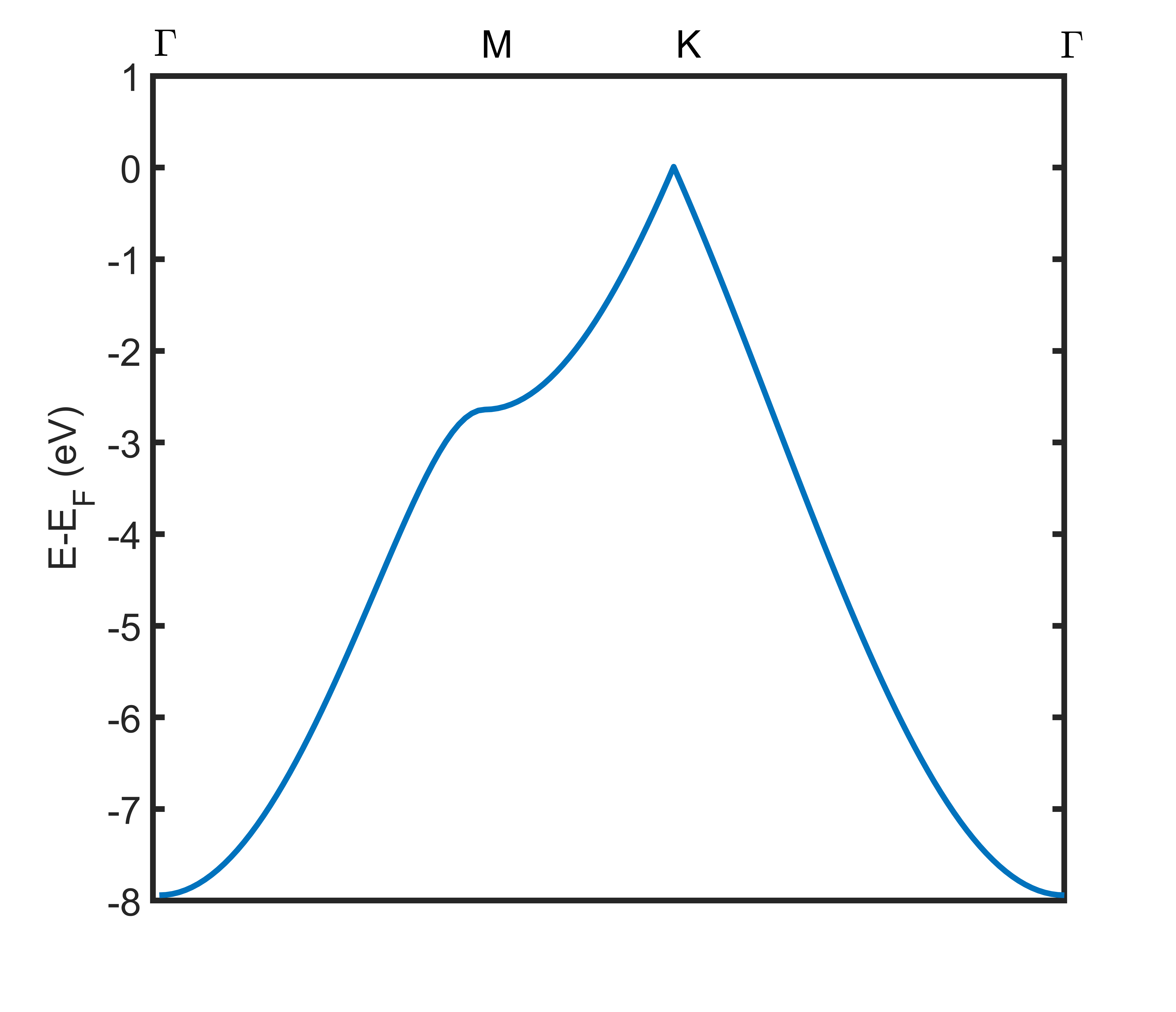
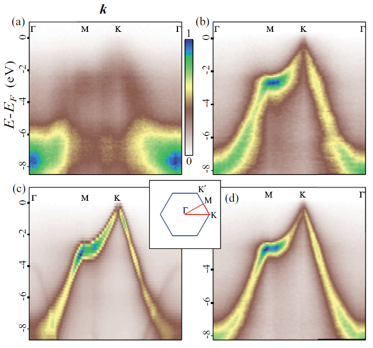
Here and are counterpart of and respectively corresponding to untwisted graphene layer i.e., for . electron per atom. We computed eigen values of for various values of parameters , , and . Computationally obtained quasi particle energy dispersion (shown in Figure:1a) fits best with experimentally observed dispersion(shown in Figure:1b) in monolayer graphene for eV, eV, eV, which agrees well with previously reported values [23].
In same basis as chosen for TBG, the Hamiltonian for AB-stacked bilayer graphene will have the form as given by equation 1bn.
| (1bn) |
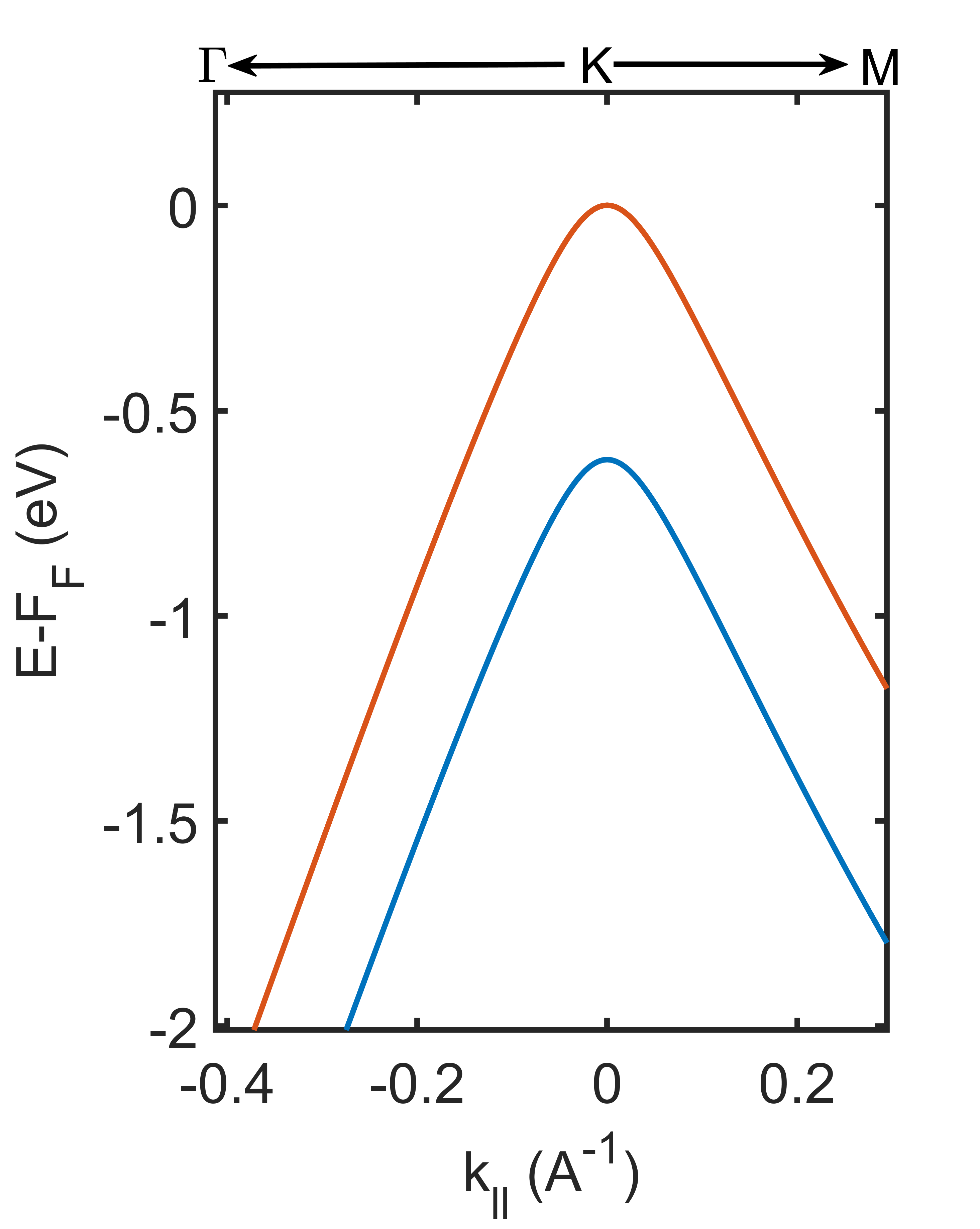
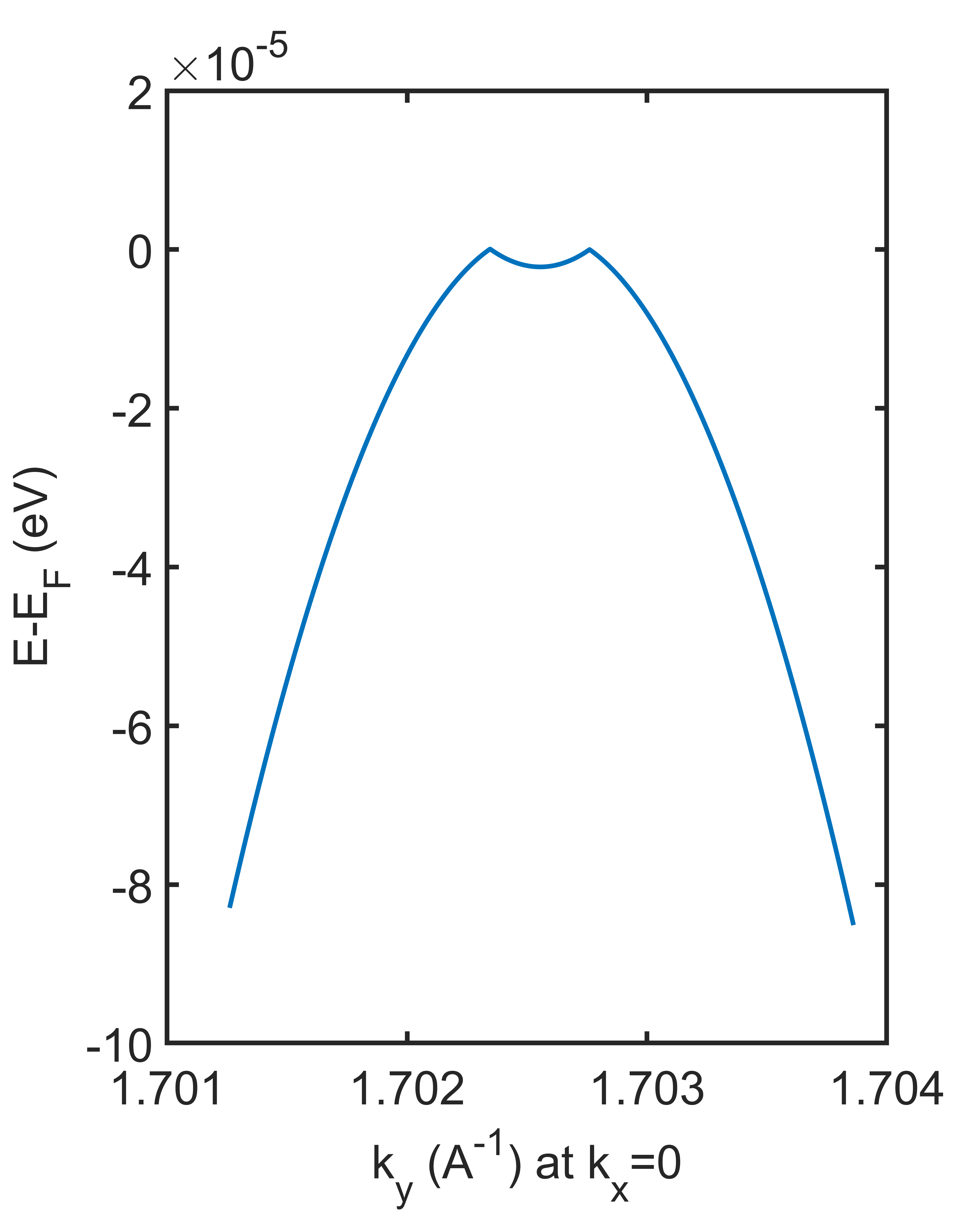
Here when ; when . We used eV, eV and eV, and computed eigen values of for various values of parameters and . Non zero values of change the dispersion at Dirac point from linear to parabolic. Change in changes the slope of dispersion at Dirac point and gap between two valence bands at Dirac point and this gap is almost equal to (shown in Figure:2a, 2c). Non zero values of insert a concave deformation in dispersion at Dirac point (shown in Figure:2b). Computationally obtained quasi particle energy dispersion (shown in Figure:2a) fits best with experimentally observed dispersion (shown in Figure:2c) in AB-stacked bilayer graphene for eV and eV.
eV suggests that interlayer hopping drops to zero when , therefore . Since range of inter-layer hopping () is small; after simulating the internal configurations of carbon atoms inside a supercell of TBG it becomes relatively easier to compute , , and for varying values of parameters , , , , and . After computing the values of , , and , eigen values of Hamiltonian are computed very easily. From eigen values of dispersion and density of states are obtained.

To estimate the values of parameters , , , , and we tried to simultaneously fit; the computed dispersion with experimentally observed dispersion in TBG with twist angle , the computed dispersion with experimentally observed dispersion in TBG with twist angle and the gap between two Van-Hove singularity peaks in computed density of states and experimentally observed tunnelling conductance in TBG with twist angle . Computationally obtained results fit best with experimentally observed results for , , , , and .
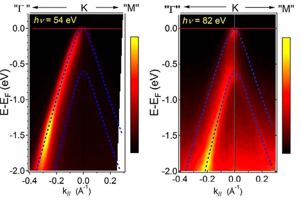
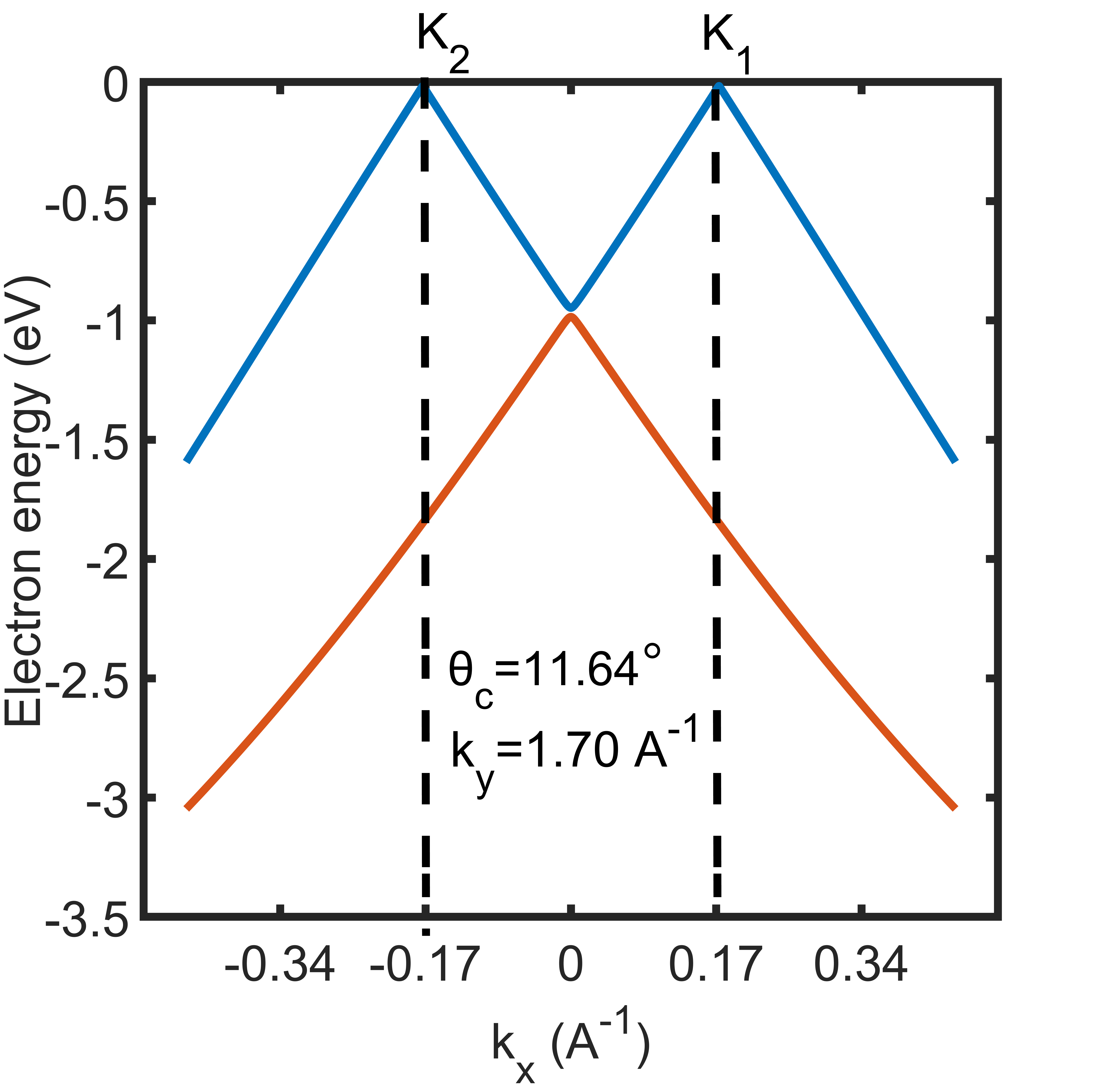
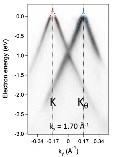
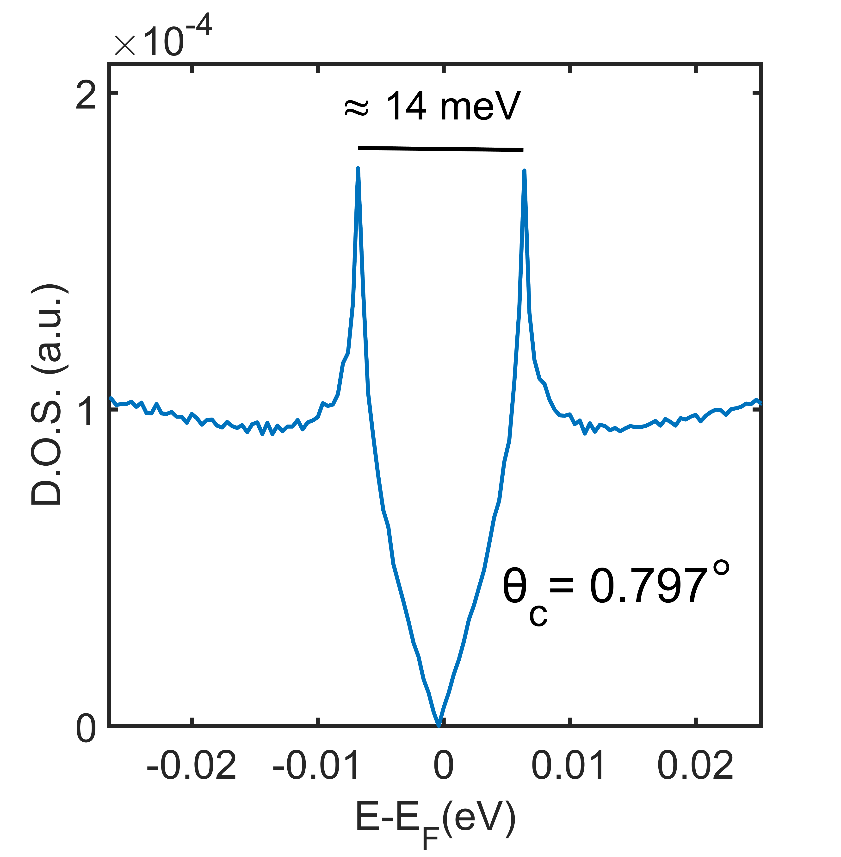
Figure 3a shows computed dispersion for TBG with twist angle , which is in good agreement with experimentally observed dispersion shown in Figure 3b. Figure 3b show experimentally observed dispersion for TBG with twist angle presented in FIG. 1(c) of reference [26]. Figure 3c shows computed dispersion for TBG with twist angle which is in good agreement with Fig:1(g), 2(c) of reference [14] showing experimentally observed dispersion for TBG with twist angle . Figure 3d shows computed D.O.S. for TBG with twist angle , the gap between two Van-Hove singularity peaks is in good agreement with Fig:2(c) of reference [9] showing experimentally observed gap between two Van-Hove singularity peaks for TBG with twist angle . After estimation of all parameters we computed electronic energy dispersion and D.O.S. for many TBG systems, some of those results are presented in following section.
5 Results and Discussion
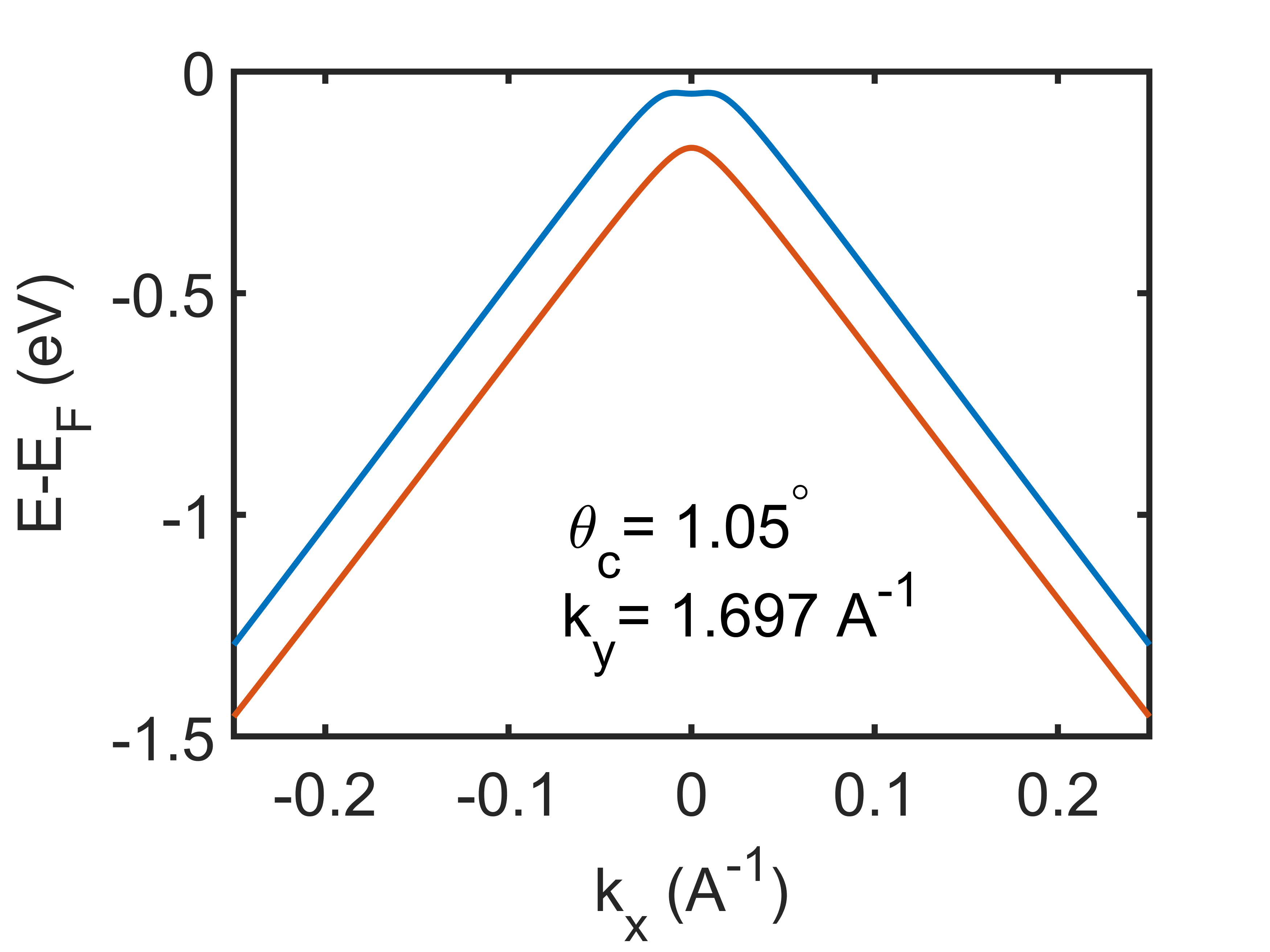

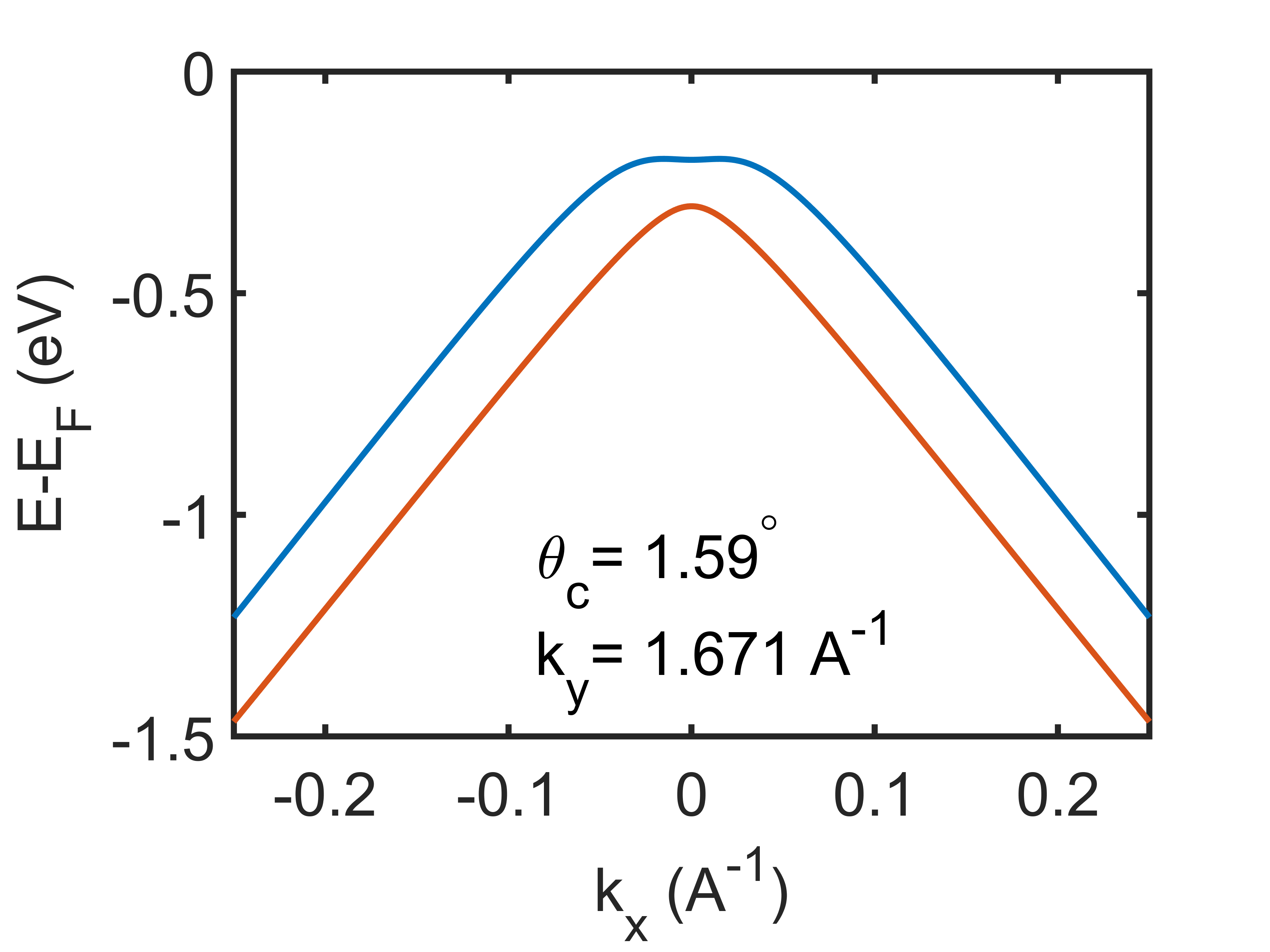
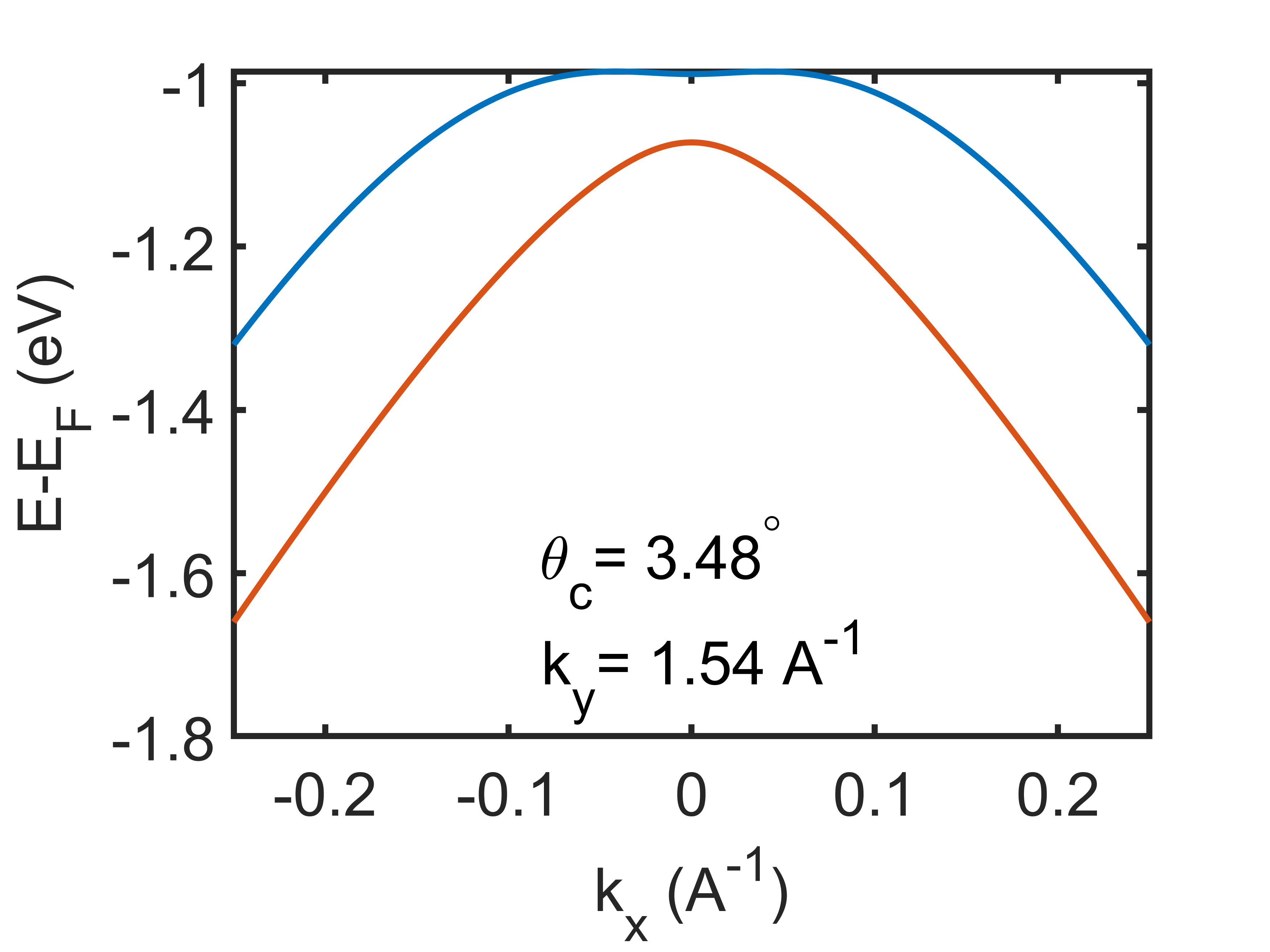
Figures 4a, 4b, 4c and 4d show computed quasi particle energy dispersion for TBG with twist angle , , and respectively, all show presence of flat band. For TBG with twist , flat band lies below of Fermi level, for TBG with twist , flat band lies below of Fermi level, for TBG with twist , flat band lies below of Fermi level and for TBG with twist , flat band lies below of Fermi level. As the twist angle increases, flat band move away from Fermi level. For TBG with twist , flat band occurs near , for TBG with twist , flat band occurs near , for TBG with twist , flat band occurs near and for TBG with twist , flat band occurs near . The coordinates of chosen Dirac point are . As the twist angle increases, flat band move away from Dirac point. As the twist angle increases sharpness of flat band decreases and the dispersion moves towards curved structure. computationally obtained band dispersion reveal that flat band in TBG occurs very close to Dirac point of graphene and only along linear dimension of two dimensional wave vector space parallel to line connecting two closest Dirac points of two graphene layers of TBG.
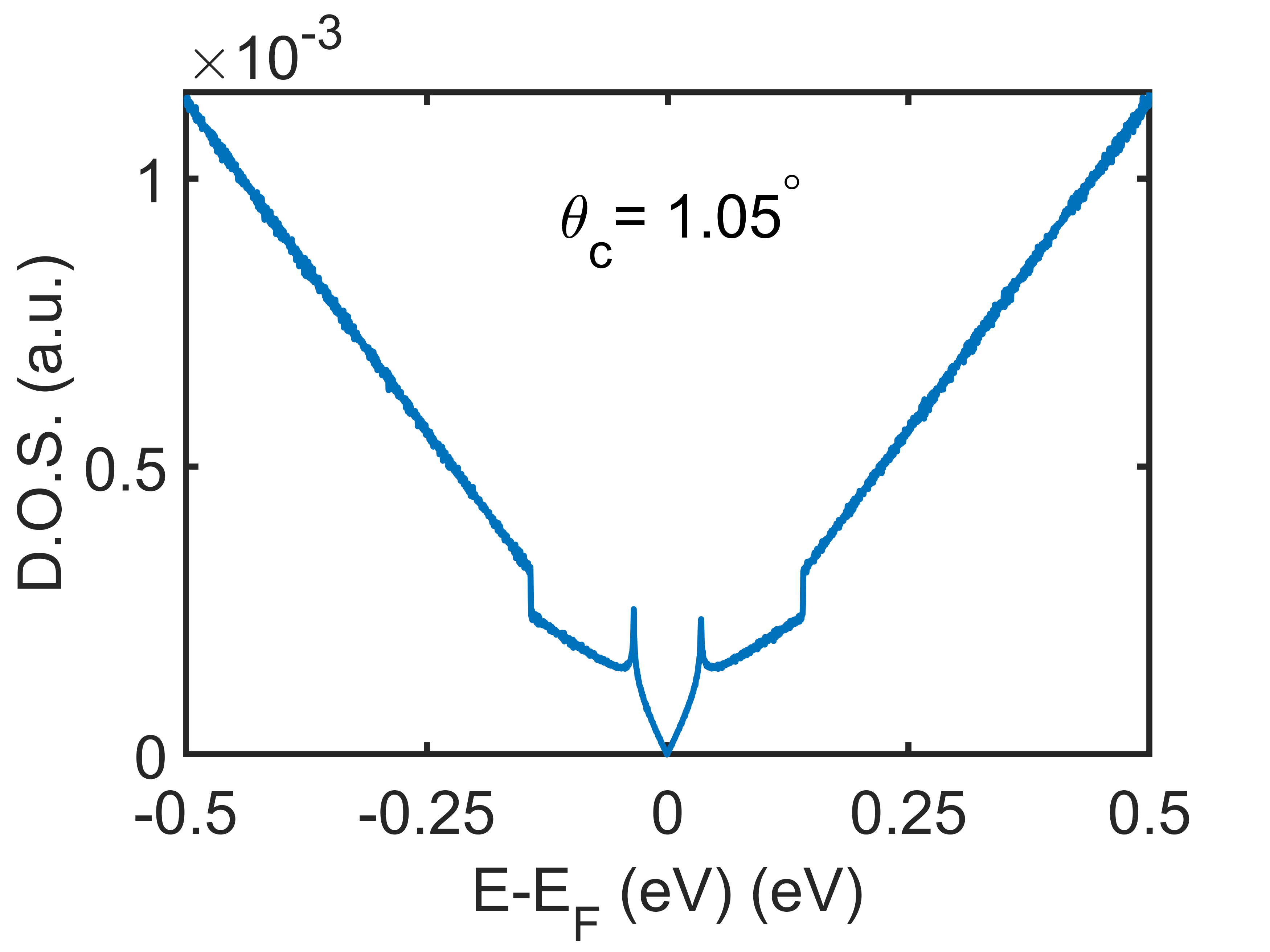
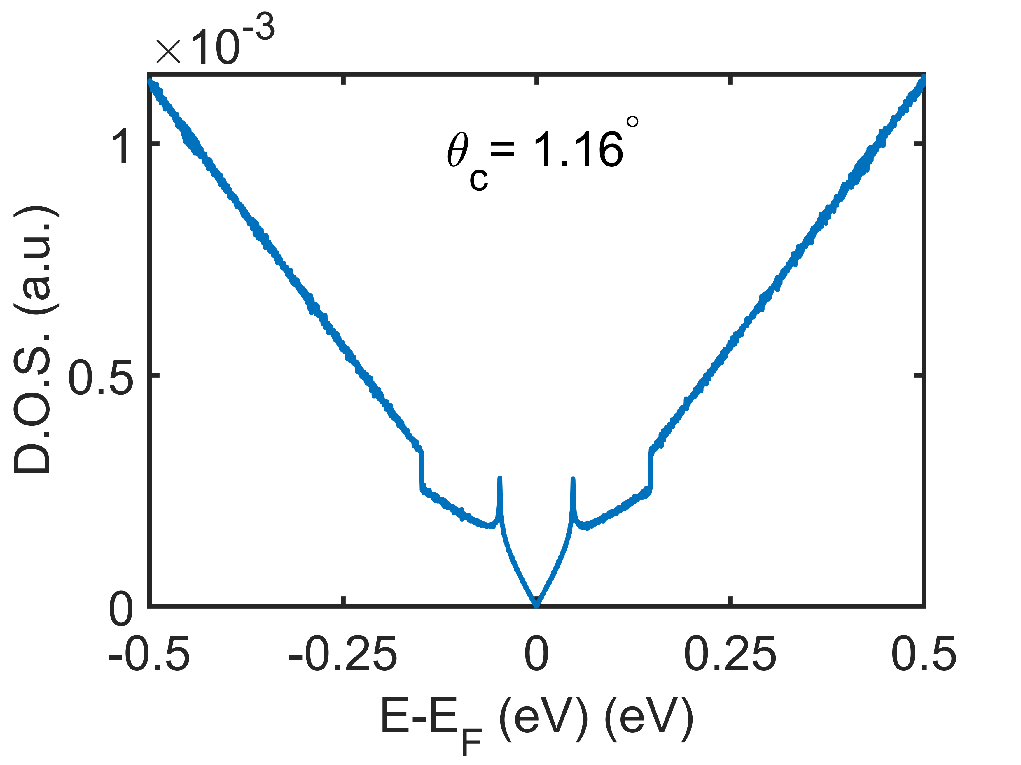
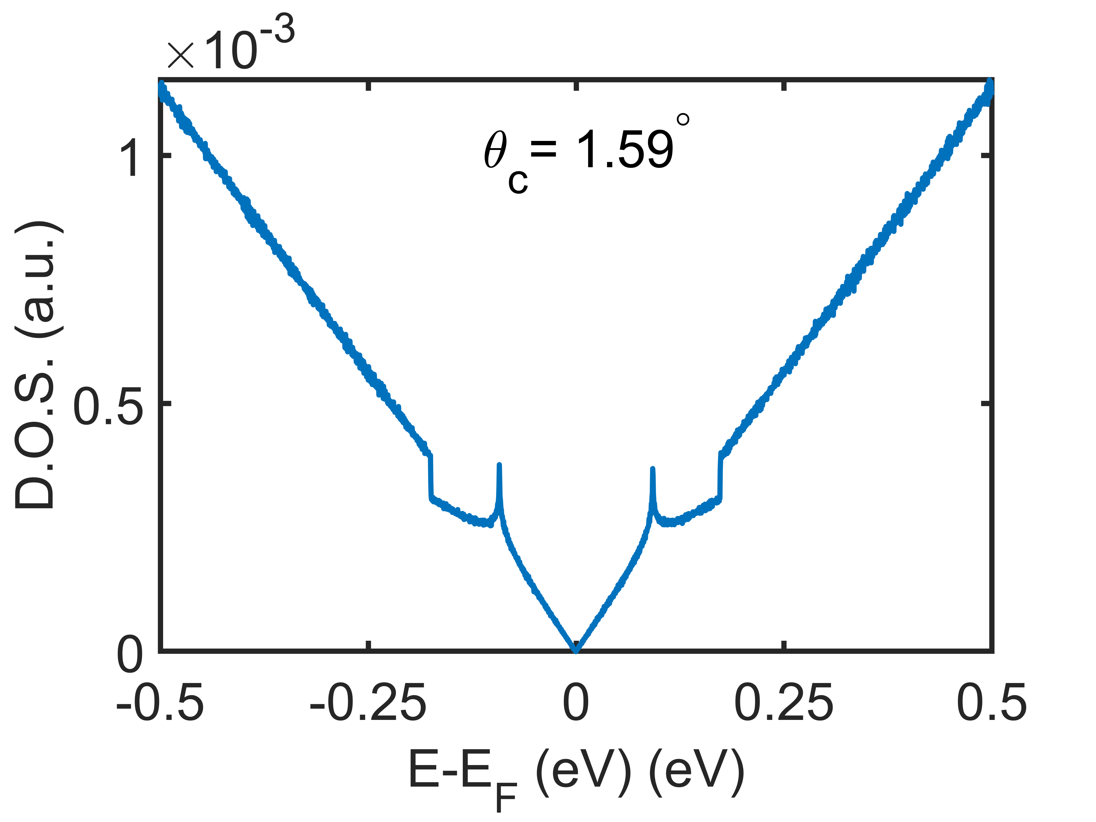

Figures 5a, 5b, 5c and 5d show computed electronic density of states for TBG with twist angle , , and respectively, all show presence of two Van-Hove singularity peaks near Fermi level. As the twist angle increases, Van-Hove singularity peaks move away from Fermi level and gap between two Van-Hove singularity peaks increases. This behaviour in consistent with behaviour of flat band. Computed dispersion and density of states for TBG show that instead of being restricted to TBG with discrete set of magic angles, flat band and Van-Hove singularities appear for all TBG systems having twist angle upto as observed experimentally. Even a simple tight binding Hamiltonian without electronic-correlations but with environment dependent interlayer hopping and incorporating complete internal configuration of carbon atoms inside a supercell can produce flat band dispersion and Van-Hove singularities near Fermi level for TBG. Flat band dispersion and Van-Hove singularities near Fermi gradually ruin as the twist angle increases. Shape of density of state near Fermi level indicate towards pseudo gap phase. Two Van-Hove singularities near Fermi level are consequence of two flat bands near Dirac points, one above Fermi level and other below Fermi level.
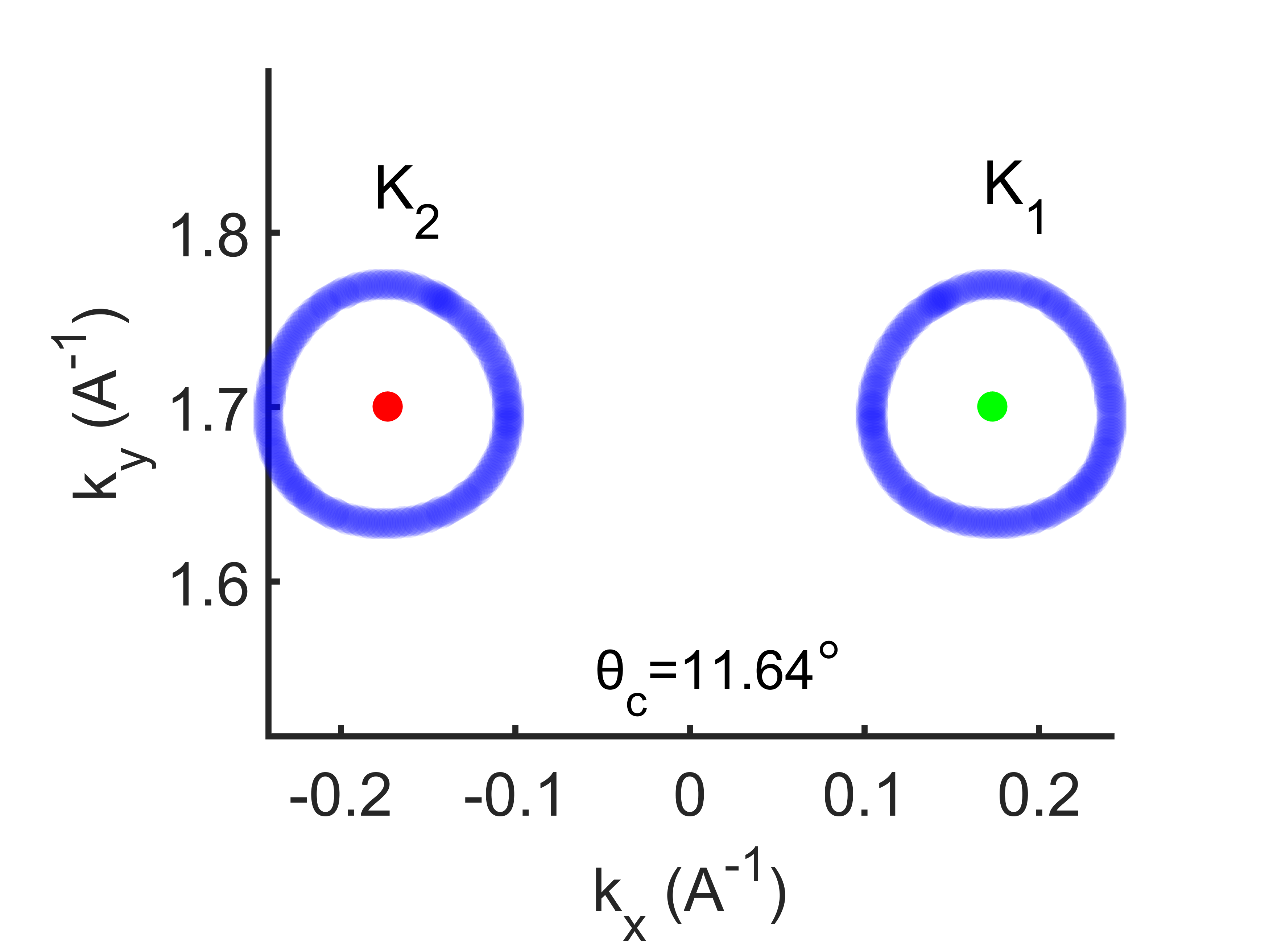

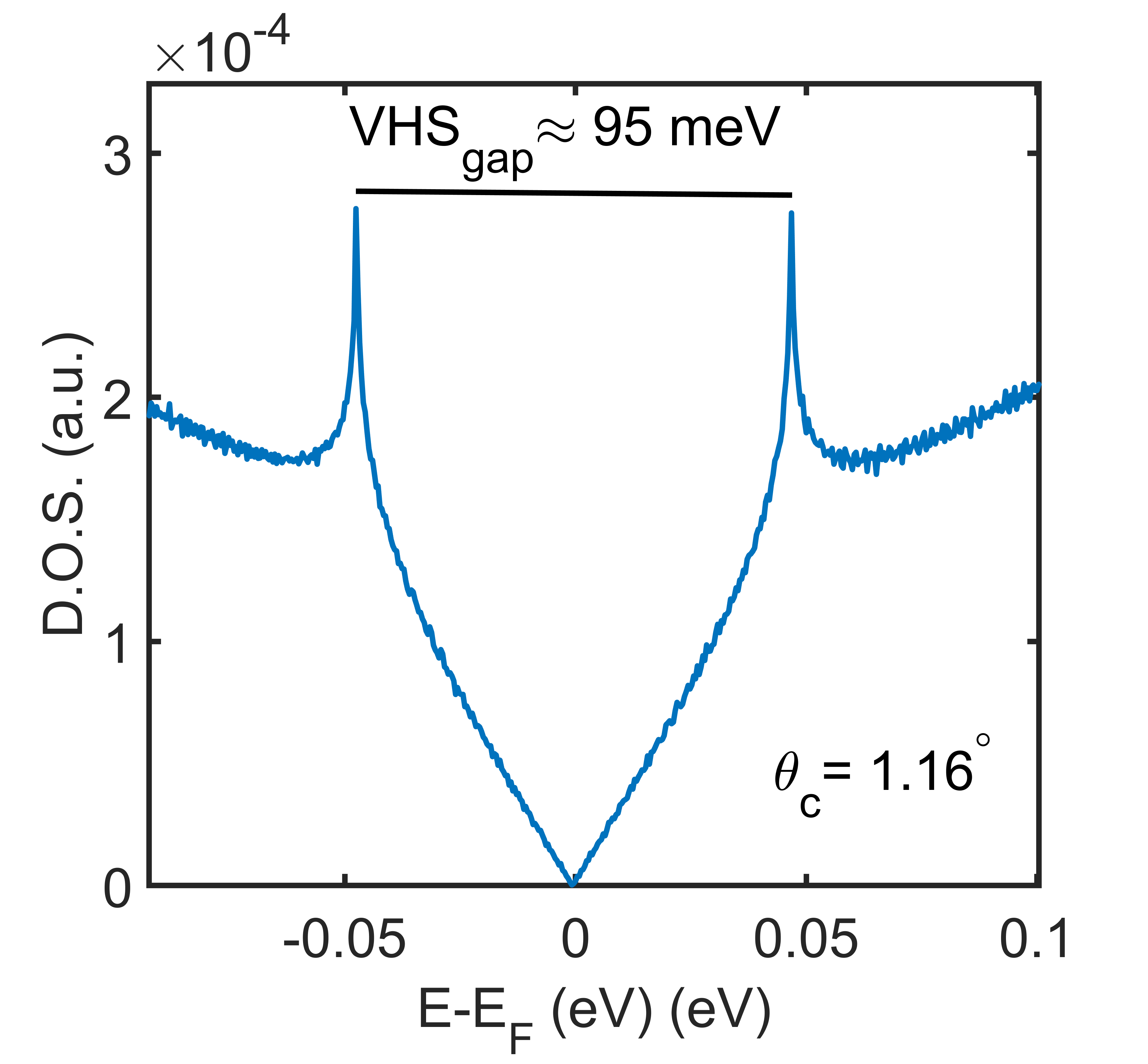
Figure 6a shows computed constant energy contour for TBG with twist angle at electron energy ; computed results are in good agreement with experimentally observed results presented in FIG. 1(b) of reference [26]. Figure 6b shows computed constant energy contour for TBG with twist angle at electron energy ; computed results differ significantly from experimentally observed results presented in Fig. 3(b) of reference [13]. Figure 6c shows gap between two Van-Hove singularity peaks in computed D.O.S. for TBG with twist angle . This gap between two Van-Hove singularity peaks in computed D.O.S. is which differ significantly from experimentally observed gap which is as reported in Fig. 2(c) of reference [9]. Another article of reference [5] reported this gap to be , indicating the inconsistency in available experimental data.
Computed results agree qualitatively and to a good extent quantitatively also with experimentally observed results. But for smaller twist angles this quantitative difference is significant. Theory considers ideal situation which does not take into account many experimental factors, this may cause significant difference in theoretical and experimental results. Other reason for difference between theoretical and experimental results may be absence of electronic correlations in theory which is firmly supported by scientific community [10, 16]. Inclusion of electronic correlations in theory and better approximation of environment dependent interlayer hopping function can further enhance the results.
References
References
- [1] Lopes dos Santos J M B, Peres N M R and Castro Neto A H 2007 Phys. Rev. Lett. 99(25) 256802 URL https://link.aps.org/doi/10.1103/PhysRevLett.99.256802
- [2] Shallcross S, Sharma S and Pankratov O A 2008 Phys. Rev. Lett. 101(5) 056803 URL https://link.aps.org/doi/10.1103/PhysRevLett.101.056803
- [3] Shallcross S, Sharma S, Kandelaki E and Pankratov O A 2010 Phys. Rev. B 81(16) 165105 URL https://link.aps.org/doi/10.1103/PhysRevB.81.165105
- [4] Lopes dos Santos J M B, Peres N M R and Castro Neto A H 2012 Phys. Rev. B 86(15) 155449 URL https://link.aps.org/doi/10.1103/PhysRevB.86.155449
- [5] Li G, Luican A, Lopes dos Santos J M B, Castro Neto A H, Reina A, Kong J and Andrei E Y 2010 Nature Physics 6(2) 109–113 URL https://doi.org/10.1038/nphys1463
- [6] Luican A, Li G, Reina A, Kong J, Nair R R, Novoselov K S, Geim A K and Andrei E Y 2011 Phys. Rev. Lett. 106(12) 126802 URL https://link.aps.org/doi/10.1103/PhysRevLett.106.126802
- [7] Bistritzer R and MacDonald A H 2011 PNAS 108(30) 12233–12237 URL https://doi/10.1073/pnas.1108174108
- [8] Cao Y, Fatemi V, Fang S, Watanabe K, Taniguchi T, Kaxiras E and Jarillo-Herrero P 2018 Nature 556(7699) 43–50 URL https://doi.org/10.1038/nature26160
- [9] Kerelsky A, McGilly L J, Kennes D M, Xian L, Yankowitz M, Chen S, Watanabe K, Taniguchi T, Hone J, Dean C, Rubio A and Pasupathy A N 2019 Nature 572(7767) 95–100 URL https://doi.org/10.1038/s41586-019-1431-9
- [10] Xie Y, Lian B, Jäck B, Liu X, Chiu C L, Watanabe K, Taniguchi T, Bernevig B A and Yazdani A 2019 Nature 572(7767) 101–105 URL https://doi.org/10.1038/s41586-019-1422-x
- [11] Choi Y, Kemmer J, Peng Y, Thomson A, Arora H, Polski R, Zhang Y, Zhang Y, Alicea J, Refael G, von Oppen F, Watanabe K, Taniguchi T and Nadj-Perge S 2019 Nature Physics 15(11) 1174–1180 URL https://doi.org/10.1038/s41567-019-0606-5
- [12] Jiang Y, Lai X, Watanabe K, Taniguchi T, Haule K, Mao J and Andrei E Y 2019 Nature 573(7772) 91–95 URL https://doi.org/10.1038/s41586-019-1460-4
- [13] Lisi S, Lu X, Benschop T, de Jong T A, Stepanov P, Duran J R, Margot F, Cucchi I, Cappelli E, Hunter A, Tamai A, Kandyba V, Giampietri A, Barinov A, Jobst J, Stalman V, Leeuwenhoek M, Watanabe K, Taniguchi T, Rademaker L, van der Molen S J, Allan M P, Efetov D K and Baumberger F 2021 Nature Physics 17(2) 189–193 URL https://doi.org/10.1038/s41567-020-01041-x
- [14] Utama M I B, Koch R J, Lee K, Leconte N, Li H, Zhao S, Jiang L, Zhu J, Watanabe K, Taniguchi T, Ashby P D, Weber-Bargioni A, Zettl A, Jozwiak C, Jung J, Rotenberg E, Bostwick A and Wang F 2020 Nature Physics 17(2) 184–188 URL https://doi.org/10.1038/s41567-020-0974-x
- [15] Yankowitz M, Chen S, Polshyn H, Zhang Y, Watanabe Kand Taniguchi T G D, Young A F and Dean C R 2019 Science 363 1059–1064 URL https://www.science.org/doi/abs/10.1126/science.aav1910
- [16] Oh M, Nuckolls K P, Wong D, Lee R L, Liu X, Watanabe K, Taniguchi T and Yazdani A 2021 Nature 600(7888) 240–245 URL https://doi.org/10.1038/s41586-021-04121-x
- [17] Cao Y, Fatemi V, Demir A, Fang S, Tomarken S L, Luo J Y, Sanchez-Yamagishi J D, Watanabe K, Taniguchi T, Kaxiras E, Ashoori R C and Jarillo-Herrero P 2018 Nature 556(7699) 80–86 URL https://doi.org/10.1038/nature26154
- [18] Tseng C C, Ma X, Liu Z, Watanabe K, Taniguchi T, Chu J H and Yankowitz M 2022 Nature Physics 18(9) 1038–1042
- [19] Lin J X, Zhang Y H, Morissette E, Wang Z, Liu S, Rhodes D, Watanabe K, Taniguchi T, Hone J and Li J I A 2022 Science 375 437–441 (Preprint https://www.science.org/doi/pdf/10.1126/science.abh2889) URL https://www.science.org/doi/abs/10.1126/science.abh2889
- [20] Benlakhouy N, Jellal A, Bahlouli H and Vogl M 2022 Phys. Rev. B 105(12) 125423 URL https://link.aps.org/doi/10.1103/PhysRevB.105.125423
- [21] Veerpal and Ajay arXiv.org URL https://doi.org/10.48550/arXiv.2302.09617
- [22] Yin Y, Cheng Z, Wang L, Jin K and Wang W 2014 Scientific Reports 4(1) 5758 URL https://doi.org/10.1038/srep05758
- [23] Wehling T O, Şaşıoğlu E, Friedrich C, Lichtenstein A I, Katsnelson M I and Blügel S 2011 Phys. Rev. Lett. 106(23) 236805 URL https://link.aps.org/doi/10.1103/PhysRevLett.106.236805
- [24] Knox K R, Locatelli A, Yilmaz M B, Cvetko D, Menteş T O, Niño M A, Kim P, Morgante A and Osgood R M 2011 Phys. Rev. B 84(11) 115401 URL https://link.aps.org/doi/10.1103/PhysRevB.84.115401
- [25] Cheng C M, Xie L, Pachoud A, Moser H, Chen W, Wee A, Castro Neto A, Tsuei K D and Özyilmaz B 2015 Scientific Reports 5(1) 10025 URL https://doi.org/10.1038/srep10025
- [26] Ohta T, Robinson J T, Feibelman P J, Bostwick A, Rotenberg E and Beechem T E 2012 Phys. Rev. Lett. 109(18) 186807 URL https://link.aps.org/doi/10.1103/PhysRevLett.109.186807