Magnetic plateaus and jumps in a spin-1/2 ladder with alternate Ising-Heisenberg rungs: a field dependent study

Abstract

We study a frustrated two-leg spin-1/2 ladder with alternate Ising and isotropic Heisenberg rung exchange interactions, whereas, interactions along legs and diagonals are Ising type. The ground-state (GS) of this model has four exotic phases: (i) the stripe-rung ferromagnet (SRFM), (ii) the anisotropic anti-ferromagnet (AAFM), (iii) the Dimer, and (iv) the stripe-leg ferromagnet (SLFM) in absence of any external magnetic field. In this work, the effect of externally applied longitudinal and transverse fields on quantum phases is studied. In both cases, we show that there exist two plateau phases at $1/4$, and $1/2$ of the saturation of magnetization. Due to the strong rung dimer formation, the system opens a finite spin gap for all the phases resulting in a zero magnetization plateau in the presence of a longitudinal field. The mechanism of plateau formation is analyzed using spin density, quantum fidelity, and quantum concurrence. In the (i) SRFM phase, Ising exchanges are dominant for all spins but the Heisenberg rungs are weak, and therefore, the magnetization shows a continuous transition as a function of the transverse field. In the other three phases [(ii)-(iv)], Ising dimer rungs are weak and broken first to reach the plateau at $1/2$ of the saturation magnetization, having a large gap, which is closed by further application of the field. We use the exact diagonalization (ED) and the transfer matrix method (TM) to solve the Hamiltonian.

I Introduction

Frustrated low-dimensional quantum magnets exhibit a zoo of quantum phases which attracts more interest to both theoreticians as well as experimentalists, and so the theoretical studies are quite necessary for the verification of the experimental results due to the ever-growing synthesis of low-dimensional magnetic materials Nakamura and Okamoto (1998); Guo et al. (2020); Kakarla et al. (2021); Dagotto and Rice (1996); Chubukov (1991); Chubukov et al. (1994); Hutchings M T (1979); Park et al. (2007); Mourigal et al. (2012); Drechsler et al. (2007); Dutton et al. (2012a, b); Maeshima et al. (2003); Sandvik et al. (1996); Johnston et al. (1987). In the spin chains and ladder systems, the competing exchange interactions lead to many interesting quantum phases like ferromagnetic ground state Vekua et al. (2003), Néel phase Richter et al. (2004); Ogino et al. (2021, 2022), Luttinger liquid Luttinger (1963); Sakai et al. (2022), spiral Maiti and Kumar (2019), spin liquid Balents (2010); Liao et al. (2017), dimer phase Dagotto and Rice (1996), etc. The ground state (GS) of antiferromagnetic isotropic Heisenberg spin-1/2 zigzag chain has a gapless spectrum in small or strong coupling limit, whereas, it has a gapped spectrum for the moderate value of the ratio of the exchange interactions Barnes et al. (1993); Johnston et al. (2011); Kumar et al. (2015); Chitra et al. (1995); White and Affleck (1996); Rahaman et al. (2023).

In a non-frustrated regime i.e, for the weak and strong rung isotropic exchange limit, the GS is in a spin liquid state with quasi-long range order (QLRO) and gapless spectrum Chitra et al. (1995); White and Affleck (1996). Whereas, in the presence of anisotropic exchanges, it is gapped if axial exchange term Z is dominant, otherwise, gapless if XY term dominates, and, the anisotropic Heisenberg spin-1/2 chain is its one of the best examples Rakov et al. (2016); Mikeska and Kolezhuk (2004). The GS of spin-1/2 normal ladder with isotropic Heisenberg exchange is always gapped irrespective of the strength of the rung exchange but it may have a gapless spectrum for the anisotropic ladder systems Wessel et al. (2017); Morita et al. (2015); Hijii et al. (2005); Mikeska and Kolezhuk (2004); Agrapidis et al. (2019); Liu et al. (2022); Li et al. (2017). As an example, having an isotropic exchange in the rung and axial anisotropy $\Delta$ along the leg, the GS can be tuned from singlet to Néel phase by increasing $\Delta$ Hijii et al. (2005). In case having anisotropy on both: leg and rung exchange interactions, the GS can be XY, Néel, or rung singlet (RS) phase on tuning the rung exchange and axial anisotropy Li et al. (2017). Another type of anisotropic spin-1/2 ladder is the Kitaev-Heisenberg model on a two leg ladder where the GS has many exotic quantum phases Agrapidis et al. (2019).

Many spin-1/2 ladder systems with isotropic and anisotropic exchange interactions have been extensively studied under magnetic field and are reported to exhibit some of the magnetic plateaus and jumps Ivanov (2009); Sakai and Yamamoto (1999); Sakai and Okazaki (2000); Naseri and Mahdavifar (2017); Zad and Ananikian (2018); Japaridze and Pogosyan (2006a); Moradmard et al. (2014); Dey et al. (2020); Oshikawa et al. (1997); Strecka and Jascur (2003); Strečka et al. (2014); Verkholyak and Strečka (2012); Verkholyak and Strecka (2013); Karl’ová et al. (2019). Japaridze et al. studied a two-leg spin-$\frac{1}{2}$ ladder system with leg interaction $J_{\parallel}$ and alternate rung as $J_{\perp}^{+}$, $J_{\perp}^{-}$ in presence of a longitudinal field $h$. They have shown that the system shows a zero magnetization up to $h_{c1}^{-}$, a plateau at half of the saturation magnetization between $h_{c1}^{+}$ and $h_{c2}^{-}$ and full saturation achieved at $h_{c2}^{+}$ Japaridze and Pogosyan (2006b). Moradmard et al. studied a spin-1/2 ladder system with XXZ interaction and they have shown different phases like x-FM, z-FM, y-Néel, and z-Néel in a magnetic phase diagram in the plane of anisotropy interaction $\Delta$ and magnetic field $h$ Moradmard et al. (2014). Similarly, Dey et.al. carried out the magnetization study of isotropic Heisenberg spin-1/2 on a 5/7-skewed ladder and showed multiple plateau phases with field $h$ Dey et al. (2020). They show that plateau phases are the consequences of gaps in the spectrum, and these plateau phases can be explained in terms of Oshikawa, Yamanaka, and Affleck (OYA) criterion Oshikawa et al. (1997). Some of the rigorous studies on special types of ladders having the Ising-Heisenberg exchange interactions report the magnetization process in various GS phases Strecka and Jascur (2003); Strečka et al. (2014, 2014); Verkholyak and Strečka (2012); Verkholyak and Strecka (2013); Karl’ová et al. (2019). For a spin-$1/2$ two-leg ladder with Ising type leg, diagonal, and Heisenberg type rung exchange interaction, Verkholayak et. al. find that a Néel ordered GS phase undergoes a phase transition to full saturation of the magnetization through a $1/2$ of the saturation, namely staggered bond (SB) phase in presence of an external field Verkholyak and Strečka (2012). For a spin-1/2 Ising-Heisenberg branched chain, it is shown that the magnetization curve shows a plateau at the half saturation which can be characterized by quantum concurrence as well Karl’ová et al. (2019).

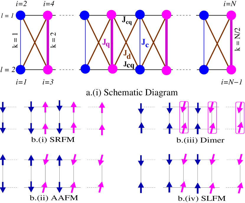
Figure 1: (color online) a.(i) Schematic diagram of the spin ladder with alternate Ising-Heisenberg rung interactions. $J_{c}$ and $J_{q}$ are the alternative Ising and Heisenberg type rung interactions respectively. $J_{cq}$, $J_{d}$ are the Ising type leg and diagonal exchange interactions respectively. Blue and magenta color circles represent $\sigma$ and S spins in Eq.II respectively. $l$, $k$, and $i$ represent leg and rung, and site indices respectively. The spin configurations of four exotic phases with $J_{c}=J_{cq}=1$: b.(i) SRFM ($J_{q}=0.2$, $J_{d}=2.0$), b.(ii) AAFM ($J_{q}=2.0$, $J_{d}=0.4$), b.(iii) Dimer ($J_{q}=2.0$, $J_{d}=1.0$), and b.(iv) SLFM ($J_{q}=2.0$, $J_{d}=1.6$) are shown. Blue and magenta rung pairs are representing $\sigma-\sigma$ and $S-S$ rung pairs. The boxes shown in Subfigure b.(iii) represent perfect singlets. Quantum phases are studied earlier in Ref. Rahaman et al. (2021).

We consider a spin-1/2 frustrated two-leg ladder system with alternating Ising and Heisenberg type rung exchanges, where the diagonal and leg exchange are of Ising type as shown in Fig.1.a.i. In this model, $J_{c}$ and $J_{q}$ are the alternate Ising and Heisenberg rung exchange interactions respectively, where, $J_{cq}$ and $J_{d}$ are the leg and diagonal exchange interaction strengths of Ising type respectively. The quantum phase diagram of this model is studied earlier in parameter space of $J_{q}$ and $J_{d}$ (both are antiferromagnetic) by considering $J_{c}=J_{cq}=1$ Rahaman et al. (2021). The system exhibits four distinct GS phases under periodic boundary condition (PBC): (i) stripe rung ferromagnet (SRFM), (ii) the anisotropic antiferromagnet (AAFM), (iii) the Dimer, and (iv) the stripe leg ferromagnet (SLFM) depending upon the values of $J_{q}$ and $J_{d}$ in absence of any magnetic field Rahaman et al. (2021). The GS phases are schematically represented in Fig1.b.[(i)-(iv)]. In this manuscript, we study the effect of both axial or longitudinal and transverse magnetic fields on the four GS phases with a few sets of $J_{q}$, $J_{d}$ values discussed in Sec.IV.

In this work, we observe that in all the quantum phases, the system exhibits a plateau at zero, half, and full of saturation magnetization in the presence of an externally applied longitudinal magnetic field. The calculations are done using the exact diagonalization (ED) ER (1975) and transfer matrix (TM) Suzuki (1985) methods, and results from both methods agree excellently with each other. Furthermore, we calculate the zero-temperature limit quantum fidelity, fidelity susceptibility, and quantum concurrence from the partition function of the ladder using TM, and find that these results are in accordance with the exact calculation. The study of the magnetization under a transverse field is carried out using ED only, and it is noticed that the magnetization shows a half, and full of saturation magnetization plateaus.

This paper is divided into a few sections as follows. First, the model is discussed briefly in Sec. II. This is followed by a discussion on methods in Sec. III. The Sec. IV has two subsections dedicated to the study in the presence of a magnetic field along two directions: longitudinal and transverse. In Sec. IV.1.1, the magnetization process is discussed in the presence of the longitudinal field. In Sec. IV.1.2, we discuss the zero-temperature limit quantum fidelity and bipartite concurrence for different phases. In Sec. IV.2, we discuss the magnetization process in the presence of a transverse field. In Sec. V, we summarise the results and conclude the paper.

II Model Hamiltonian

We construct the Hamiltonian for a spin-1/2 two-leg ladder with $N$ number of spins periodically connected along the leg, which turns out to be comprised of $n=\frac{N}{4}$ number of unit cells. In each unit cell, one rung pair is connected through an Ising type exchange $J_{c}$, whereas, the other one is coupled with a Heisenberg type exchange $J_{q}$ as shown in Fig.1. These rungs couple each other through Ising type exchanges: $J_{cq}$ along the leg, $J_{d}$ along the diagonal. The spins with rung coupling $J_{c}$ and $J_{q}$ are marked with $\sigma$ and $\vec{S}$ respectively. Here onward, the Ising type and Heisenberg type rung spin pairs are to be called $\sigma-\sigma$ and $S-S$ pairs respectively. Let us now write down the Hamiltonian for one unit cell-

$$\mathbf{H_{i}}=J_{q}\vec{S}_{2i,1}\cdot\vec{S}_{2i,2}+\frac{J_{c}}{2}[\sigma_{2i-1,1}\sigma_{2i-1,2}+\sigma_{2i+1,1}\sigma_{2i+1,2}]$$

$$+J_{cq}[S_{2i,1}^{z}(\sigma_{2i-1,1}+\sigma_{2i+1,1})+S_{2i,2}^{z}(\sigma_{2i-1,2}+\sigma_{2i+1,2})]$$

$$+J_{d}[S_{2i,1}^{z}(\sigma_{2i-1,2}+\sigma_{2i+1,2})+S_{2i,2}^{z}(\sigma_{2i-1,1}+\sigma_{2i+1,1})]$$

$$-\frac{h}{2}\sum_{l=1}^{2}(2S_{2i,l}^{z}+\sigma_{2i-1,l}+\sigma_{2i+1,l})$$

$$-\frac{h^{x}}{2}\sum_{l=1}^{2}(2S_{2i,l}^{x}+\sigma_{2i-1,l}^{x}+\sigma_{2i+1,l}^{x})$$ (1)

Here, $h$ and $h^{x}$ are the longitudinal (+z direction) and transverse ( +x direction) fields respectively. The general Hamiltonian under PBC for a finite size ladder is the summation of the $n$ unit cells, which can be written as $\mathbf{H}=\sum_{i=1}^{n}\mathbf{H_{i}}$.

III Methods

We employ the ED method to solve the energy eigenvalues and eigenvectors of the Hamiltonian in Eq.II for the system sizes $N=16,20,24$ in the presence of longitudinal and transverse fields both. Whereas, in the absence of a transverse field i.e., for $h^{x}=0$, the Hamiltonian of two consecutive units commute to each other, and so we employ the TM method to calculate the magnetization, quantum fidelity, quantum concurrence from free energy, and partition function. The partition function for the entire system of system size $N$ can be written as $Q_{N}(h,\beta)=Tr(e^{-\beta\mathbf{H}})=[Q_{4}(h,\beta)]^{n}$ (see appendix VII). $Q_{4}(h,\beta)$ is the partition function for one small unit of 4 spins and $\beta$ is the inverse temperature. For this model, $Q_{N}(h,\beta)=[\lambda_{1}+\lambda_{2}+\lambda_{3}+\lambda_{4}]^{n}$ , where, $\lambda_{1},\lambda_{2},\lambda_{3},\lambda_{4}$ are the eigenvalues of a $4\times 4$ transfer matrix for one unit (see appendix VII). In the limit $n\rightarrow\infty$, and with the condition $\lambda_{1}\gg\lambda_{2}\gg\lambda_{3}\gg\lambda_{4}$, one can write $Q_{N}(h,\beta)\approx\lambda_{1}^{n}$ and $Q_{4}(h,\beta)\approx\lambda_{1}$. At zero-temperature limit i.e., for $\beta\rightarrow\infty$, after defining some of the system parameters: $\Delta_{2}=\sqrt{1+4(\frac{1-J_{d}}{J_{q}})^{2}}$, $Q=e^{\beta J_{q}/4}$, we obtain the partition function $Q_{4}(h,\beta)$

$$=e^{\frac{-\beta(J_{c}-4h)}{4}}\bigg{[}Q^{-1}cosh[\beta(h-1-J_{d})]+Qcosh[\frac{\beta J_{q}}{2}]\bigg{]}$$

$$+e^{\frac{\beta J_{c}}{4}}\bigg{[}2Q^{-1}cosh[\beta h]+Qcosh[\frac{\beta J_{q}\Delta_{2}}{2}]+Qcosh[\frac{\beta J_{q}}{2}]\bigg{]}$$ (2)

We rewrite $Q_{4}(h,\beta)$ as a polynomial function of $e^{\beta h}$:

$$Q_{4}(h,\beta)=a_{0}e^{2\beta h}+b_{0}e^{\beta h}+c_{0}e^{-\beta h}+d_{0}$$ (3)

Where, the coefficients of the polynomial are defined as:
$a_{0}=e^{-\frac{\beta}{4}(J_{q}+J_{d}+2)}$,
$b_{0}=2e^{-\frac{\beta}{4}(J_{q}-1)}+2e^{\frac{\beta}{4}(J_{q}-1)}Cosh[\frac{\beta J_{q}}{2}]$,
$c_{0}=2e^{-\frac{\beta}{4}(J_{q}-1)}$
$d_{0}=2Cosh[\frac{\beta J_{q}}{2}](e^{\frac{\beta J_{q}}{4}}+e^{\frac{-\beta}{4}})+2e^{\frac{\beta J_{q}}{4}}Cosh[\frac{\beta J_{q}\Delta_{2}}{2}]+e^{\frac{\beta(7+8J_{d}+J_{q})}{4}}$

IV Results

We study the magnetization properties for four sets of exchange parameters: (i) $J_{q}=0.2,J_{d}=2.0$ for the SRFM, (ii) $J_{q}=2.0,J_{d}=0.4$ for the AAFM, (iii) $J_{q}=2.0,J_{d}=1.0$ for the Dimer, and (iv) $J_{q}=2.0,J_{d}=1.6$ for the SLFM phases. It is to be mentioned that in all these phases, $J_{c}$ and $J_{cq}$ are unity.

IV.1 Magnetization process in the presence of a longitudinal magnetic field

IV.1.1 Magnetization vs field

To calculate the magnetization using ED, we first define the spin gap $\Gamma_{k_{1},k_{2}}$ which is the difference between the lowest energies $E_{0}(k_{1})$ and $E_{0}(k_{2})$ of two spin sectors $S^{z}=k_{1}$, $S^{z}=k_{2}$ respectively, and can be written as

$$\Gamma_{k_{1},k_{2}}=E_{0}(k_{2})-E_{0}(k_{1})$$ (4)

$S^{z}_{k}$ is the z component of the total spin in spin sector $k$ for the entire ladder. The per-site magnetization is calculated as $m=k/N$. This energy gap can be closed i.e, $h|k_{2}-k_{1}|=|\Gamma_{k_{1},k_{2}}|$ by applying a longitudinal field $h$. For spin-1/2 systems, $m$ takes the value between $0$ and $1/2$. Using the TM method, the per-site magnetization is obtained as $m=-\frac{\partial F(h,\beta)}{\partial h}$, where $F(h,\beta)$ is the free energy (see Appendix VII).

Figure 2: (PBC) Black, red, and green colors are the magnetization per site in the presence of a longitudinal field $h$ for the system sizes $N=16,20,24$ using ED. The blue color represents the magnetization calculated using the TM method at $T/J_{c}\rightarrow 0$. The values of $J_{q}$, $J_{d}$ are (i) $0.2,2.0$ for the SRFM, (ii) $2.0,0.4$ for the AAFM, (iii) $2.0,1.0$ for the Dimer, and (iv) $2.0,1.6$ for the SLFM phases respectively.

In Fig.2[(i)-(iv)], we show the finite size scaling of the m-h curve for three system sizes $N=16,20,24$ using ED and also for the thermodynamic limit ($N\rightarrow\infty$) in zero-temperature limit using TM. $m-h$ curve shows three plateau phases: $m=0,1/4$, and $1/2$ connected by two magnetic jumps in each of the subfigures. The first jump is at $h_{c1}$ from $m=0$ to $1/4$, and the other at $h_{c2}$ from $m=1/4$ to full saturation of magnetization in all four quantum phases as shown in Fig.2[(i)-(iv)]. The $h_{c1}$ takes values 2.5, 0.7, 0.5, and 0.7, and $h_{c2}$ is 3.5, 3.5, 4, 4.5 for (i) the SRFM, (ii) the AAFM, (iii) the Dimer, and (iv) the SLFM phases respectively. Later on, we discuss in detail that these magnetic transitions show plateaus due to the spin gap and the jumps correspond to unbinding of the rung dimers of equal energy. It is noticed that there is no finite size effect in the magnetization curve.

In the stationary condition, the differentiation of free energy with respect to magnetization is always zero i.e, $\frac{\partial{F(h,\beta)}}{\partial{m}}=0$ (followed from Eq.17). Using this condition, we find two critical fields $h_{c_{1}}=h_{-}$, $h_{c_{2}}=h_{+}$

$$h_{\pm}=\frac{1}{\beta}ln\big{[}\frac{b_{0}\pm\sqrt{b^{2}_{0}-3a_{0}d_{0}}}{3a_{0}}\big{]}$$ (5)

Since, $a_{0}=e^{-\frac{\beta}{4}(J_{q}+J_{d}+2)}$ is negligibly small for $\beta\rightarrow\infty$, one can consider $b_{0}^{2}\gg 3a_{0}d_{0}$ and can take the binomial expansion of the square root term in the above equation. This leads to writing down the critical fields approximately as $h_{c1}=\frac{1}{\beta}ln\left[\frac{d_{0}}{2b_{0}}\right]$ and $h_{c2}=\frac{1}{\beta}ln\left[\frac{2b_{0}}{3a_{0}}\right]$ in zero temperature limit . These critical fields are found to be matching with the exact calculations discussed above and shown in the $m-h$ curve in Fig.2. Plateau width can be obtained as

$$d=|h_{c2}-h{c1}|=\frac{1}{\beta}ln\left[\frac{4b_{0}^{2}}{3a_{0}d_{0}}\right]$$ (6)

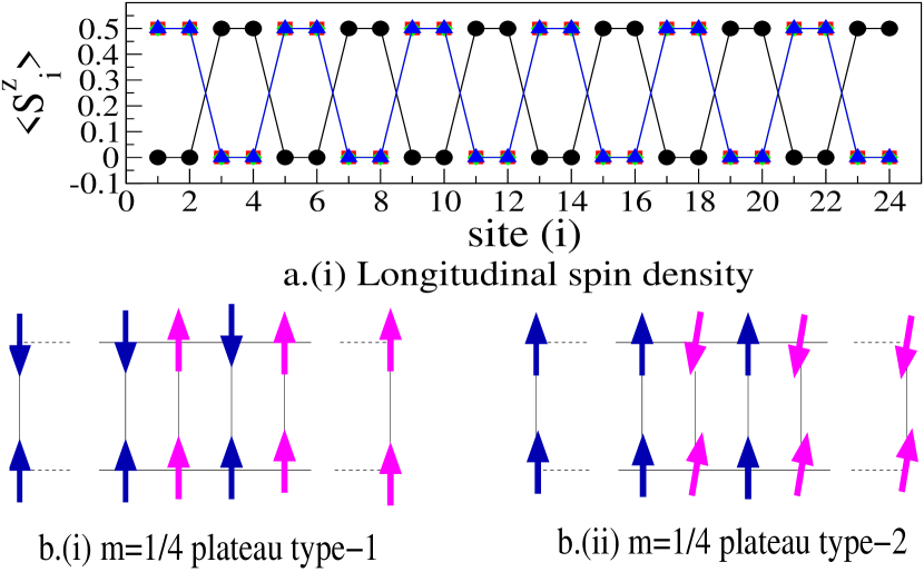
Figure 3: a.(i) Longitudinal spin density $S^{z}_{i}$ is shown as a function of site index $i$ for four GS phases: the SRFM ($J_{q}=0.2$,$J_{d}=2.0$), the AAFM ($J_{q}=2.0$,$J_{d}=0.4$), the Dimer ($J_{q}=2.0$,$J_{d}=1.0$), and the SLFM ($J_{q}=2.0$,$J_{d}=1.6$) using black, red, green, blue colors respectively. The spin configurations in b.(i) $m=1/4$ plateau type-1, b.(ii) $m=1/4$ plateau type-2 are shown. In $m=1/4$ plateau type-1, all the Heisenberg rung pairs $S-S$ (magenta spins) are fully polarized, and in $m=1/4$ plateau type-2, all the Ising rung pairs $\sigma-\sigma$ (blue spins) are fully polarized.

For a critical analysis of the $m=1/4$ plateau formation for all the phases, the spin density $\langle S^{z}_{i}\rangle$ is shown as a function of site index $i$ in Fig.3.a.(i). The SRFM phase is highly Ising dominated whereas, the other three phases are dominated by isotropic Heisenberg rung coupling. So, the mechanism of plateau formation is supposed to be different in all other phases than the SRFM phase. In the GS, the SRFM phase is highly frustrated with $J_{d}=2.0$ and $J_{q}=0.2$. The diagonal bond $J_{d}$ is more strong compared to others due to which it induces a finite gap between the non-magnetic ($S^{z}=0$) and magnetic ($S^{z}=N/4$) states. For the given set of parameters in this phase, a large field $h_{c1}=2.5$ is required to close the gap so that $m$ jumps from zero magnetization to $m=1/4$ plateau as shown in Fig.2.(i). For $h>2.5$, the weakly coupled Heisenberg type rung pairs $S-S$ have the finite value of spin density $0.5$ as shown in Fig.3.a.(i), which means that the $S-S$ pairs are aligned in the $m=1/4$ plateau phase. The spin configuration of this type of plateau is called $m=1/4$ plateau type-1 and it is shown in Fig.3.b.(i). The $m=1/4$ plateau phase also has a finite gap due to its stability coming from the strong $\sigma-\sigma$ rung pair for the large $J_{c}$, and it requires a field $h=3.5$ to close the gap to reach the saturation. The other three phases: the AAFM, the Dimer, and the SLFM have strong Heisenberg rung exchange ($J_{q}=2.0$), for which it forms strong singlets on the $S-S$ pairs, and are more stable energetically compared to the $\sigma-\sigma$ pairs with Ising type rung exchange. The AAFM phase has anisotropic antiferromagnetic spin alignment on the ladder with $J_{q}=2.0$, $J_{d}=0.4$, where, a very small field $h_{c1}=0.7$ is sufficient to break the $\sigma-\sigma$ pairs and to reach $m=1/4$ plateau as shown in Fig.2.(ii). In the $m=1/4$ plateau of AAFM, the rung spin pairs of $\sigma$ take the value $0.5$ of spin density as shown in Fig.3.a.(i). The spin configuration of this type of magnetic phase is called $m=1/4$ plateau type-2 and is shown in Fig.3.b.(ii). In the Dimer phase, all the Ising type exchanges are equal to unity for which it has a lesser spin gap than the AAFM phase, and it is closed by an external field $h_{c1}=0.5$ for the given $J_{q}(=2.0)$. Due to the perfect singlet formation of $S-S$ pairs through strong $J_{q}$ coupling in this case, the $m=1/4$ plateau has a much larger width than AAFM as shown in Fig.2.(iii). The GS of the SLFM phase has ferromagnetic spin arrangements along the leg, whereas, the legs are aligned oppositely to each other. Fig.2.(iv) shows that the $m=1/4$ plateau onsets at a field $h_{c1}=0.7$ and has the largest width. From the spin density, it is noticed that the Ising dimers are polarized along the field in the plateau phase. The Ising rungs are less energetic in this phase also like the AAFM, whereas, oppositely aligned legs enhance the stability of the singlets on the Heisenberg pair $S-S$, which gives rise to the largest plateau width. With further increase in field, the plateau is broken and a sharp jump takes place at $h_{c2}=4.5$. In all four phases, either all $S-S$ or all $\sigma-\sigma$ rung pairs are broken simultaneously, which results in magnetic jumps.

IV.1.2 Quantum Fidelity and Bipartite Concurrence

The plateau formation discussed above is quite different for the four phases, and it can be understood from the perspective of quantum information study also. In this subsection, we calculate and show the zero temperature limit quantum fidelity and bipartite concurrence to analyze the plateaus, and these can be obtained from the partition function as discussed below. Quantum fidelity is the measurement of overlap between two states and can be used to characterize the phase transition on the tuning of parameters. Quan et. al. have shown that for any field, fidelity can be obtained from the partition function Quan and Cucchietti (2009). Similarly, we calculate the quantum fidelity for the field $h$ with small perturbation $\delta h$ as: $\mathcal{F}(h,\beta)=\frac{Q_{4}(h,\beta)}{\sqrt{Q_{4}(h+\delta h,\beta)Q_{4}(h-\delta h,\beta)}}$, where $Q_{4}(h,\beta)$ is the partition function for one unit cell in our case Eq.2. Field fidelity susceptibility can also be obtained as $\mathcal{\chi}(h,\beta)=\frac{\partial\mathcal{F}(h,\beta)}{\partial h}$. $\mathcal{F}(h,\beta)$ is unity when there is a unique state and discontinuous at the phase transition points. Fig.4.a.[(i)-(iv)], and b.[(i)-(iv)] show the plot of $\mathcal{F}(h,\beta)$ (left column) and $\mathcal{\chi}(h,\beta)$ (right column) as a function of $h$ respectively for four different phases: (i) the SRFM, (ii) the AAFM, (iii) the Dimer, and (iv) the SLFM. In each of the sub-figures of $\mathcal{F}(h,\beta)$ and $\mathcal{\chi}(h,\beta)$, two discontinuities are noticed for all four phases. All of these discontinuities are consistent with the jumps of the $m-h$ curve in Fig.2 and represent the magnetic phase transitions.

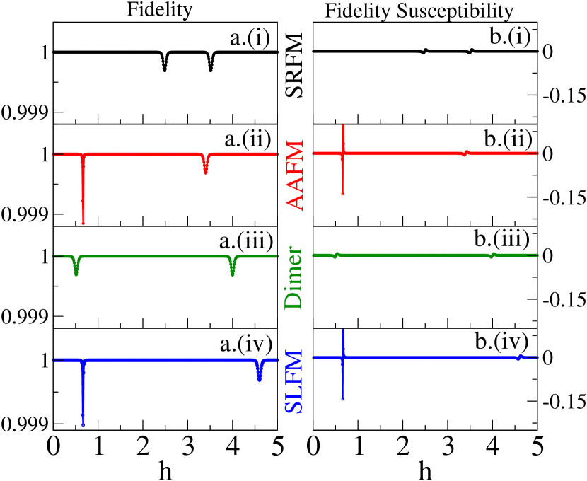
Figure 4: (a) (left column) Quantum fidelity and (b) (right column) fidelity susceptibility calculated using TM are shown for the thermodynamic limit ($N\rightarrow\infty$) at $T/J_{c}\rightarrow 0$. Black, red, green, and blue colors representing four phases: the SRFM ($J_{q}=0.2$,$J_{d}=2.0$), the AAFM ($J_{q}=2.0$,$J_{d}=0.4$), the Dimer ($J_{q}=2.0$,$J_{d}=1.0$), and the SLFM ($J_{q}=2.0$,$J_{d}=1.6$) respectively are arranged sequentially from top to bottom in both the columns.

We also calculate the bond order to understand the configurational change and bipartite concurrence to measure the quantum nature of the $S-S$ pair which is connected through a Heisenberg rung exchange $J_{q}$. If the concurrence has some finite value, the wavefunction is in a mixed or entangled state, otherwise, it is in a pure state if the concurrence is zero. Wooters et.al. and Karlova et. al. in their study calculate concurrence for a spin pair connected by Heisenberg interaction in terms of the local pair magnetization and spatial correlations: longitudinal, transverse to detect phase transitions at a finite temperature Wootters (1998); Karľová and Strecka (2020). In our study, we calculate the bipartite concurrence for the Heisenberg rung pair connected by $J_{q}$ as

$$\mathcal{C}(J_{q},h)=max\Big{\{}0,4|{c^{T}(J_{q},h)}|-$$

$$2\sqrt{(\frac{1}{4}+(c^{L}(J_{q},h))^{2}-m^{2}(J_{q},h)}\Big{\}}$$ (7)

Where, $m(J_{q},h)$, $c^{L}(J_{q},h)$ and $c^{L}(J_{q},h)$ are the pair magnetization, the longitudinal and transverse component of bond order respectively, and these can be defined as:
$m(J_{q},h)=\frac{m(h,\beta)}{2}=-\frac{1}{2}\frac{\partial{F(h,T)}}{\partial{h}}$
$c^{L}(J_{q},h)=\big{<}S^{z}_{2i,1}S^{z}_{2i,2}\big{>}=-\frac{1}{4\beta}\frac{\partial{[\log{Q_{4}(h,T)}]}}{\partial{J_{q}}}$
$c^{T}(J_{q},h)=\big{<}S^{x}_{2i,1}S^{x}_{2i,2}\big{>}=-\frac{1}{8\beta}\frac{\partial{[\log{Q_{4}(h,T)}]}}{\partial{J_{q}}}$

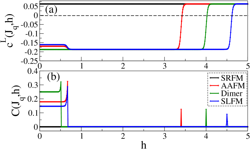
Figure 5: (a) Longitudinal bond order $c^{L}(J_{q},h)$, (b) Quantum concurrence $\mathcal{C}(J_{q},h)$ for the Heisenberg spin pair $S-S$ connected by rung strength $J_{q}$ are shown as a function $h$. Black, red, green, and blue colors represent four phases: the SRFM ($J_{q}=0.2$,$J_{d}=2.0$), the AAFM ($J_{q}=2.0$,$J_{d}=0.4$), the Dimer ($J_{q}=2.0$,$J_{d}=1.0$), and the SLFM ($J_{q}=2.0$,$J_{d}=1.6$) respectively at $T/{J_{c}}=0.02$.

The longitudinal bond order $c^{L}(J_{q},h)$ is shown in Fig.5.(a) for all the four phases (i) the SRFM, (ii) the AAFM, (iii) the Dimer, and (iv) the SLFM. In the SRFM phase, the small positive value of $c^{L}(J_{q},h)$ indicates the ferromagnetic alignment of $S-S$ pair for any value of $h$. Because, $c^{L}(J_{q},h)$ and $c^{T}(J_{q},h)$ both are small, the Eq.7 demands the $\mathcal{C}(J_{q},h)$ to be always zero, which in other words can be thought of as there is no quantum concurrence or no quantum entanglement between the two $S$ spins. For the other three cases: the AAFM, the Dimer, and the SLFM, $c^{L}(J_{q},h)$ is negative below a critical field $h_{c2}$, and then it goes to a positive value for $h>h_{c2}$. Above the certain field $h_{c1}$ and below $h_{c2}$, the system is in the $m=1/4$ plateau as it is noticed in Fig.5.(a) and (b), which is consistent with the magnetic jumps in Fig.2.[(i)-(iv)]. Since, the Heisenberg rung pair spins $S-S$ are still anti-parallel for $h_{c1}<h<h_{c2}$, $c^{L}(J_{q},h)$ also supports the $m=1/4$ plateau type-2 configuration as shown in Fig.3.b.(ii). The concurrence $\mathcal{C}(J_{q},h)$ is positive i.e, entangled below $h_{c1}$ for the AAFM, the Dimer, and the SLFM phases. However, for $h>h_{c2}$ because both the bond orders: longitudinal and transverse are very small positives, the Eq.7 takes the value of $\mathcal{C}_{J_{q}}$ to zero and the spin pairs $S-S$ loose quantum concurrence in the saturation magnetization and becomes a pure state.

IV.2 Magnetization process in the presence of a transverse field

Using many experimental techniques in general, this kind of system is synthesized in powder form or single crystal form and so to understand the directional dependence of the field on the magnetization, we study the effect of the transverse field $h^{x}$ in our model Guo et al. (2020); Kakarla et al. (2021). In presence of $h^{x}$, the Hamiltonian of different units do not commute to each other, and therefore, the TM method never works, we use the ED method to show the finite size scaling of magnetization for three system sizes and then analyze the spin density for $N=24$.

IV.2.1 Transverse component of magnetization

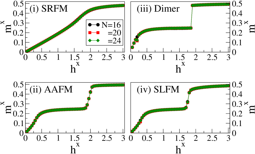
Figure 6: Transverse magnetization $m^{x}$ is shown as a function of the transverse field $h^{x}$ for four phases: (i) SRFM ($J_{q}=0.2$, $J_{d}=2.0$), (ii) AAFM ($J_{q}=2.0$, $J_{d}=0.4$) (iii) Dimer ($J_{q}=2.0$, $J_{d}=1.0$), and (iv) SLFM ($J_{q}=2.0$, $J_{d}=1.6$). Black, red, and green colors represent the system sizes $N=16,20,\text{and}~{}24$ respectively.

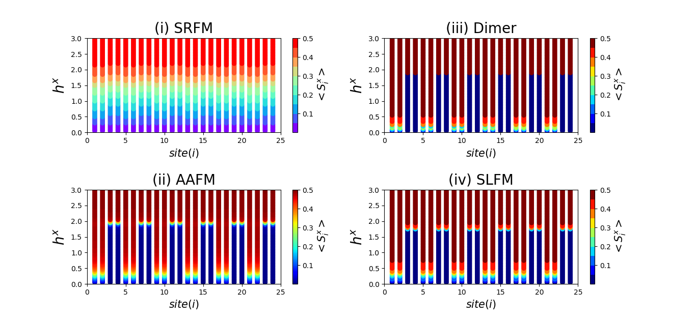
Figure 7: Transverse component of spin density $\langle S^{x}_{i}\rangle$ at each site $i$ for for four phases: (i) SRFM ($J_{q}=0.2$, $J_{d}=2.0$), (ii) AAFM ($J_{q}=2.0$, $J_{d}=0.4$) (iii) Dimer ($J_{q}=2.0$, $J_{d}=1.0$), and (iv) SLFM ($J_{q}=2.0$, $J_{d}=1.6$) are shown for system size $N=24$. Along the horizontal axis, the site index $i$ for each spin is shown. Along the vertical axis, the transverse field $h^{x}$ is varied. The color bar shown in all subfigures represents the amplitude of $\langle S^{x}_{i}\rangle$ and it varies from $0$ to $0.5$ for spin-1/2 systems.

It is to be mentioned that all four GS phases are in the $S^{z}=0$ sector, and so it does not change the longitudinal but rather the transverse component of magnetization on the application of an external transverse field $h^{x}$. We calculate the transverse magnetization $m^{x}$ in terms of spin density $\langle S^{x}_{i}\rangle$ at each site $i$ as-

$$m^{x}=\frac{1}{N}\sum_{i=1}^{N}\langle S_{i}^{x}\rangle$$ (8)

In Fig.6[(i)-(iv)], we show the transverse (along $+x$ direction) magnetization for all four phases: (i) the SRFM, (ii) the AAFM, (iii) the Dimer, and (iv) the SLFM with the corresponding set of chosen $J_{q}$, $J_{d}$ values as in section IV.1.1 for the system sizes $N=16,20$, and $24$. In the SRFM phase, the $m^{x}$ shows continuous variation with the field $h^{x}$ up to saturation value. In this phase, the GS has Ising bond dominance for all the spins, and therefore the spins along the x-direction get smoothly oriented along the field. In the AAFM phase, the curve increases smoothly and then it shows a $m^{x}\approx 1/4$ plateau-like behavior in the range $0.45<h^{x}<1.75$, and afterward it jumps to full saturation. A similar behavior is noticed in the Dimer phase as well in which the plateau onsets at a field $h^{x}=0.4$. In this case, the jump from the $m^{x}=1/4$ plateau to saturation is much faster than in the case of the AAFM phase. In the SLFM phase for $h^{x}<0.7$, $m^{x}$ increases smoothly, and then it forms the plateau-like structure for $0.7<h^{x}<1.7$. It shows a sudden jump almost around $h^{x}=1.75$ and slowly reaches saturation magnetization for higher $h^{x}$. From all the subfigures, it is noticed that there is a negligibly small finite-size effect. In the next subsection, we analyze the $m^{x}=1/4$ plateau mechanism for all the phases based on the spin density.

IV.2.2 Transverse component of spin density

For a more detailed understanding, we show the color map of the spin density $\langle S^{x}_{i}\rangle$ in all four phases for $N=24$. It is to be mentioned that the $\sigma-\sigma$ and $S-S$ pairs alternate with site index $i$. To be more specific, $\sigma-\sigma$ pairs take the site indices [1,2,5,6,….] whereas, $S-S$ pairs take the indices [3,4,7,8….] as shown in all subfigures of Fig.7. In Fig.7.(i), $\langle S^{x}_{i}\rangle$ varies continuously as $h^{x}$ increases for all the sites. As the GS of the SRFM has only Ising interactions dominance and there is no transverse spin correlation, all the spins continuously get oriented along $h^{x}$ in this phase. In the AAFM phase, the $S-S$ pair has a strong transverse spin correlation whereas, the $\sigma-\sigma$ rung pairs are weak and are aligned continuously with an increase in $h^{x}$ as shown in the color map Fig.7.(ii). Saturation is attained by an even further increase of field when it breaks the strong $S-S$ pair at $h^{x}=1.75$. As shown in Fig.7.(iii) for the Dimer phase, the continuous increase of $m^{x}$ is similar to the AAFM phase but a sudden jump at $h^{x}=1.7$ is noticed because of unbinding of the perfect $S-S$ singlet pairs. Fig.7.(iv) shows $\langle S^{x}_{i}\rangle$ for the SLFM phase. As in the GS of this phase, both the Ising pairs and Heisenberg pairs are aligned parallel but spins of opposite legs are aligned oppositely, with the increase in $h^{x}$, it is noticed that all the Ising dimer pairs are continuously broken until the magnetization reaches to $1/4$. An even further increase in $h^{x}$ does not easily close the spin gap and results in a large $m^{x}=1/4$ plateau until a field $h^{x}=1.75$ is applied to break the Heisenberg rung $S-S$ pairs.

V Summary

In this manuscript, we study the effect of external magnetic field on the GS phases of Hamiltonian in Eq.II of a frustrated spin-$\frac{1}{2}$ two-leg ladder with alternate Ising and Heisenberg type of rung and Ising type of interaction in the leg and diagonal. Tuning of the exchange parameters in the model Hamiltonian can give rise to four GS phases: (i) the SRFM, (ii) the AAFM, (iii) the Dimer, and (iv)the SLFM, whose spin arrangements are schematically represented in Fig.1.b. [(i)-(iv)]. We analyzed the magnetization behavior in the presence of external magnetic fields: longitudinal and transverse. In the presence of the longitudinal magnetic field $h$, the GS shows three magnetic plateaus: the first one is due to the finite spin gap, the second plateau at $m=1/4$ is formed due to the polarization of either type of rung spin dimers along the field. This can be of two types as shown in Fig.3.b. In the SRFM phase, the Heisenberg rung spin pairs $S-S$ are polarized giving rise to $m=1/4$ plateau type-1 as shown in Fig.3.b.(i). But for the other three phases: the AAFM, the Dimer, and the SLFM, the $\sigma-\sigma$ spins are polarized at $m=1/4$ and give rise to plateau type-2 as shown in Fig.3.b.(ii). In the presence of a large external field in all phases, all of the spins are completely polarized along the field and form the third plateau at the saturation magnetization $m=1/2$. The $m=1/4$ plateau width is sensitive to the parameter values as obtained in Eq.6. We also notice that two plateaus are connected by jumps in the magnetization curve and this is because of the unpairing of either all $S-S$ or all $\sigma-\sigma$ rung dimers.

To understand the quantum nature of the wave function of the GS, we calculate the quantum fidelity and quantum concurrence in the presence of a longitudinal field. In all four phases, fidelity shows deviation from unity at the critical fields of magnetic phase transitions as shown in Fig.4. The quantum concurrence shown in Fig.5 measures the entanglement between two spins at the Heisenberg rung. The concurrence is always zero as a function of the field for the SRFM phase, and it means that the SRFM phase is a pure state. Whereas, in other phases: the AAFM, the Dimer, and the SLFM, the concurrence has a finite value below a critical field before the formation of the $m=1/4$ plateau. In these phases, the zero plateau is a mixed or entangled state but the other two plateaus are pure states. However, all of the jumps in the magnetization can be indirectly predicted based on the jumps in concurrence also as shown in Fig.5.

In the SRFM phase, spin alignments are along the z direction and there is weak exchange interaction along the +x direction in the Heisenberg rung dimers, therefore, magnetization $m^{x}$ shows a continuous variation till saturation on the application of a transverse field. In other phases: the AAFM, the Dimer, and the SLFM, the magnetization process can be understood in terms of two sublattice behavior. The sublattice with $\sigma-\sigma$ dimer is paramagnetic along x, whereas, in the other sublattice, the Heisenberg spin pair $S-S$ dimer has a strong transverse exchange component which induces a finite spin gap in the system. As a consequence, at a lower value of the transverse field, the system shows a continuous behavior in the magnetization curve due to gradual change of $m^{x}$ of $\sigma-\sigma$ spins upto $m^{x}=1/4$ with an increase in $h^{x}$ as shown using spin density in Fig.7.[(ii)-(iv)]. With further increase in field, at a critical value, the magnetization curve shows a sudden jump from $m^{x}\approx 1/4$ to $1/2$ for the three phases: the AAFM, the Dimer, and the SLFM, and this phase transition seems to be of the first order. The plateau width is sensitive to the set of parameters or the set of exchange interactions $J_{q}$ and $J_{d}$ in the presence of a transverse field also. In conclusion, this model system gives many insightful mechanisms of the plateau and jumps and these magnetic properties can be utilized in designing quantum switches, magnetic memories, and other similar devices. Also, these systems might have tremendous applications in quantum information processing and quantum computation.

VI Acknowledgements

M.K. thanks SERB Grant Sanction No. CRG/2022/000754 for the computational facility. S.S.R. thanks CSIR-UGC for financial support.

VII Appendix

The partition function in presence of a longitudinal field $h$ for $N$ sites, $Q_{N}(h,\beta)$ with Hamiltonian $H$ can be written as-

$$Q_{N}(h,\beta)=Tr\left(e^{-\beta\textbf{H}}\right)$$ (9)

where, Tr means trace of the matrix, $\beta=1/\left(k_{B}T\right)$ and $k_{B}$ is the Boltzmann constant. Using explicit configuration basis for the system, Eq. 9 is rewritten in the following form,

$$Q_{N}(h,\beta)=\sum_{\{\sigma,S\}}<\cdots,\sigma_{2i-1,1},\sigma_{2i-1,2},S_{2i,1},S_{2i,2},\cdots\mid e^{-\beta\mathbf{H}}\mid\cdots,\sigma_{2i-1,1},\sigma_{2i-1,2},S_{2i,1},S_{2i,2},\cdots>,$$

here the summation is over all possible configurations $\{\sigma,S\}$ of the system. For a given configuration, $|\cdots,\sigma_{2i-1,1},\sigma_{2i-1,2},S_{2i,1},S_{2i,2},\cdots>$ represents a basis state. In our case, the system is composed of $n=N/4$ units, and for each unit, the Hamiltonian is written in Eq.II. The partition function of the entire ladder can be written as:

$$Q_{N}(h,\beta)=\sum_{\sigma}<\cdots,\sigma_{2i-1,1},\sigma_{2i-1,2},\cdots\mid\prod_{i=1}^{n}\mathbf{T}_{i}\mid\cdots,\sigma_{2i-1,1},\sigma_{2i-1,2},\cdots>$$

where $T_{i}=\sum_{\{S\}_{i}}<S_{2i,1},S_{2i,2}\mid e^{-\beta\mathbf{H_{i}}(\sigma,S)}\mid S_{2i,1},S_{2i,2}>$ is well-known transfer matrix operator for each unit. Here the summation is over $\{S\}_{i}$ which represents all possible configurations of spins $S_{2i,1}$ and $S_{2i,2}$ (from the $i^{th}$ unit). It may be noted that $T_{i}$ does not contain the components of spin $S$ operators and it has only $\sigma$ variables, namely, $\sigma_{2i-1,1},\sigma_{2i-1,2},\sigma_{2i+1,1}$ and $\sigma_{2i+1,2}$. Since, the Hamiltonians of each unit commute to each other, by introducing identity operators $I=\sum_{\{\sigma\}_{i}}|\sigma_{2i-1,1},\sigma_{2i-1,2}><\sigma_{2i-1,1},\sigma_{2i-1,2}|$ between successive $\mathbf{T}$ operators, we can finally write the partition function as the trace of the $n$-th power of a small ($4\times 4$) transfer matrix $\mathbf{P}$. We have,

$$Q_{N}(h,\beta)=Tr(\mathbf{P}^{n}),$$

The elements of the transfer matrix are given by

$$P_{(\sigma_{2i-1,1},\sigma_{2i-1,2}),(\sigma_{2i+1,1},\sigma_{2i+1,2})}=<\sigma_{2i-1,1},\sigma_{2i-1,2}\mid\mathbf{T}_{i}\mid\sigma_{2i+1,1},\sigma_{2i+1,2}>$$ (10)

Before we construct and diagonalize the $\mathbf{P}$ matrix, we first need to carry out the trace over the configurations $\{S\}_{i}$ to find out the form of $\mathbf{T}_{i}$. Since $\mathbf{T}_{i}=\sum_{\{S\}_{i}}<S_{2i,1},S_{2i,2}\mid e^{-\beta\mathbf{H_{i}}(\sigma,S)}\mid S_{2i,1},S_{2i,2}>$, if we take the eigenstate basis of $\mathbf{H}_{i}$, we will get $\mathbf{T}_{i}$ as the summation over exponential of eigenvalues of $-\beta\mathbf{H}_{i}$. Next, we calculate the eigenvalues of $\mathbf{H}_{i}$ operator.

By considering,
$a=J_{d}\left(\sigma_{2i-1,2}^{z}+\sigma_{2i+1,2}^{z}\right)+J_{cq}\left(\sigma_{2i-1,1}^{z}+\sigma_{2i+1,1}^{z}\right)$
+$h$
$b=J_{d}\left(\sigma_{2i-1,1}^{z}+\sigma_{2i+1,1}^{z}\right)+J_{cq}\left(\sigma_{2i-1,2}^{z}+\sigma_{2i+1,2}^{z}\right)$
+$h$
$c=\frac{J_{c}}{2}\left(\sigma_{2i-1,1}^{z}\sigma_{2i-1,2}^{z}+\sigma_{2i+1,1}^{z}\sigma_{2i+1,2}^{z}\right)$
$d=\frac{h}{2}\left(\sigma_{2i-1,1}^{z}+\sigma_{2i-1,2}^{z}+\sigma_{2i+1,1}^{z}+\sigma_{2i+1,2}^{z}\right)$,
$f=c+d$
Hamiltonian (Eq. II ) for the $i^{th}$ geometrical unit can be written as-

$$\mathbf{H_{i}}=\frac{J_{q}}{2}\left(S_{2i,1}^{+}S_{2i,2}^{-}+S_{2i,1}^{-}S_{2i,2}^{+}\right)+J_{q}\left(S_{2i,1}^{z}S_{2i,2}^{z}\right)+aS_{2i,1}^{z}+bS_{2i,2}^{z}+f$$

We can write down the following Hamiltonian matrix in the eigenstate basis of $S_{2i,1}^{z}S_{2i,2}^{z}$ operator,

$$H_{i}=\left[\begin{array}[]{cccc}\frac{J_{q}}{4}+\frac{(a+b)}{2}+f&0&0&0\\ 0&\frac{-J_{q}}{4}+\frac{(a-b)}{2}+f&\frac{J_{q}}{2}&0\\ 0&\frac{J_{q}}{2}&\frac{-J_{q}}{4}-\frac{(a-b)}{2}+f&0\\ 0&0&0&\frac{J_{q}}{4}-\frac{(a+b)}{2}+f\\ \end{array}\right].$$

The Hamiltonian matrix comes up with its four eigenvalues from three $S^{z}_{SS}$ sectors based on S-S pairs-
(i) From $S^{z}_{SS}=1$ sector (formed by S-S pair)
$\theta_{1}=(f+\frac{J_{q}}{4})+\frac{(a+b)}{2}$
(ii) From $S^{z}_{SS}=-1$ sector (formed by S-S pair)
$\theta_{2}=(f+\frac{J_{q}}{4})-\frac{(a+b)}{2}$
(iii) From $S^{z}_{SS}=0$ sector (formed by S-S pair)
$\theta_{3}=(f-\frac{J_{q}}{4})+\frac{\sqrt{J_{q}^{2}+(a-b)^{2}}}{2}$
$\theta_{4}=(f-\frac{J_{q}}{4})-\frac{\sqrt{J_{q}^{2}+(a-b)^{2}}}{2}$.

We note that the eigenvalues ($\theta_{k}$) are functions of $\sigma$ variables, namely $\sigma_{2i-1,1},\sigma_{2i-1,2},\sigma_{2i+1,1}$ and $\sigma_{2i+1,2}$. Using these eigenvalues, we rewrite $\mathbf{T}_{i}$ as,

$$\mathbf{T}_{i}=\sum_{\{S\}_{i}}<S_{2i,1},S_{2i,2}\mid e^{-\beta\mathbf{H_{i}}(\sigma,S)}\mid S_{2i,1},S_{2i,2}>$$

$$~{}~{}~{}=\sum_{k=1}^{4}e^{-\beta\theta_{k}}.$$

$$=2e^{-\beta f}\bigg{[}e^{-\frac{\beta J_{q}}{4}}cosh\bigg{(}\frac{\beta(a+b)}{2}\bigg{)}$$

$$+e^{\frac{\beta J_{q}}{4}}cosh\bigg{(}\frac{\beta J_{q}}{2}\sqrt{1+\frac{(a-b)^{2}}{J_{q}^{2}}}\bigg{)}\bigg{]}$$

Further, we consider- $e^{\frac{\beta J_{q}}{4}}=Q$ , $e^{\frac{\beta J_{c}}{4}}=C$
$e^{\frac{\beta h}{4}}=H$ , $\frac{(J_{cq}+J_{d})}{2}=X$ $\frac{(J_{cq}-J_{d})^{2}}{J^{2}_{q}}=Y$
and also, $\Delta_{1}=\sqrt{1+Y}$, $\Delta_{2}=\sqrt{1+4Y}$

The Transfer matrix for one unit becomes -

$$\mathbf{P}=\left[\begin{array}[]{cccc}p&q&q&r\\ q&s&u&v\\ q&u&s&v\\ r&v&v&w\\ \end{array}\right].$$

Where,

$$p=2e^{-\beta(J_{c}/4+h)}$$

$$\times\bigg{[}Q^{-1}cosh\big{(}\beta(2X+h)\big{)}+Qcosh\big{(}\beta\frac{J_{q}}{2}\big{)}\bigg{]}$$

$$q=2e^{-\beta(h/2)}$$

$$\times\bigg{[}Q^{-1}cosh\big{(}\beta(X+h)\big{)}+Qcosh\big{(}\beta\frac{J_{q}\Delta_{1}}{2}\big{)}\bigg{]}$$

$$r=2e^{-\beta(J_{c}/4)}$$

$$\times\bigg{[}Q^{-1}cosh\big{(}\beta h\big{)}+Qcosh\big{(}\beta\frac{J_{q}}{2}\big{)}\bigg{]}$$

$$s=2e^{\beta(J_{c}/4)}$$

$$\times\bigg{[}Q^{-1}cosh\big{(}\beta h\big{)}+Qcosh\big{(}\beta\frac{J_{q}\Delta_{2}}{2}\big{)}\bigg{]}$$

$$u=2e^{\beta(J_{c}/4)}$$

$$\times\bigg{[}Q^{-1}cosh\big{(}\beta h\big{)}+Qcosh\big{(}\beta\frac{J_{q}}{2}\big{)}\bigg{]}$$

$$v=2e^{\beta(h/2)}$$

$$\times\bigg{[}Q^{-1}cosh\big{(}\beta(-X+h)\big{)}+Qcosh\big{(}\beta\frac{J_{q}\Delta_{1}}{2}\big{)}\bigg{]}$$

$$w=2e^{-\beta(J_{c}/4-h)}$$

$$\times\bigg{[}Q^{-1}cosh\big{(}\beta(-2X+h)\big{)}+Qcosh\big{(}\beta\frac{J_{q}}{2}\big{)}\bigg{]}$$

From $|P-\lambda I_{4}|=0$, we get the eigenvalues in the form of

$$\framebox{$\lambda_{4}=(s-u)$}$$

$$\framebox{$\lambda^{3}-B_{0}\lambda^{2}-C_{0}\lambda+D_{0}=0$}$$ (11)

Here, $\lambda_{4}$ is one of the eigenvalues, whereas, the other three come from Eq.VII. The coefficients of the equation are defined as:

$$B_{0}=(s+u+w)$$

$$C_{0}=[2(q^{2}+v^{2}-\frac{r^{2}}{2})-pw+(p-w)(s+u)]$$

$$D_{0}=[4qrv-2pv^{2}-2q^{2}w+pw^{2}-(s+u)(r^{2}+pw)]$$

For the polynomial equation VII, the eigenvalues $\lambda_{i}$ satisfy the relations-

$$\sum^{3}_{i=1}\lambda_{i}=B_{0},\sum^{3}_{i=1}\lambda_{i}\lambda_{i+1}=-C_{0}$$ (12)

Now, let us make a very reasonable assumption to make the calculation easy. We assume, $\lambda_{1}\gg\lambda_{2}\gg\lambda_{3}$ are in descending order and $\lambda_{3}$ has the least contribution in the partition function so that Eq.12 can approximately be written as:

$$\lambda_{1}+\lambda_{2}=B_{0},\lambda_{1}\lambda_{2}=-C_{0}$$ (13)

The Eq. 13 leads us to getting other two eigenvalues:

$$\lambda^{2}_{1,2}-B_{0}\lambda_{1,2}-C_{0}=0$$

$$\framebox{$\Longrightarrow\lambda_{1,2}=\frac{B_{0}\pm\sqrt{B^{2}_{0}+4C_{0}}}{2}$}$$ (14)

We find Eq. VII becomes much more simpler with further approximation in $\beta\rightarrow\infty$ limit as-

$$\lambda_{1}=(w+s+u)$$

$$=2e^{\frac{-\beta(J_{c}-4h)}{4}}$$

$$\times\bigg{[}Q^{-1}cosh[\beta(h-2X)]+Qcosh[\frac{\beta J_{q}}{2}]\bigg{]}$$

$$+2e^{\frac{\beta J_{c}}{4}}$$

$$\times\bigg{[}2Q^{-1}cosh[\beta h]+Qcosh[\frac{\beta J_{q}\Delta_{2}}{2}]+Qcosh[\frac{\beta J_{q}}{2}]\bigg{]}$$

$Q_{N}(h,\beta)$ takes the form as
$Q_{N}(h,\beta)=[\lambda_{1}+\lambda_{2}+\lambda_{3}+\lambda_{4}]^{n}$
For $n\rightarrow\infty$, and $\lambda_{1}$ being the largest, the partition function for the entire system and one unit become $Q_{N}(h,\beta)\approx[\lambda_{1}]^{n}$ and $Q_{4}(h,\beta)\approx\lambda_{1}$ respectively.

Now, we write down $\lambda_{1}$ as a polynomial function of $e^{\beta h}$ as

$$\lambda_{1}=a_{0}e^{2\beta h}+b_{0}e^{\beta h}+c_{0}e^{-\beta h}+d_{0}$$ (16)

We define the system parameters as follows-
$a_{0}=e^{-\frac{\beta}{4}(J_{q}+J_{d}+2)}$,
$b_{0}=2e^{-\frac{\beta}{4}(J_{q}-1)}+2e^{\frac{\beta}{4}(J_{q}-1)}Cosh[\frac{\beta J_{q}}{2}]$,
$c_{0}=2e^{-\frac{\beta}{4}(J_{q}-1)}$,
$d_{0}=2Cosh[\frac{\beta J_{q}}{2}](e^{\frac{\beta J_{q}}{4}}+e^{\frac{-\beta}{4}})+2e^{\frac{\beta J_{q}}{4}}Cosh[\frac{\beta J_{q}\Delta_{2}}{2}]+e^{\frac{\beta(7+8J_{d}+J_{q})}{4}}$
By equating the differential of the free energy with respect to magnetization to zero i.e, $\frac{\partial{F}}{\partial{m}}=0$, two critical fields $h_{\pm}$ are obtained as

$$h_{\pm}=\frac{1}{\beta}ln\big{[}\frac{b_{0}\pm\sqrt{b^{2}_{0}-3a_{0}d_{0}}}{3a_{0}}\big{]}$$ (17)

References

- Nakamura and Okamoto (1998) T. Nakamura and K. Okamoto, Physical Review B 58, 2411 (1998).
- Guo et al. (2020) S. Guo, R. Zhong, K. Górnicka, T. Klimczuk, and R. J. Cava, Chemistry of Materials 32, 10670 (2020).
- Kakarla et al. (2021) D. C. Kakarla, Z. Yang, H. Wu, T. Kuo, A. Tiwari, W.-H. Li, C. Lee, Y.-Y. Wang, J.-Y. Lin, C. Chang, et al., Materials Advances 2, 7939 (2021).
- Dagotto and Rice (1996) E. Dagotto and T. M. Rice, Science 271, 618 (1996).
- Chubukov (1991) A. V. Chubukov, Phys. Rev. B 44, 4693 (1991).
- Chubukov et al. (1994) A. V. Chubukov, S. Sachdev, and J. Ye, Physical Review B 49, 11919 (1994).
- Hutchings M T (1979) M. J. M. Hutchings M T, Ikeda H, Journal of Physics C, Solid State Physics 18, L739 (1979).
- Park et al. (2007) S. Park, Y. J. Choi, C. L. Zhang, and S.-W. Cheong, Phys. Rev. Lett. 98, 057601 (2007).
- Mourigal et al. (2012) M. Mourigal, M. Enderle, B. Fåk, R. K. Kremer, J. M. Law, A. Schneidewind, A. Hiess, and A. Prokofiev, Phys. Rev. Lett. 109, 027203 (2012).
- Drechsler et al. (2007) S.-L. Drechsler, O. Volkova, A. N. Vasiliev, N. Tristan, J. Richter, M. Schmitt, H. Rosner, J. Málek, R. Klingeler, A. A. Zvyagin, and B. Büchner, Phys. Rev. Lett. 98, 077202 (2007).
- Dutton et al. (2012a) S. E. Dutton, M. Kumar, Z. G. Soos, C. L. Broholm, and R. J. Cava, Journal of Physics: Condensed Matter 24, 166001 (2012a).
- Dutton et al. (2012b) S. E. Dutton, M. Kumar, M. Mourigal, Z. G. Soos, J.-J. Wen, C. L. Broholm, N. H. Andersen, Q. Huang, M. Zbiri, R. Toft-Petersen, and R. J. Cava, Phys. Rev. Lett. 108, 187206 (2012b).
- Maeshima et al. (2003) N. Maeshima, M. Hagiwara, Y. Narumi, K. Kindo, T. C. Kobayashi, and K. Okunishi, Journal of Physics: Condensed Matter 15, 3607 (2003).
- Sandvik et al. (1996) A. W. Sandvik, E. Dagotto, and D. J. Scalapino, Phys. Rev. B 53, R2934 (1996).
- Johnston et al. (1987) D. C. Johnston, J. W. Johnson, D. P. Goshorn, and A. J. Jacobson, Phys. Rev. B 35, 219 (1987).
- Vekua et al. (2003) T. Vekua, G. Japaridze, and H.-J. Mikeska, Physical Review B 67, 064419 (2003).
- Richter et al. (2004) J. Richter, J. Schulenberg, and A. Honecher, “Quantum magnetism in two dimensions: From semi-classical néel order to magnetic disorder in quantum magnetism, ed. u. schollwöck, j. richter, djj farnell and rf bishop,” (2004).
- Ogino et al. (2021) T. Ogino, R. Kaneko, S. Morita, S. Furukawa, and N. Kawashima, Physical Review B 103, 085117 (2021).
- Ogino et al. (2022) T. Ogino, R. Kaneko, S. Morita, and S. Furukawa, Physical Review B 106, 155106 (2022).
- Luttinger (1963) J. Luttinger, Journal of mathematical physics 4, 1154 (1963).
- Sakai et al. (2022) T. Sakai, R. Nakanishi, T. Yamada, R. Furuchi, H. Nakano, H. Kaneyasu, K. Okamoto, and T. Tonegawa, Physical Review B 106, 064433 (2022).
- Maiti and Kumar (2019) D. Maiti and M. Kumar, Phys. Rev. B 100, 245118 (2019).
- Balents (2010) L. Balents, Nature 464, 199 (2010).
- Liao et al. (2017) H.-J. Liao, Z.-Y. Xie, J. Chen, Z.-Y. Liu, H.-D. Xie, R.-Z. Huang, B. Normand, and T. Xiang, Physical review letters 118, 137202 (2017).
- Barnes et al. (1993) T. Barnes, E. Dagotto, J. Riera, and E. Swanson, Physical Review B 47, 3196 (1993).
- Johnston et al. (2011) D. Johnston, R. McQueeney, B. Lake, A. Honecker, M. Zhitomirsky, R. Nath, Y. Furukawa, V. Antropov, and Y. Singh, Physical Review B 84, 094445 (2011).
- Kumar et al. (2015) M. Kumar, A. Parvej, and Z. G. Soos, Journal of Physics: Condensed Matter 27, 316001 (2015).
- Chitra et al. (1995) R. Chitra, S. Pati, H. R. Krishnamurthy, D. Sen, and S. Ramasesha, Phys. Rev. B 52, 6581 (1995).
- White and Affleck (1996) S. R. White and I. Affleck, Phys. Rev. B 54, 9862 (1996).
- Rahaman et al. (2023) S. S. Rahaman, S. Haldar, and M. Kumar, Journal of Physics: Condensed Matter (2023).
- Rakov et al. (2016) M. V. Rakov, M. Weyrauch, and B. Braiorr-Orrs, Phys. Rev. B 93, 054417 (2016).
- Mikeska and Kolezhuk (2004) H.-J. Mikeska and A. K. Kolezhuk, Quantum magnetism , 1 (2004).
- Wessel et al. (2017) S. Wessel, B. Normand, F. Mila, and A. Honecker, SciPost Physics 3, 005 (2017).
- Morita et al. (2015) S. Morita, R. Kaneko, and M. Imada, Journal of the Physical Society of Japan 84, 024720 (2015).
- Hijii et al. (2005) K. Hijii, A. Kitazawa, and K. Nomura, Physical Review B 72, 014449 (2005).
- Agrapidis et al. (2019) C. E. Agrapidis, J. van den Brink, and S. Nishimoto, Phys. Rev. B 99, 224418 (2019).
- Liu et al. (2022) W.-Y. Liu, S.-S. Gong, Y.-B. Li, D. Poilblanc, W.-Q. Chen, and Z.-C. Gu, Science bulletin 67, 1034 (2022).
- Li et al. (2017) S.-H. Li, Q.-Q. Shi, M. T. Batchelor, and H.-Q. Zhou, New Journal of Physics 19, 113027 (2017).
- Ivanov (2009) N. Ivanov, arXiv preprint arXiv:0909.2182 (2009).
- Sakai and Yamamoto (1999) T. Sakai and S. Yamamoto, Physical Review B 60, 4053 (1999).
- Sakai and Okazaki (2000) T. Sakai and N. Okazaki, Journal of Applied Physics 87, 5893 (2000).
- Naseri and Mahdavifar (2017) M. S. Naseri and S. Mahdavifar, Physica A: Statistical Mechanics and its Applications 474, 107 (2017).
- Zad and Ananikian (2018) H. A. Zad and N. Ananikian, Journal of Physics: Condensed Matter 30, 165403 (2018).
- Japaridze and Pogosyan (2006a) G. I. Japaridze and E. Pogosyan, Journal of Physics: Condensed Matter 18, 9297 (2006a).
- Moradmard et al. (2014) H. Moradmard, M. Shahri Naseri, and S. Mahdavifar, Journal of Superconductivity and Novel Magnetism 27, 1265 (2014).
- Dey et al. (2020) D. Dey, S. Das, M. Kumar, and S. Ramasesha, Physical Review B 101, 195110 (2020).
- Oshikawa et al. (1997) M. Oshikawa, M. Yamanaka, and I. Affleck, Phys. Rev. Lett. 78, 1984 (1997).
- Strecka and Jascur (2003) J. Strecka and M. Jascur, Journal of Physics: Condensed Matter 15, 4519 (2003).
- Strečka et al. (2014) J. Strečka, O. Rojas, T. Verkholyak, and M. L. Lyra, Physical Review E 89, 022143 (2014).
- Verkholyak and Strečka (2012) T. Verkholyak and J. Strečka, Journal of Physics A: Mathematical and Theoretical 45, 305001 (2012).
- Verkholyak and Strecka (2013) Verkholyak and Strecka, Condensed Matter Physics 16, 13601 (2013).
- Karl’ová et al. (2019) K. Karl’ová, J. Strečka, and M. L. Lyra, Physical Review E 100, 042127 (2019).
- Japaridze and Pogosyan (2006b) G. I. Japaridze and E. Pogosyan, Journal of Physics: Condensed Matter 18, 9297 (2006b).
- Strečka et al. (2014) J. Strečka, O. Rojas, T. Verkholyak, and M. L. Lyra, Phys. Rev. E 89, 022143 (2014).
- Rahaman et al. (2021) S. S. Rahaman, S. Sahoo, and M. Kumar, Journal of Physics: Condensed Matter 33, 265801 (2021).
- ER (1975) D. ER, Journal of Computational Physics 17, 87 (1975).
- Suzuki (1985) M. Suzuki, Physical Review B 31, 2957 (1985).
- Quan and Cucchietti (2009) H. T. Quan and F. M. Cucchietti, Phys. Rev. E 79, 031101 (2009).
- Wootters (1998) W. K. Wootters, Phys. Rev. Lett. 80, 2245 (1998).
- Karľová and Strecka (2020) K. Karľová and J. Strecka, Acta Physica Polonica A 137, 595 (2020).