Geometrical description and Faddeev–Jackiw quantization of electrical networks

Abstract

In lumped-element electrical circuit theory, the problem of solving Maxwell’s equations in the presence of media is reduced to two sets of equations, the constitutive equations encapsulating local geometry and dynamics of a confined energy density, and the Kirchhoff equations enforcing conservation of charge and energy in a larger, topological, scale. We develop a new geometric and systematic description of the dynamics of general lumped-element electrical circuits as first order differential equations, derivable from a Lagrangian and a Rayleigh dissipation function. Through the Faddeev-Jackiw method we identify and classify the singularities that arise in the search for Hamiltonian descriptions of general networks. The core of our solution relies on the correct identification of the reduced manifold in which the circuit state is expressible, e.g., a mix of flux and charge degrees of freedom, including the presence of compact ones. We apply our fully programmable method to obtain (canonically quantizable) Hamiltonian descriptions of nonlinear and nonreciprocal circuits which would be cumbersome/singular if pure node-flux or loop-charge variables were used as a starting configuration space. This work unifies diverse existent geometrical pictures of electrical network theory, and will prove useful, for instance, to automatize the computation of exact Hamiltonian descriptions of superconducting quantum chips.

1 Introduction

The lumped element model of Maxwell’s equations, also known as the quasi-static approximation, has been extremely successful in describing the low-energy dynamics of electrical circuits [1, 2], including the rapidly growing field of superconducting quantum circuits [3, 4, 5]. In doing so, the distributed partial differential field equations (infinite-dimensional state space) are reduced to ordinary differential equations (finite dimensional state space), with an intrinsic high-frequency cutoff embedded in this mapping [6].

The analogy between lumped circuit and mechanical dynamical systems was known from the origins of the field, and consequently lumped element circuit theory is periodically concerned, especially in the problem of synthesis [7, 8, 9, 10, 11, 12, 13, 14, 15], with the applicability of methods of analytical mechanics. Thus, already by 1938 Wells [16, 17] mentioned as well known that Lagrangians could be constructed for some classes of circuits [18, 19, 20, 21]. Hamiltonian approaches have also been regularly undertaken [22, 23, 24], in particular in the port-Hamiltonian perspective [25, 26].

In more recent times the technological explosion in superconducting circuits in the quantum regime has propelled the investigation of their Lagrangian and Hamiltonian formulations [27, 28, 29, 30, 31, 32]. Descriptions in terms of (loop) charge variables were initially dominant [4, 33, 34], but later the (node) flux presentation took over [27, 35, 36, 37, 38, 39, 40, 41, 42, 43, 44, 45, 46, 47, 48, 49, 50, 51, 52, 53, 54, 55, 56]. Mixing as variables both effective loop charges and effective node fluxes of the network [57, 30, 58, 31] is being developed currently. This is proven to be necessary for a general treatment [59, 60, 31, 61, 32] of nonreciprocal circuits [62, 63, 64, 65, 66, 67, 68, 69].

Analytical mechanics is a very geometrical theory, and thus geometrical considerations have entered these descriptions since the work of Brayton and Moser [70, 71] and Smale [72]. This has led, among other lines of inquiry, to the deep concept of Dirac structures [73, 74] applied to electrical circuits [75]. The main reason is that the dynamics of the circuit is not simply due to the energetics of the individual elements (capacitors and inductors). Rather, it is constrained by charge and energy conservation in the connections of the elements [76]. Now, as constrained dynamics is the central object of study in the geometrical approach to mechanics, we posit that a geometrical approach is essential to further develop this aspect of circuit theory and to achieve our goal of a quantum mechanical description of superconducting circuits. Furthermore, in that context some variables can be compact, such as fluxes for superconducting islands, and topological considerations come into play.

In this article, we address the central question in circuit theory: Can we construct Lagrangian and Hamiltonian descriptions of lumped-element circuits composed of nonlinear inductors, capacitors, voltage and current sources, transformers [12] and gyrators [11], connected arbitrarily? Our constructive answer is in the affirmative. We use a geometric language that ensures that compact variables are inherently considered. In doing so, we drastically extend the range of circuits for which these descriptions exist, with direct applications in canonical circuit quantization [4, 27, 28, 29, 49, 59, 32], for instance in the extension of the blackbox quantization approach to multiport nonreciprocal linear systems [45, 47, 49, 59, 61]. Furthermore, within the framework of classical physics, we incorporate linear multiport resistive elements into the method by introducing a Rayleigh dissipation function.

Our systematic approach is algorithmizable, in computer algebra or numerical software, offering significant improvements over existing methods [77, 78, 79, 80]. We employ a first-order Lagrangian and use the Faddeev–Jackiw method (FJ) for symplectic reduction [81, 82, 83], which prepares for quantization to be tackled, both canonically and with a path integral formalism. In cases where obstacles to a Hamiltonian description arise, our method detects and characterizes these hindrances [84, 85].

2 Geometrical description of classical electrical circuits

In traditional circuit theory [86] the electrical state is determined by the values of voltage drop $v^{b}$ and current intensity $i^{b}$ in each port/branch $b$. These variables are separately linear, and this variable space for each branch is of the form $\mathbb{R}\times\mathbb{R}$. We investigate flux-charge elements, for which the state is given by branch fluxes $\phi^{b}$ and charges $q^{b}$, whose time derivatives are $v^{b}$ and $i^{b}$ respectively. We do not consider other elements of the Chua classification [87], involving higher integrals or derivatives, as these would systematically lead to Ostrogradsky singularities, i.e. energetic instability [88, 89]. The manifold of states for each branch has as tangent $\mathbb{R}\times\mathbb{R}$, with distinct voltage and intensity directions. Thus the only possibilities for fluxes and charges as variables are $\mathbb{R}$ and $S^{1}$ or intervals thereof [90]. In traditional circuit theory compact variables were not considered, but the introduction of superconducting circuits has led to compact fluxes (in presence of superconducting islands) or compact charges (for quantum phase slips). Hence, the model for a circuit will have a state manifold of the form $\mathcal{M}_{2B}=\mathbb{R}^{2B-k}\times\left(S^{1}\right)^{k}$, with $k$ the number of compact variables and $B$ the number of branches in the circuit graph.

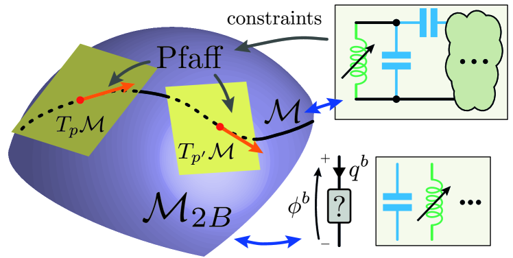
Figure 1: Sketch of the geometrical picture. There are two variables per branch, and they span $\mathcal{M}_{2B}$. Connecting the branches in a circuit gives rise to constraints, collected in a Pfaff system that fixes the possible directions at each point on $\mathcal{M}_{2B}$. The integration of those directions results in the integral manifold $\mathcal{M}$ that describes the constrained physics.

There is a natural conjugation between the flux and the charge of each branch, so $\mathcal{M}_{2B}$ is to be styled as a phase space or precursor thereof. However, there are constraints. Most importantly, the voltage and current Kirchoff constraints are a Pfaff system of equations for one forms [91] in $T^{*}\mathcal{M}_{2B}$,

$$\sum_{b\in\mathcal{N}}\mathrm{d}q^{b}=0\,\mathrm{(KCL)}\,,\qquad\sum_{b\in\mathcal{P}}\mathrm{d}\phi^{b}=0\,\mathrm{(KVL)}\,,$$ (1)

with $b\in\mathcal{N}$ denoting all branches incident on node $\mathcal{N}$ and $b\in\mathcal{P}$ all branches in loop $\mathcal{P}$. Because of the structure of $\mathcal{M}_{2B}$, this system is integrable, and the integral manifolds are of dimension $B$. Importantly, the number of charge type and flux type variables need not be equal, thus precluding the integral manifolds from being understood as phase spaces $T^{*}\mathcal{X}$ for some underlying configuration space $\mathcal{X}$. Hence the issues in all approaches to the construction of Hamiltonians for circuits of lumped elements, in one way or another. However, we know that large classes of circuits do indeed admit Hamiltonian descriptions. On reflection, we observe that the constructions for those descriptions are associated with the specific distribution of energetic elements of different types on specific graph structures, in intimate interplay with the topology of the circuit [28, 29].

Therefore, we consider circuits for which each branch belongs to one of the following categories, all of them ideal: linear and nonlinear capacitors ($\mathcal{C}$) and inductors ($\mathcal{L}$), voltage ($\mathcal{V}$) and current ($\mathcal{I}$) sources, linear resistors ($\mathcal{R}$), and transformer ($\mathcal{T}$) and gyrator ($\mathcal{G}$) branches. Only the reactive ($\mathcal{C}$ and $\mathcal{L}$) and source ($\mathcal{I}$ and $\mathcal{V}$) branches do actually present conjugate pairs of variables from the dynamical perspective, while the dissipative $\mathcal{R}$ set and the $\mathcal{T}$ and $\mathcal{G}$ sets will be constraints. The constitutive relations for capacitive $c\in\mathcal{C}$ and inductive $l\in\mathcal{L}$ branches are

$$\dot{\phi}^{c}=v^{c}=\frac{\partial h_{c}}{\partial q^{c}}\,,\qquad\dot{q}^{l}=i^{l}=\frac{\partial h_{l}}{\partial\phi^{l}}\,,$$ (2)

with a total energy function $H=\sum_{l\in\mathcal{L}}h_{l}(\phi^{l})+\sum_{c\in\mathcal{C}}h_{c}(q^{c})$. These relations seem to be half of a Hamiltonian pair, with opposing signs for capacitive and inductive elements. Thus, we associate a degenerate two-form on $\mathcal{M}_{2B}$ to the actual content of the circuit as

$$\begin{aligned} \omega_{2B}&=\frac{1}{2}\left[\sum_{l\in\mathcal{L}}\mathrm{d}\phi^{{l}}\wedge\mathrm{d}q^{l}+\sum_{c\in\mathcal{C}}\mathrm{d}q^{c}\wedge\mathrm{d}\phi^{{c}}\right]\\ &+\frac{1}{2}\left[\sum_{i\in\mathcal{I}}\mathrm{d}\phi^{{i}}\wedge\mathrm{d}q^{i}+\sum_{v\in\mathcal{V}}\mathrm{d}q^{v}\wedge\mathrm{d}\phi^{{v}}\right].\end{aligned}$$ (3)

Here, if necessary, we incur in the standard abuse of notation $\mathrm{d}\alpha$ for the winding one form in an $S^{1}$ variable, by writing it in terms of the angle $\alpha$ in one coordinate patch. We also associate a degenerate symmetric 2-covariant tensor field

$$g_{2B}=\frac{1}{2}\sum_{r\in\mathcal{R}}\mathrm{d}q^{r}\mathrm{d}\phi^{r}\,,$$ (4)

that encodes dissipation, and a source one form $\sigma$.

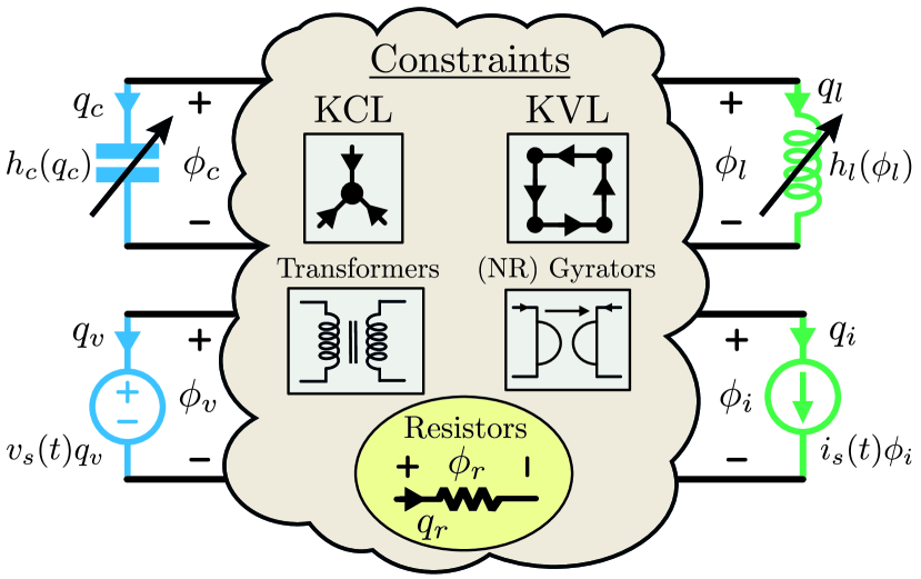
Figure 2: The lumped ideal elements under consideration. In the periphery the dynamical elements, determined by energy functions. Anticlockwise from the top right, inductor ($\mathcal{L}$), capacitor ($\mathcal{C}$), voltage source ($\mathcal{V}$) and current source ($\mathcal{I}$). In the cloud, various constraints govern the connection of dynamical elements, including Kirchhoff’s current (KCL) and voltage (KVL) laws, transformers ($\mathcal{T}$), gyrators ($\mathcal{G}$), and linear resistances ($\mathcal{R}$). The constitutive equations of the (multi-terminal) constraint elements can be expressed in the scattering matrix formalism $\mathsf{S}$, as systems of linear differential equations for charges and fluxes, $R\left[\mathsf{P}_{\alpha b}+\mathsf{S}_{\alpha b}\right]\mathrm{d}q^{b}=\left[\mathsf{P}_{\alpha b^{\prime}}-\mathsf{S}_{\alpha b^{\prime}}\right]\mathrm{d}\phi^{b^{\prime}}$, with $\mathsf{P}$ a projector onto the intervening branches.

The constraints $\mathcal{R}$, $\mathcal{T}$ and $\mathcal{G}$ that arise from connecting the elements, together with the Kirchoff constraints, constitute an external Pfaff system that, again, is integrable. The restriction (pullback under the immersion map $\imath:\mathcal{M}\to\mathcal{M}_{2B}$) of $\omega_{2B}$ to integral manifolds $\mathcal{M}$ of the Pfaff system is a (possibly degenerate) homogeneous closed two-form, $\omega=\imath^{*}\omega_{2B}$. The dimension of the final manifold $\mathcal{M}$, $\mathrm{dim}(\mathcal{M})=B-r_{P}\leq B$ depends on $r_{P}$, the relative rank of the resistor, transformer and gyrator constraint system with respect to the Kirchhoff constraints. The first central result of this work is that, in the absence of dissipation, the equations of motion that would follow from standard circuit theory, i.e. those that follow from the constitutive equations (2) when the constraints are imposed, are the same as the Euler–Lagrange equations of motion for the Lagrangian (using Einstein’s convention)

$$L=\frac{1}{2}\omega_{\alpha\beta}z^{\alpha}\dot{z}^{\beta}-H-S_{\alpha}{z}^{\alpha}\,,$$ (5)

with $z^{\alpha}$ coordinates in $\mathcal{M}$ and $\omega_{\alpha\beta}$ the matrix elements of the two-form. Generically the $z^{\alpha}$ coordinates need not be strictly node fluxes or loop charges. In fact, in the presence of non-reciprocal elements, with characteristic impedance parameter, they will be a mixture of those. The integration constants that determine an integral manifold will only appear through the energy function $H$, so they can generically be chosen such that the origin of coordinates is an energy minimum.

If there is dissipation, the equations are those derived from this Lagrangian together with the Rayleigh dissipation function determined by the restriction of $g_{2B}$.

3 Summary of the proof

The proof of the previous result hinges on the Tellegen properties of the constraints. The original Tellegen theorem is that for any network that describes an electrical circuit, the Kirchhoff constraints ensure that, independently of the actual dynamics, $\sum_{b}i^{b}v^{b}=0$. For our purposes this theorem is equivalent to the statement that the restriction of the symmetric 2-covariant tensor $\tau_{2B}=\sum_{b=1}^{B}\mathrm{d}\phi^{b}\mathrm{d}q^{b}$ to an integral manifold of a Pfaff external system that includes the Kirchhoff constraints is identically zero, $\imath^{*}\tau_{2B}=0$. If we have a restriction that satisfies this last equation we say that it presents the global Tellegen property. In contrast, the local Tellegen property concerns 2-covariant tensors that involve sums over a restricted set of branches, $\tau_{\mathcal{S}}=\sum_{s\in\mathcal{S}}\mathrm{d}\phi^{s}\mathrm{d}q^{s}$. The restriction from $\mathcal{M}_{2B}$ to $\mathcal{M}$ is said to have the local Tellegen property with respect to the set $\mathcal{S}$ if $\imath^{*}\tau_{\mathcal{S}}=0$. Crucially, the integral manifold for the Pfaff exterior system determined by the Kirchhoff, linear resistors, and transformer and gyrator constraints satisfies both the global Tellegen property and the local Tellegen properties with respect to $\mathcal{T}$ and $\mathcal{G}$. Once integrability and Tellegen have been established, the proof is algebraic, by identification of the circuit equations of motion with those derived from the Lagrangian (and Rayleigh function for dissipation).

Explicitly, with collective coordinates $\boldsymbol{\zeta}^{T}=(\operatorname{\boldsymbol{q}}^{T},\operatorname{\boldsymbol{\phi}}^{T})$, source vector $\boldsymbol{s}^{T}=(\operatorname{\boldsymbol{I}}^{T},\operatorname{\boldsymbol{V}}^{T})(t)$, and projectors $\mathsf{P}^{\mathcal{S}}$ selecting the branches in a set $\mathcal{S}$, the constitutive equations for capacitors, inductors and sources can be written compactly as

$$\begin{pmatrix}0&\mathsf{P}^{\mathcal{C}}+\mathsf{P}^{\mathcal{V}}\\ \mathsf{P}^{\mathcal{L}}+\mathsf{P}^{\mathcal{I}}&0\end{pmatrix}\dot{\boldsymbol{\zeta}}=\nabla_{\zeta}H+\begin{pmatrix}0&\mathsf{P}^{\mathcal{V}}\\ \mathsf{P}^{\mathcal{I}}&0\end{pmatrix}\boldsymbol{s}\,.$$ (6)

On the other hand, the solution of the constraint equations is given by a matrix $\mathsf{K}$, that connects the derivatives of the final variables $\mathbf{z}$ with those of $\boldsymbol{\zeta}$ in the pair

$$\begin{aligned} \dot{\boldsymbol{\zeta}}&=\mathsf{K}\dot{\mathbf{z}},\\ \nabla_{z}f&=\mathsf{K}^{T}\nabla_{\zeta}f.\end{aligned}$$ (7)

That is, $\mathsf{K}$ is the matrix that implements the pullback $\imath^{*}$ and $\mathsf{K}^{T}$ the one implementing the pushforward $\imath_{*}$. We compute it by codifying all the linear constraints as $\mathsf{F}\mathrm{d}\boldsymbol{\zeta}=0$, and computing the kernel of $\mathsf{F}$. A basis of this kernel is then collected as columns of the matrix $\mathsf{K}$, i.e. $\mathsf{FK}=0$. See more details for the explicit construction in Appendix A.

Thus, system (6) after the imposition of constraints becomes

$$\begin{aligned} \mathsf{K}^{T}\begin{pmatrix}0&\mathsf{P}\\ -\mathsf{P}&0\end{pmatrix}\mathsf{K}\dot{\mathbf{z}}=&\,\frac{1}{2}\mathsf{K}^{T}\begin{pmatrix}0&\mathsf{P}^{\mathcal{R}}\\ \mathsf{P}^{\mathcal{R}}&0\end{pmatrix}\mathsf{K}\dot{\mathbf{z}}+\nabla_{z}H\\ &+\mathsf{K}^{T}\begin{pmatrix}0&\mathsf{P}^{\mathcal{V}}\\ \mathsf{P}^{\mathcal{I}}&0\end{pmatrix}\boldsymbol{s}\,,\end{aligned}$$ (8)

where $\mathsf{P}=\mathsf{P}^{\mathcal{C}}+\mathsf{P}^{\mathcal{V}}+\left(\mathsf{P}^{\mathcal{R}}+\mathsf{P}^{\mathcal{G}}\right)/2$ and the global (Kirchhoff) and local ($\mathcal{T}$ and $\mathcal{G}$) Tellegen properties have been used. These are the equations of motion from Lagrangian (5) with Rayleigh dissipation function

$$\mathcal{F}=\frac{1}{2}\sum_{r\in\mathcal{R}}\dot{q}^{r}(z)\dot{\phi}^{r}(z)=\frac{1}{4}\dot{\mathbf{z}}^{T}\mathsf{K}^{T}\begin{pmatrix}0&\mathsf{P}^{\mathcal{R}}\\ \mathsf{P}^{\mathcal{R}}&0\end{pmatrix}\mathsf{K}\dot{\mathbf{z}}\,.$$ (9)

The source term in the Lagrangian is identified as

$$S_{\alpha}z^{\alpha}=\mathbf{z}^{T}\mathsf{K}^{T}\begin{pmatrix}0&\mathsf{P}^{\mathcal{V}}\\ \mathsf{P}^{\mathcal{I}}&0\end{pmatrix}\begin{pmatrix}\boldsymbol{I}(t)\\ \boldsymbol{V}(t)\end{pmatrix}\,.$$ (10)

For more details, refer to App. B.

4 Degenerate forms, the Faddeev-Jackiw method and quantization

We focus on the case without dissipation or sources, see App. C for further details. The two-form that appears in Lagrangian (5) is homogeneous by construction, and thus of homogeneous rank. If it is full rank, then it can be inverted and a local Darboux basis can be found by symplectic Gram–Schmidt [92]. If it is global one can proceed with standard canonical quantization. The generic case, however, is that the two-form is not full rank. For this reason we chose a first-order lagrangian formalism, Eq. (5), so as to apply the method of Faddeev and Jackiw [81, 82].

We identify the independent zero modes of the two-form $\omega$, a set of vectors $W=\left\{\boldsymbol{W}_{I}\right\}_{I=1}^{|W|}$, with cardinality $|W|=B-r_{P}-\mathrm{rank}(\omega)$. Contracting each zero mode with ${\mathrm{d}}H$ we obtain dynamical constraints $W_{I}=\boldsymbol{W}_{I}\cdot\nabla H=0$.

Some of these can be gauge constraints (i.e., identically satisfied) revealing redundancies in the description. If only Kirchhoff and transformer relations have been used to reach $\omega$, the gauge vectors are purely in charge or purely in flux directions, this not being the case for a dimensionful constraint. A charge (flux) gauge constraint signals an effective loop (cutset) in which only inductive (capacitive) elements take part.

In this first round of the method all $W_{I}$ constraints will be integrable, because $\omega$ is homogeneous, and therefore so are $\boldsymbol{W}_{I}$, and they commute. Thus there exists an associated integrable submanifold of $\mathcal{M}$. We now pull back the two-form to this reduced submanifold and repeat the analysis. If the new two-form has homogeneous full rank, then we have completed this process. Lastly, if homogeneous but not full rank, we compute its zero modes and repeat. The new vectors need no longer be homogeneous, and integrability is not a given. If the new two form is not homogeneous in rank we have a different type of obstruction. The process is repeated until either an obstruction is found or homogeneous full rank has been reached. Particular methods can exist for specific obstructions [85].

Summarizing, there are three types of obstruction, with different impact on quantization. First, lack of global Darboux coordinates or nontrivial topology of phase space, as in the $0-\pi$ qubit [93], giving rise to inequivalent quantizations [94, 95]. Second, nonhomogeneity in rank of $\omega$. In examples, as previously noted in [84] with the dual Dirac–Bergmann analysis, this is due to a bifurcation in the underlying classical system, that admits a Hamiltonian description, such that quantization might be possible in some cases, see further details in App. G. Third, nonintegrability of dynamical constraints, such that there is no classical Hamiltonian description.

5 Circuit examples

Let us illustrate this method to obtain Hamiltonians systematically by applying it to two circuit examples that would be singular, or defective, within the pure node-flux [27] or loop-charge methods [30], see Fig. 3. Further archetypal examples with voltage sources (modelling time-dependent external magnetic fluxes [96]) and resistances, as well as nonlinear singular circuits [84, 85] are treated in App. F.

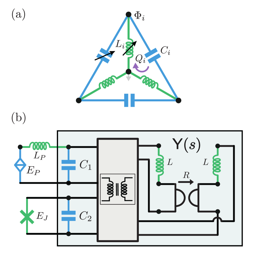
Figure 3: (a) The star circuit: a prototypical singular one. Conservation of current (inner node) and voltage (outer loop) may lead to reduction of variables. (b) Josephson and phase-slip junctions coupled to a 2-port nonreciprocal linear system described with an admittance matrix $\operatorname{\mathsf{Y}}(s)$, which is canonically-decomposed in a network of inductors, capacitors, gyrator and transformers.

5.1 Nonlinear star circuit

Consider the circuit in Fig. 3(a) with 3 nodes in a circle connected by capacitors forming a closed loop, and each of them connected to a common inner fourth node through inductors. We first apply our method to the linearized version of this circuit. Using as configuration space coordinates only node-flux variables $\Phi_{i}$ (loop-charge variables $Q_{i}$), the kinetic matrix $\tilde{\operatorname{\mathsf{C}}}$ ($\tilde{\operatorname{\mathsf{L}}}$) is singular, the Lagrangian is defective [27, 30], and no Hamiltonian can be obtained by Legendre transformation.

Following our method, the precanonical two-form (3) is $\omega_{2B}=\frac{1}{2}\left(\sum_{c}{\mathrm{d}}q_{c}\wedge{\mathrm{d}}\phi_{c}+\sum_{l}{\mathrm{d}}\phi_{l}\wedge{\mathrm{d}}\phi_{l}\right)$. We find a complete basis for charges and fluxes solving the kernel of $\operatorname{\mathsf{F}}_{\text{Kir}}$, which yields a basis of node-fluxes $\Phi_{i}$ and loop-charges $Q_{i}$ (uncoupled, given the fact that there are only reciprocal elements). Thus, $\omega=\imath^{*}\omega_{2B}$ becomes

$$\omega= \,{\mathrm{d}}Q_{1}\wedge\left({\mathrm{d}}\Phi_{1}-{\mathrm{d}}\Phi_{2}\right)+{\mathrm{d}}Q_{2}\wedge\left({\mathrm{d}}\Phi_{2}-{\mathrm{d}}\Phi_{3}\right)$$

$$+{\mathrm{d}}Q_{3}\wedge\left({\mathrm{d}}\Phi_{3}-{\mathrm{d}}\Phi_{1}\right).$$ (11)

that has zero vectors,

$$\mathbf{W}_{l} =\frac{\partial}{\partial\Phi_{1}}+\frac{\partial}{\partial\Phi_{2}}+\frac{\partial}{\partial\Phi_{3}}\,,$$ (12a)

$$\mathbf{W}_{c} =\frac{\partial}{\partial Q_{1}}+\frac{\partial}{\partial Q_{2}}+\frac{\partial}{\partial Q_{3}},$$ (12b)

associated with coordinates $w_{c}$ and $w_{l}$. Under the pertinent change of variables, we obtain $\omega={\mathrm{d}}Q_{a}\wedge{\mathrm{d}}\Phi_{a}+{\mathrm{d}}Q_{b}\wedge{\mathrm{d}}\Phi_{b}$, i.e., $\{\Phi_{\alpha},Q_{\beta}\}=\delta_{\alpha\beta}$. If all the elements are linear, the energy function in this Darboux basis $\{\xi^{\mu}\}\cup\{w^{I}\}\equiv(Q_{a},Q_{b},\Phi_{a},\Phi_{b},w_{c},w_{l})$ is written as

$$\begin{aligned} H=&\frac{{\left(Q_{a}+w_{c}\right)}^{2}}{2C_{1}}+\frac{w_{c}^{2}}{2C_{2}}+\frac{{\left(Q_{b}+w_{c}\right)}^{2}}{2C_{3}}\\ &+\frac{{\left(w_{l}+\phi_{2}\right)}^{2}}{2L_{1}}+\frac{{\left(w_{l}+\Phi_{a}+\Phi_{b}\right)}^{2}}{2L_{2}}+\frac{w_{l}^{2}}{2L_{3}}.\end{aligned}$$ (13)

Under elimination of the constraints, we derive the final Hamiltonian

$$H =\frac{1}{2}\left(\operatorname{\boldsymbol{Q}}^{T}\operatorname{\mathsf{C}}^{-1}\operatorname{\boldsymbol{Q}}+\operatorname{\boldsymbol{\Phi}}^{T}\operatorname{\mathsf{L}}^{-1}\operatorname{\boldsymbol{\Phi}}\right),$$ (14)

with $\operatorname{\mathsf{C}}^{-1}$ and $\operatorname{\mathsf{L}}^{-1}$ now full-rank $2\times 2$ matrices, see App. F.2 for all details of the computation. Naturally, this linear circuit is amenable to node-flux (loop-charge) quantization after making use of the star-mesh equivalence [97], followed by a subsequent reduction of one of the variables. It is worth emphasizing that this and all other linear reduction equivalences are inherently integrated into the method.

Next, let the third capacitor and the first inductor be nonlinear, with energy functions $h_{c}(q_{c3})$ and $h_{l}(\phi_{l1})$ respectively, with $q_{cj}$ the $j$-th capacitor’s branch charge and $\phi_{lj}$ the $j$-th inductor’s branch flux. There are two zero mode equations $\mathbf{W}_{c}(H)=\frac{q_{1}+w_{c}}{C_{1}}+\frac{w_{c}}{C_{2}}+h_{c}^{\prime}(q_{2}+w_{c})=0$, and $\mathbf{W}_{l}(H)=\frac{w_{l}+\phi_{1}+\phi_{2}}{L_{2}}+\frac{w_{l}}{L_{3}}-h_{l}^{\prime}(-(w_{l}+\phi_{2}))=0$, that implement charge and energy conservation for consistent reduction of the dynamics to two degrees of freedom. Under the conditions $h_{c}^{\prime\prime}(x)+\frac{1}{C_{1}}+\frac{1}{C_{2}}>0$ and $h_{l}^{\prime\prime}(-y)+\frac{1}{L_{2}}+\frac{1}{L_{3}}>0$, explicit solutions exist for the variables $w_{c}$ and $w_{l}$ in terms of these equations, resulting in a simplified Hamiltonian and canonical two-form, for two degrees of freedom, and canonical quantization follows. If not satisfied, this belongs to a more general class of singularities which are under active research [84, 85], see App. G.

5.2 Nonreciprocal blackbox-admittance quantization

As a second example, our method enables a natural extension of the highly effective black-box quantization approach [45, 47, 49] to nonreciprocal environments with multiple ports and poles. Consider the circuit in Fig. 3(b), a canonical nonreciprocal 2-port linear system with admittance matrix $\operatorname{\mathsf{Y}}(s)=\operatorname{\mathsf{D}}_{\infty}s+(\operatorname{\mathsf{D}}_{1}s+\operatorname{\mathsf{E}}_{1})/(s^{2}+\Omega_{1}^{2})$ [14] coupled to a Josephson junction and a phase-slip junction at the ports. Following our systematic method, we find that the two-form ($\omega=\imath^{*}\omega_{2B}$) is degenerate, with a single gauge zero mode. After its systematic elimination, we reach Hamiltonian

$$\begin{aligned} H=&\frac{1}{2}\left(\operatorname{\boldsymbol{q}}^{T}\operatorname{\mathsf{C}}^{-1}\operatorname{\boldsymbol{q}}+\operatorname{\boldsymbol{\phi}}^{T}\operatorname{\mathsf{L}}^{-1}\operatorname{\boldsymbol{\phi}}+\operatorname{\boldsymbol{q}}^{T}\operatorname{\mathsf{G}}\operatorname{\boldsymbol{\phi}}\right)\\ &+h_{P}(q_{1})+h_{J}(\phi_{2}),\end{aligned}$$ (15)

with three pairs of conjugate variables $\{\phi_{i},q_{j}\}=\delta_{ij}$, ready for canonical quantization. The computation is set out explicitly in App. F.3. Note that this Hamiltonian can be obtained with more effort by following the algebraic approach proposed in [32] with an adhoc method to eliminate transformer constraints followed by a Williamson’s reduction [98] of the nonreciprocal zero mode.

6 Conclusions & Outlook

In this article, we have developed a new and systematic method, fully programmable, to write the dynamics of general lumped-element electrical circuits, i.e., Kirchhoff’s and constitutive equations, as derived from a Lagrangian in first order and a Rayleigh dissipation function, following a consistent fully geometrical description. Using the Faddeev-Jackiw method, we identify and classify singularities. We provide a Hamiltonian description for all non-singular and for important classes of singular circuits. Our solution is based on the correct identification of the circuit-state degrees of freedom (mix of flux and charge variables), including both compact and extended ones. We have illustrated the method with pedagogical circuits with nonreciprocal and nonlinear elements, emphasizing those not susceptible to treatment or singular in a pure node-flux/loop-charge configuration space approach.

Further work will be required to add nonlinear dissipation to the classical dynamics of circuits within this scheme [19]. Finally, an extension to quasi-lumped element circuits [99, 78], as well as to construct fully quantum mechanical models of dissipation for quantized electrical networks, e.g., following the Caldeira-Leggett formalism [3, 27, 28, 100], should be natural by taking appropiate continuous limits of the models here obtained [56, 31].

Note: while finishing this manuscript we became aware of Ref. [101], which arrives at same results presented here for a more restricted class of circuits, i.e., with only non-dissipative (reciprocal) two-terminal elements.

Appendix A Constraints, geometry and algebra

Let us be explicit here about the construction of the embedding matrix $\mathsf{K}$, and illustrate it by way of a simple example. Moreover, this example will also show additional points of the process we want to stress later on.

First consider the case with purely Kirchhoff constraints. Since the work of Kirchhoff himself [76], the algebraic construction has been well established in terms of a pair of related matrices, the fundamental loop matrix $\mathsf{F}_{L}$ (please note that we use “loop” as is customary in the circuit literature to name what is termed “cycle” in the mathematical literature on graphs) and the fundamental cutset matrix $\mathsf{F}_{C}$, that furthermore satisfy the Tellegen property that $\mathsf{F}_{L}\mathsf{F}_{C}^{T}=0$. To obtain them, one selects a numbering of nodes, index $n$, and branches, index $b$, and an orientation of the branches in the graph that represents the lumped element circuit (the incorporation of graph theory to the analysis dates to Weyl [102]). The incidence matrix of the graph, $\mathsf{A}_{nb}$, will have rank $\mathrm{min}(N,B)-N_{C}=N-N_{C}$, where $N$ is the number of nodes, $B$ the number of branches, and $N_{C}$ the number of connected components of the graph. If the graph corresponds to a nontrivial circuit then there exists at least one loop, which implies $B\geq N$. The fundamental cutset matrix $\mathsf{F}_{C}$ is the reduced row echelon form by Gaussian elimination of this incidence matrix, after discarding the $N_{C}$ identically zero rows. For readers unfamiliar with these algebraic constructions, observe that they are equivalent to the identification of a minimal set of node fluxes that determine all branch voltage drops. The advantage of using this canonical form is clearly seen in the next step: this means that the kernel of $\mathsf{F}_{C}$ is readily constructed. Take a basis of this kernel space as vectors in $\mathbb{R}^{B}$. Writing the basis vectors in row form provides us with the fundamental loop matrix $\mathsf{F}_{L}$, and the Tellegen property $\mathbf{i}\cdot\mathbf{v}=0$ follows.

The Kirchoff constraints, written in a format that connects with the notations of this paper, are the statement

$$\mathsf{F}_{\mathrm{Kir}}{\mathrm{d}}\boldsymbol{\zeta}=\begin{pmatrix}\mathsf{F}_{C}&0\\ 0&\mathsf{F}_{L}\end{pmatrix}{\mathrm{d}}\boldsymbol{\zeta}=0\,,$$ (16)

which is a Pfaff exterior system. Solving these constraints means that we obtain a basis of the kernel space of $\mathsf{F}_{\mathrm{Kir}}$, and arrange its vectors as columns of a matrix $\mathsf{K}$, i.e. $\mathsf{F}_{\mathrm{Kir}}\mathsf{K}=0$. As we have chosen a canonical form for the Kirchhof constraints we can write $\mathsf{K}$ explicitly if those are the only constraints, namely

$$\mathsf{K}_{\mathrm{Kir}}=\begin{pmatrix}\mathsf{F}_{L}^{T}&0\\ 0&\mathsf{F}_{C}^{T}\end{pmatrix}\,.$$ (17)

Observe however that alternative algorithms exist and can be implemented systematically, were we not to start from a canonical form. As the Kirchhoff constraints separate in two sets, the current conservation constraint or Kirchhoff current law (KCL) on the one hand and the Kirchhoff voltage law on the other, the constrained manifold under just $\mathsf{F}_{\mathrm{Kir}}$ has clearly separated current and voltage directions.

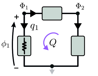
Figure 4: Series connection of three two-terminal lumped elements.

Consider for instance the graph associated with the circuit in Fig. 4. It is easy to construct the fundamental matrices in a canonical form,

$$\mathsf{F}_{C} =\begin{pmatrix}1&0&1\\ 0&1&-1\end{pmatrix}\,,$$ (18)

$$\mathsf{F}_{L} =\begin{pmatrix}1&-1&-1\end{pmatrix}\,.$$ (19)

The minimal set of variables that is required to describe all possible circuits constructed with the topology of Fig. 4 and one port elements is therefore composed of one loop charge and two node fluxes, and we have an explicit expression for $\mathsf{K}_{\mathrm{Kir}}$,

$${\mathrm{d}}\boldsymbol{\zeta}=\begin{pmatrix}{\mathrm{d}}\boldsymbol{q}\\ {\mathrm{d}}\boldsymbol{\phi}\end{pmatrix}=\begin{pmatrix}1&0&0\\ -1&0&0\\ -1&0&0\\ 0&1&0\\ 0&0&1\\ 0&1&-1\end{pmatrix}\begin{pmatrix}{\mathrm{d}}Q\\ {\mathrm{d}}\Phi_{1}\\ {\mathrm{d}}\Phi_{2}\end{pmatrix}\,.$$ (20)

This separated structure is also mantained if just transformer constraints are added to the mix, since a transformer fixes currents in terms of currents and voltages in terms of voltages, namely there exists a pair of matrices $\mathsf{T}$ and $\mathsf{T}^{\prime}$ such that $\mathsf{T}^{\prime}\mathsf{T}^{T}=0$ (local Tellegen property). Connecting with the projector notation that has been introduced in the main text (MT), observe that

$$\mathsf{T}\mathsf{P}^{\mathcal{T}}=\mathsf{T}$$ (21)

and similarly for $\mathsf{T}^{\prime}$. The Pfaff system they provide is

$$\mathsf{F}_{T}{\mathrm{d}}\boldsymbol{\zeta}=\begin{pmatrix}\mathsf{T}&0\\ 0&\mathsf{T}^{\prime}\end{pmatrix}{\mathrm{d}}\boldsymbol{\zeta}=0\,.$$ (22)

Therefore in a system in which we only have Kirchhoff and transformer constraints, the Pfaff system again partitions into a current set and a voltage set, and the computation of the kernel is facilitated by observing that in such a case

$$\mathrm{ker}\left(\mathsf{F}_{\mathrm{Kir}}\right)\cap\mathrm{ker}\left(\mathsf{F}_{\mathrm{T}}\right)=\mathrm{ker}\left(\mathsf{F}_{\mathrm{cur}}\right)\oplus\mathrm{ker}\left(\mathsf{F}_{\mathrm{vol}}\right)\,,$$ (23)

where

$$\mathsf{F}_{\mathrm{cur}} =\begin{pmatrix}\mathsf{F}_{C}\\ \mathsf{T}\end{pmatrix}\qquad\mathrm{and}$$ (24a)

$$\mathsf{F}_{\mathrm{vol}} =\begin{pmatrix}\mathsf{F}_{L}\\ \mathsf{T}^{\prime}\end{pmatrix}$$ (24b)

act on $\mathbb{R}^{B}$, unlike $\mathsf{F}_{\mathrm{Kir}}$ and $\mathsf{F}_{T}$, that act on $\mathbb{R}^{2B}$. Thus, under these conditions we are led to a description of the system in terms of effective loop charges and flux nodes (see to this point [49]). Concentrating on the effective loop charges, we determine those by again applying Gaussian reduction to $\mathsf{F}_{\mathrm{cur}}$ so that it is written in reduced row echelon form (discarding possible null rows),

$$\mathsf{F}_{\mathrm{cur}}\sim\begin{pmatrix}\mathbbm{1}_{B-\tilde{L}}&\tilde{\mathsf{A}}\end{pmatrix}\,.$$ (25)

Here $\tilde{\mathsf{A}}$ is a $\left(B-\tilde{L}\right)\times\tilde{L}$ matrix, and all currents are independently determined by $\tilde{L}$ effective loop charges $\left\{Q_{i}\right\}_{i=1}^{\tilde{L}}$,

$$\mathbf{i}=\begin{pmatrix}-\tilde{\mathsf{A}}\\ \mathbbm{1}_{\tilde{L}}\end{pmatrix}\begin{pmatrix}\dot{Q}_{1}\\ \vdots\\ \dot{Q}_{\tilde{L}}\end{pmatrix}\,.$$ (26)

The interpretation is that the number of independent cycles of the graph is reduced because of the transformer, and we are left with a set of effective independent cycles. An analogous construction holds for the effective node fluxes.

The separability of current and flux constraints for Kirchhoff and transformer constraints is reflected in the fact that these two cases are determined by pure numbers, incidences in the case of Kirchhoff, and turn ratios for transformers. On the other hand both resistor and gyrator constraints must include parameters with dimensions of impedance, as they do mix currents and voltages.

As a trivial example, imagine that the first branch of the example whose Kirchhoff constraints are realized in Eq. (20) is a resistence with constitutive equation $R{\mathrm{d}}q_{1}={\mathrm{d}}\phi_{1}={\mathrm{d}}\Phi_{1}$, see Fig.4. Then Eq. (20) is substituted by

$${\mathrm{d}}\boldsymbol{\zeta}=\begin{pmatrix}{\mathrm{d}}\boldsymbol{q}\\ {\mathrm{d}}\boldsymbol{\phi}\end{pmatrix}=\begin{pmatrix}1&0\\ -1&0\\ -1&0\\ R&0\\ 0&1\\ R&-1\end{pmatrix}\begin{pmatrix}{\mathrm{d}}Q\\ {\mathrm{d}}\Phi_{2}\end{pmatrix}\,.$$ (27)

More generally, if there are resistive elements there will be matrix elements with dimensions of either impedance or admittance in $\mathsf{K}$. However, if there are no non-reciprocal elements the final coordinates can be chosen as purely loop-charge or flux-node, as we see in the example.

In fact, the constraint elements (resistive, transformers and gyrators) can be described in a unified manner with the scattering matrix formalism, which we now briefly summarize. As stated in the MT, we partition the branches of the circuit graph in different sets with label $\mathcal{S}\in\left\{\mathcal{C},\mathcal{L},\mathcal{V},\mathcal{I},\mathcal{R},\mathcal{T},\mathcal{G}\right\}$, which denote, in sequence, capacitor, inductor, voltage source, current source, resistence, transformer, and gyrator. The set of constraint elements is $\mathcal{R}\cup\mathcal{T}\cup\mathcal{G}$. Then, acting on $T\mathcal{M}_{2B}$ homogenously, we have that for the subset $\mathcal{S}$ of the constraint element set the Pfaff system is

$$\mathsf{F}_{S}{\mathrm{d}}\boldsymbol{\zeta}=\begin{pmatrix}R\left(\mathsf{P}^{\mathcal{S}}+\mathsf{S}^{\mathcal{S}}\right)&|&\left(\mathsf{S}^{\mathcal{S}}-\mathsf{P}^{\mathcal{S}}\right)\end{pmatrix}{\mathrm{d}}\boldsymbol{\zeta}=0\,.$$ (28)

$R$ is a characteristic impedance, while the $\mathsf{S}^{\mathcal{S}}$ scattering matrices are adimensional. $\mathsf{P}^{\mathcal{S}}$ is the projector onto the $\mathcal{S}$ set. The scattering matrices $\mathsf{S}^{\mathcal{S}}$ satisfy

$$\mathsf{P}^{\mathcal{S}}\mathsf{S}^{\mathcal{S}}=\mathsf{S}^{\mathcal{S}}\mathsf{P}^{\mathcal{S}}=\mathsf{S}^{\mathcal{S}}\,.$$ (29)

The constraint is lossless if the scattering matrix is unitary, and reciprocal if it is symmetric. Ideal transformers are lossless and reciprocal, and therefore the eigenvalues of the corresponding scattering matrix (on its support space $\mathcal{S}$) are either $1$ or $-1$, which implies that they are correctly described by the $\mathsf{T}$ and $\mathsf{T}^{\prime}$ matrices mentioned earlier, satisfying the local Tellegen property. The separation between the $+1$ and $-1$ eigenspaces means that the impedance parameter drops out of the transformer constraint. An ideal gyrator, on the other hand, corresponds to the purely nonreciprocal part of a lossless scattering matrix, and therefore mixes the voltage and current variables, and the impedance parameter is required. Nonetheless, because it is lossless it satisfies the local Tellegen property. The simplest gyrator constraint, with two branches, is given by

$$\begin{pmatrix}i_{1}\\ i_{2}\end{pmatrix}=\frac{1}{R}\begin{pmatrix}0&1\\ -1&0\end{pmatrix}\begin{pmatrix}v_{1}\\ v_{2}\end{pmatrix}\,,$$ (30)

or, more compactly,

$$\mathbf{i}_{G}=\mathsf{Y}_{G}\mathbf{v}_{G}=\frac{1}{R}\,i\sigma^{y}\,\mathbf{v}_{G}\,,$$ (31)

where $\sigma^{y}$ is the imaginary Pauli matrix. More generally, the canonical form of a gyrator constraint matrix is

$$\mathsf{F}_{G}=\begin{pmatrix}\mathsf{P}^{\mathcal{G}}&|&-\mathsf{Y}_{G}\end{pmatrix}\,,$$ (32)

where the admittance matrix $\mathsf{Y}_{G}$ is real, satisfies $\mathsf{P}^{\mathcal{G}}\mathsf{Y}_{G}=\mathsf{Y}_{G}\mathsf{P}^{\mathcal{G}}=\mathsf{Y}_{G}$, and is antisymmetric on its support.

Thanks to the scattering matrix formalism we could unify all these ideal linear constraints into a single scattering matrix and a single impedance parameter, and that approach might prove useful in the automatization of our prescription. However, from a conceptual perspective and with a view to proving general statements it is convenient to present as separate transformer, gyrator, and linear resistive constraints.

Thus, the full set of Pfaff exterior equations that we consider will have the structure

$$\mathsf{F}{\mathrm{d}}\boldsymbol{\zeta}=\begin{pmatrix}\mathsf{F}_{\mathrm{Kir}}\\ \mathsf{F}_{T}\\ \mathsf{F}_{R}\\ \mathsf{F}_{G}\end{pmatrix}{\mathrm{d}}\boldsymbol{\zeta}=0\,.$$ (33)

As before, the task is to compute the kernel of $\mathsf{F}$ and collect a basis as column vectors in a matrix $\mathsf{K}$. Then $\mathsf{FK}=0$ will hold, and we express the embedding of the resulting integral manifold $\mathcal{M}$, with coordinates $z^{\alpha}$, by means of

$${\mathrm{d}}\boldsymbol{\zeta}=\mathsf{K}{\mathrm{d}}\mathbf{z}\,,$$ (34)

and correspondingly for the vectors

$$\nabla_{z}=\mathsf{K}^{T}\nabla_{\zeta}\,.$$ (35)

These coordinates will generally be neither loop-charge- nor node-flux-like. Rather they will mix them adequately.

Having achieved the description of all the branch variables, $\zeta$, in term of a set of prima facie independent ones, $z^{\alpha}$, we can now carry out the task of constructing $\omega$, by using the $\mathsf{K}$ matrix. As we shall now see, this simply means that

$$\omega_{\alpha\beta}=\left[\mathsf{K}\right]_{b\alpha}\left[\omega_{2B}\right]_{bb^{\prime}}\left[\mathsf{K}\right]_{b^{\prime}\beta}\,,$$ (36)

using coordinates.

The global and local Tellegen properties are the statements that

$$\begin{aligned} \mathsf{K}^{T}\begin{pmatrix}0&\mathbbm{1}\\ 0&0\end{pmatrix}\mathsf{K}&=\mathsf{K}^{T}\begin{pmatrix}0&\mathsf{P}^{\mathcal{T}}\\ \mathsf{P}^{\mathcal{T}}&0\end{pmatrix}\mathsf{K}\\ &=\mathsf{K}^{T}\begin{pmatrix}0&\mathsf{P}^{\mathcal{G}}\\ \mathsf{P}^{\mathcal{G}}&0\end{pmatrix}\mathsf{K}=0,\end{aligned}$$ (37)

together with their transposes. The first one is simply the statement that $\mathbf{i}\cdot\mathbf{v}$, for all possible $\mathbf{i}$ and $\mathbf{v}$ that satisfy the Kirchhoff constraint. As to the second one, observe that the matrix $\mathsf{T}$ we introduced above can be written in canonical right Belevitch [12, 103] form $\mathsf{T}\to\begin{pmatrix}\mathsf{N}&\mathbbm{1}\end{pmatrix}$ acting only on the branches in $\mathcal{T}$, and then similarly $\mathsf{T}^{\prime}\to\begin{pmatrix}\mathbbm{1}&-\mathsf{N}^{T}\end{pmatrix}$ on just the branches in $\mathcal{T}$. Here $\mathsf{N}$ is the turns ratio matrix. Then the currents and voltages in the branches of $\mathcal{T}$ must be of the form

$$\mathsf{P}^{\mathcal{T}}\mathbf{i} \to\begin{pmatrix}\mathbbm{1}\\ -\mathsf{N}\end{pmatrix}\tilde{\mathbf{I}}\qquad\mathrm{and}$$ (38)

$$\mathsf{P}^{\mathcal{T}}\mathbf{v} \to\begin{pmatrix}\mathsf{N}^{T}\\ \mathbbm{1}\end{pmatrix}\tilde{\mathbf{V}}\,,$$ (39)

for some $\tilde{\mathbf{I}}$ and $\tilde{\mathbf{V}}$, not necessarily generic, since other constraints will have to be fulfilled. From this structure it follows that $\left(\mathsf{P}^{\mathcal{T}}\mathbf{i}\right)\cdot\left(\mathsf{P}^{\mathcal{T}}\mathbf{v}\right)=0$. The local Tellegen property for $\mathcal{G}$ follows analogously from the definitions introduced by Tellegen [104], that required no dissipation for the ideal element. Alternatively, it flows from the unitarity of the scattering matrix $\mathsf{S}^{\mathcal{G}}$.

Appendix B Algebraic proof

The two-form $\omega_{2B}$ in Eq. (3) can be written more compactly as

$$\omega_{2B} =\frac{1}{2}{\mathrm{d}}\boldsymbol{q}^{T}\wedge\left(\mathsf{P}^{\mathcal{C}}+\mathsf{P}^{\mathcal{V}}-\mathsf{P}^{\mathcal{L}}-\mathsf{P}^{\mathcal{I}}\right){\mathrm{d}}\boldsymbol{\phi}$$

$$=\frac{1}{2}{\mathrm{d}}\boldsymbol{\zeta}^{T}\wedge\mathsf{E}_{2B}{\mathrm{d}}\boldsymbol{\zeta}\,,$$ (40)

with

$$\mathsf{E}_{2B}=$$ (41)

$$\frac{1}{2}\begin{pmatrix}0&\mathsf{P}^{\mathcal{C}}+\mathsf{P}^{\mathcal{V}}-\mathsf{P}^{\mathcal{L}}-\mathsf{P}^{\mathcal{I}}\\ -\mathsf{P}^{\mathcal{C}}-\mathsf{P}^{\mathcal{V}}+\mathsf{P}^{\mathcal{L}}+\mathsf{P}^{\mathcal{I}}&0\end{pmatrix},$$

which is the antisymmetric part of

$$\tilde{\mathsf{E}}_{2B}=\begin{pmatrix}0&\mathsf{P}^{\mathcal{C}}+\mathsf{P}^{\mathcal{V}}\\ \mathsf{P}^{\mathcal{L}}+\mathsf{P}^{\mathcal{I}}&0\end{pmatrix}\,,$$ (42)

precisely the matrix that appears in the constitutive equations, Eq. (6). The transformation $\mathsf{A}\to\mathsf{K}^{T}\mathsf{A}\mathsf{K}$ for an antisymmetric matrix is the expression in components of the pullback of a two-form by the immersion map $\imath:\mathcal{M}\to\mathcal{M}_{2B}$. Thus we see that the matrix acting on $\dot{\mathbf{z}}$ in the LHS of Eq. (8) is

$$\mathsf{K}^{T}{\mathsf{E}}_{2B}\mathsf{K}=\mathsf{K}^{T}\begin{pmatrix}0&\mathsf{P}\\ -\mathsf{P}&0\end{pmatrix}\mathsf{K}\,,$$ (43)

where $\mathsf{P}=\mathsf{P}^{\mathcal{C}}+\mathsf{P}^{\mathcal{V}}+\left(\mathsf{P}^{\mathcal{R}}+\mathsf{P}^{\mathcal{G}}\right)/2$ thanks to the global (Kirchhoff) and local ($\mathcal{T}$ and $\mathcal{G}$) Tellegen properties, Eq. (37) and its transposes.

For additional reference, we remind the reader that a Lagrangian $L(\left\{q^{i},\dot{q}^{i}\right\})$ and a Rayleigh dissipation function $\mathcal{F}(\left\{\dot{q}^{i}\right\})$ provide us with the equations of motion [105]

$$\frac{{\mathrm{d}}}{{\mathrm{d}}t}\left(\frac{\partial L}{\partial\dot{q}^{i}}\right)=\frac{\partial L}{\partial q^{i}}-\frac{\partial\mathcal{F}}{\partial\dot{q}^{i}}\,.$$ (44)

Appendix C The method of Faddeev and Jackiw

Both the original paper by Faddeev and Jackiw [81] and the later very pedagogical presentation by Jackiw [83] are good sources to understand the method. Nonetheless here we shall provide a brief introduction in support of application of the method to the analysis of electrical circuits.

The starting point is a first order lagrangian, that we write as

$$L=A_{\alpha}(z)\dot{z}^{\alpha}-H(z)\,.$$ (45)

The Euler–Lagrange equations of motion derived from this Lagrangian are

$$\omega_{\alpha\beta}(z)\dot{z}^{\beta}=\frac{\partial H}{\partial z^{\alpha}}\,,$$ (46)

with

$$\omega_{\alpha\beta}(z)=\frac{\partial A_{\beta}}{\partial z^{\alpha}}-\frac{\partial A_{\alpha}}{\partial z^{\beta}}\,.$$ (47)

It is frequently convenient to think in terms of differential forms, in which case we have

$$A =A_{\alpha}(z){\mathrm{d}}z^{\alpha}\,,$$ (48a)

$$\omega =\frac{1}{2}\omega_{\alpha\beta}{\mathrm{d}}z^{\alpha}\wedge{\mathrm{d}}z^{\beta}\,,$$ (48b)

$$\omega ={\mathrm{d}}A\,.$$ (48c)

If $\mathrm{det}(\omega)\neq 0$ everywhere we are in presence of the Hamiltonian equations of motion derived from Hamiltonian $H$ and Poisson bracket given by the inverse of the matrix $\omega$,

$$\left\{z^{\alpha},z^{\beta}\right\}=\omega^{\alpha\beta}\,,$$ (49)

with the convention than

$$\omega^{\alpha\beta}\omega_{\beta\gamma}=\delta^{\alpha}_{\gamma}\,.$$ (50)

However, as we shall see in circuital examples, it is frequently the case that $\mathrm{det}(\omega)=0$ in some locus. In the examples of interest to us we shall have $\omega$ homogeneous in the first step of the method, while inhomogeneous rank will possibly appear in later steps of the process.

At any rate, if $\mathrm{det}(\omega)=0$ somewhere (or everywhere) the motion is not guaranteed to be Hamiltonian. Let us consider the zero modes of $\omega$ at a singularity $p$ (which is implicit in the following, where required), $\left\{\mathbf{W}_{I}\right\}$. These are vector fields at $p$, such that for all vector fields $\mathbf{V}$ at the same point we have

$$\omega_{p}\left(\mathbf{W}_{I},\mathbf{V}\right)=0\,.$$ (51)

In coordinates, we have

$$\left(W_{I}\right)^{\alpha}\omega_{\alpha\beta}=\omega_{\alpha\beta}\left(W_{I}\right)^{\beta}=0\,.$$ (52)

Thus a zero mode of the two-form corresponds to a constraint, since using Eq. (52) with Eq. (46) entails the constraint

$$W_{I}=\left(W_{I}\right)^{\alpha}\frac{\partial H}{\partial z^{\alpha}}=0$$ (53)

at that point, where we define the value $W_{I}$ and, if $\mathrm{det}(\omega)=0$ holds in a region with homogeneous rank, $W_{I}$ is understood as a function on that region.

At this stage the question arises whether one can reduce the dimensionality of the problem by imposing the constraints. Let us assume that $\omega$ is of homogeneous rank. Then, locally, one can find coordinates $z\to\left\{w^{I}\right\}\cup\left\{\xi^{\mu}\right\}$ such that the constraints are

$$\frac{\partial H(\xi,w)}{\partial w^{I}}=0\,,$$ (54)

while the one form reads

$$A=\frac{1}{2}f_{\mu\nu}\xi^{\mu}\dot{\xi}^{\nu}\,,$$ (55)

and $f_{\mu\nu}$ is full rank. If $H$ is a nonlinear function of $w^{I}$ one can solve Eq. (54) for $w^{I}$. Thus, at this point, it is convenient to solve for as many as possible and reduce dimensions. Observe that the existence of these coordinates is guaranteed locally, and obstructions to a global reduction can exist for nontrivial topologies of $\mathcal{M}$. Furthermore, if the Hamiltonian were to dependend linearly on $w^{I}$ it is necessary to carry out additional steps.

There is an alternative approach in which instead of reducing the dimension of the dynamical system as above we treat all the constraints in the same manner, and introduce a new coordinate for each constraint. The reduction in dimensionality will be achieved obliquely, by identifying conserved quantities in the final Hamiltonian motion.

Both these procedures fail if, at some point in the iterations, $\omega$ is not of homogeneous rank. If the system under investigation is a physical model this situation will arise when there is a breakdown in the validity of the model.

Let us now examine the increase in dimensions associated with constraints. This is carried out by associating a new dimension to each constraint, and one form ${\mathrm{d}}\lambda^{I}$ dual to its tangent. Then we modify the one-fom $A$ as

$$A\to A+W_{I}{\mathrm{d}}\lambda^{I}\,,$$ (56)

leading to

$$\omega\to\omega+{\mathrm{d}}W_{I}\wedge{\mathrm{d}}\lambda^{I}\,.$$ (57)

Were this enlarged two-form nondegenerate, we would have achieved the goal of a Hamiltonian description for the dynamics. We have not pursued the increase in dimension route in this work, but do not exclude it being useful in particular circuital models in the future.

Appendix D Time dependent external magnetic fluxes and sources

There has been some discussion in the literature of superconducting circuits concerning the inclusion of external fluxes in their study (see, for instance, [96]). The main issue seems to be that there does not appear to be a unique prescription, and the doubts that this creates as to the uniqueness of their description. Here we study this question from our perspective. The results are, first, that indeed there is freedom, as in many other steps of the process, yet, because of the underlying geometric structure, the physics in all choices is equivalent, and, two, that gauge variables might appear, and can be eliminated as part of our procedure.

The central point to be made is that an external flux is univocally associated with a loop in the circuit. Thus a prescription, illustrated in Fig. 5, for describing an external flux in terms of a voltage source goes as follows:

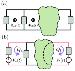
Figure 5: a) Fluxes $\Phi^{e}_{1}$ and $\Phi^{e}_{2}$ thread a circuit, and are represented b) by voltage sources $V_{a}$ and $V_{b}$ corresponding to the loop charges, with the external fluxes being partitioned into sources according to a cycle decomposition.

1. Choose a tree and a corresponding chord set to carry out the Kirchhoff constraint analysis, before imposing transformer and gyrator constraints. Each chord corresponds to a unique loop, and any loop can be written as a linear superposition of the chord loops.

2. Specifically, the choice of a tree means that the fundamental cutset matrix has been identified and has been written in Gauß–Jordan form as $\begin{pmatrix}\mathbbm{1}&\mathsf{A}_{\mathrm{chord}}\end{pmatrix}$. In particular, this also entails that the branches have been ordered in such a way that the chords are the last branches to be enumerated. The loop basis is given by the column matrices of

   $$\mathsf{B}_{\mathrm{loop}}=\begin{pmatrix}-\mathsf{A}_{\mathrm{chord}}\\ \mathbbm{1}\end{pmatrix}\,.$$ (58)

   Let us denote those column vectors by $\mathbf{c}_{i}$, where $i$ ranges from 1 to the number of chords.

3. Given an external flux, the associated loop is given by a sequence of edges. These edges are oriented according to the sign of the flux, and the flux loop is expressed with a column vector with entries $\pm 1$, if the corresponding edge is in the loop, or 0 otherwise. Let $\mathbf{l}$ be that column vector. If there is more than one external flux let $e$ be an index for the fluxes, $\Phi^{e}(t)$, and denote the corresponding loop vectors as $\mathbf{l}_{e}$.

4. Now compute the coefficients of $\mathbf{l}_{e}$ in the basis $\left\{\mathbf{c}_{i}\right\}$,

   $$\mathbf{l}_{e}=L_{e}^{\phantom{e}i}\mathbf{c}_{i}\,.$$ (59)

   We now see that we can expand the flux vector $\Phi^{e}\mathbf{l}_{e}$ in the loop basis,

   $$\Phi^{e}\mathbf{l}_{e}=\tilde{\Phi}^{i}\mathbf{c}_{i}=\Phi^{e}L_{e}^{\phantom{e}i}\mathbf{c}_{i}\,,$$ (60)

   using this to define its components in that basis, $\tilde{\Phi}^{i}=\Phi^{e}L_{e}^{\phantom{e}i}$.

5. Starting from the previous directed graph $G$ that describes the circuit $C$, we now obtain a new graph $G^{\prime}$ (and a new circuit $C^{\prime}$) by breaking each chord into two edges (i.e. inserting a new node per chord), with one of the edges retaining its previous character (capacitive, inductive, transformer branch…) and the other becoming a voltage source, with voltage function $V_{i}(t)=\dot{\tilde{\Phi}}^{i}$. We are working in the maximal case in which none of the $\tilde{\Phi}^{i}$ are zero. If there are zeroes, then we do not break that chord, and the subsequent counting has to be properly modified, without changing the result in any essential way. We continue the description only with the maximal case. Observe that alternatives exist. For instance, instead of breaking a chord sometimes it is more convenient (and equivalent) to break a node into two and having the new connecting branch be the source branch. We shall actually use this alternative in a later example, Fig. 9 in section F.4.

6. By following this procedure we have created a new circuit with a new number of branches, $B^{\prime}$, and nodes $N^{\prime}$, so we have increased the dimension of the initial manifold to $2B^{\prime}$. The number of components, $P$, does not change. Let the number of chords of the initial circuit be denoted by $C_{h}$, and correspondingly the number of chords of the resulting circuit by $C_{h}^{\prime}$. Then we have the following set of relations that issue from the procedure:

   $$C_{h} =B-N+P\,,$$

   $$B^{\prime} =B+C_{h}=2B-N+P\,,$$ (61)

   $$N^{\prime} =N+C_{h}=B+P\,,$$

   $$C_{h}^{\prime} =B^{\prime}-N^{\prime}+P=C_{h}\,.$$

7. The rank of the initial two form $\omega_{2B}$ is also modified, in that

   $$\mathrm{rank}\left(\omega_{2B^{\prime}}\right)=\mathrm{rank}\left(\omega_{2B}\right)+2(B-N+P)\,,$$

   as we have introduced one conjugate pair per (broken) chord.

8. However, it is clear that there will be redundancies: in a language adequate for Kirchhoff constraints, we have not increased the number of loop charges, which is still $C_{h}$, but we have increased the number of nodal fluxes to $N^{\prime}-P$. Therefore, on imposing the linear constraints, now on $\mathcal{M}^{2B^{\prime}}$, the resulting presymplectic form might have additional zero modes. Even more, some of those zero modes will be gauge modes. By this we mean that the constraint function built as $\Omega_{v}=\mathbf{v}\cdot\nabla_{z}H$ for the zero mode $\mathbf{v}$ is identically zero on the constraint. In many cases it can be imposed directly and reduce the system. Otherwise, gauge fixing might be required.

9. It is important to observe that these gauge modes will also appear for other choices of tree and chords in the initial circuit. The result of the procedure is independent, from the physics point of view, of the choice of tree and chords for imposing Kirchhoff constraints. In fact, our description of the procedure is completely independent of the character of the chord being split upt. Admittedly, there are choices in which the number of gauge modes is smaller: if the chord is inductive then there will be a gauge mode, but not so for the capacitive case. Nonetheless, the procedure is systematic and allows the identification of these modes.

As a final comment, observe that alternative prescriptions exist, in which the Kirchhoff constraints are rewritten to be no longer linear, but affine. This perspective could be brought to use in a contact geometric analysis, as well. However, as we show in the next section, the specificity of the dynamical systems associated to the class of circuits under consideration means that contact geometry is not required, and thus we provide this recipe that mantains the Kirchhoff constraints as linear.

Appendix E Dynamical constraints in presence of sources and dissipation

In this work we are studying the equations of motion for a lumped element circuit whose reactive elements are capacitors and inductors, resistences are linear, and possibly with ideal transformers and gyrators, and we have showed that they can be written as derived from a first order lagrangian and a quadratic Rayleigh dissipation function,

$$L =\frac{1}{2}\omega_{\alpha\beta}z^{\alpha}\dot{z}^{\beta}-H-S_{\alpha}{z}^{\alpha}\,,$$ (62a)

$$\mathcal{F} =\frac{1}{2}\sum_{r\in\mathcal{R}}\dot{q}^{r}\dot{\phi}^{r}=\frac{1}{2}\mathcal{F}_{\alpha\beta}\dot{z}^{a}\dot{z}^{\beta}\,,$$ (62b)

where the coefficients of the Rayleigh function are

$$\mathcal{F}_{\alpha\beta}=\frac{1}{2}\left[\mathsf{K}^{T}\begin{pmatrix}0&\mathsf{P}^{\mathcal{R}}\\ \operatorname{\mathsf{P}}^{\mathcal{R}}&0\end{pmatrix}\mathsf{K}\right]_{\alpha\beta}\,.$$ (63)

As mentioned above and shown in examples, generically $\omega$ is degenerate, and this gives rise to constraints that can be analyzed with the Faddeev–Jackiw method in the absence of sources and dissipation. Here we shall extend the analysis of dynamical constraints to those cases.

To do so, observe that the equations of motion can be written in the form

$$\left(\omega_{\alpha\beta}-\mathcal{F}_{\alpha\beta}\right)\dot{z}^{\beta}=\frac{\partial}{\partial z^{\alpha}}\left[H+S_{\beta}z^{\beta}\right]\,.$$ (64)

Therefore, if (with obvious notation) the matrix $\omega-\mathcal{F}$ is invertible we have a system of ordinary differential equations, non-autonomous if $S_{\beta}$ are time-dependent, and all variables $z^{\alpha}$ are dynamical. Observe that if $\omega$ is degenerate and $\omega-\mathcal{F}$ is invertible the system is only amenable to a Hamiltonian plus dissipation description by enlarging the phase space.

On the other hand, if $\omega-\mathcal{F}$ is not invertible we have (time-dependent) constraints, that must be imposed consistently. Namely, let $W^{\alpha}$ be the components of a left zero-vector of $\omega-\mathcal{F}$,

$$W^{\alpha}\left(\omega_{\alpha\beta}-\mathcal{F}_{\alpha\beta}\right)=0\,.$$ (65)

Then the following condition is a dynamical constraint on the system of equations in Eq. (64),

$$W^{\alpha}\frac{\partial}{\partial z^{\alpha}}\left[H+S_{\beta}z^{\beta}\right]=0\,,$$ (66)

in lieu of the FJ constraint (53). A local coordinatization will again exist in terms of the degenerate ($w$) and non-degenerate ($\xi$) directions, and the dynamical constraint is the requirement of independence of the total energy function $H+S_{\beta}z^{\beta}$ with respect to the degenerate directions. If the constraints are solvable we will obtain a reduced dynamical system. Generally this dynamical system will not be Hamiltonian, and non-Hamiltonian techniques will be required for further analysis. At any rate, our description allows for an identification of the actual dynamical content of the circuit description.

Let us now concentrate on the non-dissipative case with sources. In this case an extension of the Faddeev–Jackiw is possible, with subtleties. The issue of time dependent constraints has been examined in the literature, both from the Dirac–Bergmann [106, 107, 108] and the Faddeev–Jackiw [109] perspectives. We give a general description first, then we compute a couple of simple examples in our context, and we finish this section with a general discussion of FJ reduction for our nondissipative circuits. The starting point is the (pre-)contact structure, defined on $\mathcal{M}\times\mathbb{R}$, where the real line is the time parameter,

$$\Omega_{c}=\omega+{\mathrm{d}}\left(H+S_{\alpha}(t)z^{\alpha}\right)\wedge{\mathrm{d}}t\,.$$ (67)

For the systems under study, with equations of motion

$$\omega_{\alpha\beta}\dot{z}^{\beta}=\frac{\partial H}{\partial z^{\alpha}}+S_{\alpha}(t)\,,$$ (68)

the two-form $\Omega_{c}$ is an integral invariant. If we have a set of time independent constraints that determine a submanifold $\mathcal{M}^{\prime}\subset\mathcal{M}$ at all times, then there is a pullback of the contact form that has the same structure, with the pullback of $\omega$ and the time dependent energy function separately. However, if there exist time dependent constraints there will be an additional term in the pullback of $\Omega_{c}$, of the form $B\wedge{\mathrm{d}}t$, and unless $B$ is a closed form modulo ${\mathrm{d}}t$ we cannot understand the evolution as Hamiltonian. More concretely, let the embedding be, in coordinates, $z^{\alpha}(\xi^{\mu},t)$. Then the one form $B$ is

$$B=-\omega_{\alpha\beta}\frac{\partial z^{\alpha}}{\partial t}\frac{\partial z^{\beta}}{\partial\xi^{\mu}}{\mathrm{d}}\xi^{\mu}\,.$$ (69)

Thus, explicitly, ${\mathrm{d}}B$ is

$${\mathrm{d}}B =\frac{\partial}{\partial\xi^{\nu}}\left[\omega_{\alpha\beta}\frac{\partial z^{\alpha}}{\partial t}\frac{\partial z^{\beta}}{\partial\xi^{\mu}}\right]{\mathrm{d}}\xi^{\mu}\wedge{\mathrm{d}}\xi^{\nu}$$

$$\,+\frac{\partial}{\partial t}\left[\omega_{\alpha\beta}\frac{\partial z^{\alpha}}{\partial t}\frac{\partial z^{\beta}}{\partial\xi^{\mu}}\right]{\mathrm{d}}\xi^{\mu}\wedge{\mathrm{d}}t\,,$$ (70)

which means that $B$ is locally closed module ${\mathrm{d}}t$ if the first term is zero. If $B$ is locally closed modulo ${\mathrm{d}}t$ and there are no global obstructions (which could be the case in presence of compact variables), then we can determine a function $K$ such that $B={\mathrm{d}}K$ modulo ${\mathrm{d}}t$. Let us additionally assume that the pullback of $\omega$ is nondegenerate. Then the evolution under the constraints is Hamiltonian, with complete Hamiltonian $H+S_{\mu}\xi^{\mu}+K$.

Let us show a simple example in which there are no issues, that of a voltage driven LC oscillator.

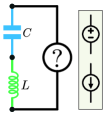
Figure 6: Series LC oscillator driven by a voltage or a current source. These systems can be described with a time-dependent Hamiltonian derived from the method, by imposing a constraint.

The circuit graph is a ring with three branches and three nodes, as represented in Fig. 6. Applying our systematic procedure we have three variables, $\mathbf{z}^{T}=\begin{pmatrix}Q&\Phi&w\end{pmatrix}^{T}$, with two-form

$$\omega={\mathrm{d}}Q\wedge{\mathrm{d}}\Phi$$ (71)

and total energy function $h_{1}(Q)+h_{2}(\Phi)+QV(t)$. The zero-mode coordinate $w$ does not appear anywhere, the correspoding constraint $\partial_{w}(H+QV)=0$ is automatically satisfied and we have a Hamiltonian system, with canonical coordinates.

The situation is a bit more involved if it is a current source instead of a voltage source. In that case the null direction for the two form is again a coordinate $w$, the two form is again (71). The total energy function is however $h_{1}(Q)+h_{2}(w-\Phi)-wI(t)$. Thus there is a nontrivial constraint, namely $I(t)=h_{2}^{\prime}(w-\Phi)$, which is to be solved for $w$. Then the system is Hamiltonian under the substitution of $w$ by its constrained value.

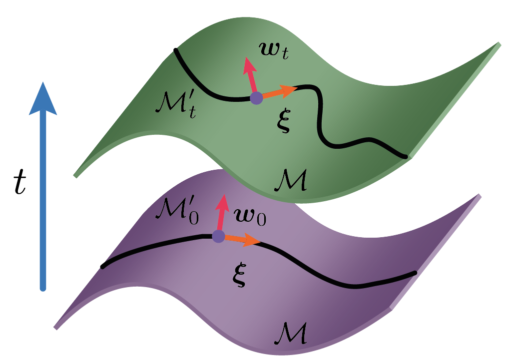
Figure 7: The manifold $\mathcal{M}$ is restricted by a time dependent constraint to a submanifold $\mathcal{M}^{\prime}_{t}$ at time $t$. The constraint is made explicit by solving $w^{I}$ as functions of $\xi^{\mu}$ and $t$. Because $\omega$ is homogeneous and time independent, the coordinates $\xi^{\mu}$ can always describe $\mathcal{M}^{\prime}_{t}$ for all times $t$.

Let us now show that the FJ reduction we explained in section C is directly applicable in our context. For an illustration of the geometric setup, see Fig. 7. In a nutshell, in the context of circuits $B$ is identically zero, and thus trivially closed. In the systems of interest, as we have indicated above, $\omega$ constructed from our algorithm is homogeneous. If it is singular, its zero directions have associated coordinates $w^{I}$, and $\omega$ is nondegenerate in directions associated with coordinates $\xi^{\mu}$. In other words,

$$\omega=\frac{1}{2}f_{\mu\nu}{\mathrm{d}}\xi^{\mu}\wedge{\mathrm{d}}\xi^{\nu}\,,$$ (72)

with homogeneous $f_{\mu\nu}$. The constraints are

$$\frac{\partial}{\partial w^{I}}\left(H(\xi,w)+S_{\mu}\xi^{\mu}+S_{I}w^{I}\right)=0\,,$$ (73)

and we determine $w^{I}(\xi,t)$ hence, if possible. The coordinates $\xi^{\mu}$ are free, and in fact are the coordinates for $\mathcal{M}^{\prime}_{t}$ (at each instant of time). Therefore $B=0$. It follows that, if we can solve $w^{I}$ from the constraints (73), we can effect Hamiltonian reduction in this case.

Appendix F Examples

In this section, we utilize our method to construct systematically (extended) Lagrangian and Hamiltonian dynamics of circuits containing all the lumped elements introduced in the main text. In doing so, we recover standard results from flux-node [27, 28] or loop-charge analysis [30], as well as more general (nonreciprocal) black-box analysis [45, 49, 59, 61].

F.1 RLC circuit

Figure 8: Parallel RLC circuit. In the classical depiction there are two loops and one active node involved in general. The resistor is considered a constraint, allowing the formulation of dynamical equations using just one set of paired conjugate variables.

The formalism we have presented includes the systematic treatment of linear resistences, making use of the Rayleigh dissipation function formalism [58]. To illustrate this point and to give a very simple example we now consider the parallel RLC circuit, depicted in Fig. 8. We choose to order the three parallel branches as the sequence capacitor/inductor/resistor. The cutset matrix and resistence constraint matrix are

$$\operatorname{\mathsf{F}}_{C} =\begin{pmatrix}1&1&1\end{pmatrix},$$ (74)

$$\operatorname{\mathsf{F}}_{R} =\begin{pmatrix}0&0&R&0&0&-1\end{pmatrix}$$ (75)

to construct $\operatorname{\mathsf{F}}$, with kernel

$$\operatorname{\mathsf{K}}=\begin{pmatrix}1&0\\ 0&1\\ -1&-1\\ -R&-R\\ -R&-R\\ -R&-R\end{pmatrix}$$ (76)

such that we have two independent charges $\mathbf{z}^{T}=\begin{pmatrix}Q_{1}&Q_{2}\end{pmatrix}^{T}$, and the precanonical two-form is simply

$$\operatorname{\mathsf{E}}_{2B}=\begin{pmatrix}0&0&0&1&0&0\\ 0&0&0&0&0&0\\ 0&0&0&0&0&\frac{1}{2}\\ -1&0&0&0&0&0\\ 0&0&0&0&0&0\\ 0&0&-\frac{1}{2}&0&0&0\end{pmatrix}.$$ (77)

Mapping to the reduced manifold,

$$\operatorname{\mathsf{E}}=\operatorname{\mathsf{K}}^{T}\operatorname{\mathsf{E}}_{2B}\operatorname{\mathsf{K}}=\begin{pmatrix}0&-R\\ R&0\end{pmatrix}\,$$ (78)

or, equivalently, $\{Q_{1},Q_{2}\}=R$. The Hamiltonian reads

$$H=\frac{Q_{1}^{2}}{2C}+R^{2}\frac{{\left(Q_{1}+Q_{2}\right)}^{2}}{2L}\,,$$ (79)

while the dissipation function is, in these coordinates,

$$\mathcal{F}=\frac{R}{2}\left(\dot{Q}_{1}+\dot{Q}_{2}\right)^{2}\,.$$ (80)

The equations of motion, as there are no sources, are in matrix form

$$\mathsf{E}\dot{z}=\nabla_{z}H+\nabla_{\dot{z}}\mathcal{F}\,,$$ (81)

and thus one obtains

$$-R\dot{Q}_{2} =\frac{Q_{1}}{C}+\frac{R^{2}}{L}\left(Q_{1}+Q_{2}\right)+R\left(\dot{Q}_{1}+\dot{Q}_{2}\right)\,,$$ (82)

$$R\dot{Q}_{1} =\frac{R^{2}}{L}\left(Q_{1}+Q_{2}\right)+R\left(\dot{Q}_{1}+\dot{Q}_{2}\right)\,.$$ (83)

To reach this point, a number of choices have been made, namely for the ordering of nodes and branches, and the basis for the kernel of $\mathsf{F}$. It should be clear that the actual dynamics would be recovered under different ones, as the prescription is univocal in that regard. Indeed, that is precisely the main reason to use a Hamiltonian description, namely to increase the set of possible variables so as to have more tools to understand and, where possible, solve the dynamics. To make this point more apparent, let us carry out an additional change of variables,

$$\begin{pmatrix}Q_{1}\\ Q_{2}\end{pmatrix}=\begin{pmatrix}1&0\\ -1&-1/R\end{pmatrix}\begin{pmatrix}Q\\ \Phi\end{pmatrix}\,.$$ (84)

In terms of these new variables, we read directly the harmonic oscillator Hamiltonian

$$H=\frac{Q^{2}}{2C}+\frac{{\Phi}^{2}}{2L},$$ (85)

canonical commutator $\left\{\Phi,Q\right\}=1$, and dissipation function

$$\mathcal{F}=\frac{\dot{\Phi}^{2}}{2R}= \,\frac{1}{2}\begin{pmatrix}\dot{Q}&\dot{\Phi}\end{pmatrix}\begin{pmatrix}1&-1\\ 0&-\frac{1}{R}\end{pmatrix}\times\dots$$ (86)

$$\dots\times\begin{pmatrix}R&R\\ R&R\end{pmatrix}\begin{pmatrix}1&0\\ -1&-1/R\end{pmatrix}\begin{pmatrix}\dot{Q}\\ \dot{\Phi}\end{pmatrix}$$

such that the equations of motion, Eq. (6), are directly computed from the final Hamiltonian, Poisson bracket, and dissipation function,

$$\dot{\Phi} =\frac{\partial H}{\partial Q}+\frac{\partial\mathcal{F}}{\partial\dot{Q}}=\frac{Q}{C}\,,$$ (87)

$$\dot{Q} =-\frac{\partial H}{\partial\Phi}-\frac{\partial\mathcal{F}}{\partial\dot{\Phi}}=-\frac{\Phi}{L}-\frac{\dot{\Phi}}{R}\,.$$

Naturally we recover the elementary RLC description of a damped harmonic oscillator, as was only to be expected.

F.2 The star circuit

A cutset matrix for the star circuit in Fig. 3(a) with $N=4$ nodes and $B=6$ branches is

$$\operatorname{\mathsf{F}}_{C}=\begin{pmatrix}1&0&-1&1&0&0\\ -1&1&0&0&1&0\\ 0&-1&1&0&0&1\end{pmatrix},$$ (88)

where the first (last) three columns correspond to the capacitor (inductor) branches with kernel

$$\operatorname{\mathsf{K}}=\begin{pmatrix}1&0&0&0&0&0\\ 0&1&0&0&0&0\\ 0&0&1&0&0&0\\ -1&0&1&0&0&0\\ 1&-1&0&0&0&0\\ 0&1&-1&0&0&0\\ 0&0&0&1&-1&0\\ 0&0&0&0&1&-1\\ 0&0&0&-1&0&1\\ 0&0&0&1&0&0\\ 0&0&0&0&1&0\\ 0&0&0&0&0&1\end{pmatrix},$$ (89)

such that the two-form matrix representation is

$$\operatorname{\mathsf{E}}=\operatorname{\mathsf{K}}^{T}\operatorname{\mathsf{E}}_{2B}\operatorname{\mathsf{K}}= \begin{pmatrix}0&0&0&1&-1&0\\ 0&0&0&0&1&-1\\ 0&0&0&-1&0&1\\ -1&0&1&0&0&0\\ 1&-1&0&0&0&0\\ 0&1&-1&0&0&0\end{pmatrix}$$ (90)

$$\sim\begin{pmatrix}0&0&1&0&0&0\\ 0&0&0&1&0&0\\ -1&0&0&0&0&0\\ 0&-1&0&0&0&0\\ 0&0&0&0&0&0\\ 0&0&0&0&0&0\end{pmatrix},$$ (91)

where the second line is written in the Darboux basis under a linear (point) transformation of coordinates. The null eigenspace of $\operatorname{\mathsf{E}}$ corresponding to the voltage and current constraints in the outer loop and inner node, respectively, is expanded by

$$\mathbf{W}_{l}=\begin{pmatrix}0\\ 0\\ 0\\ 1\\ 1\\ 1\end{pmatrix},\quad\mathbf{W}_{c}=\begin{pmatrix}1\\ 1\\ 1\\ 0\\ 0\\ 0\end{pmatrix}.$$ (92)

Alternatively, we could start from the loop charges and the node fluxes depicted in Fig. 3(a), since we know that they suffice to express all branch charges and fluxes, and obtain the two-form

$$\omega ={\mathrm{d}}Q_{1}\wedge\left({\mathrm{d}}\Phi_{1}-{\mathrm{d}}\Phi_{2}\right)$$

$$\quad+{\mathrm{d}}Q_{2}\wedge\left({\mathrm{d}}\Phi_{2}-{\mathrm{d}}\Phi_{3}\right)$$ (93)

$$\quad+{\mathrm{d}}Q_{3}\wedge\left({\mathrm{d}}\Phi_{3}-{\mathrm{d}}\Phi_{1}\right)\,,$$

with zero vectors

$$\mathbf{W}_{l} =\frac{\partial}{\partial\Phi_{1}}+\frac{\partial}{\partial\Phi_{2}}+\frac{\partial}{\partial\Phi_{3}}\,,$$ (94a)

$$\mathbf{W}_{c} =\frac{\partial}{\partial Q_{1}}+\frac{\partial}{\partial Q_{2}}+\frac{\partial}{\partial Q_{3}}\,.$$ (94b)

The Darboux basis above corresponds to the change of variables

$$\begin{aligned} Q_{1}&=Q_{a}+w_{c},&\quad\Phi_{1}&=-(w_{l}+\Phi_{b})\\ Q_{2}&=w_{c},&\quad\Phi_{2}&=-(w_{l}+\Phi_{a}+\Phi_{b})\\ Q_{3}&=Q_{b}+w_{c},&\quad\Phi_{3}&=-w_{l},\end{aligned}$$ (95)

such that $\omega={\mathrm{d}}Q_{a}\wedge{\mathrm{d}}\Phi_{a}+{\mathrm{d}}Q_{b}\wedge{\mathrm{d}}\Phi_{b}$. Considering, as in the MT, that all the elements are linear, the Hamiltonian in this Darboux basis $\{\xi^{\mu}\}\cup\{w^{I}\}\equiv(Q_{a},Q_{b},\Phi_{a},\Phi_{b},w_{c},w_{l})$ is written as

$$\begin{aligned} H=&\,\frac{{\left(Q_{a}+w_{c}\right)}^{2}}{2C_{1}}+\frac{w_{c}^{2}}{2C_{2}}+\frac{{\left(Q_{b}+w_{c}\right)}^{2}}{2C_{3}}\\ &+\frac{{\left(w_{l}+\phi_{2}\right)}^{2}}{2L_{1}}+\frac{{\left(w_{l}+\Phi_{a}+\Phi_{b}\right)}^{2}}{2L_{2}}+\frac{w_{l}^{2}}{2L_{3}}.\end{aligned}$$ (96)

We can now solve the zero mode constraints (54) $w_{l}$ and $w_{c}$, and arrive to the quantizable Hamiltonian

$$H =\frac{1}{2}\left(\operatorname{\boldsymbol{Q}}^{T}\operatorname{\mathsf{C}}^{-1}\operatorname{\boldsymbol{Q}}+\operatorname{\boldsymbol{\Phi}}^{T}\operatorname{\mathsf{L}}^{-1}\operatorname{\boldsymbol{\Phi}}\right),$$ (97)

$$\operatorname{\mathsf{C}}^{-1} =\frac{1}{C_{*}^{2}}\begin{pmatrix}{C_{2}+C_{3}}&-{C_{2}}\\ -{C_{2}}&{C_{1}+C_{2}}\end{pmatrix},$$ (98)

$$\operatorname{\mathsf{L}}^{-1} =\frac{1}{L_{*}^{2}}\begin{pmatrix}{L_{1}+L_{3}}&{L_{1}}\\ {L_{1}}&{L_{1}+L_{2}}\end{pmatrix},$$ (99)

where $C_{*}^{2}={C_{1}C_{2}+{\left(C_{1}+C_{2}\right)}C_{3}}$ and $L_{*}^{2}={L_{1}L_{2}+{\left(L_{1}+L_{2}\right)}L_{3}}$, with two canonically-quantizable pairs of coordinates $\{\Phi_{\alpha},Q_{\beta}\}=\delta_{\alpha\beta}$, and positive-definite kinetic and potential matrices, i.e., there are two normal frequencies. Observe that there are only two dynamical degrees of freedom, even though the Kirchhoff constraints allow up to three. With a capacitive/inductive partition of the form being portrayed, one of those disappears, as there exists the nondynamical possibility of a steady current in the capacitor perimeter, together with a symmetry of global displacement of the external node fluxes.

Even though at this point we have only presented the final result for a linear circuit, these statements hold more generally. Namely, let one capacitor, say the third one, and one inductor, say the first one, be nonlinear, with energy functions $h_{c}(Q_{3})=h_{c}(Q_{b}+w_{c})$ and $h_{l}(\Phi_{1})=h_{l}(-(w_{l}+\Phi_{b}))$, see Fig. 3(a). Then the constraints read

$$h_{c}^{\prime}(Q_{b}+w_{c})+\frac{w_{c}}{C_{2}}+\frac{Q_{a}+w_{c}}{C_{1}} =0\,,$$ (100)

$$-h_{l}^{\prime}(-(w_{l}+\Phi_{b}))+\frac{w_{l}+\Phi_{a}+\Phi_{b}}{L_{2}}+\frac{w_{l}}{L_{3}} =0\,.$$

Under the conditions

$$\begin{aligned} h_{c}^{\prime\prime}(x)+\frac{1}{C_{1}}+\frac{1}{C_{2}}&>0\qquad\mathrm{and}\\ h_{l}^{\prime\prime}(-y)+\frac{1}{L_{2}}+\frac{1}{L_{3}}&>0,\end{aligned}$$ (101)

for all values of the argument of $h_{c}^{\prime\prime}$ and $h_{l}^{\prime\prime}$, we can solve explicitly $w_{c}$ and $w_{l}$ from Eqs. (100), and insert the solution in the Hamiltonian, obtaining a reduced Hamiltonian and canonical two-form, with two degrees of freedom. In fact we impose greater than zero sign in Eqs. (101) for energy stability reasons, but in order to ensure invertibility simple constancy of sign would be enough. Observe that this nonlinear example is not amenable to the Y-$\triangle$ transformation that can help in the solution of the linear one in terms of fluxes. Even if, however, the conditions (101) do not hold, the constraints (100) can be solved parametrically. In that case we would be led possibly to a non-homogeneous two-form, and a singularity in the form of non-homogeneous rank might arise. We shall see similar situations in subsection G.

Before setting aside this example, let us point out that the dual circuit, in which the capacitors are all three on the inner branches while the inductors are on the perimeter, is a good illustration of the purely charge and purely flux gauge vector case. Namely, the two-form $\omega$ for that case would be $(-1)$ times that of Eq. (F.2), and the zero vectors are exactly as in (94) . However, they give rise now to gauge constraints, exactly because of the purely inductive loop and the purely capacitive cutset.

F.3 Admittance black-box circuit

We now examine the circuit depicted in Fig. 3(a) of the main text. The circuit constraints are encoded in the $\operatorname{\mathsf{F}}$ matrix in Eq. (33). We order the branch elements (columns) in the following sequence: the phase-slip $E_{P}$ with its series inductance $L_{P}$, the Josephson element $E_{J}$, capacitors at the ports of the matrix $C_{i}$, left branches of the Belevitch transformer $T_{\mathrm{left,i}}$, right branches of the Belevitch transformer $T_{\mathrm{right,i}}$, the two internal inductors $L$ and the gyrator branches $G_{i}$, we have (in non-canonical form)

$$\operatorname{\mathsf{F}}_{C} =\setcounter{MaxMatrixCols}{13}\begin{pmatrix}-1&1&0&0&0&0&0&0&0&0&0&0&0\\ 0&1&0&1&0&1&0&0&0&0&0&0&0\\ 0&0&1&0&1&0&1&0&0&0&0&0&0\\ 0&0&0&0&0&0&0&1&0&1&0&0&0\\ 0&0&0&0&0&0&0&0&1&0&1&0&0\\ 0&0&0&0&0&0&0&0&0&1&0&-1&0\\ 0&0&0&0&0&0&0&0&0&0&1&0&-1\end{pmatrix},$$ (102)

$$\operatorname{\mathsf{F}}_{L} =\setcounter{MaxMatrixCols}{13}\begin{pmatrix}1&1&0&0&0&-1&0&0&0&0&0&0&0\\ 0&0&1&0&0&0&-1&0&0&0&0&0&0\\ 0&0&0&1&0&-1&0&0&0&0&0&0&0\\ 0&0&0&0&1&0&-1&0&0&0&0&0&0\\ 0&0&0&0&0&0&0&1&0&-1&0&-1&0\\ 0&0&0&0&0&0&0&0&1&0&-1&0&-1\end{pmatrix},$$ (103)

The transformer constraints are written as

$$\operatorname{\mathsf{F}}_{T}= \left(\begin{array}[]{r|r}\operatorname{\mathsf{F}}_{T,\mathrm{cut}}&0\\ 0&\operatorname{\mathsf{F}}_{T,\mathrm{loop}}\end{array}\right),$$ (106)

$$\operatorname{\mathsf{F}}_{T,\mathrm{cut}}= \begin{pmatrix}0&\dots&\mathbbm{1}&\operatorname{\mathsf{N}}&\dots&0\end{pmatrix},$$ (107)

$$\operatorname{\mathsf{F}}_{T,\mathrm{loop}}= \begin{pmatrix}0&\dots&-\operatorname{\mathsf{N}}^{T}&\mathbbm{1}&\dots&0\end{pmatrix},$$ (108)

with

$$\operatorname{\mathsf{N}}= \begin{pmatrix}n_{11}&n_{12}\\ n_{21}&n_{22}\end{pmatrix},$$ (109)

the Belevitch transformer ratios, while the gyrator ones as

$$\operatorname{\mathsf{F}}_{G}=\left(\begin{array}[]{rrr|rrr}0&\dots&\mathbbm{1}&0&\dots&-\operatorname{\mathsf{Y}}_{G}\end{array}\right),$$ (111)

with $\operatorname{\mathsf{Y}}_{G}=(1/R)i\sigma_{y}$ the pure gyrator matrix. Observe that the fundamental cutset and loop matrices have not been written at this point in a canonical form, precisely to leverage the canonical forms of the transformer and gyrator constraints. Following the method here described, we obtain the two form matrix

$$\operatorname{\mathsf{E}}= \left(\begin{array}[]{rrrrrrr}0&\frac{R}{\Delta_{\operatorname{\mathsf{N}}}}&0&\frac{R}{\Delta_{\operatorname{\mathsf{N}}}}&1&0&0\\ -\frac{R}{\Delta_{\operatorname{\mathsf{N}}}}&0&-\frac{R}{\Delta_{\operatorname{\mathsf{N}}}}&0&0&0&0\\ 0&\frac{R}{\Delta_{\operatorname{\mathsf{N}}}}&0&\frac{R}{\Delta_{\operatorname{\mathsf{N}}}}&1&1&0\\ -\frac{R}{\Delta_{\operatorname{\mathsf{N}}}}&0&-\frac{R}{\Delta_{\operatorname{\mathsf{N}}}}&0&0&0&1\\ -1&0&-1&0&0&0&0\\ 0&0&-1&0&0&0&0\\ 0&0&0&-1&0&0&0\end{array}\right)$$ (119)

$$\sim \begin{pmatrix}0&0&0&1&0&0&0\\ 0&0&0&0&1&0&0\\ 0&0&0&0&0&1&0\\ -1&0&0&0&0&0&0\\ 0&-1&0&0&0&0&0\\ 0&0&-1&0&0&0&0\\ 0&0&0&0&0&0&0\end{pmatrix},$$ (120)

with $\Delta_{\operatorname{\mathsf{N}}}=\mathrm{det}(\operatorname{\mathsf{N}})=n_{11}n_{22}-n_{12}n_{21}$, where the separation between dynamical pairs $\{\phi_{i},q_{j}\}=\delta_{ij}$ and zero mode $w_{1}$ is evidenced. Writing the energy function in terms of the natural state circuit variables and performing a linear shift of the $q_{1}$ and $q_{3}$ charges, we arrive at the Hamiltonian

$$H= \frac{\phi_{1}^{2}}{2L_{\mathit{PS}}}+\frac{q_{2}^{2}}{2C_{2}}+h_{P}(q_{1})+h_{J}(\phi_{2})$$ (121)

$$+\frac{{\left(\frac{\phi_{3}(n_{12}n_{21}-n_{11}n_{22})}{R}+q_{1}\right)}^{2}}{2C_{1}}$$

$$+\frac{{\left(\phi_{1}n_{11}+\phi_{2}n_{21}+\phi_{3}n_{21}-\frac{q_{3}n_{11}R}{n_{12}n_{21}-n_{11}n_{22}}\right)}^{2}}{2L}$$

$$+\frac{{\left(\phi_{1}n_{12}+\phi_{2}n_{22}+\phi_{3}n_{22}-\frac{q_{3}n_{12}R}{n_{12}n_{21}-n_{11}n_{22}}\right)}^{2}}{2L},$$

with the phase-slip and Josephson energy functions $h_{P}(q_{1})=-E_{P}\cos(2\pi q_{1}/(2e))$, and $h_{J}(\phi_{2})=-E_{J}\cos(2\pi\phi_{2}/\Phi_{0})$, such that it can be recast in the form

$$H= \frac{1}{2}\left(\operatorname{\boldsymbol{q}}^{T}\operatorname{\mathsf{C}}^{-1}\operatorname{\boldsymbol{q}}+\operatorname{\boldsymbol{\phi}}^{T}\operatorname{\mathsf{L}}^{-1}\operatorname{\boldsymbol{\phi}}+\operatorname{\boldsymbol{q}}^{T}\operatorname{\mathsf{G}}\operatorname{\boldsymbol{\phi}}\right)$$

$$+h_{P}(q_{1})+h_{J}(\phi_{2}).$$ (122)

F.4 Time-dependent external flux in the SQUID

Here we rederive the well-known result for the quantization of (lumped) superconducting loops threaded by time-dependent fluxes, see further details in  [96, 110, 111]. We shall examine the circuit depicted in Fig. 9. We map a time-dependent external flux threading only the internal loop to an emf source $V_{e}(t)=\dot{\Phi}_{e}(t)$, as previously discussed (section D). Next we carry out the by now standard constraint matrix $\mathsf{F}$/embedding matrix $\mathsf{K}$/two-form matrix $\mathsf{E}$ (or $\omega$) sequence,

$$\operatorname{\mathsf{F}}_{C}=\begin{pmatrix}1&0&-1&1&0&0\\ -1&1&0&0&1&0\\ 0&-1&1&0&0&1\end{pmatrix},$$ (123)

Figure 9: A SQUID loop threaded by a time dependent flux that is replaced by a time dependent voltage source (emf).

$$\operatorname{\mathsf{K}}=\begin{pmatrix}1&0&0&0&0\\ 0&1&0&0&0\\ 0&0&1&0&0\\ -1&-1&-1&0&0\\ -1&0&-1&0&0\\ 0&0&0&1&0\\ 0&0&0&0&1\\ 0&0&0&1&0\\ 0&0&0&0&1\\ 0&0&0&1&-1\end{pmatrix}\,,$$ (124)

$$\operatorname{\mathsf{E}} =\begin{pmatrix}0&0&0&-1&0\\ 0&0&0&0&-1\\ 0&0&0&0&0\\ 1&0&0&0&0\\ 0&1&0&0&0\end{pmatrix}\sim\begin{pmatrix}0&0&1&0&0\\ 0&0&0&1&0\\ -1&0&0&0&0\\ 0&-1&0&0&0\\ 0&0&0&0&0\end{pmatrix}.$$ (125)

After this process, the total energy function reads

$$H_{T}(t)= H+S_{\alpha}(t)z^{\alpha}=\frac{{\left(Q_{1}+Q_{2}+w_{1}\right)}^{2}}{2\,C_{J2}}$$

$$+h_{1}(\Phi_{1})+h_{2}(\Phi_{2})+\frac{w_{1}^{2}}{2\,C_{J1}}-(Q_{1}+w_{1})V_{e}\,,$$ (126)

and the constraint $\partial H_{T}/\partial w_{1}=0$ is actually the voltage constraint around the loop,

$$-V_{e}+\frac{Q_{1}+Q_{2}+w_{1}}{C_{J2}}+\frac{w_{1}}{C_{J1}}=0.$$ (127)

Solving $w_{1}$ from the constraint, substituting in the total energy function (126), and making the change of variables

$$\operatorname{\boldsymbol{q}}=\frac{1}{\sqrt{2}}\begin{pmatrix}1&1\\ 1&-1\end{pmatrix}\operatorname{\boldsymbol{Q}}=\mathsf{O}\operatorname{\boldsymbol{Q}},$$ (128)

and, dually, $\operatorname{\boldsymbol{\phi}}=\mathsf{O}\operatorname{\boldsymbol{\Phi}}$, we derive the energy function

$$H_{T}(t)= \frac{1}{2}(\operatorname{\boldsymbol{q}}^{T}\operatorname{\mathsf{C}}^{-1}\operatorname{\boldsymbol{q}}+2\operatorname{\boldsymbol{q}}^{T}\boldsymbol{s}(t))$$

$$+h_{1}(Q_{1}(\operatorname{\boldsymbol{q}}))+h_{2}(Q_{2}(\operatorname{\boldsymbol{q}})),$$ (129)

with

$$\operatorname{\mathsf{C}}^{-1}=\frac{2}{C_{\Sigma}}\begin{pmatrix}1&0\\ 0&0\end{pmatrix},$$ (130)

where $C_{\Sigma}=C_{J1}+C_{J2}$. Note that extra terms not contributing to the dynamics have been neglected.

At this stage, the evolution is hamiltonian with two canonical pairs, and the total energy function is the Hamiltonian. However, the equations of motion are such that the really dynamical part is of one single degree of freedom, with effective Hamiltonian

$$\tilde{H}_{T}(t)= \,\frac{q_{1}^{2}}{C_{\Sigma}}+q_{1}V_{e}(t)\left(\frac{2\tilde{C}-1}{\sqrt{2}}\right)$$

$$+h_{1}\left(\frac{\phi_{1}+\Phi_{e}/\sqrt{2}}{\sqrt{2}}\right)+h_{2}\left(\frac{\phi_{1}-\Phi_{e}/\sqrt{2}}{\sqrt{2}}\right),$$ (131)

with $\tilde{C}=C_{J1}/C_{\Sigma}$. The reader may note the equivalence of this Eq. (131) with that in Eq. (14) in Ref. [96] under the particular choice of parameters $m_{l}=1/\sqrt{2}=-m_{r}$, and thus $m_{\triangle}=m_{l}-m_{r}=\sqrt{2}$, together with the correspondance of junctions $J_{l}\leftrightarrow J_{1}$ and $J_{r}\leftrightarrow J_{2}$. Explicitly, the equations for the $\{\phi_{2},q_{2}\}$ pair are

$$\dot{\phi}_{2} =\frac{V_{e}(t)}{\sqrt{2}},$$ (132)

$$\sqrt{2}\dot{q}_{2} =h^{\prime}_{2}\left(\frac{\phi_{1}-\phi_{2}}{\sqrt{2}}\right)-h^{\prime}_{1}\left(\frac{\phi_{1}+\phi_{2}}{\sqrt{2}}\right).$$ (133)

These equations show that these two variables are slaved to the external flux and the other pair $\{\phi_{1},q_{1}\}$. We can integrate the first one, and substitute $\phi_{2}$ in total energy function. After this substitution, there are time dependent terms in the total energy function that no effect on the dynamics of $\phi_{1}$ and $q_{1}$. We discard those, and in this manner we arrive at the effective Hamiltonian (131).

Observe, that under constant external flux, the emf $V_{e}$ is zero, and there is an ignorable coordinate, and therefore a conserved quantity in the total energy function (Eq. (126) with the substitution of $w_{1}$). In the presence of time dependent external flux, this ignorable coordinate and conserved quantity couple become the slaved pair.

Appendix G Nonlinear singular circuits

In this work we present a systematic method for deriving the Lagrangian and Hamiltonian dynamics of lumped element circuits. Our approach is rooted in a geometric description and incorporates a Faddeev-Jackiw analysis to uncover potential implicit constraints. In the preceding section, we offered concrete examples of circuits, both linear and nonlinear, along with explicit solutions for cases where linear constraints were in play. However, in dealing with the non-linear star circuit, we introduced the overarching challenge of devising reduced models in the presence of nonlinear constraints.

In this section, we conduct a more comprehensive examination of circuits exhibiting nonlinear singularities. These are circuits where nonlinear constraints can manifest, e.g., when non-homogeneous rank (singular) two-forms are involved. We take two recent works focused on finding quantum mechanical models for (approximately) singular circuits, readily, Refs. [84] and [85], and scrutinize some of their findings through the lens of our approach.

G.1 Revisiting Rymarz-DiVincenzo’s singular circuit

Let us now start the analysis of the circuit in Fig. 10(a), whose constraints we already solved in Eq. (20). There we observed that the system is generally described by one loop charge and two node fluxes. Therefore the two-form $\omega$ is necessarily degenerate and we have to consider either reduction or Faddeev–Jackiw increase in the number of dimensions. Notice that this system could be understood as a limit of the one in Fig. 10(b) when a capacitor shunting the second (NL) inductor tends to zero.

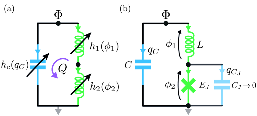
Figure 10: (a) A circuit containing two nonlinear inductive elements and a nonlinear capacitive element. Potential singularities arise in obtaining a Hamiltonian description starting with second-order Lagrangians with only flux-node/loop-charge variables. (b) A particular instance of the singular circuit in (a), studied in Ref. [84]. A Josephson junction with a capacitor $C_{J}\ll C$ is sometimes approximated by an open circuit ($C_{J}\rightarrow 0$) [84, 85].

Following the steps above, we compute the kernel of the $\operatorname{\mathsf{F}}$ matrix, where the elements are ordered such that the projectors are written as

$$\mathsf{P}^{\mathcal{C}}=\begin{pmatrix}0&0&0\\ 0&0&0\\ 0&0&1\end{pmatrix}\qquad\mathrm{and}\quad\mathsf{P}^{\mathcal{L}}=\begin{pmatrix}1&0&0\\ 0&1&0\\ 0&0&0\end{pmatrix}\,,$$ (134)

which provides us with the two-form matrix

$$[\omega_{\alpha\beta}]=\operatorname{\mathsf{K}}^{T}\operatorname{\mathsf{E}}_{2B}\operatorname{\mathsf{K}}=\begin{pmatrix}0&1&1\\ -1&0&0\\ -1&0&0\end{pmatrix},$$ (135)

with the ordering $Q$, $\phi_{1}$ and $\phi_{2}$.

Observe that we could have obtained the same result writing directly the Kirchhoff’s constraints in differential form

$$\begin{aligned} {\mathrm{d}}Q&={\mathrm{d}}q_{C}=-{\mathrm{d}}q_{1}=-{\mathrm{d}}q_{2}\\ {\mathrm{d}}\Phi&={\mathrm{d}}\phi_{C}={\mathrm{d}}\phi_{1}+{\mathrm{d}}\phi_{2},\end{aligned}$$

to compute $\omega={\mathrm{d}}Q\wedge({\mathrm{d}}\phi_{1}+{\mathrm{d}}\phi_{2})$, from which one can read the matrix $\omega_{\alpha\beta}$; recall the $2$ factor in the definition of the matrix with respect to the two-form expression. The single zero mode is

$$\mathbf{W}=\begin{pmatrix}0\\ 1\\ -1\end{pmatrix}.$$ (136)

The corresponding constraint function, $\mathbf{W}(H)=W(\Phi_{1},\Phi_{2})$, is

$$W(\phi_{1},\phi_{2}) =\frac{\partial H}{\partial\phi_{1}}-\frac{\partial H}{\partial\phi_{2}}$$ (137a)

$$=h_{1}^{\prime}(\phi_{1})-h_{2}^{\prime}(\phi_{2})=0\,,$$ (137b)

since the Hamiltonian in terms of the loop-charge and the node-fluxes is $H(Q,\phi_{1},\phi_{2})=h_{1}(\phi_{1})+h_{2}(\phi_{2})+h_{3}(Q)$.

This constraint is a useful example to better understand a type of constraints that arise from the formalism. Namely, it is in this case simply the condition that the current through both inductors has to be the same. This contrasts with the constraints in the example of F.2, that reflected the fact that there can be a nondynamical current through the capacitors, for instance.

We shall use this example to illustrate obstructions to a Hamiltonian description due to the interplay of energy functions and topology. To do so we have to examine the process of reduction by the dynamical constraint (137b) in more detail.

From the structure of the initial manifold of branch variables and from the first reduction being just Kirchhoff, we know that the three dimensional state manifold is $\mathbb{R}^{3-k}\times\left(S^{1}\right)^{k}$, i.e. $\mathbb{R}^{3}$, $\mathbb{R}^{2}\times S^{1}$, $\mathbb{R}\times\left(S^{1}\right)^{2}$ or $\left(S^{1}\right)^{3}$. We shall only consider the first two, that correspond classically to an extended ($\mathbb{R}$) variable for the loop charge and for the branch flux of one of the inductors (the linear one in the detailed analysis that follows) and a compact ($S^{1}$) variable for the other branch flux (the Josephson junction in the particularization below). In all cases, because the only constraints to this point were Kirchhoff, the total manifold is a product of the charge and fluxes submanifolds. Thus the dynamical constraint of eq. (137b) is an implicit definition of a curve in the two dimensional fluxes manifold: we are systematically assuming that the branch energy functions are smooth, and therefore so is $W(\phi_{1},\phi_{2})$ in Eq. (137), so by the implicit function theorem at all points except at flux energy extrema there will local expressions of one variable in terms of the other. If there is only one connected component of the constraint we can solve it parametrically, and we will have a description of the reduced two dimensional dynamical manifold. The remaining task is to determine the restricted two-form, and to check whether it is symplectic or not.

If we take $h_{1}(\phi_{1})=\phi_{1}^{2}/2L$ we can make a stronger assertion. As $h_{1}^{\prime\prime}$ never vanishes in this case, we can solve $\phi_{1}$ in terms of $\phi_{2}$, so we have an explicit expression for the curve satisfying the constraint, and $\phi_{2}$ can be used to describe the reduced two dimensional manifold of interest, with coordinates $(Q,\phi_{2})$. Explicitly, we can solve Eq. (137b) as

$$\phi_{1}=Lh^{\prime}_{2}(\phi_{2})\,,$$ (138)

and the reduced elements for the equations of motion are

$$\omega =\left[1+Lh_{2}^{\prime\prime}(\phi_{2})\right]\,{\mathrm{d}}Q\wedge{\mathrm{d}}\phi_{2}\,,$$ (139a)

$$H =h_{c}(Q)+h_{2}(\phi_{2})+\frac{L}{2}\left[h_{2}^{\prime}(\phi_{2})\right]^{2}\,.$$ (139b)

The equations of motion,

$$\left[1+Lh_{2}^{\prime\prime}(\phi_{2})\right]\dot{\phi}_{2} =h^{\prime}_{c}(Q)$$ (140)

$$\dot{Q} =-h_{2}^{\prime}(\phi_{2})$$

are a two-dimensional autonomous dynamical system, for which an integrating factor always exists [112], and one readily computes the first integral

$$E(Q,\phi_{2})=h_{c}(Q)+h_{2}(\phi_{2})+\frac{L}{2}\left[h_{2}^{\prime}(\phi_{2})\right]^{2}\,.$$ (141)

The level sets of this first integral are the trajectories in phase space $(\phi_{2},Q)$ of the solutions of the dynamical system (140). Therefore, there exists a classically equivalent Hamiltonian system with canonical Poisson bracket, such that the equations of motion are

$$\frac{{\mathrm{d}}\phi_{2}}{{\mathrm{d}}\tau} =\frac{\partial E}{\partial Q}=h_{c}^{\prime}(Q)\,,$$ (142a)

$$\frac{{\mathrm{d}}Q}{{\mathrm{d}}\tau} =-\frac{\partial E}{\partial\phi_{2}}=-h_{2}^{\prime}(\phi_{2})\left[1+Lh_{2}^{\prime\prime}(\phi_{2})\right]\,.$$ (142b)

We now have to take stock of this process. The strong statement is that the classical dynamics of the system has been written in Hamiltonian form, as shown in Eqs. (142). Nonetheless, there are subtleties to be considered. First and foremost, systematic reduction has taken us to Eqs. (139b). For $\omega$ in Eq. (139a) to be a symplectic form we require that it be nondegenerate. However, it will be degenerate if there are lines for which $1+Lh^{\prime\prime}_{2}(\phi_{2})=0$. The integrating factor resolves that classical singularity if it exists. The manifold described by coordinates $\phi_{2}$ and $Q$ does admit a canonical symplectic form, and the level sets of $E(Q,\phi_{2})$ are the phase space portrait. Even so, in many cases we do not simply want a Hamiltonian description, but rather a Hamiltonian description in terms of some preferred variables, and that is a completely different issue.

G.1.1 Singularities and otherwise

As stated above, for the case $h_{1}(\phi_{1})=\phi_{1}^{2}/2L$ and smoothness conditions we have a Hamiltonian description as in Eqs. (142), in terms of the loop charge $Q$ and the branch flux of the possibly nonlinear inductor $\phi_{2}$. However, in most cases of interest we would rather have a Hamiltonian description in terms of the total flux $\Phi=\phi_{1}+\phi_{2}$. As $\phi_{1}$ has been solved in terms of $\phi_{2}$, we have the relation $\Phi=\phi_{2}+Lh^{\prime}_{2}(\phi_{2})$, which slaves the evolution of $\Phi$ to $\phi_{2}$. However, if we want a description exclusively in terms of $\Phi$ this relation has to be inverted. The invertibility condition, given the smoothness of the energy functions, is $1+Lh_{2}^{\prime\prime}(\phi_{2})\neq 0$ in the range of $\phi_{2}$. i.e. monotony. Notice that this means that the two-form $\omega$ in Eq. (139a) is nondegenerate. In that case it is readily seen that eqs. (140) are equivalent to the Hamiltonian equations

$$\dot{\Phi} =h_{c}^{\prime}(Q)\,,$$

$$\dot{Q} =-V^{\prime}(\Phi)\,,$$ (143)

$$V(\Phi) =h_{2}\left[\phi_{2}(\Phi)\right]+\frac{L}{2}\left\{h_{2}^{\prime}\left[\phi_{2}(\Phi)\right]\right\}^{2}\,,$$

where $V(\Phi)$ is the energy for the equivalent inductor. We can recognize this result from Eqs. (139), with the observation that $\omega={\mathrm{d}}Q\wedge{\mathrm{d}}\Phi$.

Consider now what happens if the invertibility condition is not satisfied. Formally, inspecting Eqs. (G.1.1), we see that the evolution is Hamiltonian with conjugate $\Phi$ and $Q$, and an effective potential that has to be expressed parameterically. Much has been made of the fact that this effective potential is multibranched as a function of $\Phi$ if the invertibility condition does not hold. However, the classical motion is completely deterministic, and the phase portrait is unequivocal. Even so, the quantization of a system described parametrically deserves further investigation. We shall now give concrete examples of invertible and noninvertible situations, restricting the analysis always to the classical models.

G.1.2 Case 1: Direct reduction with two linear inductors

We now consider that the two inductors are linear, such that $h_{i}(\phi_{i})=\phi^{2}_{i}/2L_{i}$. Then the constraint can be solved, and we coordinatize the constrained surface as

$$\phi_{1} =\frac{L_{1}}{L_{1}+L_{2}}\Phi\,,$$ (144a)

$$\phi_{2} =\frac{L_{2}}{L_{1}+L_{2}}\Phi\,,$$ (144b)

so the equations of motion for $Q$ and $\Phi$ are derived from the first order Lagrangian

$$L=Q\dot{\Phi}-h_{3}(Q)-\frac{\Phi^{2}}{2(L_{1}+L_{2})}\,.$$ (145)

Naturally, this procedure has provided us with the standard reduction of series linear inductors.

To focus our mind for what follows, let us rephrase what we have done here: we have applied our procedure and obtained and effective Hamiltonian in a reduced phase space. The standard reduction formulae for linear inductors and capacitors are exactly that, a recipe for the construction of effective energy functions in fewer variables, and flow immediately from the formalism.

G.1.3 Case 2: Direct reduction with linear inductor and Josephson junction

As we have stated repeatedly, the formalism we propose here encompasses the traditional approaches to circuit analysis. Thus, the dynamical constraints of the form $\mathbf{W}(H)=0$ for zero vectors of the two-form will be readily understood in many cases as flowing from current or energy conservation. The same can be said of a dual method for obtaining Hamiltonian systems, the Dirac-Bergmann [84]. Therefore the issue of invertibility of the function that expresses the total flux $\Phi$ as a function of a parameter has already been addressed in the literature [84, 85]. The idea of regularization to start from a non-defective quadratic Lagrangian has also been put forward in this regard [84], with special emphasis on the derivation of an effective Lagrangian both under invertibility or in its absence.

For concreteness let us set the first inductor to be linear ($h_{1}(\phi_{1})=\phi_{1}^{2}/2L$) and the second one a Josephson junction with energy function $h_{2}(\phi_{2})=-E_{J}\cos(2\pi\phi_{2}/\Phi_{0})$, where $\Phi_{0}$ the standard quantum of flux, see Fig. 10(b), where the limit of $C_{J}\rightarrow 0$ has been taken before the analysis. In order to ease comparison with previous literature, we perform a standard transformation of the flux and charge variables to phase and Cooper-pair number variables, respectively, i.e., $n=Q/2e$, and $\varphi_{\alpha}=2\pi\phi_{\alpha}/\Phi_{0}$ , a transformation that is symplectic if one sets $\hbar=1$. The classical Lagrangian reads now

$$L =\hbar n(\dot{\varphi}_{1}+\dot{\varphi}_{2})-H(n,\boldsymbol{\varphi}),$$ (146)

$$H(n,\boldsymbol{\varphi}) =4E_{C}n^{2}-\frac{E_{L}}{2}\varphi_{1}^{2}-E_{J}\cos(\varphi_{2}),$$ (147)

with $E_{C}=(e)^{2}/2C$ and $E_{L}=(\Phi_{0}/2\pi)^{2}/L$. Applying again the zero-mode vector to the energy term, we solve $\varphi_{1}$ from the constraint as

$$\varphi_{1}=\beta\sin\left(\varphi_{2}\right),$$ (148)

where $\beta=L_{1}E_{J}(2\pi/\Phi_{0})^{2}=E_{J}/E_{L}$, always assumed positive in what follows. The total phase (at the capacitor), $\varphi=\Phi/\Phi_{0}=\varphi_{1}+\varphi_{2}$, is expressed after the reduction as

$$\varphi=\varphi_{2}+\beta\sin\left(\varphi_{2}\right)\,.$$ (149)

We can only invert this function $\varphi(\varphi_{2})$ if

$$\beta<1\,.$$ (150)

In this particular case, the Lagrangian in Eq. (146) becomes [84]

$$L=\hbar n\dot{\varphi}-H(n,\boldsymbol{\varphi}(\varphi)),$$ (151)

amenable to quantization, with the only caveats arising for compact $\varphi_{2}$, as inequivalent quantizations will appear [93, 94, 113]. In other words one must then consider the possibility of a gate charge parameter.

G.1.4 Multivaluedness and singularity of case 2

In spite of or because of the issues with the regime $\beta\geq 1$, that we shall now examine, it has picqued the curiosity of researchers [84, 85], and the connection to a regularized model is under active discussion. Now we study this regime intrisically, i.e. without connection to a regularized circuit.

We shall consider the two cases of $\varphi_{2}$ being: i) an extended variable ($\varphi_{2}\in\mathbb{R}$), and ii) a compact variable ($\varphi_{2}\in[0,2\pi)$ for definiteness). Observe that the total flux $\varphi$ inherits this extended or compact characteristic, although not its range.

We restate the system of Eqs. (140) for the aforementioned elements:

$$\hbar\left[1+\beta\cos\left(\varphi_{2}\right)\right]\dot{\varphi}_{2} =h_{3}^{\prime}(n)=8E_{C}n,$$ (152a)

$$\hbar\dot{n} =E_{J}\sin\left(\varphi_{2}\right).$$ (152b)

This system has a first integral

$$E_{1}=4E_{C}n^{2}-E_{J}\left[\cos\varphi_{2}+\frac{\beta}{4}\cos(2\varphi_{2})\right]\,.$$ (153)

This first integral is periodic in $\varphi_{2}$ with period $2\pi$, for the extended case. The extrema in the interval $[0,2\pi)$ are at 0, $\varphi_{*}$ (the solution of $1+\beta\cos\varphi_{2}=0$ in the interval $(\pi/2,\pi)$), $\pi$, and $2\pi-\varphi_{*}$, when $\beta>1$. $\varphi_{2}=0$ is always a minimum of the potential. However, $\varphi_{2}=\pi$ is a maximum when $\beta<1$ and becomes a minimum for $\beta>1$. $\varphi_{*}$ and $2\pi-\varphi_{*}$ enter the stage only for $\beta>1$, and they are maxima in that case. The parameter $\beta$ is a classical bifurcation parameter.

For later use, we study $\varphi_{*}$ as a function of $\beta$. Clearly, $\varphi_{*}(1)=\pi$, and $\varphi_{*}\to\pi/2$ as $\beta\to\infty$. One readily computes

$$\frac{{\mathrm{d}}\varphi_{*}}{{\mathrm{d}}\beta}=\frac{-1}{\beta\sqrt{\beta^{2}-1}}\,.$$ (154)

Notice that $\varphi_{*}$ is a monotonous decreasing function of $\beta$. Direct computation also shows that close to $\beta=1$ one has $\varphi_{*}=\pi-\sqrt{2(\beta-1)}+O\left[\left(\beta-1\right)^{2}\right]$. Consider now $\varphi_{2}$ compact with support in $[0,2\pi)$. The extrema for $\varphi(\varphi_{2})=\varphi_{2}+\beta\sin(\varphi_{2})$ will be reached either at the endpoints of the interval for $\varphi_{2}$ or at the solutions of $1+\beta\cos(\varphi_{2})=0$, if they exist. Thus, for $\beta<1$ the range of $\varphi$ will also be $(0,2\pi)$. On the other hand, for $\beta\geq 1$ we have to assess $\varphi(\varphi_{*})=\varphi_{*}+\sqrt{\beta^{2}-1}$ and $\varphi(2\pi-\varphi_{*})=2\pi-\varphi_{*}-\sqrt{\beta^{2}-1}$. For values of $\beta$ slightly larger than 1, the range of $\varphi$ will be again $(0,2\pi)$, until a critical value $\beta_{c}\approx 4.6033$ is reached, such that $2\pi=\varphi_{*}(\beta_{c})+\sqrt{\beta_{c}^{2}-1}$. From that point on, the range of $\varphi$ will be $(\varphi(2\pi-\varphi_{*}),\varphi(\varphi_{*}))$. Asymptotically, $(-\beta,\beta)$ for large $\beta$.

Let us examine qualitatively the system from the perspective of the total phase $\varphi$. The current is always bounded, by Eq. (152b), and as $\dot{\varphi}=8E_{C}n$ the evolution is not singular. The issue is that if $\varphi_{2}$ reaches $\varphi_{*}$ or $2\pi-\varphi_{*}$ (modulo $2\pi$ in the extended case) the velocity of $\varphi_{2}$ is required to be infinite, to compensate that $\dot{\varphi}=8E_{C}n/\hbar$ is finite. This corresponds to infinite voltage drops in both inductor branches, even though the total voltage drop is finite. We can describe the motion with a parametric expression for potential energy and the total phase,

$$\varphi =\sigma+\beta\sin\sigma\,,$$

$$V =-E_{J}\left[\cos\sigma+\frac{\beta}{4}\cos(2\sigma)\right]\,.$$ (155)

There has been previous discussion about this kind of system and its quantization (for instance by Shapere and Wilczeck [114]), and we defer to future work this aspect of the model.

The parametric presentation of the potential allows a qualitative analysis for small and large $\beta$, that will guide that quantum analysis. Small $\beta$ corresponds to the inductance of the linear inductor going to 0, which corresponds to there being no phase drop, and the system is simply the capacitor and the nonlinear inductor. This physical description matches the limit of the effective potential. Large $\beta$, physically, means that the linear inductor has no current flowing through it, so the system is no longer dynamical, and all the energy will be the electrostatic energy of the capacitor. I.e., the physical expectation is that the effective potential will be flat in that limit. Consider the case of compact $\varphi_{2}$. Then so is $\varphi$, with range (in the large $\beta$ case) $(\varphi(2\pi-\varphi_{*}),\varphi(\varphi_{*}))$. Therefore $\varphi/\beta$ is uniformly bounded as $\beta\to\infty$, $|\varphi|/\beta<1+\pi/\beta$. Inversion is not possible in the full range. However, given a large fixed $\Phi$, for all $|\varphi|<\Phi$ , as $\beta\to\infty$, inversion is possible, $\sigma=\varphi/\beta+O(\beta^{-2})$. It follows that

$$V\approx-E_{J}\left[1+\frac{\beta}{4}-\frac{1}{2}\frac{\varphi^{2}}{\beta}+O(\beta^{-2})\right]\,,$$ (156)

effectively flat as expected, for a fixed range $(-\Phi,\Phi)$. For extended $\varphi_{2}$, the argument is slightly different. There will exist an integer $N$ such that $\sigma=2\pi N+\zeta$, with $\zeta$ in $[0,2\pi)$. Then $\zeta$ will be small, $\zeta=\left(\varphi-2\pi/N\right)/\beta+O(\beta^{-2})$, and applying the same argument as before we see again that $V$ flattens out as $\beta\to\infty$, matching the physical argument.

It is important to observe that in the large $\beta$ limit the variable $\varphi$ effectively decompactifies, if it started out with a finite range, at the same time that its potential flattens out away from the boundaries. Therefore, when it comes to quantization, where the behaviour of compact variables is radically different from extended ones, we will in both cases have an approximate continuum spectrum. This argument can be presented in an alternative way: in this large $\beta$ limit, all the energy is in the capacitor, due to its charge, and that charge need no longer be discretized.

G.1.5 Regularized problem of case 2

In order to have a better handle of the quantization of these circuits, Rymarz and DiVincenzo [84] start their analysis with the regularized classical circuit Hamiltonian (obtained from Fig. 10(b) with finite Josephson capacitance $C_{J}$). After canonical quantization, they carry out a Born–Oppenheimer analysis as $C_{J}\rightarrow 0$ with the expectation that there will be a clear separation of scales.

Using the same redefinitions as above and the notation in the corresponding figure, and following our method (observe that here the standard flux-node analysis [27] provides us with the same result), one obtains the Hamiltonian

$$H=4E_{C}(n_{C}^{2}+rn_{C_{J}}^{2})+\frac{E_{J}}{2\beta}(\varphi_{C}-\varphi_{2})^{2}-E_{J}\cos{\varphi_{2}},$$ (157)

with the additional parameter $r=C/C_{J}$, as well as the canonical brackets $\{\varphi_{C},n_{C}\}=\{\varphi_{2},n_{C_{J}}\}=1$. Recall the definition $\beta=E_{J}/E_{L}$. The main goal in the analysis of [84] is its quantization and separation of scales. Here we shall just analyze it classically, including adiabatic expansions, i.e. classical separation of scales.

	$0<r<\infty$	$r\rightarrow\infty$
$0<\beta<\infty$	2 d.o.f., $H$ in Eq. (157)	1 d.o.f. $H$ in (147)
$\beta\rightarrow 0$	1 d.o.f. ($H=4E_{C}rn_{a}^{2}/(r+1)-E_{J}\cos\varphi_{a}$)	1. d.o.f ($H=4E_{C}n_{a}^{2}-E_{J}\cos\varphi_{a}$)
$\beta\rightarrow\infty$	2 d.o.f. (1 free) ($H=4E_{C}n_{C}^{2}+\left[E_{C}rn_{C_{J}}^{2}-E_{J}\cos{\varphi_{2}}\right]$)	1 (free) d.o.f. ($H=4E_{C}n_{C}^{2}$)

Table 1: Summary table for the different classical Hamiltonian models of circuit in Fig. 10(b). We stress the number of effective degrees of freedom, and the appearance of a free particle.

In particular, we want to address the exchangeability of the limits $\beta\to\infty$ or $\beta\to 0$, on one hand, and $r\to\infty$ on the other. Physically, as $\beta\to 0$ the argument above holds: there will be no phase drop in the strict limit through the linear inductor. Therefore the circuit will be equivalent to that of a JJ with a parallel total equivalent capacitance $\tilde{C}=C+C_{J}$, independent of the value of $C_{J}$. Let us now check this intuition against the equations of motion, after a symplectic change of variables

$$\begin{aligned} n_{C}&=\frac{1}{2}n_{a}+n_{b},\qquad n_{C_{J}}=\frac{1}{2}n_{a}-n_{b},\\ \varphi_{C}&=\varphi_{a}+\frac{1}{2}\varphi_{b},\qquad\varphi_{2}=\varphi_{a}-\frac{1}{2}\varphi_{b},\end{aligned}$$ (158)

with obvious notation, $\varphi_{a}$ and $n_{a}$ being a conjugate pair and $\varphi_{b}$ and $n_{b}$ a second one, such that the mass matrix is no longer diagonal,

$$H= \,E_{C}\left[4(1+r)n_{b}^{2}+4(1-r)n_{a}n_{b}+(1+r)n_{a}^{2}\right]$$

$$+\frac{E_{J}}{2\beta}\varphi_{b}^{2}-E_{J}\cos\left(\varphi_{a}-\varphi_{b}/2\right)\,.$$ (159)

This means that the only equation of motion in which the $\beta$ parameter appears is $\dot{n}_{b}=-\partial H/\partial\varphi_{b}$, and we conclude that

$$\varphi_{b}=\beta\left[\frac{1}{2}\sin\left(\varphi_{a}-\frac{\varphi_{b}}{2}\right)-\frac{1}{E_{J}}\dot{n}_{b}\right]\,.$$ (160)

Adiabatic elimination to first order is therefore $\varphi_{b}=0$, and for consistency $\dot{\varphi}_{b}=\partial H/\partial n_{b}=0$ that fixes $n_{b}=(r-1)n_{a}/2(r+1)$, providing us with a reduced system, i.e. of one fewer degree of freedom, with total charge number $n$ conjugate to the phase of the JJ, and potential energy that of the JJ. Explicitly, $H=4E_{C}rn_{a}^{2}/(r+1)-E_{J}\cos\varphi_{a}$, which corresponds to the equivalent capacitor with total capacity $C+C_{J}$. Furthermore, notice that this system of equations is amenable to a systematic expansion in $\beta$, giving rise perturbatively to a reduced dynamics. Explicitly, in a $\beta$ expansion of the form $\varphi_{j}=\sum_{m=0}^{\infty}\beta^{m}\varphi_{j}^{(m)}$, with $j$ being either $a$ or $b$, and correspondingly for $n_{j}$, order by order $\varphi_{b}^{(m)}$ and $n_{b}^{(m)}$ are completely determined by $\left\{\varphi_{a}^{(m^{\prime})}\right\}$ and $\left\{n_{a}^{(m^{\prime})}\right\}$, with $m^{\prime}\leq m$. This result is independent of the value of $r$, so the limit $r\to\infty$ is immediate.

Now we start from the limit $r\to\infty$ first with Hamiltonian (157). From the equations of motion we see that $n_{2}$ has to be zero. Rather that direct substitution in the Hamiltonian, one should stick to the equations of motion to carry out this approximation. Thus $n_{2}=0$ demands for consistency $\dot{n}_{2}=0$, whence $\varphi_{C}=\varphi_{2}+\beta\sin\varphi_{2}$, and the approximate equations of motion are exactly the system we analyzed above. Again the limit is singular in that there is only one remaining degree of freedom. It has to be pointed out that this appears to be in contradiction with the result in [84], where it was suggested that in the quantum mechanical context the effective potential in the limit $r\to\infty$ is always zero. Clearly the issue deserves further investigation, that we defer to future work.

Finally we check again the limit $\beta\to\infty$, now in this regularized model. The physical intuition is as above, that there will be no current through the linear inductor. Consequently, we shall have electrostatic energy in the $C$ capacitor, and a dynamical system composed exclusively of the JJ and the regularization capacitor $C_{J}$. This intuition is read off directly from the equations of motion, in fact, since one sees the requirement for $\dot{n}_{C}=0$ in the limit, separating off the $n_{2}$ and $\varphi_{2}$ variables. However there are two degrees of freedom, one of which is a free particle.

As $\beta\to\infty$ gives us two degrees of freedom and $r\to\infty$ one, we now check whether these limits commute. Starting from the $\beta\to\infty$ limit Hamiltonian, $H=4E_{C}n_{C}^{2}+\left[E_{C}rn_{C_{J}}^{2}-E_{J}\cos{\varphi_{2}}\right]$, and considering $r\to\infty$, $n_{{C_{J}}}$ must be frozen to zero and $\varphi_{2}$ has no dynamics, thus having an effective Hamiltonian $H=4E_{C}n_{C}^{2}$. Interchanging the order, we begin with $H=4E_{C}n^{2}-E_{J}\varphi_{1}^{2}/2\beta-E_{J}\cos\varphi_{2}$ and take $\beta\to\infty$, as we analyzed above, with the effective potential flattening out and leaving us again with one free particle.

In these classical analyses the issue of compactness or otherwise of the variables has not played a crucial role. On the other hand, were we to fully address quantization (which we defer to later work), it would be crucial to have this aspect in mind. For instance, even if the effective potential for a compact variable were flat, the corresponding spectrum would be discrete. On the other hand, in a system with two degrees of freedom with an extended variable and a bounded potential in some direction that partakes of this extended aspect, the spectrum will be continuous. The models we have been looking at here are debated currently as extremely idealized ones for simple circuits in which a superconducting island appears. In this situation, the assumption of a compact phase ($\varphi_{2}\in S^{1}$) matches the experimental data, e.g., the discrete spectra, on charge qubits in any coupling regime, including the Cooper-Pair Box ($E_{J}\sim E_{C}$) and transmon regimes ($E_{J}\gg E_{C}$). Thus, even deferring to future work the detailed study of quantization under regularization, we point out that the classical analysis we put forward here, together with general considerations on the quantum models that flow from it, is in accordance with experiments [115, 116].

G.2 Singular multi-junction branches

In this section we will apply our method to reproduce, contextualize, and expand on the results presented in Ref. [85], as an example of the versatility of this formalism. The objective of Miano et al. is to provide a method to identify minima in a superconducting circuit context and thus allow for an expansion around those minima. Miano et al. consider a very particular class of circuits, in which there exists a loop of Josephson junctions and inductors. They want to study low energy physics, in the sense that they want to characterize the minima of the potential energy, that is a function of the node fluxes, as they assume that a node-flux description of the larger circuit is not defective. To do so, they ask what current intensity is being injected into the inductive loop at each node between inductive elements in a general state, and then they observe that in a minimum of inductive energy, and thus in a possible steady state, this current injection must be zero. They arrive to that result by a Tellegen like argument. They next study the equivalent inductive element that would describe the same low energy phenomena, if the adjoining capacitors are negligible.

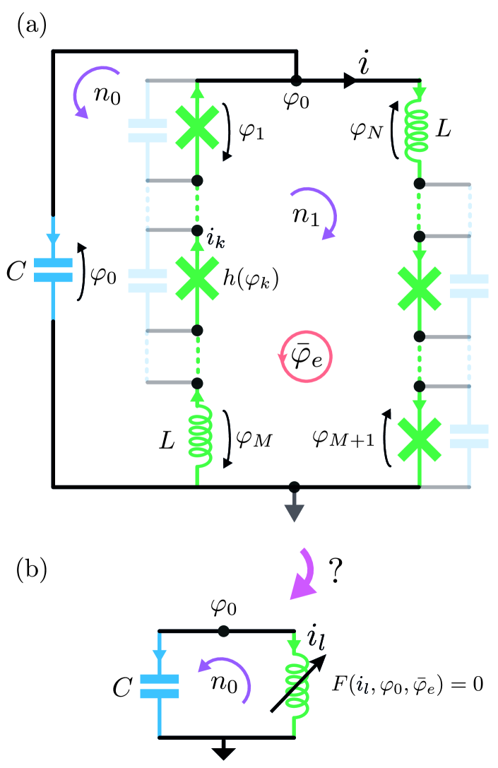
Figure 11: A nonlinear dipole, investigated in Ref. [85], is constructed using a series of Josephson junctions and linear inductors. A persistent inquiry in the literature revolves around the challenge of mapping the response of a multi-dipole problem to a single element.

G.2.1 Effective Hamiltonian

The main objective of Miano et al. is the study of the effective Hamiltonian for a configuration included in those presented in Fig. 11. We shall compute that effective Hamiltonian straightforwardly using our method. In particular, we will make use of the differential form presentation rather than the equivalent matricial one we have insisted on above, as it is more convenient for the treatment of general models. We intend this material to be pedagogical, so we shall be very explicit in the construction. It should be pointed out that, as the system consists purely of ideal reactances, the result can be derived as a direct application of Kirchhoff’s laws. However, we contend that the generality and systematics of our proposal are useful in identifying correctly the relevant quantities. In particular, the goal of [85] is to evidence that the full system is well described by

$$H=4E_{C}n_{0}^{2}+U_{\mathrm{eff}}(\varphi_{0},\varphi_{e})\,,$$ (161)

where $\varphi_{0}$ is conjugate to $n_{0}$ and dynamical, and $\varphi_{e}$ a (constant) external flux controls the inner current.

In a nutshell, we have three effective branches, the capacitor one and two inductive series, that we shall refer to respectively as the outer and inner edges of the inductive loop. We shall use $n_{0}$ and $n_{1}$ charge number and $\left\{\varphi_{k}\right\}_{k=0}^{N+1}$ branch phase variables. From the figure, we see that $\varphi_{0}$ is also the top node phase. The energy function is simply

$$H\left(n_{0},\left\{\varphi_{k}\right\}_{k=0}^{N+1}\right)=h_{c}(n_{0})+\sum_{k=1}^{N+1}h_{k}(\varphi_{k})\,.$$ (162)

Prima facie, it seems that neither $\varphi_{0}$ nor $\varphi_{e}$ play a role. However, we have yet to determine all the constraints. To do so, we observe that the KVL forces us to have

$${\mathrm{d}}\varphi_{e} =\sum_{k=1}^{N+1}{\mathrm{d}}\varphi_{k}\,,$$ (163a)

$${\mathrm{d}}\varphi_{0} =-\sum_{k=1}^{M}{\mathrm{d}}\varphi_{k}$$ (163b)

$$=-{\mathrm{d}}\varphi_{e}+\sum_{k=M+1}^{N+1}{\mathrm{d}}\varphi_{k}\,.$$ (163c)

We shall make use of these in the two form, that, following our general constructions, reads

$$\omega =\frac{1}{2}{\mathrm{d}}n_{0}\wedge{\mathrm{d}}\varphi_{0}$$ (164a)

$$\,+\frac{1}{2}\sum_{k=M+1}^{N+1}{\mathrm{d}}\varphi_{k}\wedge{\mathrm{d}}n_{1}$$ (164b)

$$\,+\frac{1}{2}\sum_{k=1}^{M}{\mathrm{d}}\varphi_{k}\wedge\left({\mathrm{d}}n_{0}+{\mathrm{d}}n_{1}\right)$$ (164c)

$$={\mathrm{d}}n_{0}\wedge{\mathrm{d}}\varphi_{0}+\frac{1}{2}{\mathrm{d}}\varphi_{e}\wedge{\mathrm{d}}n_{1}\,.$$ (164d)

For simplicity we have set $\hbar=1$. The first line (164a) corresponds to the capacitive branch, the second one (164b) to the outer inductive branch, and finally the third one (164c) to the inner inductive branch.

As was to be expected, there can be only two degrees of freedom, and that just if $\varphi_{e}$ is time dependent. Otherwise only $n_{0}$ and its conjugate will be dynamical, and we have to carry out symplectic reduction to make that fact explicit. For definiteness we shall only consider fixed $\varphi_{e}$, so we have the simple two-form $\omega={\mathrm{d}}n_{0}\wedge{\mathrm{d}}\varphi_{0}$.

It is clear that this two form is defective: we have $N+2$ branches in total, so before imposing Kirchhoff’s laws we had $2N+4$ branch variables, and after imposing Kirchhoff these must be reduced to $N+2$. These are in fact the the two charges and $N$ phases. One of the charges, $n_{1}$, is directly eliminated, as it appears neither in the two-form nor in the Hamiltonian, so the associated zero vector $\partial/\partial n_{1}$ is gauge. In other words, there can exist a nondynamical current around the inductive loop. If $\varphi_{e}$ were time-dependent it would drive this current $\dot{n}_{1}$. We fix it to zero, with constant $\varphi_{e}$.

Therefore, we are left with one charge, $n_{0}$, and $N$ phases. However the two form, $\omega={\mathrm{d}}n_{0}\wedge{\mathrm{d}}\varphi_{0}$, is obviously rank two. Therefore there must exist $N-1$ independent zero vectors. Now, because of Eq. (163b) we have

$$\left\langle{\mathrm{d}}\varphi_{0},\frac{\partial}{\partial\varphi_{k}}\right\rangle=-1$$ (165)

for $k\in\left\{1,\ldots,M\right\}$, and from Eq. (163c), together with ${\mathrm{d}}\varphi_{e}=0$,

$$\left\langle{\mathrm{d}}\varphi_{0},\frac{\partial}{\partial\varphi_{k}}\right\rangle=1$$ (166)

for $k\in\{M+1,\ldots,N+1\}$. Therefore we have

$$\mathbf{W}_{k}=\frac{\partial}{\partial\varphi_{k+1}}-\frac{\partial}{\partial\varphi_{k}}$$ (167)

with $k$ from $1$ to $M-1$ and from $M+1$ to $N$ are zero vectors. They are in fact independent, and they number a total of $M-1+\left(N-(M+1)+1\right)=N-1$. We have a complete independent set.

These zero vectors provide us with the consistency constraints, $\mathbf{W}_{k}(H)=0$, which are in fact current conservation constraints in this case, here

$$h^{\prime}_{k+1}(\varphi_{k+1})=h^{\prime}_{k}(\varphi_{k})$$ (168)

for $k\in\left\{1,\ldots,M-1\right\}\cup\{M+1,\ldots,N\}$. Essentially, for $k=0$ and $k=M$ there can be current extraction or injection, and therefore those nodes are missing from the sequence of Eq. (168).

Putting everything together, we have an expression for the inductive energy in terms of the $N+1$ inductive branch phases, on the one hand, 2 KVL constraint equations in which the additional $\varphi_{0}$ and $\varphi_{e}$ are introduced (raising the number of total phase variables to $N+3$), and an additional $N-1$ current conservation constraints. All in all, $N+3$ phases and $1+2+N-1=N+2$ relations, which, after elimination of the $N+1$ loop inductive branch phases, leaves us with an expression of the inductive energy in terms of $\varphi_{0}$ and $\varphi_{e}$. In other words, this system will always present with an inductive energy depending on those variables. The only caveat to provide an explicit form is that it might well be the case, as we will now show, that it is not possible to reexpress all $\varphi_{k}$ from 1 to $N+1$ in terms of $\varphi_{0}$ and $\varphi_{e}$. At any rate, if not we would still have the inductive energy as a function of $\varphi_{0}$ and $\varphi_{e}$, albeit in implicit form.

G.2.2 Example

Let us apply the previous computation to the case where all the inductive elements, in both the inner and the outer edges of the loop, are either linear inductances or JJ inductances. I.e. where all the inductive energies $h_{k}$ are of either the form

$$h_{k}(\varphi_{k})=\frac{E_{k}}{2}\varphi_{k}^{2}$$ (169)

or

$$h_{k}(\varphi_{k})=-E_{k}\cos(\varphi_{k})\,.$$ (170)

If all the inductors in one of the edges of the loop are linear, they can all be parameterized by $\varphi_{\mathrm{linedge}}=\sum_{k\in\mathrm{edge}}\varphi_{k}$ as $\varphi_{k}=E_{\mathrm{linedge}}\varphi/E_{k}$, with $E_{\mathrm{linedge}}=\left(\sum_{k\in\mathrm{edge}}E_{k}^{-1}\right)^{-1}$, and we have the standard equivalent inductor of the linear case. Let us therefore assume that there is at least one JJ inductance in the edge. Without loss of generality, let the JJ inductance with the smallest $E$ coefficient amongst the JJ inductances be the first one of the edge of the loop. We shall first take the inner edge for definiteness, so $E_{1}$ is the smallest energy coefficient of all the JJ inductances on that loop. Define $\beta_{k}=E_{1}/E_{k}$ for all inductors on the inner edge. Then the constraint equations (168) are either

$$\varphi_{k}=\beta_{k}\sin\varphi_{1}\,,$$ (171)

for the linear inductances of the edge, or

$$\varphi_{k}=\arcsin{\left(\beta_{k}\sin\varphi_{1}\right)}$$ (172)

for the JJ inductances. Observe that for all JJ inductances $\beta_{k}\leq 1$ by construction, so Eq. (172) can be followed consistently. At any rate, we have an explicit parameterization of the solution of the constraint equations, $\varphi_{k}=f_{k}(\varphi_{1})$, for the inner edges. In exactly the same manner we also have $\varphi_{k}=f_{k}(\varphi_{M+1})$ for the outer edge.

Now we express the final variables $\varphi_{0}$ and $\varphi_{e}$ in terms of the two parameters $\varphi_{1}$ and $\varphi_{M+1}$,

$$\varphi_{0} =-\sum_{k=1}^{M}f_{k}(\varphi_{1})\,,$$ (173a)

$$\varphi_{e} =-\varphi_{0}+\sum_{k=M+1}^{N+1}f_{k}(\varphi_{M+1})\,.$$ (173b)

The relevant question at this point is whether these relations can be inverted, so that we can express $\varphi_{1}=g_{1}(\varphi_{0})$ and $\varphi_{M+1}=g_{2}(\varphi_{0}+\varphi_{e})$. As all $f_{k}$ functions are smooth, the question is whether the sums in eqs. (173) are monotonous functions of $\varphi_{1}$ and $\varphi_{M+1}$. In other words, we have to investigate whether the equations

$$\sum_{k=1}^{M}f_{k}^{\prime}(\sigma_{1}) =0\qquad\mathrm{and}$$

$$\sum_{k=M+1}^{N+1}f_{k}^{\prime}(\sigma_{2}) =0$$

have roots. We defer to Ref. [85] for an analysis of some examples.

G.2.3 Stationary state and inductive loop.

In the previous G.2.1 we have addressed the construction of the principal object of interest in [85], the effective potential of an inductive dipole. Another aspect that Miano et al addressed was the identification of minima for expansions. Let us give a direct proof of their first result at this point, concerning the steady state of an inductive loop connected to a network through capacitive elements. We use an index $k$ to identify individual inductive elements in the loop, and denote branch currents (in fact, number currents, as we are normalizing charges with the Cooper pair charge, but we maintain the notation of current intensity) and branch phases as $i_{k}$ and $\varphi_{k}$. The energy function for each inductive element is $h_{k}(\varphi_{k})$. The total inductive energy of the loop is the sum of these energy functions, $U_{\mathrm{ind}}=\sum_{k}h_{k}$. In fact, a reduction of variables due to the Kirchhoff constraints in the circuits they consider is equivalent to considering node phases. We number the inductive elements sequentially, and choose the numbering of the nodes correspondingly, such that the $k$-th element connects the $k-1$-th node to the $k$-th node. The $0$th node is the reference node. Thus the branch phase of the $k$-th element, $\varphi_{k}$, equals the difference of the $k$-th and the $k-1$-th node phases, $\varphi_{k}=\phi_{k}-\phi_{k-1}$. The inductive energy of the loop is presented as a function of the node phases, $U_{\mathrm{ind}}(\boldsymbol{\phi})$.

The constitutive equation for the inductive elements is

$${i}_{k}=\frac{\partial h_{k}}{\partial{\varphi}_{k}}\,.$$ (174)

Now, by construction, ${\varphi}_{k}=\phi_{k}-\phi_{k-1}$, so

$$\frac{\partial}{\partial\phi_{k}}=-\frac{\partial}{\partial{\varphi}_{k}}+\frac{\partial}{\partial{\varphi}_{k+1}}\,.$$ (175)

Therefore,

$$\frac{\partial U_{\mathrm{ind}}}{\partial\phi_{k}}=-{i}_{k+1}+{i}_{k}=j_{k}\,,$$ (176)

where we have introduced the symbol $j_{k}$ for the current injected at the $k$-th node. This result (Eq. (5) of Ref. [85]) holds for any dynamical situation, be it a steady state or not. Even more, this holds even if the inductive loop is connected to other elements, not solely capacitors providing one loop per inductive element, as in the description by Miano et al. For instance, this holds true even if the node-flux Lagrangian is defective. The derivation here flows from the Kirchhoff constraints. In Ref. [85] it was obtained from a Tellegen type argument. As Tellegen’s global property flows from the Kirchhoff laws, and, furthermore, any one of the Kirchhoff laws together with Tellegen’s property implies the other one, these derivations are equivalent.

The next statement in the search of minima that are suitable for expansion and posterior quantization is that, in a classical stationary state, $\nabla_{\phi}U_{\mathrm{ind}}(\boldsymbol{\phi})=0$. This is not as general as the previous result. For this to hold, the only inductive elements connected to the nodes of interest must be those in the loop. Under this condition, the next result by Miano et al. is that in a stationary state the current in all branches of a purely inductive loop has to be the same. In other words, for all elements $j$, $k$ in the inductive loop in a stationary state we must have

$$h^{\prime}_{k}(\varphi_{k})=h^{\prime}_{j}(\varphi_{j})\,.$$ (177)

This more concrete result is the starting point in the analysis of Miano et al to look at an effective inductive dipole, along the lines of subsection G.2.1. Notice that (177) are in direct correspondence with (168).

References

- Jackson [1999] J. D. Jackson, Classical electrodynamics, 3rd ed. (Wiley, New York, 1999).
- Feynman et al. [2010] R. Feynman, R. Leighton, and M. Sands, The Feynman Lectures on Physics, Vol. II: Mainly Electromagnetism and Matter, new millennium ed. (Basic Books, New York, 2010).
- Caldeira and Leggett [1981] A. O. Caldeira and A. J. Leggett, Physical Review Letters 46, 211 (1981).
- Yurke and Denker [1984] B. Yurke and J. S. Denker, Physical Review A 29, 1419 (1984).
- Blais et al. [2021] A. Blais, A. L. Grimsmo, S. M. Girvin, and A. Wallraff, Review Modern Physics 93, 025005 (2021).
- Parra-Rodriguez [2021] A. Parra-Rodriguez, PhD Thesis: Canonical Quantization of Superconducting Circuits (Universidad del Pais Vasco, Leioa, 2021).
- Foster [1924] R. M. Foster, Bell Systems Technical Journal 6, 259 (1924).
- Cauer [1926] W. Cauer, Doktorarbeit: Die Verwirklichung der Wechselstrom- widerstände vorgeschriebener Frequenzabhängigkeit. (TH Berlin, Berlin, 1926).
- Cauer [1929] W. Cauer, Elektrische Nachrichtentechnik (ENT) 6, 272 (1929).
- Brune [1931] O. Brune, PhD Thesis: Synthesis of a finite two-terminal network whose driving-point impedance is a prescribed function of frequency (M.I.T., Boston, 1931).
- Tellegen [1948a] B. D. H. Tellegen, Philips Research Reports 3, 81 (1948a).
- Belevitch [1950] V. Belevitch, Electrical Communication 27, 231 (1950).
- Cauer [1954] W. Cauer, Theorie der linearen Wechselstromschaltungen, 2nd ed. (Akademie-Verlag GmbH, Berlin, 1954).
- Newcomb [1966] R. W. Newcomb, Linear Multiport Synthesis (McGraw-Hill, New York, 1966).
- Anderson and Moylan [1975] B. Anderson and P. Moylan, International Journal of Circuit Theory and Applications 3, 193 (1975).
- Wells [1938] D. A. Wells, Journal of Applied Physics 9, 312 (1938).
- Wells [1945] D. A. Wells, Journal of Applied Physics 16, 535 (1945).
- MacFarlane [1969] A. MacFarlane, Proceedings of the Institution of Electrical Engineers 116, 1453(4) (1969).
- Chua and McPherson [1974] L. Chua and J. McPherson, IEEE Transactions on Circuits and Systems 21, 277 (1974).
- Kwatny et al. [1982] H. Kwatny, F. Massimo, and L. Bahar, IEEE Transactions on Circuits and Systems 29, 220 (1982).
- Shragowitz and Gerlovin [1988] E. Shragowitz and E. Gerlovin, International Journal of Circuit Theory and Applications 16, 129 (1988).
- Bernstein and Lieberman [1989] G. Bernstein and M. Lieberman, IEEE Transactions on Circuits and Systems 36, 411 (1989).
- Maschke et al. [1995] B. Maschke, A. van der Schaft, and P. Breedveld, IEEE Transactions on Circuits and Systems I: Fundamental Theory and Applications 42, 73 (1995).
- Weiss and Mathis [1997] L. Weiss and W. Mathis, IEEE Transactions on Circuits and Systems I: Fundamental Theory and Applications 44, 843 (1997).
- Van Der Schaft [2006] A. Van Der Schaft, in Proceedings of the international congress of mathematicians, Vol. 3, Marta Sanz-Sole, Javier Soria, Juan Luis Verona, Joan Verdura, Madrid, Spain (European Mathematical Society Publishing House (EMS Ph), 2006) pp. 1339–1365.
- Van Der Schaft and Jeltsema [2014] A. Van Der Schaft and D. Jeltsema, Foundations and Trends® in Systems and Control 1, 173 (2014).
- Devoret [1995] M. H. Devoret, in Proceedings of the Les Houches Summer School, Session LXIII (Elsevier, edited by S. Reynaud, E. Giacobino, and J. Zinn-Justin, New York, 1995).
- Burkard et al. [2004] G. Burkard, R. H. Koch, and D. P. DiVincenzo, Physical Review B 69, 064503 (2004).
- Burkard [2005] G. Burkard, Physical Review B 71, 144511 (2005).
- Ulrich and Hassler [2016] J. Ulrich and F. Hassler, Physical Review B 94, 094505 (2016).
- Parra-Rodriguez and Egusquiza [2022a] A. Parra-Rodriguez and I. L. Egusquiza, Quantum 6, 681 (2022a).
- Egusquiza and Parra-Rodriguez [2022] I. L. Egusquiza and A. Parra-Rodriguez, Physical Review B 106, 024510 (2022).
- Chakravarty and Schmid [1986] S. Chakravarty and A. Schmid, Physical Review B 33, 2000 (1986).
- Yurke [1987] B. Yurke, Journal of the Optical Society of America B 4, 1551 (1987).
- Paladino et al. [2003] E. Paladino, F. Taddei, G. Giaquinta, and G. Falci, Physica E: Low-Dimensional Systems and Nanostructures 18, 39 (2003).
- Blais et al. [2004] A. Blais, R.-S. Huang, A. Wallraff, S. M. Girvin, and R. J. Schoelkopf, Physical ReviewA 69, 062320 (2004).
- Houck et al. [2008] A. A. Houck, J. A. Schreier, B. R. Johnson, J. M. Chow, J. Koch, J. M. Gambetta, D. I. Schuster, L. Frunzio, M. H. Devoret, S. M. Girvin, and R. J. Schoelkopf, Physical Review Letters 101, 080502 (2008).
- Bourassa et al. [2009] J. Bourassa, J. M. Gambetta, A. A. Abdumalikov, O. Astafiev, Y. Nakamura, and A. Blais, Physical Review A 80, 032109 (2009).
- Clerk et al. [2010] A. A. Clerk, M. H. Devoret, S. M. Girvin, F. Marquardt, and R. J. Schoelkopf, Reviews of Modern Physics 82, 1155 (2010).
- Koch et al. [2010] J. Koch, A. A. Houck, K. L. Hur, and S. M. Girvin, Physical Review A 82, 043811 (2010).
- Filipp et al. [2011] S. Filipp, M. Göppl, J. M. Fink, M. Baur, R. Bianchetti, L. Steffen, and A. Wallraff, Physical Review A 83, 063827 (2011).
- Bourassa et al. [2012] J. Bourassa, F. Beaudoin, J. M. Gambetta, and A. Blais, Physical Review A 86, 013814 (2012).
- Bergenfeldt and Samuelsson [2012] C. Bergenfeldt and P. Samuelsson, Physical Review B 85, 045446 (2012).
- Peropadre et al. [2013] B. Peropadre, J. Lindkvist, I.-C. Hoi, C. M. Wilson, J. J. Garcia-Ripoll, P. Delsing, and G. Johansson, New Journal of Physics 15, 035009 (2013).
- Nigg et al. [2012] S. E. Nigg, H. Paik, B. Vlastakis, G. Kirchmair, S. Shankar, L. Frunzio, M. H. Devoret, R. J. Schoelkopf, and S. M. Girvin, Physical Review Letters 108, 240502 (2012).
- Devoret and Schoelkopf [2013] M. Devoret and R. Schoelkopf, Science 339, 1169 (2013).
- Solgun et al. [2014] F. Solgun, D. W. Abraham, and D. P. DiVincenzo, Physical Review B 90, 134504 (2014).
- Sundaresan et al. [2015] N. M. Sundaresan, Y. Liu, D. Sadri, L. J. Szőcs, D. L. Underwood, M. Malekakhlagh, H. E. Türeci, and A. A. Houck, Physical Review X 5, 021035 (2015).
- Solgun and DiVincenzo [2015] F. Solgun and D. DiVincenzo, Annals of Physics 361, 605 (2015).
- Malekakhlagh and Türeci [2016] M. Malekakhlagh and H. E. Türeci, Physical Review A 93, 012120 (2016).
- Mortensen et al. [2016] H. L. Mortensen, K. Mølmer, and C. K. Andersen, Physical Review A 94, 053817 (2016).
- Roy and Devoret [2016] A. Roy and M. Devoret, Comptes Rendus Physique 17, 740 (2016).
- Vool and Devoret [2017] U. Vool and M. Devoret, International Journal of Circuit Theory and Applications 45, 897 (2017).
- Malekakhlagh et al. [2017] M. Malekakhlagh, A. Petrescu, and H. E. Türeci, Physical Review Letters 119, 073601 (2017).
- Roy and Devoret [2018] A. Roy and M. Devoret, Physical Review B 98, 045405 (2018).
- Parra-Rodriguez et al. [2018] A. Parra-Rodriguez, E. Rico, E. Solano, and I. L. Egusquiza, Quantum Science and Technology 3, 024012 (2018).
- Jeltsema and Van Der Schaft [2009] D. Jeltsema and A. J. Van Der Schaft, Reports on Mathematical Physics 63, 55 (2009).
- Mariantoni [2020] M. Mariantoni, arXiv:2007.08519 [class-ph] (2020).
- Parra-Rodriguez et al. [2019] A. Parra-Rodriguez, I. L. Egusquiza, D. P. DiVincenzo, and E. Solano, Physical Review B 99, 014514 (2019).
- Rymarz et al. [2021] M. Rymarz, S. Bosco, A. Ciani, and D. P. DiVincenzo, Physical Review X 11, 011032 (2021).
- Parra-Rodriguez and Egusquiza [2022b] A. Parra-Rodriguez and I. L. Egusquiza, Physical Review B 106, 054504 (2022b).
- Kerckhoff et al. [2015] J. Kerckhoff, K. Lalumière, B. J. Chapman, A. Blais, and K. W. Lehnert, Physical Review Applied 4, 034002 (2015).
- Sliwa et al. [2015] K. M. Sliwa, M. Hatridge, A. Narla, S. Shankar, L. Frunzio, R. J. Schoelkopf, and M. H. Devoret, Physical Review X 5, 041020 (2015).
- Lecocq et al. [2017] F. Lecocq, L. Ranzani, G. A. Peterson, K. Cicak, R. W. Simmonds, J. D. Teufel, and J. Aumentado, Physical Review Applied 7, 024028 (2017).
- Chapman et al. [2017] B. J. Chapman, E. I. Rosenthal, J. Kerckhoff, B. A. Moores, L. R. Vale, J. A. B. Mates, G. C. Hilton, K. Lalumière, A. Blais, and K. W. Lehnert, Physical Review X 7, 041043 (2017).
- Mahoney et al. [2017] A. C. Mahoney, J. I. Colless, S. J. Pauka, J. M. Hornibrook, J. D. Watson, G. C. Gardner, M. J. Manfra, A. C. Doherty, and D. J. Reilly, Physical Review X 7, 011007 (2017).
- Barzanjeh et al. [2017] S. Barzanjeh, M. Wulf, M. Peruzzo, M. Kalaee, P. Dieterle, O. Painter, and J. Fink, Nature Communications 8, 953 (2017).
- Rosario Hamann et al. [2018] A. Rosario Hamann, C. Müller, M. Jerger, M. Zanner, J. Combes, M. Pletyukhov, M. Weides, T. M. Stace, and A. Fedorov, Physical Review Letters 121, 123601 (2018).
- Navarathna et al. [2023] R. Navarathna, D. T. Le, A. R. Hamann, H. D. Nguyen, T. M. Stace, and A. Fedorov, Physical Review Letters 130, 037001 (2023).
- Brayton and Moser [1964a] R. K. Brayton and J. K. Moser, Quarterly of Applied Mathematics 22, 1 (1964a).
- Brayton and Moser [1964b] R. K. Brayton and J. K. Moser, Quarterly of applied mathematics 22, 81 (1964b).
- Smale [1972] S. Smale, Journal of Differential Geometry 7, 193 (1972).
- Weinstein [1983] A. Weinstein, Journal of Differential Geometry 18, 523 (1983).
- Courant [1990] T. J. Courant, Transactions of the American Mathematical Society 319, 631 (1990).
- Yoshimura and Marsden [2006] H. Yoshimura and J. E. Marsden, in Proceedings of the 17th International Symposium on Mathematical Theory of Networks and Systems (Kyoto, 2006) pp. Paper WeA08.5, pp 1–6.
- Kirchhoff [1847] G. Kirchhoff, Annalen der Physik 148, 497 (1847).
- Gely and Steele [2020] M. F. Gely and G. A. Steele, New Journal of Physics 22, 013025 (2020).
- Minev et al. [2021] Z. K. Minev, T. G. McConkey, M. Takita, A. D. Corcoles, and J. M. Gambetta, arXiv:2103.10344 [quant-ph] (2021).
- Chitta et al. [2022] S. P. Chitta, T. Zhao, Z. Huang, I. Mondragon-Shem, and J. Koch, New Journal of Physics 24, 103020 (2022).
- Rajabzadeh et al. [2023] T. Rajabzadeh, N. L. Zhaoyou Wang, T. Makihara, Y. Guo, and A. H. Safavi-Naeini, Quantum 7, 1118 (2023), 2206.08319 [quant-ph] .
- Faddeev and Jackiw [1988] L. Faddeev and R. Jackiw, Physical Review Letters 60, 1692 (1988).
- Jackiw [1993] R. Jackiw, arXiv:hep-th/9306075 [hep-th] (1993).
- Jackiw [1994] R. Jackiw, in Constraint Theory and Quantization Methods: From Relativistic Particles to Field Theory and General Relativity, edited by F. Colomo, L. Lusanna, and G. Marmo (World Scientific, 1994).
- Rymarz and DiVincenzo [2023] M. Rymarz and D. P. DiVincenzo, Phys. Rev. X 13, 021017 (2023).
- Miano et al. [2023] A. Miano, V. R. Joshi, G. Liu, W. Dai, P. D. Parakh, L. Frunzio, and M. H. Devoret, PRX Quantum 4, 030324 (2023).
- Guillemin [1953] E. A. Guillemin, Introductory circuit theory (John Wiley & Sons, New York, 1953).
- Chua [1980] L. Chua, IEEE Transactions on Circuits and Systems 27, 1014 (1980).
- Ostrogradsky [1850] M. Ostrogradsky, Mem. Acad. St. Petersbourg 6, 385 (1850).
- Woodard [2015] R. P. Woodard, Scholarpedia 10, 32243 (2015), revision #186559.
- Nakahara [2003] M. Nakahara, Geometry, Topology and Physics, Second Edition, Graduate student series in physics (Taylor & Francis, 2003).
- Choquet-Bruhat [1968] Y. Choquet-Bruhat, Géométrie differentielle et systemes extérieurs, Monographies Universitaires de Mathématiques ; 28 (Dunod, Paris, 1968) Chap. XVII.
- De Gosson [2006] M. A. De Gosson, Symplectic geometry and quantum mechanics, Vol. 166 (Springer Science & Business Media, Basel, 2006).
- Egusquiza et al. [2022] I. L. Egusquiza, A. Iñiguez, E. Rico, and A. Villarino, Physical Review B 105, L201104 (2022).
- Galindo and Pascual [2012] A. Galindo and P. Pascual, Quantum Mechanics I, Theoretical and Mathematical Physics (Springer Berlin Heidelberg, 2012).
- Reed and Simon [1975a] M. Reed and B. Simon, Methods of Modern Mathematical Physics II: Fourier Analysis, Self-Adjointness, 1st ed. (Academic Press, New York, 1975).
- You et al. [2019] X. You, J. A. Sauls, and J. Koch, Physical Review B 99, 174512 (2019).
- Kennelly [1899] A. E. Kennelly, Electrical World and Engineer 34, 413 (1899).
- Williamson [1936] J. Williamson, American Journal of Mathematics 58, 141 (1936).
- Janhsen et al. [1992] A. Janhsen, B. Schiek, and V. Hansen, in 1992 22nd European Microwave Conference, Vol. 1 (1992) p. 251.
- Hassler et al. [2019] F. Hassler, J. Stubenrauch, and A. Ciani, Physical Review B 99, 014515 (2019).
- Osborne et al. [2023] A. Osborne, T. Larson, S. Jones, R. W. Simmonds, A. Gyenis, and A. Lucas, arXiv:2304.08531 [quant-ph] (2023).
- Weyl [1923] H. Weyl, Revista Matemática Hispano-Americana 5, 153 (1923).
- Belevitch [1968] V. Belevitch, Classical Network Theory, Holden-Day series in information systems (Holden-Day, 1968).
- Tellegen [1948b] B. D. H. Tellegen, Philips Research Reports 3, 81 (1948b).
- Goldstein et al. [2002] H. Goldstein, C. P. Poole, and J. L. Safko, Classical Mechanics, 3rd ed. (Pearson Education, Inc, publishing as Addison Wesley, 2002).
- Mukunda [1980] N. Mukunda, Physica Scripta 21, 801 (1980).
- Evans and Tuckey [1993] J. M. Evans and P. A. Tuckey, International Journal of Modern Physics A 08, 4055 (1993).
- Gitman and Tyutin [2012] D. Gitman and I. V. Tyutin, Quantization of fields with constraints (Springer Science & Business Media, 2012).
- Belhadi et al. [2016] Z. Belhadi, A. Bérard, and H. Mohrbach, Physics Letters A 380, 3355 (2016).
- Riwar and DiVincenzo [2022] R.-P. Riwar and D. P. DiVincenzo, npj Quantum Information 8, 36 (2022).
- Bryon et al. [2023] J. Bryon, D. Weiss, X. You, S. Sussman, X. Croot, Z. Huang, J. Koch, and A. A. Houck, Phys. Rev. Appl. 19, 034031 (2023).
- Ince [1956] E. Ince, Ordinary Differential Equations, Dover Books on Mathematics (DOVER PUBN Incorporated, 1956).
- Reed and Simon [1975b] M. Reed and B. Simon, II: Fourier Analysis, Self-Adjointness, Methods of Modern Mathematical Physics (Elsevier Science, 1975).
- Shapere and Wilczek [2012] A. Shapere and F. Wilczek, Phys. Rev. Lett. 109, 200402 (2012).
- Nakamura et al. [1999] Y. Nakamura, Y. A. Pashkin, and J. S. Tsai, Nature 398, 786 (1999).
- Schreier et al. [2008] J. A. Schreier, A. A. Houck, J. Koch, D. I. Schuster, B. R. Johnson, J. M. Chow, J. M. Gambetta, J. Majer, L. Frunzio, M. H. Devoret, S. M. Girvin, and R. J. Schoelkopf, Phys. Rev. B 77, 180502 (2008).