On polynomials associated to Voronoi diagrams of point sets and crossing numbers

Abstract

Three polynomials are defined for given sets $S$ of $n$ points in general position in the plane: The Voronoi polynomial with coefficients the numbers of vertices of the order-$k$ Voronoi diagrams of $S$, the circle polynomial with coefficients the numbers of circles through three points of $S$ enclosing $k$ points of $S$, and the $E_{\leq k}$ polynomial with coefficients the numbers of (at most $k$)-edges of $S$. We present several formulas for the rectilinear crossing number of $S$ in terms of these polynomials and their roots. We also prove that the roots of the Voronoi polynomial lie on the unit circle if, and only if, $S$ is in convex position. Further, we present bounds on the location of the roots of these polynomials.

1 Introduction

Let $S$ be a set of $n\geq 4$ points in general position in the plane, meaning that no three points of $S$ are collinear and no four points of $S$ are cocircular. The Voronoi diagram of order $k$ of $S$, $V_{k}(S)$, is a subdivision of the plane into cells such that points in the same cell have the same $k$ nearest points of $S$. Voronoi diagrams have found many applications in a wide range of disciplines, see e.g. [7, 32]. We define the Voronoi polynomial $p_{V}(z)=\sum_{k=1}^{n-1}v_{k}z^{k-1}$, where $v_{k}$ is the number of vertices of $V_{k}(S)$.

Proximity information among the points of $S$ is also encoded by the circle polynomial of $S$, which we define as $p_{C}(z)=\sum_{k=0}^{n-3}c_{k}z^{k}$, where $c_{k}$ denotes the number of circles passing through three points of $S$ that enclose exactly $k$ other points of $S$.

The numbers $v_{k}$ and $c_{k}$ are related via the well-known relation

$$v_{k}=c_{k-1}+c_{k-2}$$ (1)

where $c_{-1}=0$ and $c_{n-2}=0$, see e.g. Remark 2.5 in [26]. These two polynomials $p_{V}(z)$ and $p_{C}(z)$ are especially interesting due to their connection to the prominent rectilinear crossing number problem.

The rectilinear crossing number of a point set $S$, $\overline{cr}(S)$, is the number of pairwise edge crossings of the complete graph $K_{n}$ when drawn with straight-line segments on $S$, i.e. the vertices of $K_{n}$ are the points of $S$. Equivalently, $\overline{cr}(S)$ is the number of convex quadrilaterals with vertices in $S$. We denote $\overline{cr}(S)$ as $\alpha{{n}\choose{4}}$, with $0\leq\alpha\leq 1$. Note that for $S$ in convex position, $\alpha=1$. The rectilinear crossing number problem consists in, for each $n$, finding the minimum value of $\overline{cr}(S)$ among all sets $S$ of $n$ points, no three of them collinear. This minimum is commonly denoted as $\overline{cr}(K_{n})$. The limit of ${\overline{cr}(K_{n})}/{{n}\choose{4}}$, when $n$ tends towards infinity, is the so-called rectilinear crossing number constant $\alpha^{*}$. This problem is solved for $n\leq 27$ and $n=30$, and the current best bound for the rectilinear crossing number constant is $\alpha^{*}>0,37997$, for more information, see the survey [3] and the web page [5]. A fruitful approach to the rectilinear crossing number problem is proving bounds on the numbers of $j$-edges and of $(\leq k)$-edges of $S$ [1, 2, 6, 12, 25]. An (oriented) $j$-edge of $S$ is a directed straight line $\ell$ passing through two points of $S$ such that the open half-plane bounded by $\ell$ and on the right of $\ell$ contains exactly $j$ points of $S$. The number of $j$-edges of $S$ is denoted by $e_{j}$, and $E_{\leq k}=\sum_{j=0}^{k}e_{j}$ is the number of $(\leq k)$-edges. We then consider the $E_{\leq k}$ polynomial $p_{E}(z)=\sum_{k=0}^{n-3}E_{\leq k}z^{k}$, which also encodes information on higher order Voronoi diagrams, since the number of $j$-edges $e_{j}$ is the number of unbounded cells of the order-$(j+1)$ Voronoi diagram of $S$, see e.g. Proposition 30 in [16]. Note that $p_{E}(z)$ has no term $E_{\leq n-2}$.

For an illustration of the defined polynomials for a particular point set, see Figure 1.

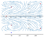
Figure 1: Left: 1591-th entry of the order type database for 8 points [4]. With complex stream plots of its Voronoi polynomial (center): $p_{V}(z)=10+23z+27z^{2}+24z^{3}+17z^{4}+9z^{5}+2z^{6}$, and its $E_{\leq k}$ polynomial (right): $p_{E}(z)=4+13z+22z^{2}+34z^{3}+43z^{4}+52z^{5}$; roots are red points.

For a point set $S$, we show that $\overline{cr}(S)$ appears in the first derivatives of these three polynomials when evaluated at $z=1$ and, in addition, we obtain appealing formulas for $\overline{cr}(S)$ in terms of the roots of the polynomials. Motivated by this, we study the location of such roots, showing several bounds on their modulus. As a particular result, we also prove that the roots of the Voronoi polynomial lie on the unit circle if and only if $S$ is in convex position. Polynomials with zeros on the unit circle have been studied for instance in [13, 14, 22, 23].

Furthermore, the circle polynomial comes into play when considering the random variable $X$ that counts the number of points of $S$ enclosed by the circle defined by three points chosen uniformly at random from $S$. The probability generating function of $X$ is $p_{C}(z)/{{n}\choose{3}}$. In [29] a central limit theorem for random variables with values in $\{0,\ldots,n\}$ was shown, under the condition that the variance is large enough and that no root of the probability generating function is too close to $1\in\mathbb{C}.$ We show that the random variable $X$ does not approximate a normal distribution, and use the result from [29] to derive that $p_{C}(z)$ has a root close to $1\in\mathbb{C}.$

We first state in Section 2 the known relations for Voronoi diagrams, circles enclosing points, and $j$-edges, that we will use. Then, in Section 3, we apply them to obtain properties of the three polynomials. Section 4 is on the roots of the polynomials. Finally, Section 5 discusses open problems, the related polynomial of $j$-edges, and conclusions.

Throughout this work, points $(a,b)$ in the plane are identified with complex numbers $z=a+ib$. To avoid cumbersome notation we omit indicating the point set $S$ where it is clear from context; for example, we write $p_{C}(z)$ instead of $p^{S}_{C}(z)$.

2 Known relations

In this section, necessary results for the current paper are presented. These consist in the relations between the number $c_{k}$ of circles enclosing $k$ points of $S$, the crossing number $\overline{cr}(S)$, the number $E_{\leq k}$ of (at most $k$)-edges of $S$, and the number $v_{k}$ of vertices of the Voronoi diagram of order $k$ of $S$.

A main source is the work by Lee [24], from where several of the following formulas can be obtained.

• For any point set $S$, and $0\leq k\leq n-3$, it holds that, see [9, 15, 16, 24, 26],

  $$c_{k}+c_{n-k-3}=2(k+1)(n-k-2).$$ (2)

• From [18] we get the following two equations.

  $$\sum_{k=0}^{n-3}k\cdot c_{k}={{n}\choose{4}}+\overline{cr}(S)=(1+\alpha){{n}\choose{4}}.$$ (3)

  This was essentially also obtained in [34], though not stated in terms of $\overline{cr}(S)$.

  $$\sum_{k=0}^{n-3}k^{2}\cdot c_{k}={{n}\choose{5}}+{{n}\choose{4}}+(n-3)\overline{cr}(S).$$ (4)

• For $k\leq\frac{n-3}{2}$ it holds that, see Lemma 3.1 in [17],

  $$c_{k}\geq(k+1)(n-k-2)$$ (5)

  and

  $$c_{n-k-3}\leq(k+1)(n-k-2).$$ (6)

• For every set $S$ of $n$ points in general position, the relation between $E_{\leq k}$ and $c_{k}$ is, see e.g. Property 33 in [16],

  $$c_{k}+E_{\leq k}=(k+1)(2n-k-2).$$ (7)

  For a point set $S$ in convex position, we have equality in Equations (5) and (6) which can be derived from Equations (7) and $E_{\leq k}=(k+1)n$ for $S$ in convex position, and therefore,

  $$2c_{k}=c_{k-1}+c_{k+1}+2.$$ (8)

  Then, the number of vertices of $V_{k}(S)$, for $S$ in convex position fulfills, see e.g. Property 34, Equation (4) in [16],

  $$v_{k}=c_{k-1}+c_{k-2}=(2k-1)n-2k^{2}\ .$$ (9)

  Note that, for $S$ in convex position this implies that

  $$v_{k}=v_{n-k}.$$ (10)

3 Properties of the Voronoi, circle and $E_{\leq_{k}}$ polynomials

In the following section, we will show the relations between the Voronoi and the circle polynomials, $p_{V}(z)$ and $p_{C}(z)$. Some additional properties for $p_{V}(z),p_{C}(z)$ and $p_{E}(z)$ will also be presented. Finally, we will give a family of formulas for the crossing number in terms of the coefficients of these three polynomials.

Proposition 1.

For every set $S$ of $n$ points in general position, the circle polynomial $p_{C}(z)=\sum_{k=0}^{n-3}c_{k}z^{k}$ and the Voronoi polynomial $p_{V}(z)=\sum_{k=1}^{n-1}v_{k}z^{k-1}$ satisfy:

$$p_{V}(z)=(1+z)p_{C}(z).$$ (11)

Proof.

This follows from the property $v_{k}=c_{k-1}+c_{k-2},$ for $1\leq k\leq n-1$, where $c_{-1}=0$ and $c_{n-2}=0$. Then,

$$p_{V}(z)=c_{0}+\sum_{k=2}^{n-2}(c_{k-1}+c_{k-2})z^{k-1}+c_{n-3}z^{n-2}=p_{C}(z)+z\cdot p_{C}(z).$$

∎

Proposition 2.

For every set $S$ of $n$ points in general position, the circle polynomial $p_{C}(z)=\sum_{k=0}^{n-3}c_{k}z^{k}$ satisfies:

1. $p_{C}(1)={{n}\choose{3}}.$

2. $p^{\prime}_{C}(1)={{n}\choose{4}}+\overline{cr}(S).$

3. $p^{\prime\prime}_{C}(1)={{n}\choose{5}}+(n-4)\overline{cr}(S).$

4. $p_{C}(-1)=\frac{n-1}{2}$ for $n$ odd.

Proof.

Since there are ${{n}\choose{3}}$ different circles passing through three different points from $S$, the first claim follows. The second one follows from Equation (3). The third equality follows from Equations (3) and (4). Finally, we use Equation (2) to obtain the fourth equality; note that from Equation (2), for $n$ odd it follows that $c_{\frac{n-3}{2}}=\frac{(n-1)^{2}}{4}$.

$$p_{C}(-1)=\sum_{k=0}^{n-3}(-1)^{k}c_{k}=\sum_{k=0}^{\frac{n-3}{2}-1}\left((-1)^{k}2(k+1)(n-2-k)\right)+(-1)^{\frac{n-3}{2}}c_{\frac{n-3}{2}}=\frac{n-1}{2}.$$

∎

When we consider the Voronoi polynomial we get:

Proposition 3.

For every set $S$ of $n$ points in general position, the Voronoi polynomial $p_{V}(z)=\sum_{k=1}^{n-1}v_{k}z^{k-1}$ satisfies:

1. $p_{V}(1)=2{{n}\choose{3}}.$

2. $p^{\prime}_{V}(1)={{n}\choose{3}}+2{{n}\choose{4}}+2\overline{cr}(S).$

3. $p^{\prime\prime}_{V}(1)=2{{n}\choose{4}}+2{{n}\choose{5}}+2(n-3)\overline{cr}(S).$

4. $p_{V}(-1)=0.$

5. $p^{\prime}_{V}(-1)=\frac{n-1}{2}$ for $n$ odd.

Proof.

This follows from Proposition 1 and Proposition 2. From $p_{V}(z)=(1+z)p_{C}(z)$, we get

$$p^{\prime}_{V}(z)=p_{C}(z)+(1+z)\cdot p^{\prime}_{C}(z)$$

and

$$p^{\prime\prime}_{V}(z)=2p^{\prime}_{C}(z)+(1+z)\cdot p^{\prime\prime}_{C}(z).$$

Then just substitute from Proposition 2. The fourth property follows directly from Proposition 1 and was already noted by Lindenbergh [26]. The last property follows from taking derivatives in Proposition 1. ∎

When we consider the $E_{\leq_{k}}$ polynomial we get:

Proposition 4.

For every set $S$ of $n$ points in general position, the $E_{\leq_{k}}$ polynomial $p_{E}(z)=\sum_{k=0}^{n-3}E_{\leq_{k}}z^{k}$ satisfies:

1. $p_{E}(1)=3{{n}\choose{3}}.$

2. $p^{\prime}_{E}(1)=9{{n}\choose{4}}-\overline{cr}(S).$

3. $p^{\prime\prime}_{E}(1)=35{{n}\choose{5}}-(n-4)\overline{cr}(S).$

4. $p_{E}(-1)=\frac{n(n-1)}{2}$ for $n$ odd.

Proof.

The first equality follows from Equation (7) by summing over all $k$, and Proposition 2, part 1. Note that $\sum_{k=0}^{n-3}\left((k+1)(2n-k-2)\right)=4{{n}\choose{3}}$.

$$p_{E}(1)=\sum_{k=0}^{n-3}E_{\leq k}=\sum_{k=0}^{n-3}\left((k+1)(2n-k-2)-c_{k}\right)=4{{n}\choose{3}}-p_{C}(1)=3{{n}\choose{3}}$$

The second and third equalities follow from Equations (3) and (7).

The fourth equality follows from Equation (7) and Proposition 2, part 4. Note that for $n$ odd: $\sum_{k=0}^{n-3}(-1)^{k}\left((k+1)(2n-k-2)\right)=\frac{n^{2}-1}{2}$.

$$p_{E}(-1)=\sum_{k=0}^{n-3}(-1)^{k}E_{\leq k}=\sum_{k=0}^{n-3}(-1)^{k}\left((k+1)(2n-k-2)\right)-p_{C}(-1)=\frac{n(n-1)}{2}$$

∎

From the following result of Aziz and Mohammad, see Lemma 1 in [10], we get an intriguing family of formulas for the rectilinear crossing number in terms of the coefficients of the three studied polynomials, and the roots of a non-zero complex number $a\neq-1$.

Theorem 5 (Aziz and Mohammad, 1980).

If $P(z)$ is a polynomial of degree $n$ and $z_{1},\ldots,z_{n}$ are the zeros of $z^{n}+a$, where $a\neq-1$ is any non-zero complex number, then for any complex number $t$,

$$tP^{\prime}(t)=\frac{n}{1+a}P(t)+\frac{1+a}{na}\sum_{k=1}^{n}P(tz_{k})\frac{z_{k}}{(z_{k}-1)^{2}}.$$

Proposition 6.

The coefficients of the polynomials $p_{V}(z)$, $p_{C}(z)$ and $p_{E}(z)$ satisfy

$$\emph{\bf 1) }\overline{cr}(S)=\sum_{j=0}^{n-3}c_{j}\left(\frac{4}{3(n-3)}\sum_{k=1}^{n-3}\frac{z_{k}^{j+1}}{(z_{k}-1)^{2}}\right),$$ (12)

where the $z_{k}$ are the $(n-3)$-th roots of $-3$.

$$\emph{\bf 2) }\overline{cr}(S)=\sum_{j=1}^{n-1}v_{j}\left(\frac{2}{3(n-1)}\sum_{k=1}^{n-1}\frac{z_{k}^{j}}{(z_{k}-1)^{2}}\right),$$ (13)

where the $z_{k}$ are the $(n-1)$-th roots of $-3$.

$$\emph{\bf 3) }\overline{cr}(S)=\sum_{j=0}^{n-3}E_{\leq j}\left(\frac{-4}{n-3}\sum_{k=1}^{n-3}\frac{z_{k}^{j+1}}{(z_{k}-1)^{2}}\right),$$ (14)

where the $z_{k}$ are now the $(n-3)$-th roots of $-\frac{1}{3}$.

Proof.

Using Theorem 5 for $t=1$ and for the circle polynomial $p_{C}(z)$, we get for any non-zero complex number $a\neq-1$,

$${{n}\choose{4}}+\overline{cr}(S)=\frac{n-3}{1+a}{{n}\choose{3}}+\frac{1+a}{(n-3)a}\sum_{k=1}^{n-3}\sum_{j=0}^{n-3}c_{j}\frac{z_{k}^{j+1}}{(z_{k}-1)^{2}}$$ (15)

Taking $a=3$ we get

$$\overline{cr}(S)=\frac{4}{3(n-3)}\sum_{k=1}^{n-3}\sum_{j=0}^{n-3}c_{j}\frac{z_{k}^{j+1}}{(z_{k}-1)^{2}}=\sum_{j=0}^{n-3}c_{j}\left(\frac{4}{3(n-3)}\sum_{k=1}^{n-3}\frac{z_{k}^{j+1}}{(z_{k}-1)^{2}}\right),$$ (16)

where the $z_{k}$ are the $(n-3)$-th roots of $-3$.

Using Theorem 5 for $t=1$ and for the Voronoi polynomial $p_{V}(z)$, we get for any non-zero complex number $a\neq-1$,

$${{n}\choose{3}}+2{{n}\choose{4}}+2\overline{cr}(S)=\frac{n-1}{1+a}2{{n}\choose{3}}+\frac{1+a}{(n-1)a}\sum_{k=1}^{n-1}\sum_{j=1}^{n-1}v_{j}\frac{z_{k}^{j}}{(z_{k}-1)^{2}}$$ (17)

And again, for $a=3$ we get

$$\overline{cr}(S)=\frac{2}{3(n-1)}\sum_{k=1}^{n-1}\sum_{j=1}^{n-1}v_{j}\frac{z_{k}^{j}}{(z_{k}-1)^{2}}=\sum_{j=1}^{n-1}v_{j}\left(\frac{2}{3(n-1)}\sum_{k=1}^{n-1}\frac{z_{k}^{j}}{(z_{k}-1)^{2}}\right),$$ (18)

where the $z_{k}$ are the $(n-1)$-th roots of $-3$.

Finally, using Theorem 5 for $t=1$ and for the $E_{\leq k}$ polynomial $p_{E}(z)$, we get for any non-zero complex number $a\neq-1$,

$$9{{n}\choose{4}}-\overline{cr}(S)=\frac{3(n-3)}{1+a}{{n}\choose{3}}+\frac{1+a}{(n-3)a}\sum_{k=1}^{n-3}\sum_{j=0}^{n-3}E_{\leq j}\frac{z_{k}^{j+1}}{(z_{k}-1)^{2}}$$ (19)

and taking now $a=\frac{1}{3}$ we get

$$\overline{cr}(S)=-\frac{4}{n-3}\sum_{k=1}^{n-3}\sum_{j=0}^{n-3}E_{\leq j}\frac{z_{k}^{j+1}}{(z_{k}-1)^{2}}=\sum_{j=0}^{n-3}E_{\leq j}\left(\frac{-4}{n-3}\sum_{k=1}^{n-3}\frac{z_{k}^{j+1}}{(z_{k}-1)^{2}}\right),$$ (20)

where the $z_{k}$ are now the $(n-3)$-th roots of $-\frac{1}{3}$. ∎

4 On the roots of Voronoi, circle and $E_{\leq_{k}}$ polynomials

In this section, we present properties of the roots of our polynomials. Note that, by Proposition 1, the Voronoi polynomial $p_{V}(z)$ has the same roots as the circle polynomial $p_{C}(z)$, plus the additional root $z=-1$.

A direct relation between roots of polynomials and the rectilinear crossing number can be derived from the well-known relation

$$\frac{P^{\prime}(z)}{P(z)}=\sum_{i=1}^{n}\frac{1}{z-a_{i}},$$ (21)

where $P(z)$ is a polynomial of degree $n$ with roots $a_{1},\ldots,a_{n}$, and $z$ is any complex number such that $P(z)\neq 0.$

When we consider the circle polynomial $p_{C}(z)$ and $z=1$, using Proposition 2 we get

$$\frac{{{n}\choose{4}}+\overline{cr}(S)}{{{n}\choose{3}}}=\sum_{i=1}^{n-3}\frac{1}{1-a_{i}},$$ (22)

where the $a_{i}$ are the roots of $p_{C}(z)=\sum_{k=0}^{n-3}c_{k}z^{k}.$

Consider the reciprocal polynomial $p^{*}_{C}(z)=\sum_{k=0}^{n-3}c_{k}z^{n-k-3}$ of $p_{C}(z)$. It is well known that the roots of a reciprocal polynomial $p^{*}_{C}(z)$ are $1/a_{i}$ where $a_{i}$ is a root of $p_{C}(z).$

Proposition 7.

$$\sum_{k=0}^{n-3}(n-k-3)c_{k}=3{{n}\choose{4}}-\overline{cr}(S)$$ (23)

Proof.

We use Equation (21). Observe that for a root $a_{i}$ of $p_{C}(z)$ and a root $1/a_{i}$ of $p^{*}_{C}(z)$ we have $\frac{1}{1-a_{i}}+\frac{1}{1-1/a_{i}}=1.$ Then,

$$\frac{p^{\prime}_{C}(1)}{p_{C}(1)}+\frac{p^{*^{\prime}}_{C}(1)}{p^{*}_{C}(1)}=n-3.$$

Equation (23) follows by substituting $p^{\prime}_{C}(1)={{n}\choose{4}}+\overline{cr}(S)$, and $p_{C}(1)=p^{*}_{C}(1)={{n}\choose{3}}.$ ∎

The following equation is obtained in a similar fashion:

Proposition 8.

$$\frac{-2{{n}\choose{4}}+2\overline{cr}(S)}{{{n}\choose{3}}}=\sum_{i=1}^{n-3}\frac{1+a_{i}}{1-a_{i}},$$ (24)

where the $a_{i}$ are the roots of $p_{C}(z)=\sum_{k=0}^{n-3}c_{k}z^{k}.$

Proof.

$$\frac{p^{\prime}_{C}(1)}{p_{C}(1)}-\frac{p^{*^{\prime}}_{C}(1)}{p^{*}_{C}(1)}=\sum_{i=1}^{n-3}\frac{1}{1-a_{i}}-\sum_{i=1}^{n-3}\frac{1}{1-1/a_{i}}=\sum_{i=1}^{n-3}\frac{1+a_{i}}{1-a_{i}}.$$

The left side of this equation simplifies to $\frac{-2{{n}\choose{4}}+2\overline{cr}(S)}{{{n}\choose{3}}}$. ∎

Note that Proposition 8 also works for the roots of the Voronoi polynomial $p_{V}(z)$, since the Voronoi polynomial has the same roots as the circle polynomial, plus the additional root $z=-1$ for which the corresponding term in the sum is zero.

Of particular interest is the polynomial $p_{V}(z)=\sum_{k=1}^{n-1}v_{k}z^{k-1}$ for a set of $n$ points in convex position. By Equation (9), $v_{k}=(2k-1)n-2k^{2}$. By Equation (10), $p_{V}(z)$ is a palindromic polynomial, so it has roots $a_{i}$ and $1/a_{i}$. It follows that for sets $S$ of $n$ points in convex position

$$\sum_{i=1}^{n-2}\frac{1}{1-a_{i}}=\frac{n-2}{2},$$ (25)

where the $a_{i}$ are the roots of $p_{V}(z)=\sum_{k=1}^{n-1}v_{k}z^{k-1}$. We also have that for $S$ in convex position, from Proposition 8,

$$\sum_{i=1}^{n-2}\frac{1+a_{i}}{1-a_{i}}=0.$$ (26)

For our next result we use the following theorem due to Malik [28], also see the book by Rahman and Schmeisser [33], Corollary 14.4.2.

Theorem 9 (Rahman and Schmeisser, 2002).

Let $f$ be a polynomial of degree $n$ having all its zeros in the closed disk $|z|\leq k$, where $k\leq 1$. Then

$$\max_{|z|=1}|f^{\prime}(z)|\geq\frac{n}{1+k}\max_{|z|=1}|f(z)|.$$

Theorem 10.

Let $S$ be a set of $n$ points in general position in the plane. Then $S$ is in convex position if and only if all the roots of the Voronoi polynomial of $S$, $p_{V}(z)=\sum_{k=1}^{n-1}v_{k}z^{k-1}$, lie on the unit circle.

Proof.

In view of Proposition 1, we can consider the circle polynomial $p_{C}(z)$ instead of the Voronoi polynomial.

If all the roots of $p_{C}(z)$ lie on the unit circle, in particular they are contained in the closed unit disk. Thus, we can apply Theorem 9 to the circle polynomial. Since all its coefficients are positive, $\max_{|z|=1}|f^{\prime}(z)|=f^{\prime}(1)$ and $\max_{|z|=1}|f(z)|=f(1)$. We get

$${{n}\choose{4}}+\overline{cr}(S)\geq\frac{n-3}{1+k}{{n}\choose{3}}.$$

Observing that $(n-3){{n}\choose{3}}=4{{n}\choose{4}}$ and $k\leq 1$, this simplifies to

$$\overline{cr}(S)\geq{{n}\choose{4}}\frac{3-k}{1+k}\geq{{n}\choose{4}}.$$

Then, since the inequality $\overline{cr}(S)\leq{{n}\choose{4}}$ always holds, we have $\overline{cr}(S)={{n}\choose{4}}$, which implies that (is actually equivalent to) $S$ being in convex position.

It remains to show that for a point set $S$ in convex position all its roots lie on the unit circle. For $S$ in convex position we have equality in Equations (5) and (6), which implies that $p_{C}(z)$ is a palindromic polynomial. By Equation (8), for $S$ in convex position the coefficients of $p_{C}(z)$ satisfy $2c_{k}=c_{k-1}+c_{k+1}+2$. For a palindromic polynomial (with say coefficients $c_{k}$) that satisfies $2c_{k}\geq c_{k-1}+c_{k+1}$ it is known that all its roots lie on the unit circle, see e.g. [13], Theorem 2.5. ∎

In order to find a lower bound on the largest modulus of the roots of $p_{C}(z)$ with $S$ not in convex position, we use the following two theorems. The first one is due to Laguerre [21], Theorem 1, see also Nagy [30], and Rahman and Schmeisser [33], Theorem 3.2.1b.

Theorem 11 (Rahman and Schmeisser, 2002).

Let $f$ be a polynomial of degree $n\geq 2$. If $\zeta$, belonging to the complex plane, is neither a zero nor a critical point of $f$, then every circle $C$ that passes through $\zeta$ and $\zeta-n\frac{f(\zeta)}{f^{\prime}(\zeta)}$ separates at least two zeros of $f$ unless the zeros all lie on $C$.

The second theorem is due to Obrechkoff [31], also see Bergweiler and Eremenko [11] and Marden [27], Chapter IX,41, Exercise 5.

Theorem 12 (Obrechkoff, 1923).

For every polynomial $P$ of degree $n$ with non-negative coefficients and every $\theta\in\left(0,\frac{\pi}{2}\right)$, the number of roots in the sector $\{z\in\mathbb{C}\backslash\{0\}\ |\ \ |arg(z)|\leq\theta\}$ is at most $\frac{2\theta n}{\pi}$.

Theorem 13.

For every set $S$ of $n>3$ points in general position with rectilinear crossing number $\overline{cr}(S)=\alpha\cdot{{n}\choose{4}}$, the Voronoi polynomial $p_{V}(z)=\sum_{k=1}^{n-1}v_{k}z^{k-1}$ has a root of modulus at least $1+\frac{(1-\alpha)\pi^{2}}{16(n-3)^{2}}+O\left(\frac{1}{n^{4}}\right)$.

Proof.

First observe that if $S$ is in convex position, then $\alpha=1$ and the statement of the theorem holds by Theorem 10. Assume then that $S$ is not in convex position. Therefore, not all points of $S$ lie on a common circle. We apply Theorem 11 to the circle polynomial $p_{C}(z)=\sum_{k=0}^{n-3}c_{k}z^{k}$ and $\zeta=1.$ Thus, by Proposition 2, every circle $C$ passing through point $(1,0)$ and through point $\left(1-\frac{(n-3){{n}\choose{3}}}{{{n}\choose{4}}+\overline{cr}(S)},0\right)=\left(1-\frac{4}{1+\alpha},0\right)$ separates at least two zeros of $p_{C}(z)$. The center of the smallest such circle $C^{s}$ is $(\frac{\alpha-1}{\alpha+1},0)$, and the radius of $C^{s}$ is $\frac{2}{1+\alpha}.$ Let $D^{s}$ denote the disk with boundary the circle $C^{s}$.
The unit disk is contained in $D^{s}$, touching it in the point $(1,0)$. This already shows that there exists a zero of $p_{C}(z)$ that lies outside of the unit disk.

From Obrechkoff’s inequality, Theorem 12, we obtain that the sector $T=\{z\in\mathbb{C}\backslash\{0\}\ |\ \ |arg(z)|<\frac{\pi}{2(n-3)}\}$ is empty of roots of $p_{C}(z)$.

By Theorems 11 and 12, the region $\mathbb{C}\backslash(D^{s}\cup T)$ contains a root of $p_{C}(z)$. Then, the modulus of the largest root of $p_{C}(z)$ is at least the distance $d$ from the origin to the intersection point in the first quadrant of $C^{S}$ with the line $y=\tan{\left(\frac{\pi}{2(n-3)}\right)}x$ for $n>4$; see Figure 2.

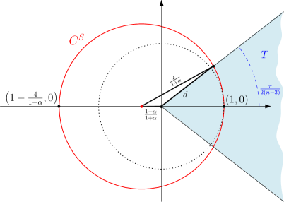
Figure 2: The sector $T=\{z\in\mathbb{C}\backslash\{0\}\ |\ \ |arg(z)|<\frac{\pi}{2(n-3)}\}$ is empty of roots of $p_{C}(z)$. The region $\mathbb{C}\backslash(D^{s}\cup T)$ contains a root of $p_{C}(z)$, with modulus at least $d$. The unit circle is drawn dotted.

This distance $d$ satisfies, see Figure 2,

$$\left(\frac{2}{1+\alpha}\right)^{2}=\left(\frac{\alpha-1}{\alpha+1}\right)^{2}+d^{2}-2d\frac{1-\alpha}{1+\alpha}\cos{\left(\pi-\frac{\pi}{2(n-3)}\right)}.$$

Since $\cos{\left(\pi-\frac{\pi}{2(n-3)}\right)}=-\cos{\left(\frac{\pi}{2(n-3)}\right)}$, we get

$$d^{2}+2d\frac{1-\alpha}{1+\alpha}\cos{\left(\frac{\pi}{2(n-3)}\right)}+\frac{\alpha-3}{1+\alpha}=0,\ \mbox{and then}$$

$$d=\frac{(-1+\alpha)\cos{\left(\frac{\pi}{2(n-3)}\right)}+\sqrt{\cos^{2}{\left(\frac{\pi}{2(n-3)}\right)}(-1+\alpha)^{2}-\alpha^{2}+2\alpha+3}}{1+\alpha}.$$

For $\alpha$ fixed, the Taylor polynomial of

$$f(x)=\frac{(-1+\alpha)\cos{x}+\sqrt{\cos^{2}{x}(-1+\alpha)^{2}-\alpha^{2}+2\alpha+3}}{1+\alpha}$$

of degree four at the point $0$ is

$$1+\frac{1-\alpha}{4}x^{2}+\frac{-3\alpha^{3}+5\alpha^{2}-17\alpha+5}{192}x^{4}.$$

Then

$$d=f\left(\frac{\pi}{2(n-3)}\right)=1+\frac{(1-\alpha)\pi^{2}}{16(n-3)^{2}}+O\left(\frac{1}{n^{4}}\right).$$

∎

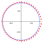
Figure 3: Left: Best known example for minimizing $\overline{cr}(S)$ for $|S|=100$  [5]. Roots of its Voronoi (center), and $E_{\leq k}$ (right) polynomials, with circles illustrating, respectively, the bounds of Theorems 13 and 18.

We further show that the Voronoi polynomial $p_{V}(z)$ has a root close to point $1$ in the complex plane. For this, we use Theorem 1.2 from Michelen and Sahasrabudhe [29].

Theorem 14 (Michelen and Sahasrabudhe, 2019).

Let $X\in\{0,\ldots,n\}$ be a random variable with mean $\mu$, standard deviation $\sigma$ and probability generating function $f_{X}$ and set $X^{*}=(X-\mu)\sigma^{-1}.$ If $\delta\in(0,1)$ is such that $|1-\zeta|\geq\delta$ for all roots $\zeta$ of $f_{X}$ then

$$\sup_{t\in\mathbb{R}}|\mathbb{P}(X^{*}\leq t)-\mathbb{P}(Z\leq t)|=O\left(\frac{\log{n}}{\sigma\delta}\right),$$ (27)

where $Z\sim N(0,1).$

Theorem 15.

Let $\alpha$ be a constant from $(0,1]$ and let $S$ be a set of $n$ points in general position in the plane with $\frac{\overline{cr}(S)}{{{n}\choose{4}}}=\alpha$. Then, the Voronoi polynomial of $S$, $p_{V}(z)=\sum_{k=1}^{n-1}v_{k}z^{k-1}$, has a root $\zeta$ such that $|1-\zeta|\in o\left(\frac{log{(n)}}{n}\right).$

Proof.

Let $X$ be the random variable that counts the number of points of $S$ enclosed by the circle defined by three points chosen uniformly at random from $S$. The probability generating function $f_{X}$ of $X$ is $p_{C}(z)/{{n}\choose{3}}$. The roots of $f_{X}$ are also roots of $p_{V}(z)$, by Proposition 1. From Equations (3) and (4), see [18], the mean of $X$ is $\mu=\sum_{k=0}^{n-3}k\cdot\frac{c_{k}}{{{n}\choose{3}}}=\frac{p^{\prime}_{C}(1)}{p_{C}(1)}=\frac{(1+\alpha)\cdot(n-3)}{4}$ and the standard deviation of $X$ is $\sigma=\sqrt{\frac{p^{\prime\prime}_{C}(1)+p^{\prime}_{C}(1)}{p_{C}(1)}-\left(\frac{p^{\prime}_{C}(1)}{p_{C}(1)}\right)^{2}}=(n-3)\cdot\sqrt{\frac{\alpha}{8}-\frac{\alpha^{2}}{16}-\frac{1}{80}+\frac{1}{5(n-3)}}.$ For $\delta\in o\left(\frac{log{(n)}}{n}\right)$, we have $\sigma\delta(\log n)^{-1}\rightarrow\infty$. In order to apply Theorem 14, it remains to show that $X$ does not approach a normal distribution when $n$ tends towards infinity. For $t=0$ in Equation (27), we get from Proposition 2,

$$P(X^{*}\leq 0)=\mathbb{P}(X\leq\mu)=\mathbb{P}\left(X\leq\frac{(1+\alpha)(n-3)}{4}\right).$$

By Equation (5), $\mathbb{P}(X=k)\geq\frac{(k+1)(n-k-2)}{{{n}\choose{3}}}$ holds for $k<\frac{n-3}{2}.$ Then

$$\mathbb{P}(X\leq\mu)\geq\sum_{k=0}^{(1+\alpha)(n-3)/4}\frac{(k+1)(n-k-2)}{{{n}\choose{3}}}\geq\frac{(5-\alpha)(1+\alpha)^{2}}{32}-O\left(\frac{1}{n}\right).$$

For $\alpha<1$,

$$\lim_{n\rightarrow\infty}|\mathbb{P}(X^{*}\leq 0)-\mathbb{P}(Z\leq 0)|=\left|\frac{(5-\alpha)(1+\alpha)^{2}}{32}-O\left(\frac{1}{n}\right)-\frac{1}{2}\right|>0,$$

but $\lim_{n\rightarrow\infty}\frac{\log{n}}{\sigma\delta}=0.$ Then, Equation (27) does not hold for $n$ large enough. It follows that there exists a root $\zeta$ of $f_{X}$ with $|1-\zeta|<\delta$.

For $\alpha=1$, we know $f_{X}$ precisely. $S$ is a set of $n$ points in convex position and $c_{k}=(k-1)(n-k-2)$ for every $0\leq k\leq n-3$. By Equation (8), $f_{X}$ is a concave function. Then $X$ does not approach a normal distribution also for $\alpha=1.$ It follows that there exists a root $\zeta$ of $f_{X}$ with $|1-\zeta|<\delta$. ∎

Note that on the other hand, Obrechkoff’s Theorem 12 implies that no root of the Voronoi polynomial can be too close to point 1 in the complex plane. Indeed, the largest disk centered at 1 and contained in the sector $T$ bounded by the two lines $y=\pm\tan\left(\frac{\pi}{2(n-3)}\right)$ in the right half-plane (see Figure 2) given by Obrechkoff’s Theorem, has radius $r=\sin\left(\frac{\pi}{2(n-3)}\right)$. Then, the distance of the closest root to point 1 is at least $r\geq\sin\left(\frac{\pi}{2(n-3)}\right)\geq\frac{1}{n-3}$.

In the following, we study the location of the roots of the $E_{\leq k}$ polynomial $p_{E}(z)=\sum_{k=0}^{n-3}E_{\leq k}z^{k}$ of a point set $S$. Note that its coefficients $E_{\leq k}$ form an increasing sequence of positive numbers. The well-known Eneström-Kakeya theorem [20] tells us that all the roots of $p_{E}(z)$ are contained in the unit disk, and more precisely, that they are contained in an annulus: The absolute values of the roots of $p_{E}(z)$ lie between the greatest and the least of the $n-3$ quotients

$$\frac{E_{\leq n-4}}{E_{\leq n-3}},\frac{E_{\leq n-5}}{E_{\leq n-4}},\ldots,\frac{E_{\leq 1}}{E_{\leq 2}},\frac{E_{\leq 0}}{E_{\leq 1}}.$$

We give a lower bound on the largest modulus of the roots of the $E_{\leq k}$ polynomial.

Theorem 16.

Let $S$ be a set of $n>3$ points in general position in the plane, with rectilinear crossing number $\overline{cr}(S)=\alpha\cdot{{n}\choose{4}}$. Then, the $E_{\leq k}$ polynomial of $S$, $p_{E}(z)=\sum_{k=0}^{n-3}E_{\leq k}z^{k}$, has a root of modulus at least $\frac{3+\alpha}{9-\alpha}.$

Proof.

From Proposition 4 we get

$$\frac{p_{E}^{\prime}(1)}{p_{E}(1)}=\frac{9{{n}\choose{4}}-\overline{cr}(S)}{3{{n}\choose{3}}}=\frac{(9-\alpha)\cdot(n-3)}{12}=\sum_{j=1}^{n-3}\frac{1}{1-a_{j}},$$ (28)

where the $a_{j}$, for $j=1,\ldots,n-3,$ are the roots of $p_{E}(z)$.

The conjugate of a complex number $w=a+ib$ is denoted as $\overline{w}=a-ib$. The following identity which holds for any complex number $w\neq 1$ is easily verified:

$$\frac{1}{1-w}+\frac{1}{1-\overline{w}}=1+\frac{1-|w|^{2}}{|1-w|^{2}}.$$ (29)

Since all the coefficients of $p_{E}(z)$ are real numbers, the non-real roots of $p_{E}(z)$ come in pairs, $a_{j}$ together with its conjugate $\overline{a_{j}}.$ We apply Equation (29) to each such pair $w=a_{j}$ and $\overline{w}=\overline{a_{j}}.$ For each real root $a_{j}$ of $p_{E}(z)$, Equation (29) gives

$$\frac{1}{1-a_{j}}=\frac{1}{2}\left(1+\frac{1-|a_{j}|^{2}}{|1-a_{j}|^{2}}\right).$$

Then,

$$\sum_{j=1}^{n-3}\frac{1}{1-a_{j}}=\sum_{j=1}^{n-3}\frac{1}{2}\left(1+\frac{1-|a_{j}|^{2}}{|1-a_{j}|^{2}}\right).$$

We substitute into Equation (28) and obtain

$$\frac{(n-3)\cdot(3-\alpha)}{6}=\sum_{j=1}^{n-3}\frac{1-|a_{j}|^{2}}{|1-a_{j}|^{2}}.$$ (30)

The next inequality, which holds for every complex number $w\neq 1$ with modulus $|w|<1$ is easily verified.

$$\frac{1-|w|^{2}}{|1-w|^{2}}\geq\frac{1-|w|}{1+|w|}$$ (31)

Since the coefficients of $p_{E}(z)$ form an increasing sequence of positive numbers, the roots $a_{j}$ of $p_{E}(z)$ all satisfy $|a_{j}|<1.$ We use Inequation (31) in Equation (30). Then,

$$\frac{(n-3)\cdot(3-\alpha)}{6}\geq(n-3)\cdot\min_{\begin{subarray}{c}|a_{j}|\\ j=1,\ldots,n-3\end{subarray}}\frac{1-|a_{j}|}{1+|a_{j}|}.$$

Note that the function $f(x)=\frac{1-x}{1+x}$ is decreasing for $x\in(0,1).$ Then, the minimum of $\frac{1-|a_{j}|}{1+|a_{j}|}$ is attained when $|a_{j}|$ is maximum. It follows that $|a_{max}|=\max_{\begin{subarray}{c}|a_{j}|\\ j=1,\ldots,n-3\end{subarray}}\geq\frac{3+\alpha}{9-\alpha}$, by solving for $|a_{max}|$ in

$$\frac{(n-3)\cdot(3-\alpha)}{6}\geq(n-3)\cdot\frac{1-|a_{max}|}{1+|a_{max}|}.$$ (32)

This completes the proof. ∎

Next, we show a better lower bound on the largest modulus of $p_{E}(z)$ when $n$ is large enough. For this, we use the following theorem of Titchmarsh ([36], page 171), also see Gardner and Shields [19], Theorem A.

Theorem 17 (Gardner and Shields, 2013).

Let $F(z)$ be analytic in $|z|\leq R.$ Let $|F(z)|\leq M$ in the disk $|z|\leq R$ and suppose $F(0)\neq 0$. Then, for $0<\delta<1$, the number of zeros of $F(z)$ in the disk $|z|\leq\delta R$ is less than

$$\frac{1}{\log{\frac{1}{\delta}}}\log{\frac{M}{|F(0)|}}.$$

Theorem 18.

Let $S$ be a set of $n$ points with $h$ of them on the boundary of the convex hull of $S$, in general position in the plane. Then $p_{E}(z)=\sum_{k=0}^{n-3}E_{\leq k}z^{k}$ has a root of modulus at least

$$\left(\frac{3{{n}\choose{3}}}{h}\right)^{-\frac{1}{n-3}}.$$

Proof.

By the maximum modulus principle and Proposition 4, $|p_{E}(z)|\leq 3{{n}\choose{3}}$ in the disk $|z|\leq 1$, and $p_{E}(0)=E_{\leq 0}=h\neq 0.$ We apply Theorem 17 with a large $\delta$ from the interval $(0,1)$ such that

$$\frac{1}{\log{\frac{1}{\delta}}}\log{\frac{3{{n}\choose{3}}}{h}}<n-3.$$

Then, $p_{E}(z)$ has at least one root of modulus greater than $\delta.$ Solving for $\delta$, we obtain that $\delta<\left(\frac{3{{n}\choose{3}}}{h}\right)^{-\frac{1}{n-3}}$. ∎

For an illustration of Theorem 18, see Figure 3 (right) on page 3.

5 Discussion

We have introduced three polynomials $p_{V}(z)$, $p_{C}(z)$, $p_{E}(z)$ for sets $S$ of $n$ points in general position in the plane, showing their connection to $\overline{cr}(S)$ and several bounds on the location of their roots. The obvious open problem is using bounds on such roots to improve upon the current best bound on the rectilinear crossing number problem. Besides, we think that the presented polynomials are interesting objects of study on their own, also given the many applications of Voronoi diagrams.

For some of the formulas presented for one of the polynomials, such as for example Equations (22) and (30), there are analogous statements for the other considered polynomials. These can be derived easily and are omitted.

Further, several other polynomials on point sets can be considered. The reader interested in crossing numbers probably has in mind the $j$-edge polynomial $p_{e}(z)=\sum_{j=0}^{n-2}e_{j}z^{j}$ of a point set $S$. The known formula for the rectilinear crossing number $\overline{cr}(S)$ in terms of the numbers of $j$-edges $e_{j}$ of $S$, see [25], Lemma 5, translates into

$$2\overline{cr}(S)-6{{n}\choose{4}}=p^{\prime\prime}_{e}(1)-(n-3)p^{\prime}_{e}(1).$$

As is the case for the Voronoi polynomial and the circle polynomial, for sets $S$ of $n$ points in convex postion, the $j$-edge polynomial $p_{e}(z)$ has all its roots on the unit circle. This is readily seen since $p_{e}(z)$ is then $n$ times the all ones polynomial, $p_{e}(z)=n\sum_{j=0}^{n-2}z^{j}$, as $e_{j}=n$ for all $j$, if $S$ is in convex position. Its roots are the $(n-1$)th roots of unity, except $z=1.$

We finally propose to study the presented polynomials for random point sets. The expected rectilinear crossing number is known for sets of $n$ points chosen uniformly at random from a convex set $K$, for several shapes of $K$, see e.g. [35], Section 1.4.5. pp. 63-64, and the survey [3].

Acknowledgments.

M. C., A. d.-P., C. H., and D. O. were supported by project PID2019-104129GB-I00/MCIN/AEI/10.13039/501100011033. C.H. was supported by project Gen. Cat. DGR 2021-SGR-00266. D. F.-P. was supported by grants PAPIIT IN120520 and PAPIIT IN115923 (UNAM, México).

References

- [1] B.M. Ábrego, M. Cetina, S. Fernández-Merchant, J. Leaños, G. Salazar, On -edges, crossings, and halving lines of geometric drawings of . Discrete and Computational Geometry 48, 192–215, 2012.
- [2] B.M. Ábrego, S. Fernández-Merchant, A lower bound on the rectilinear crossing number. Graphs and Combinatorics 21, 293–300, 2005.
- [3] B. M. Ábrego, S. Fernández-Merchant, G. Salazar, The rectilinear crossing number of : Closing in (or are we?), Thirty Essays on Geometric Graph Theory, pp. 5–18, Springer, 2012.
- [4] O. Aichholzer, http://www.ist.tugraz.at/aichholzer/research/rp/triangulations/ordertypes/, accessed April 2023.
- [5] O. Aichholzer, http://www.ist.tugraz.at/staff/aichholzer/research/rp/triangulations/crossing/, accessed April 2023.
- [6] O. Aichholzer, J. García, D. Orden, P. Ramos, New lower bounds for the number of - edges and the rectilinear crossing number of , Discrete and Computational Geometry 38, 1–14, 2007.
- [7] F. Aurenhammer. Voronoi diagrams - a survey of a fundamental geometric data structure. ACM Computing Surveys 23(3), 345–405, 1991.
- [8] N. Alon, E. Győri, The number of small semi-spaces of a finite set of points in the plane, Journal of Combinatorial Theory, Series A. 41, 154–157, 1986.
- [9] F. Ardila, The number of halving circles, American Mathematical Monthly 111 (2004), 586–591.
- [10] A. Aziz, Q.G. Mohammad, Simple proof of a theorem of Erdős and Lax. Proceedings of the American Mathematical Society 80, 119–122, 1980.
- [11] W. Bergweiler, A. Eremenko, Distribution of zeros of polynomials with positive coefficients, Annales Academiae Scientiarum Fennicae Mathematica 40, 375–383, 2015.
- [12] J. Balogh, G. Salazar, k-sets, convex quadrilaterals, and the rectilinear crossing number of , Discrete and Computational Geometry 35, 671–690, 2006.
- [13] F. Chapoton, G.-N. Han. On the roots of the Poupard and Kreweras polynomials. Moscow Journal of Combinatorics and Number Theory, 9(2), 163–172, 2020.
- [14] W. Chen, On the Polynomials with All Their Zeros on the Unit Circle, Journal of Mathematical Analysis and Applications, 190(3), 714–724, 1995
- [15] K.L. Clarkson, P.W. Shor, Applications of random sampling in Computational Geometry, II, Discrete Computational Geometry 4, 387–421, 1989.
- [16] M. Claverol, A. de las Heras Parrilla, C. Huemer, A. Martínez-Moraian, The edge labeling of higher order Voronoi diagrams. arxiv: https://arxiv.org/abs/2109.13002, 2021.
- [17] M. Claverol, C. Huemer, A. Martínez-Moraian, On circles enclosing many points, Discrete Mathematics 344(10), 112541, 2021.
- [18] R. Fabila-Monroy, C. Huemer, E. Tramuns, The expected number of points in circles, 28th European Workshop on Computational Geometry (EuroCG 2012), 69–72, 2012. https://www.eurocg.org/2012/booklet.pdf
- [19] R. Gardner, B. Shields, The number of zeros of a polynomial in a disk, Journal of Classical Analysis 3, 167–176, 2013.
- [20] S. Kakeya, On the limits of the roots of an algebraic equation with positive coefficients, Tôhoku Mathematical Journal 2, 140–142, 1912.
- [21] M. Laguerre, Sur la résolution des équations numériques, Nouvelles annales de mathématiques (2) 17, 20–25, 1878.
- [22] P. Lakatos, L. Losonczi, Self-inversive polynomials whose zeros are on the unit circle. Publicationes Mathematicae Debrecen, 65(3-4), 409–420, 2004.
- [23] M. N. Lalín, C. J. Smyth, Unimodularity of zeros of self-inversive polynomials, Acta Mathematica Hungarica, 138, 85–101, 2013.
- [24] D.T. Lee, On -nearest neighbor Voronoi diagrams in the plane, IEEE Transactions on Computers. 31, 478–487, 1982.
- [25] L. Lovász, K. Vesztergombi, U. Wagner, E. Welzl, Convex quadrilaterals and -sets. Towards a theory of geometric graphs, Contemporary Mathematics 342, 139–148. American Mathematical Society, Providence, RI, 2004.
- [26] R.C. Lindenbergh, A Voronoi poset, Journal for Geometry and Graphics. 7, 41–52, 2003.
- [27] M. Marden, The geometry of polynomials, Volume 3 of American Mathematical Society Mathematical Surveys, 1966.
- [28] M.A. Malik, On the derivative of a polynomial, Journal of the London Mathematical Society s2-1(1), 57–60, 1969.
- [29] M. Michelen, J. Sahasrabudhe, Central limit theorems and the geometry of polynomials. arxiv: https://arxiv.org/abs/1908.09020 , 2019.
- [30] Sz. Nagy, Julius von, Über einen Satz von Laguerre, Journal für die reine und angewandte Mathematik, 169, 186–192, 1933.
- [31] N. Obrechkoff, Sur un problème de Laguerre, Comptes Rendus 177, 102–104, 1923.
- [32] A. Okabe, B. Boots, K. Sugihara, S.N. Chiu. Spatial Tessellations: Concepts and Applications of Voronoi diagrams, second edition, Wiley, 2000.
- [33] Q.I. Rahman, G. Schmeisser, Analytic theory of polynomials. London Mathematical Society Monographs New Series 26, Clarendon Press, Oxford, 2002.
- [34] J. Urrutia, A containment result on points and circles. Preprint, February 2004. https://www.matem.unam.mx/~urrutia/online_papers/PointCirc2.pdf
- [35] L. Santaló, Integral geometry and geometric probability, 2nd edition, Cambridge University Press, 2004.
- [36] E.C. Titchmarsh, The theory of functions, 2nd edition, Oxford University Press, London, 1939.