Algebraic and geometric characterization related to the quantization problem of channel $C_{2,8}$

Abstract: In this paper we consider the steps to be followed in the analysis and interpretation of the quantization problem related to the $C_{2,8$channel,wheretheFuchsiandifferentialequations,thegeneratorsoftheFuchsiangroupsandthetessellationsassociatedwiththecases$g=2$and$g=3$,relatedtothehyperboliccase,aredetermined.Inordertoobtaintheseresults,itisnecessarytodeterminethegenus$g$ofeachsurfacewhichthischannelmaybeembedded.Afterthat,theprocedureistodeterminethealgebraicstructure(Fuchsiangroupgenerators)associatedwiththefundamentalregionofeachsurface.Todothis,thereexistsanassociatedlinearsecondorderFuchsiandifferentialequationwhoselinearlyindependentsolutionsprovidethegeneratorsofthisFuchsiangroup.Inaddition,thetessellationsassociatedwitheachoftheanalyzedcasesareidentified.Thesestructuresareidentifiedinfoursituations,dividedintotwocases$(g=2$and$g=3)$,obtainingthereforebothalgebraicandgeometriccharacterizationsassociatedwiththequantizationofthe$C_{2,8}$channel.}\par\\ \par\noindent{\bf Keywords:}{\it FuchsianDifferentialEquations;HyperbolicGeometry;CommunicationSystem;ChannelQuantizationProblem.}\par$

1 Introduction

A communication system can be considered as a set of mechanisms that enables the transmission of information from a transmitter to a given receiver through a communication channel, that can present a series of disturbances, such as a distorsion, for example, which is a noise that can difficult the understanding of the the data sent.

The goals in designing a digital communication system are, basically, to construct systems which are more reliable and less complex than the previously known ones. To achieve these goals, the concept of a metric space $(E_{i},d_{i})$ associated with each block in the traditional model of a communication system is employed, as shown in Fig. 1, according to [canal].

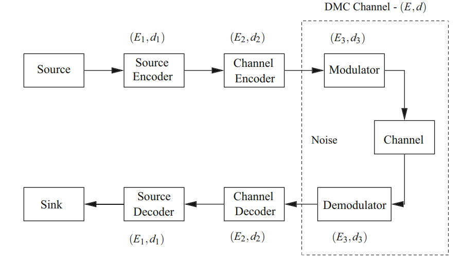
Figura 1: Communication system model, from [canal].

In order to the system to be more reliable, the error probability has to be the lowest possible, whereas to be less complex, it is required that the signal set has to be geometrically uniform, [forney]. These goals may be achieved if the new approach makes use of an important topological invariant known as the genus $g$ of an oriented compact surface where the set of points (signal set) lies. To obtain the genus of the surface one has to find the possible embeddings of the associated discrete memoryless channel on such an oriented compact surface. It is well-known that the geometric uniformity of a signal set $S$ is a property associated with its group of isometry. If the genus is greater than or equal to two, the extension of this concept to the hyperbolic plane implies knowing the hyperbolic isometries as well as its geometric properties.

Massey showed in [massey] that, under the error probability criterion, the performance of a binary digital communication system using soft-decision in the demodulator, for instance, an $8$-level quantizer, leading to a binary input, $8$-ary output symmetric channel, denoted by $C_{2,8}$, achieves a gain of up to 2 dB when compared to the performance of a binary digital communication system using hard-decision (a $2$-level quantizer, leading to a binary symmetric channel (BSC), denoted by $C_{2,2}$).

By performing a 3-bit quantization (8-level quantizer), Massey showed that a surface shift occurs, with the genus greater than the typical $C_{2,2}$ channel, whose associated genus is zero. Based on this fact, there exists a performance gain in the communication process, that is, mathematically, what provides this gain is the invariant genus.

This gain of up 2 dB presented in [massey] comes from the analysis of the performance of the $C_{2,2}$ channel compared to the quantized channel. However, as this process is associated with the change the genus of the associated surface, one of the ways to obtain and use these results comes from through the uniformity regions associated with the process, which, among other ways, can be obtained from a particular class of ordinary differential equations, the Fuchsian differential equations.

Fuchsian differential equations represent an important class of ordinary differential equations, whose main characteristic lies in the fact that every singular point in the extended complex plane is regular. These differential equations are widely used in Mathematical Physics problems and the most studied cases are those involving equations with three regular singular points, such as the hypergeometric, Legendre, and Tchebychev equations, while the Heun equation contains four regular singular points.

In [canal], it is presented a relationship between the singularities of Fuchsian differential equations and hyperbolic geometry, where the singularities of the hypergeometric equation, with three regular singular points, and a Heun equation, with four regular singular points, are seen as fundamental polygons of hyperbolic geometry, in addition to analyze the connection with the channel quantization process, important in the situations involving the transmission of information in a communication systems.

By taking a Fuchsian equation with six singular points, it is shown that there is no equality between the genus of the curve and the genus of the fundamental region; consequently, it is not possible to determine the region for the uniformization of the curve in this case. Thus, there exists a restriction associated with the number of singularities so that genus equality can be achieved. For the other cases, it is necessary to utilize some procedures such as the situations analyzed in this paper.

In [Whittaker, Whittaker2, Mursi], relevant connections are made among Fuchsian differential equations, Riemann surfaces and Fuchsian groups associated with them, in order to analyze the uniformization of the algebraic curves of the form $y^{2}=z^{2g+1}\pm 1$.

The model proposed in [Whittaker] represents a Fuchsian differential equation whose coefficient associated with the highest order derivative is $z^{5}+1$. Through this equation, it is identified that the singularities represent vertices of a polygon; in this particular case, a pentagon. Taking the midpoint of each of the sides of this polygon, it is fixed one of them and, from that side, find the diagonally opposite edge, generating thus an eight-sided polygon, whose maximum associated genus surface is the bitorus.

Similar to the case proposed by [Whittaker], in [Mursi] it is considered a Fuchsian differential equation whose coefficient associated with the highest order derivative $z^{7}+1$. It was identified the singularities associated with the equation and represented as vertices of a polygon of seven sides. Taking the midpoint of each side of this polygon and fixing one of them, the diagonally opposite edge is found, generating a twelve-sided polygon. As a consequence, the associated Riemann surface is the tritorus.

It can be shown that the $C_{2,8}$ channel may be embedded on oriented compact surfaces with genus ranging from zero to three, that is, $0\leq g\leq 3$. For genus $g=0,1$, the geometry is the Euclidean one. The geometric and algebraic structures related to the Euclidean case have been presented in [canal]. In case of genus $g=2,3$, the scenario is the hyperbolic geometry. We consider the cases where $g=2$ and $g=3$ (hyperbolic case) and we divided in four situations:

• for genus $g=2$: the hyperelliptic curve (Whittaker surface) is given by $y^{2}=(z^{5}-1)$, leading to the $n=5$ symmetric points $s_{1},s_{2},\ldots,s_{5}$;

• for genus $g=2$: the hyperelliptic curve is given by $y^{2}=(z^{6}-1)$, leading to the $n=6$ symmetric points $s_{1},s_{2},\ldots,s_{6}$;

• for genus $g=3$: the hyperelliptic curve (Mursi surface) is given by $y^{2}=(z^{7}-1)$, leading to the $n=7$ symmetric points $s_{1},s_{2},\ldots,s_{7}$;

• for genus $g=3$: the hyperelliptic curve is given by $y^{2}=(z^{8}-1)$, leading to the $n=8$ symmetric points $s_{1},s_{2},\ldots,s_{8}$.

It is worth noting that for the two cases analyzed for genus 2 (the curves $y^{2}=(z^{5}-1)$ and $y^{2}=(z^{6}-1)$) and the two cases investigated for genus 3 (the curves $y^{2}=(z^{7}-1)$ and $y^{2}=(z^{8}-1)$), the groups are not isomorphic. However, through the calculations performed, different uniformed regions may be derived, obtaining the associated topology, which can be applied in different situations involving the search for codes with better performance than those already known; for example, in the case involving generalized concatenated codes, through the partitioning of the constellation of signals associated with these codes, in order to obtain a decomposition chain and, consequently, the code alphabet.

This partitioning process makes it possible to obtain normal subgroups from the Fuchsian groups obtained in the process of uniformization of the algebraic curves, allowing engineers and cryptographers, among others, to utilize this mathematical tool in the construction process of new, more reliable and less complex communication systems.

The aim of this paper is to present the algebra (Fuchsian groups generators) and geometry (polygon side pairings and associated tesselations) related to the cases $g=2$ and $g=3$, in order to analyze the channel $C_{2,8}$ quantization problem, which can be embedded in surfaces of genus $0\leq g\leq 3$, through a second order Fuchsian differential equation.

This paper is organized as follows. In Section 2 are presented the main concepts related to graphs and surfaces, hyperbolic geometry, Fuchsian differential equations and the uniformization of the algebraic curves, with the procedure proposed by Whittaker and Mursi to identify the generators of the Fuchsian group. In Section 3 we present the results of this paper, divided into four Situations (two for the genus 2 and two for the genus 3). Finally, in Section 4, we discuss the final remarks of the paper.

2 Preliminaries

In this section we recall some known concepts necessary for the development of the work presented here.

2.1 Graphs and surfaces

Definition 1

[White1] A graph $G^{\prime}$ consists of a finite and non-empty set $V(G^{\prime})$ of elements called vertices and a set $A(G^{\prime})$ of elements called edges, which are unordered pairs of vertices.

Definition 2

[White] A graph $G^{\prime}$ is called an embedding in a surface $\Omega$ when no two of its edges meet except at a vertex.

The complement of $G^{\prime}$ in $\Omega$ is called region. A region which is homeomorphic to an open disk is called 2-cell; if the entire region is a 2-cell, the embedding is said to be a 2-cell embedding. It is known that if $G^{\prime}$ is connected, then the minimum embedding is a 2-cell embedding.

Definition 3

[White] A complete bipartite graph with $m$ and $n$ vertices, denoted by $K_{m,n},$ is a graph consisting of two disjoint vertex sets with $m$ and $n$ vertices, respectively, where each vertex of a set is connected by an edge to every vertex of the other set.

When considering 2-cell embedding of complete bipartite graphs $K_{m,n}$, the minimum and the maximum genus of the corresponding surfaces may be determined. These values are given in the following:

1. the minimum genus of an oriented compact surface is, [Ringel]:

   $$g_{m}\left(K_{m,n}\right)=\{\left(m-2\right)\left(n-2\right)/4\},\;\;\mbox{for }m,n\geq 2,$$ (1)

   where $\{a\}$ denotes the least integer greater than or equal to the real number $a$;

2. the maximum genus of an oriented compact surface is, [Ringeisen]:

   $$g_{M}\left(K_{m,n}\right)=\left[\left(m-1\right)\left(n-1\right)/2\right],\;\;\mbox{for }m,n\geq 1,$$ (2)

   where $\left[a\right]$ denotes the greatest integer less than or equal to the real number $a$.

2.2 Review of hyperbolic geometry

The genus $g$ of a compact orientable surface $\mathbb{M}$ is determined by the number of handles connected to a sphere or, equivalently, the number of “holes” in $\mathbb{M}$. The genus, as the Euler characteristic of a surface, is a topological invariant, that is, it is the same for homeomorphic surfaces. We can identify surfaces with genus $g=1$ with the torus, and the geometry associated with these surfaces is the Euclidean geometry. For surfaces of genus $g\geq 2$, $g$-tori, the geometry to be considered is the hyperbolic geometry. We recall that the difference between hyperbolic geometry and Euclidean geometry is that the former fails to satisfy Euclid’s fifth postulate, the axiom of parallelism. In this section, we review some basic concepts on hyperbolic geometry, necessary for the development of this paper. For a more in-depth review of this subject, we suggest the references [Katok1992, Firby1991, Beardon1983, Stillwell2000].

We consider two models of hyperbolic geometry: the upper half-plane, $\mathbb{H}^{2}=\{z\in\mathbb{C}\ |\ Im(z)>0\}$, and the Poincaré disk $\mathbb{D}^{2}=\{z\in\mathbb{C}\ |\ |z|<1\}$. In addition to these models, there are also the Klein model and the hyperboloid model, which we do not discuss here.

An advantage of the Poincaré disk model over the upper half-plane model is that the unit disk $\mathbb{D}$ is a bounded subset of the Euclidean plane. On the other hand, the upper half-plane model is better for performing computation using cartesian coordinates.

The hyperbolic plane is the space $\mathbb{H}^{2}$ equipped with the hyperbolic metric:

$$ds=\frac{\sqrt{dx^{2}+dy^{2}}}{y}.$$ (3)

Another fundamental concept is that of geodesic, which is a path with the shortest hyperbolic length connecting two distinct points. The geodesics in $\mathbb{H}^{2}$ are half circles and half lines orthogonal to the real axis $\mathbb{R}=\{z\in\mathbb{C}\ |\ Im(z)=0\}$, while the geodesics in $\mathbb{D}^{2}$ are segments of Euclidean circles orthogonal to $\partial\mathbb{D}^{2}$; in particular their diameters. Any two points $z,w\in\mathbb{H}^{2}$ can be connected by a single geodesic.

The hyperbolic angle between two geodesics in $\mathbb{H}^{2}$ intersecting at a point $z$ is the (Euclidean) angle between the tangent vectors to the geodesics. Recall that the sum of the interior angles of a hyperbolic triangle is less than $\pi$.

The Gauss-Bonnet theorem shows that the hyperbolic area of a hyperbolic triangle depends only on its angles.

Theorem 1

(Gauss-Bonnet) Let $\Delta$ be a hyperbolic triangle with interior angles $\alpha,\beta,\theta$. Then the area of $\Delta$ is given by

$$\mu(\Delta)=\pi-\alpha-\beta-\theta.$$

A hyperbolic polygon (or a $p$-gon) P with $p$ sides is a closed convex set consisting of $p$ segments of hyperbolic geodesics. The intersection of two geodesics is called vertex of the polygon. Such a polygon whose sides have same length and the interior angles are equal is called a regular polygon.

We are interested in side pairing of a hyperbolic polygon, which are performed by elements of a Fuchsian group, which we define in the sequence.

The unimodular group $SL(2,\mathbb{R})$ is the multiplicative group of real matrices $2\times 2$:

$$A=\left(\begin{array}[]{cc}a&b\\ c&d\\ \end{array}\right),$$

where $a,b,c,d\in\mathbb{R}$ and $\det(A)=1$.

Definition 4

A Möbius transformation is a map $T:\mathbb{C}\rightarrow\mathbb{C}$ given by:

$$T(z)=\frac{az+b}{cz+d},$$

where $a,b,c,d\in\mathbb{R}$ and $ad-bc=1$.

We can represent a Möbius transformation by means of matrices of the type $\pm A$, where $A\in SL(2,\mathbb{R})$. We thus define the linear special projective group, denoted by $PSL(2,\mathbb{R})$, as the multiplicative group of Möbius transformations; equivalently, $PSL(2,\mathbb{R})\cong SL(2,\mathbb{R})/\langle\pm I_{2}\rangle$.

Möbius transformations are divided into three distinct classes: elliptic, parabolic and hyperbolic. The classification of these transformations depends on the trace function of $T$ defined by $Tr(T)=[tr(A)]^{2}=[tr(-A)]^{2}$, where $T$ is a Möbius transformation corresponding to the pair of matrices $\pm A\in SL(2,\mathbb{R})$ and $tr(A)$ is the usual trace function of matrices. Hence, for $T\in PSL(2,\mathbb{R})\setminus{I_{2}}$, one has:

• $T$ is elliptical if and only if $Tr(T)<4$;

• $T$ is parabolic if and only if $Tr(T)=4$;

• $T$ is hyperbolic if and only if $Tr(T)>4$.

The Möbius transformations are homeomorphisms and preserve the hyperbolic distance in $\mathbb{H}^{2}$. Thus, the group $PSL(2,\mathbb{R})$ is a subgroup of the group of all isometries of $\mathbb{H}^{2}$. Consequently, any transformation into $PSL(2,\mathbb{R})$ takes geodesic into geodesic.

Definition 5

A subgroup $\Gamma\subset PSL(2,\mathbb{R})$ is discrete if the topology induced on $\Gamma$ is a discrete topology, that is, if $\Gamma$ is a discrete set in the topological space $PSL(2,\mathbb{R})$.

Definition 6

A Fuchsian group is a discrete subgroup of $PSL(2,\mathbb{R})$.

A regular tessellation of the hyperbolic plane is a partition consisting of polygons, all congruent, subject to the constraint of intercepting only at edges and vertices, so as to have the same number of polygons sharing a same vertex, independent of the vertex.

From the Gauss-Bonnet Theorem, a regular hyperbolic $\{p,q\}$ tessellation must satisfy the inequality $(p-2)(q-2)>4$. Consequently, there exist infinite regular tessellations on the hyperbolic plane.

Under certain conditions, a compact topological surface $\mathbb{M}$ can be obtained by pairing the sides of a polygon $P$. As long as the lengths of the sides are equal, a side pairing transformation is an $\gamma\neq Id$ isometry of an isometry group that preserves orientation $\Gamma$, taking one side $s$ of $P$ to another side $\gamma(s)=s^{\prime}$ of $P$, and also, $\gamma^{-1}\in\Gamma\setminus\{Id\}$ takes $\gamma(s)=s^{\prime}$ to $s$. If $s$ is identified with $s^{\prime}$, and $s^{\prime}$ is identified with $s^{\prime\prime}$, then $s$ is identified with $s^{\prime\prime}$. Such an identification chain can also occur with vertices: we call a maximal set $\{v_{1},v_{2},\ldots v_{k}\}$ of identified vertices a vertex cycle. When the angles of each vertex cycle add up to $2\pi$, then the identification space of the paired sides of $P$ results in a hyperbolic surface.

Note that the number of sides of $P$ is even, since the sides are identified in pairs. However, it is possible to have an odd number of sides, in which case a side must be identified with itself by adding a vertex in the middle of that side.

2.3 Ordinary differential equations in the complex domain

In many cases, a more detailed study of the properties of an ordinary differential equation (ODE) and its solutions requires the use of the complex plane.

The concepts and main results presented in the following can be found in [Gerhard, soto, Metodos].

Consider the ODE $\frac{dx}{dy}=-y^{2}$, whose solutions are of the form $y(x)=(x-c)^{-1}$, where $c$ is an arbitrary real constant. We must consider two regions: $x>c$ and $x<c$. There is no way to go from one region to another, as the only path along the line passes through the point $x=c$, which must be excluded. It can be also observed that the behavior of the solutions is different for $x\rightarrow c^{\pm}$, i.e., $\lim_{x\rightarrow c^{\pm}}y(x)=\pm\infty$. On the other hand, if we consider complex variables, we have the ODE $\frac{dw}{dz}=-w^{2}$, which has solutions $w(z)=(z-c_{1})^{-1}$, where $c_{1}$ is, in general, an arbitrary complex constant, but let us consider $c_{1}=c$. In this way, we do not need to consider two separate regions, but just exclude the point $z=c$ as a singularity from the equation. Therefore, it is simpler to analyze the singularities of the ODE solutions when working in the complex plane.

2.3.1 Fuchsian differential equations

The study of Fuchsian differential equations aroused greater interest in mathematical researchers in the second half of the 19th century and the beginning of the 20th century, providing many developments in the theory of functions of complex variables.

Let us consider the complex plane with the addition of the point at infinity, i.e., the extended complex plane $\overline{\mathbb{C}}=\mathbb{C}$ $\cup$ $\infty$.

An equation of the type:

$$y^{(n)}(z)+p_{1}(z)y^{(n-1)}(z)+...+p_{n-1}(z)y^{{}^{\prime}}(z)+p_{n}(z)y(z)=0,$$ (4)

is a Fuchs equation or an equation of the Fuchsian type if every singular point in the extended complex plane is regular.

In case of the second-order equation:

$$y^{{}^{\prime\prime}}(z)+p_{1}(z)y^{{}^{\prime}}(z)+p_{2}(z)y(z)=0,$$ (5)

a singular point is said to be regular if the singularity at $p_{1}(z)$ is a simple pole and at $p_{2}(z)$ is a pole of order at most 2.

Definition 7

A second order Fuchsian differential equation with $n$ singular points is of the form:

$$y^{{}^{\prime\prime}}(z)+p_{1}(z)y^{{}^{\prime}}(z)+p_{2}(z)y(z)=0,$$ (6)

where:

$$p_{1}(z) = \frac{A_{1}}{z-\xi_{1}}+\cdots+\frac{A_{n}}{z-\xi_{n}}+K_{1},$$

$$p_{2}(z) = \frac{B_{1}}{(z-\xi_{1})^{2}}+\frac{C_{1}}{z-\xi_{1}}+\cdots+\frac{B_{n}}{(z-\xi_{n})^{2}}+\frac{C_{n}}{z-\xi_{n}}+K_{2},$$

and $A_{i},B_{i},C_{i},i=\{1,\cdots,n\}$, $K_{1}$ and $K_{2}$ are complex constants, given by the restrictions:

$$A_{1}+\cdots+A_{n} = 2,$$

$$C_{1}+\cdots+C_{n} = 0,$$

$$(B_{1}+\cdots+B_{n})+(\xi_{1}C_{1}+\cdots+\xi_{n}C_{n} = 0,$$

$$(2\xi_{1}B_{1}+\cdots+2\xi_{n}B_{n})+(\xi_{1}^{2}C_{1}+\cdots+\xi_{n}^{2}C_{n}) = 0.$$

Fuchsian differential equations represent a type of ordinary differential equation with particular features and important applications in several areas, such as Mathematical Physics problems, in addition to represent an important tool in the development of functions of complex variables.

An important property related to these equations is that they can be solved around their singular points by Frobenius method. Additionally, they have some transformation properties that facilitate its analysis, interpretation and application. The Legendre, Tchebychev, Heun and hypergeometric equations are examples of Fuchsian differential equations. The main characteristics of these equations are presented below.

The Legendre equation is given by Eq. (7):

$$y^{\prime\prime}(z)+\frac{2z}{1-z^{2}}y^{\prime}(z)+\frac{\lambda(\lambda+1)}{1-z^{2}}y(z)=0,$$ (7)

where $\lambda\in\mathbb{C}$. The points $z_{0}=\pm 1$ and $z_{0}=\infty$ are regular singular points of this equation.

The Tchebychev equation is given by Eq. (8):

$$y^{\prime\prime}(z)+\frac{z}{1-z^{2}}y^{\prime}(z)+\frac{\lambda^{2}}{1-z^{2}}y(z)=0,$$ (8)

where $\lambda\in\mathbb{R}$. The points $z_{0}=\pm 1$ and $z_{0}=\infty$ are regular singular points of this equation.

The Heun equation is given by Eq. (9):

$$y^{\prime\prime}(z)+\left[\frac{\gamma}{z}+\frac{\delta}{z-1}+\frac{\epsilon}{z-a}\right]y^{\prime}(z)+\frac{\alpha\beta z-q}{z(z-1)(z-a)}y(z)=0,$$ (9)

where $\alpha,\beta,\gamma,\delta,\epsilon$, $a$ and $q$ are complex constants. The points $z_{0}=0$, $z_{0}=1$, $z_{0}=a$ and $z_{0}=\infty$ are regular singular points of this equation.

In this paper, the Fuchsian differential equation that we will use is the hypergeometric equation, given by Eq. (10) in the sequence, due to a series of characteristics and properties associated with the unifomization process of algebraic curves, presented in the next section.

• Hypergeometric equation

  $$y^{\prime\prime}(z)+\frac{[c-(1+a+b)z]}{z(1-z)}y^{\prime}(z)-\frac{ab}{z(1-z)}y(z)=0,$$ (10)

  where $a,b$ and $c$ are complex constants. The points $z_{0}=0$, $z_{0}=1$ and $z_{0}=\infty$ are regular singular points of the hypergeometric equation.

  These equations are (unless trivially multiplied by a constant) the only second-order homogeneous linear equation with only three regular singular points at $z_{0}=0$, $z_{0}=1$ and $z_{0}=\infty$. There are several differential equations of interest that can be transformed into hypergeometric equations and, based on this fact, one can study certain properties of several special functions, such as the asymptotic behavior, from the properties corresponding to the hypergeometric functions.

It is possible to demonstrate that all Fuchsian equation with three singularities can be transformed into a hipergeometric equation and with four singularities can be transformed into a Heun equation.

2.4 Uniformization of algebraic curves

In this section, it will be presented some important concepts related to the uniformization of algebraic curves. The concepts and main results presented below may be found in detail in the references [canal, Ford, Whittaker, Whittaker2, Dalzell, Mursi].

Let us next consider the circle $w^{2}+z^{2}=1$ that can be represented in parametric form $z=\sin y$, $w=\cos y$. Another parametric representation of the same curve is: $z=\frac{2y}{1+y^{2}}$, $w=\frac{1-y^{2}}{1+y^{2}}$. These two parameterizations are said to make the uniformization of the function $w^{2}+z^{2}=1$. Formally, one has:

Definition 8

[Ford] Let $w=f(z)$ be a multiple-valued function of $z$ and $w=w(z)$, $z=z(y)$ two non-constant single-valued functions of $y$, such that $w(y)=f(z(y))$. We say that $w$ and $z$ uniformize the function of $w=f(z)$. The variable $y$ is said to be variable of uniformization.

Definition 9

[Ford] A hypereliptic curve is an algebraic curve given by an equation of the form $y^{2}=f(z),$ where $f(z)$ is a polynomial of degree $n>4$ with $n$ distinct roots. A hypereliptic function is an element of the field of functions of a curve or, eventualy, of the Jacobian variety in the curve.

It is possible to identify the tessellation type of the hyperbolic plane by means of the following relations: if the degree of the algebraic curve is odd, that is, if $\partial f=2g+1$, where $g$ is the genus of the algebraic curve and also of the surface, the resulting tessellation is of the type $\{4g,4g\}$, whereas if the algebraic curve has even degree, that is, $\partial f=2g+2$ , the resulting tessellation is of the type $\{4g+2,2g+1\}$ [canal].

Whittaker and Mursi [Whittaker], [Mursi] established a relationship between the coefficient of the higher order derivative of Fuchsian differential equations with Riemann surfaces, in order to uniformize the planar algebraic curve. In these works, were presented functions of the type $y^{2}=z^{2g+1}\pm 1$, where $g$ denotes the genus of the surface whose singularities can be identified as the roots of unity.

To determine the generators of the Fuchsian group associated with the Fuchsian differential equation, the quotient of two linearly independent solutions of the equation is used and by the determination of the fundamental region which identifies the uniformity region associated with the equation, where each singularity is seen as a vertex of the fundamental polygon [canal]. By using the midpoint of the edges of this polygon and keeping one of these midpoints fixed, the fundamental region is generated, the Möbius transformations applied to it and the generators of the Fuchsian group determined. The elliptic transformations generate a Fuchsian group and when fixing one of the generators in the product with the others, a Fuchsian subgroup is generated.

According to [Whittaker, Whittaker2, Dalzell, Mursi], the uniformization variable of the algebraic curve $y^{2}=(z-e_{1})\cdot(z-e_{2})\cdots(z-e_{2g+2})=f(z)$ is the quotient of two linearly independent solutions of the linear differential equation:

$$\frac{d^{2}y}{dz^{2}}+\frac{3}{16}\left\{\sum_{r=1}^{2g+2}\frac{1}{(z-e_{r})^{2}}+\frac{(-2g+2)\cdot z^{2g}+2\cdot g\cdot p_{1}\cdot z^{2g-1}+c_{1}\cdot z^{2g-2}+c_{2g-1}}{(z-e_{1})\cdot(z-e_{2})\cdots(z-e_{2g+2})}\right\}y=0,$$ (11)

where $p_{1}=\sum e_{r}$ and $c_{1},c_{2},c_{2g-1}$ are constants (depending of $e_{1},e_{2},\cdots e_{2g+2}$, that are determined by the condition that the group of Eq. (11) must be Fuchsian.

Eq. (11) can be rewritten, according to [Whittaker, Whittaker2, Dalzell, Mursi] as:

$$\frac{d^{2}y}{dz^{2}}+\frac{3}{16}\left[\left\{\frac{f^{\prime}(z)}{f(z)}\right\}^{2}-\frac{2g+2}{2g+1}\frac{f^{\prime\prime}(z)}{f(z)}\right]y=0.$$ (12)

Automorphic functions are a natural generalization of circular functions and elliptical functions, [Ford]. The importance of automorphic functions is due to the fact that through them the uniformity problem can be solved, that is, if $y$ is an algebraic function of $z$, defined by an algebraic equation $f(y,z)=0$, then $y$ and $z$ can be expressed by univariate functions of a third variable $t$ and these functions are automorphic functions. If the equation $f(y,z)=0$ is of genus zero, the automorphic functions are rational algebraic functions or circular functions; when $f(y,z)=0$ is of genus one, the automorphic functions are elliptic functions and when the genus of $f(y,z)=0$ is greater than one, proper automorphic functions are needed. In case of Whittaker’s approach the genus is at least two. Any algebraic equation of genus two can be represented by a birational transformation into hyperelliptic form, where $y^{2}$ is a polynomial of degree five or six in $z$. When we analyze algebraic equations of genus three the polynomial is of degree seven or eight.

Whittaker [Whittaker] showed for the case $y^{2}=(z-e_{1})\cdot(z-e_{2})\cdot(z-e_{3})\cdot(z-e_{4})\cdot(z-e_{5})$, which represents the normal form for genus $2$, that the uniformization variable is the quotient of two linearly independent solutions of the linear differential equation:

$$\frac{d^{2}y}{dz^{2}}+\frac{3}{16}\left[\left\{\frac{f^{\prime}(z)}{f(z)}\right\}^{2}-\frac{6}{5}\frac{f^{\prime\prime}(z)}{f(z)}\right]y=0,$$ (13)

where $c_{1},c_{2}$ and $c_{3}$ are completely determined.

Through some transformations, which can be analyzed in details in [Whittaker], Eq. (13) can be transformed in a hypergeometric equation:

$$25x(x-1)\frac{d^{2}y}{dx^{2}}+20(2x-1)\frac{dy}{dx}+2y=0.$$ (14)

Let us consider $y_{1}$ and $y_{2}$ two independent solutions of Eq. (14); hence, when $x$ describes any closed path in the $x$-plane with one or more singularities of the equation, the solutions $y_{1}$ and $y_{2}$ become, respectively, $ay_{1}+by_{2}$ and $cy_{1}+dy_{2}$, where $a,b,c,d$ are constants and the quotient $\frac{ay_{1}+by_{2}}{cy_{1}+dy_{2}}$ becomes $\frac{at+b}{ct+d}$ when $t=\frac{y_{1}}{y_{2}}$.

An algorithm is presented in [Erika] in order to obtain the subgroup $G$, from the fundamental region of the orientable compact surface that uniformizes the planar hyperelliptic curve. In general terms, the steps to be followed are as follows:

• Step 1 - Given a hyperelliptic curve, determine its roots;

• Step 2 - Determine the geodesics associated with subsequent roots as well as the midpoints of these geodesics;

• Step 3 - For each side of the hyperbolic polygon, determine the elliptic transformation: $S_{r}(t)=\frac{at+b}{ct+d}$, where $ad-bc=1$, trace of $S_{r}<2$ and $r=1,\cdots,n$;

• Step 4 - Verify if $(S_{r}S_{r})(t)=Id(t)$;

• Step 5 - The Fuchsian group generators are specified by $S_{r},r=1,\cdots,n$, where $n$ is the degree of the hyperelliptic curve;

• Step 6 - Fix one of the elliptic transformations, for example $S_{k}$, and compute the products $S_{k}S_{r}$, for all $r\neq k$;

• Step 7 - Check if the transformations $S_{k}S_{r}$, calculated in Step 6, are hyperbolic;

• Step 8 - The generators of the Fuchsian subgroup are specified by $\{S_{k}S_{r}\}$ form the fundamental region.

According to [Mursi], the transformations $S_{r}(t)$ are expressed by:

$$S_{r}(t)=\frac{at-e^{\frac{(4n+1)\pi\alpha i}{2}}}{e^{\frac{-(4n+1)\pi\alpha i}{2}}t-a},$$

where $n=\{0,1,2,\cdots,2g+1/2g+2\}$, $r=\{1,2,3,\cdots,2g+1/2g+2\}$, $a=(2\cos\pi\alpha-1)^{\frac{-1}{2}}$ and $\alpha=\frac{g-1}{2g+1}$.

3 Results

In this section, we present the results of this paper, first identifying the minimum and maximum genus associated with the embbeding of a $C_{2,8}$ channel, and then the characterization process of the Fuchsian groups generators associated with the quantization of this channel, related to genus 2 and 3, detailing and explaining each stage performed.

We are interested in a $2$-cell embedding of the complete bipartite graph $K_{2,8}$. Hence, the minimum and the maximum genus of the corresponding surface are given by:

1. the minimum genus of an oriented compact surface is

   $$g_{m}\left(K_{2,8}\right)=\{\left(m-2\right)\left(n-2\right)/4\}=\{0\}=0;$$ (15)

2. the maximum genus of an oriented compact surface is

   $$g_{M}\left(K_{2,8}\right)=\left[\left(m-1\right)\left(n-1\right)/2\right]=\left[3.5\right]=3.$$ (16)

Thus, $g_{m}=0$ and $g_{M}=3$, implying $0\leq g\leq 3$. We consider the cases where $g=2$ and $g=3$, which are related to the hyperbolic case, because for $g=0$ and $g=1$, related to the Euclidean case have been already presented in [canal].

The identification of the fundamental region through the singularities, in the process of uniformization of the planar algebraic curve associated with the Fuchsian differential equation, it will provide, in addition to the surface genus, the generators of the Fuchsian groups associated with the signal constellation, thus enabling the construction and performance analysis of these constellations.

Let us consider the case associated with genus 2, organized into two situations.

Situation 1: The corresponding planar algebraic curve is $y^{2}=z^{5}-1$. Note that these five singularities may be viewed as the vertices of a regular pentagon, as shown in Fig.2.

Figura 2: Singularities of $y^{2}=z^{5}-1$.

Note that there is an one-to-one correspondence between the set of solutions of $z^{5}-1$ and the values $-2$, $-1$, $0$, $1$ and $2$, since the roots of the unit divide the circumference into 5 equal parts, whose angles are $0,72,144,-72,-144$, and there exists an isomorphism between the multiplicative group $1.\exp\{\frac{-i\cdot 2\cdot 2k\pi}{5}\}$, with $k=0,1,2,3,4$, and the additive group $\mathbb{Z}_{5}=\{0,1,2,3,4\}$. In this way, the roots (singularities) of the curve $y^{2}=z^{5}-1$ can be represented by the elements of the set $\{-2,-1,0,1,2\}$ [canal]. From this fact, the corresponding second order Fuchsian differential equation is given by:

$$(z^{5}-5z^{3}+4z)y^{\prime\prime}+\left[(z^{5}-5z^{3}+4z)\cdot\left(\frac{2}{z+1}+k_{1}\right)\right]y^{\prime}+[(z^{5}-5z^{3}+4z)\cdot k_{2}]y=0,\quad k_{1},k_{2}\in\mathbb{C}.$$ (17)

By fixing one of the elliptic transformations shown in Fig.2 and multiplying it by the remaining ones, results in four sided pairing hyperbolic transformations (bitorus) as shown in Fig.3, where $e_{i},1\leq i\leq 5$, represent the singularities. This polygonal region is the one which uniformizes the planar algebraic curve.

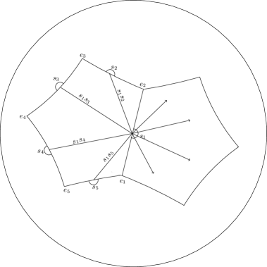
Figura 3: Mobius transformations.

The $5$ singularities are the vertices of the regular hyperbolic polygon. This polygon is the fundamental region of a surface of genus zero whose generators of the Fuchsian group, $\Gamma(S)$, are the elliptic transformations. Since the hyperelliptic curve has genus 2, it follows that the generators of the corresponding Fuchsian subgroup have to be hyperbolic transformations. In order to obtain such generators, the procedure is to fix one of the elliptic transformations and multiply it by each of the remaining elliptic generators. This leads to the four hyperbolic transformations, as shown in the sequence. These four transformations $S_{1}S_{2}$, $S_{1}S_{3}$, $S_{1}S_{4}$, $S_{1}S_{5}$ are the generators of the fundamental region of the bitorus, an eight sided regular hyperbolic polygon.

$$S_{1}S_{2}=\left(\begin{array}[]{ll}1.3090153+0.9510565i&1.209762-0.8789435i\\ 1.209762+0.8789435i&1.3090153-0.9510565i\end{array}\right).$$

$$S_{1}S_{3}=\left(\begin{array}[]{ll}2.4270493+0.5877853i&2.4195239-1.110D-16i\\ 2.4195239+1.110D-16i&2.4270493-0.5877853i\end{array}\right).$$

$$S_{1}S_{4}=\left(\begin{array}[]{ll}2.4270493-0.5877853i&1.957436+1.4221605i\\ 1.957436-1.4221605i&2.4270493+0.5877853i\end{array}\right).$$

$$S_{1}S_{5}=\left(\begin{array}[]{ll}1.3090153-0.9510565i&0.4620879+1.4221605i\\ 0.4620879-1.4221605i&1.3090153+0.9510565i\end{array}\right).$$

By analyzing the tessellation associated with this case, it is possible to see that:

$$\partial f=2g+1\Rightarrow 5=2g+1\Rightarrow g=2.$$

This curve has an associated genus $2$, that is, a bitorus. Therefore, the tessellation associated with Eq. (17) is $\{8,8\}$.

Situation 2: Let us consider the planar algebraic curve $y^{2}=z^{6}-1$. There is an one-to-one correspondence between the six of solutions of $z^{6}-1$ and the values $-2$, $-1$, $0$, $1$, $2$ and $3$, since the roots of the unit divide the circumference into 6 equal parts, as shown in Fig.4.

Figura 4: Singularities of $y^{2}=z^{6}-1$.

In order to follow the same procedure as in Situation 1, it will be presented the associated Fuchsian differential equation, the generators of the Fuchsian group, and the tessellation.

The Fuchsian differential equation is:

$$(z^{6}-3z^{5}-5z+4+15z^{3}+4z^{2}-12z)y^{\prime\prime}+\left[(z^{6}-3z^{5}-5z+4+15z^{3}+4z^{2}-12z)\cdot\left(\frac{2}{z-1}+k_{1}\right)\right]y^{\prime}+$$

$$+[(z^{6}-3z^{5}-5z+4+15z^{3}+4z^{2}-12z)\cdot k_{2}]y=0,\quad k_{1},k_{2}\in\mathbb{C}.$$ (22)

The $6$ singularities are the vertices of the regular hyperbolic polygon. The hyperelliptic curve has genus 2; it follows that the generators of the corresponding Fuchsian subgroup must be hyperbolic transformations. As in the last situation, the procedure is to fix one of the elliptic transformations and multiply it by each of the remaining elliptic generators. This leads to the five hyperbolic transformations as shown in the Fig.5. These five transformations $S_{1}S_{2}$, $S_{1}S_{3}$, $S_{1}S_{4}$, $S_{1}S_{5}$, $S_{1}S_{6}$ are the generators of the fundamental region of the bitorus.

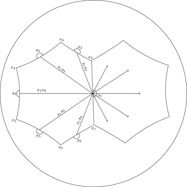
Figura 5: Mobius transformations.

$$S_{1}S_{2}=\left(\begin{array}[]{ll}0.8660252+0.8660254i&0.8264458-0.8264458i\\ 0.8264458+0.8264458i&0.8660252-0.8660254i\end{array}\right).$$

$$S_{1}S_{3}=\left(\begin{array}[]{ll}1.8660252+0.8660254i&1.9553917-0.5239456i\\ 1.9553917+0.5239456i&1.8660252-0.8660254i\end{array}\right).$$

$$S_{1}S_{4}=\left(\begin{array}[]{ll}2.3660252-8.327D-17i&2.2578918+0.6050003i\\ 2.2578918-0.6050003i&2.3660252+8.327D-17i\end{array}\right).$$

$$S_{1}S_{5}=\left(\begin{array}[]{ll}1.8660252-0.8660254i&1.431446+1.431446i\\ 1.431446-1.431446i&1.8660252+0.8660254i\end{array}\right).$$

$$S_{1}S_{6}=\left(\begin{array}[]{ll}0.8660252-0.8660254i&0.3025001+1.1289459i\\ 0.3025001-1.1289459i&0.8660252+0.8660254i\end{array}\right).$$

The tessellation associated with Eq. (22) is $\{10,5\}$.

Note that in the cases analyzed in the Situations 1 and 2, the same genus $g=2$ is obtained by means of two distinct curves $y^{2}=z^{5}-1$ and $y^{2}=z^{6}-1$. Different generators were obtained, which are not isomorphic, but which lead to different tessellations, $\{8,8\}$ for the Situation 1 and $\{10,5\}$ for the Situation 2. These differences found from the computations, associated with the different tessellations, lead to different possibilities of applications and performance analysis in the construction of codes and applications involving the different tessellations related to the same genus (one being denser than the other, for instance).

Another point to be mentioned is that the hyperbolic areas associated with the uniformity regions of the curves $z^{5}-1$ and $z^{6}-1$ are the same, but the number of neighbors is different, resulting in different errors probabilities, in the analysis of the information transmission, since the one that has a greater number of neighbors has a lower error probability.

Finally, let us consider the case associated with the genus 3, organized into two situations, similar to the previous case analyzed.

Situation 3: The corresponding planar algebraic curve is $y^{2}=z^{7}-1$. Note that these seven singularities may be viewed as the vertices of a regular heptagon, as shown in Fig.6.

Figura 6: Singularities of $y^{2}=z^{7}-1$.

Note that there is an one-to-one correspondence between the set of solutions of $z^{7}-1$ and the values $-3$, $-2$, $-1$, $0$, $1$, $2$ and $3$, since the roots of the unit divide the circumference into 7 equal parts. In order to follow the same procedure as in Situation 1 and Situation 2, related to the case associated with the genus 2, it will be presented the associated Fuchsian differential equation, the generators of the Fuchsian group, and the tessellation.

The Fuchsian differential equation is:

$$(z^{7}-14z^{5}+49z^{3}-36z)y^{\prime\prime}+\left[(z^{7}-14z^{5}+49z^{3}-36z)\left(\frac{2}{z+1}+k_{1}\right)\right]y^{\prime}+$$

$$+\left[(z^{7}-14z^{5}+49z^{3}-36z).k_{2}]y\right]=0,\quad k_{1},k_{2}\in\mathbb{C}.$$ (28)

The $7$ singularities are the vertices of the regular hyperbolic polygon. Since the hyperelliptic curve has genus 3, it follows that the generators of the corresponding Fuchsian subgroup have to be hyperbolic transformations. In order to obtain such generators the procedure is to fix one of the elliptic transformations and multiply it by each of the remaining elliptic generators, as show in the Fig. 7. This leads to the six hyperbolic transformations as shown next. These four transformations $S_{1}S_{2}$, $S_{1}S_{3}$, $S_{1}S_{4}$, $S_{1}S_{5}$, $S_{1}S_{6}$, $S_{1}S_{7}$ are the generators of the fundamental region of the tritorus.

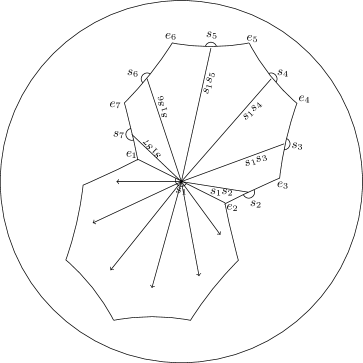
Figura 7: Mobius transformations.

$$S_{1}S_{2}=\left(\begin{array}[]{ll}4.2714376+0.9749279i&3.0675035-0.7001377i\\ 3.0675035+0.7001377i&4.2714376-0.9749279i\end{array}\right).$$

$$S_{1}S_{3}=\left(\begin{array}[]{ll}4.9498855-0.4338837i&3.0675035+2.4462524i\\ 3.0675035-2.4462524i&4.9498855+0.4338837i\end{array}\right).$$

$$S_{1}S_{4}=\left(\begin{array}[]{ll}3.4254268-0.7818315i&-4.441D-16+1.7461148i\\ -4.441D-16-1.7461148i&3.4254268+0.7818315i\end{array}\right).$$

$$S_{1}S_{5}=\left(\begin{array}[]{ll}3.4254268+0.7818315i&1.3651675-1.0886848i\\ 1.3651675+1.0886848i&3.4254268-0.7818315i\end{array}\right).$$

$$S_{1}S_{6}=\left(\begin{array}[]{ll}4.9498855+0.4338837i&3.8251143+0.8730574i\\ 3.8251143-0.8730574i&4.9498855-0.4338837i\end{array}\right).$$

$$S_{1}S_{7}=\left(\begin{array}[]{ll}4.2714376-0.9749279i&1.3651675+2.8347995i\\ 1.3651675-2.8347995i&4.2714376+0.9749279i\end{array}\right).$$

Related to the Eq. (19), we have:

$$\partial f=2g+1\Rightarrow 7=2g+1\Rightarrow g=3.$$

This curve has an associated genus $3$, that is, a tritorus. Therefore, the tessellation associated with Eq. (19) is $\{12,12\}$.

Let us next analyze the case related to the curve $y^{2}=z^{8}-1$, following the same procedure presented in Situations 1, 2 and 3.

Situation 4: For the the curve $y^{2}=z^{8}-1$, there exists a bijective correspondence among the eight solutions of $z^{8}-1$ and the values $-3$, $-2$, $-1$, $0$, $1$, $2$, $3$ and $4$, since the roots of the unit divide the circumference into 8 equal parts, as shown in Fig.8.

The Fuchsian differential equation is given by:

$$(z{}^8-4z{}^7-14z{}^6+56z{}^5+49z{}^4-196z{}^3-36z{}^2+144z)y{}^{\prime \prime }+\left[\right(z{}^8-4z{}^7-14z{}^6+56z{}^5+49z{}^4-196z{}^3-36z{}^2+144z\left)\right]\text{(35)35⋅(2z-1+k1)]y′+[(z8-4z7-14z6+56z5+49z4-196z3-36z2+144z)⋅k2]y=0,k1,k2∈C.}\text{Figura 88Figura 88Singularitiesofy2=z8-1.Figura 8Singul}$$