Bound information in the environment: Environment learns more than it will reveal

Abstract

Quantum systems loose their properties due to information leaking into environment. On the other hand, we perceive the outer world through the environment. We show here that there is a gap between what leaks into the environment and what can be extracted from it. We quantify this gap, using the prominent example of the Caldeira-Leggett model, by demonstrating that information extraction is limited by its own lengthscale, called distinguishability length, larger than the celebrated thermal de Broglie wavelength, governing the decoherence. We also introduce a new integral kernel, called Quantum Fisher Information kernel, complementing the well-known dissipation and noise kernels, and show a type of disturbance-information gain trade-off, similar to the famous fluctuation-dissipation relation. Our results show that the destruction of quantum coherences and indirect observations happen at two different scales with a "gray zone" in between. This puts intrinsic limitations on capabilities of indirect observations.

I Introduction

One of the perpetual questions is if what we perceive is really "out there"? While ontology of quantum mechanics is still a matter of a debate (see e.g. [1, 2, 3]), it is nowadays commonly accepted following the seminal works of Zeh [4] and Zurek [5, 6] that interactions with the environment and resulting decoherence processes lead to an effective emergence of classical properties, like position [7, 8, 9] . It is then usually argued, using idealized pure-state environments, that the decoherence efficiency corresponds directly to the amount of information recorded by the environment (see e.g. [9]). The more environment learns about the system, the stronger it decoheres it. On the other hand, we perceive the outer world by observing the environment and the information content of the latter determines what we see.

Here we show that there is a gap between the two: What the environment learns about the system, as determined by the decohering power, and what can be extracted from it via measurements. Some part of information stays bounded. We show it for physically most relevant thermal environments in the Caldeira-Leggett regime [10], which is the universal choice for high temperature environments, ubiquitous in real-life situations. One of the most emblematic results of the whole decoherence theory states that spatial coherences decay on the lengthscale given by the thermal de Broglie wavelength $\lambda_{dB}$ and on the timescale $t_{dec}\sim\gamma^{-1}(\lambda_{dB}/d)^{2}$, where $d$ is a separation and $\gamma^{-1}$ is related to the relaxation time [11, 10, 12]. We complement this celebrated result by analyzing information extractable from the environment as quantified by the state distinguishability [13]. We show that it is governed by a new lengthscale, which we call distinguishability length, larger than the decoherence length. Thus the resolution with which system’s position can be read-off from the environment is worse than the decoherence resolution. A part of information gained by the environment during the decoherence is bounded in it in the thermal noise, similarly to e.g. bounding a part of thermodynamic energy as thermal energy, unavailable for work, or to bounding quantum entanglement [14]. We obtain the corresponding distinguishability timescale and introduce a new integral kernel, Quantum Fisher Information (QFI) kernel, similar to the well-known noise and dissipation kernels [7, 8, 9] and governing the distinguishability process. The discovery of this phenomenon was possible due to the paradigm change in studies of open quantum systems initiated by quantum Darwinism [15, 16, 17, 18, 19, 20] and Spectrum Broadcast Structures (SBS) [21, 22, 23, 24, 25] programs. They recognize the environment as a carrier of useful information about the system, rather than just the source of noise and dissipation, and study its information content in the context of the quantum-to-classical transition. Some hints on the effect were obtained in earlier studies of SBS, especially in the Quantum Brownian Motion (QBM) model [23], where state distinguishability and its temperature dependence was analyzed, but the limited, numerical character of the studies did not reveal the existence of the distinguishability length and the gap to the decoherence lengthscale. Our results apart from showing intrinsic limitations of indirect observations, also characterize decoherence, which has become one of the key paradigms of modern quantum science [26, 27, 28, 29, 30, 31, 32], from an unusual, little studied perspective of the “receiver’s end”.

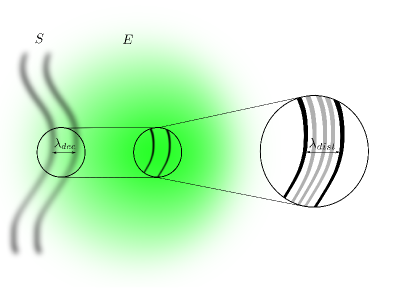
Figure 1: The environment decoheres spatial trajectories of central system at a certain lengthscale $\lambda_{dec}$ (equal to the thermal de Broglie wavelength $\lambda_{dB}$ in the studied example) as a result of dynamical correlation build-up and information leakage into the environment. However not all of that information is accessible. Information retrieval via measurements is limited by its own resolution, the distinguishability length $\lambda_{dist}$, determining how distinguishable are states of the environment corresponding to different states of the central system. Since the distinguishability resolution is worse than the decoherence one, $\lambda_{dist}\gg\lambda_{dec}$, part of the information stays bounded in the environment. Decoherence and distinguishability processes are complementary to each other as reflected by information gain vs. disturbance type of a relation: $\lambda_{dist}\lambda_{dec}=$ const. independent of the state of $E$. The accompanying timescales satisfy $t_{dist}/t_{dec}\sim(\lambda_{dist}/\lambda_{dec})^{2}$, so that reaching a given retrieval resolution takes much longer than the same decoherence resolution.

II Recoilless limit of open quantum systems

Although there exist powerful methods of analysis of quantum open systems, such as the Bloch-Redfield [33, 34] or Davies-Gorini-Kossakowski-Lindblad-Sudarshan [35, 36, 37] equations, they describe the evolution of the central system alone, neglecting the environment completely. This will not tell anything about information acquired by the environment and we instead derive an approximate solution method focusing on the evolution of the environment. Our main object of the study is the partially traced state [21, 22, 23, 25]:

$$\varrho_{S:E_{obs}}={\rm Tr}_{E_{uno}}\varrho_{S:E},$$ (1)

obtained after tracing out only a part of the environment, $E_{uno}$, assumed unobserved. As the first approximation, it is enough to consider the recoiless limit, where the central system $S$ influences the environment $E$ but is massive enough not to feel the recoil. It is a version of the Born-Oppenheimer approximation and the opposite, and less studied, limit to the commonly used Born-Markov approximation [7, 8, 9], where the influence $S\to E$ is completely cut out and is thus useless for our purposes.

We begin following the standard treatment of Feynman and Vernon [38] using path integrals. The full propagator for the system and the environment reads:

$$K_{t}(X,X_{0};x,x_{0})=\int_{\begin{subarray}{l}x(0)=x_{0}\\ x(t)=x\end{subarray}}\mathscr{D}x(t)\int_{\begin{subarray}{l}X(0)=X_{0}\\ X(t)=X\end{subarray}}\mathscr{D}X(t)$$ (2)

$$\times\text{exp}\frac{i}{\hbar}\left\{S_{sys}[X(t)]+S_{env}[x(t)]+S_{int}[X(t),x(t)]\right\}.$$

For a massive enough central system we may neglect the recoil of the environment:

$$\left|\frac{\delta S_{sys}}{\delta X(t)}[X(t)]\right|\gg\left|\frac{\delta S_{int}}{\delta X(t)}[X(t),x(t)]\right|.$$ (3)

and expand the parts containing $X(t)$ around a classical trajectory $X_{cl}(t;X_{0})$ (in what follows we drop the dependence on the initial position $X_{0}$, it will be self-understood), which satisfies the unperturbed equation:

$$\frac{\delta S_{sys}}{\delta X(t)}[X(t)]\approx 0,$$ (4)

due to (3). Following the standard procedure [39], we perform the Gaussian integration around $X_{cl}(t)$:

$$K_{t}\approx\text{e}^{\frac{i}{\hbar}S_{sys}[X_{cl}(t)]}\times$$ (5)

$$\int\mathscr{D}x(t)\text{e}^{\frac{i}{\hbar}S_{env}[x(t)]}\text{e}^{\frac{i}{\hbar}S_{int}[X_{cl}(t),x(t)]}D_{t}(X_{0},X;x(t)),$$

where $D_{t}(X_{0},X;x(t))$ is the van Vleck (semiclassical) determinant [40] for $S_{sys}+S_{int}$. It depends on $x(t)$ through $\delta^{2}S_{int}/\delta X(t)\delta X(t^{\prime})$. This is a quantum leftover of the back-reaction on the central system. We can neglect it and if (3) does not imply it, we assume:

$$\left|\frac{\delta^{2}S_{sys}}{\delta X(t)\delta X(t^{\prime})}[X_{cl}(t)]\right|\gg\left|\frac{\delta^{2}S_{int}}{\delta X(t)\delta X(t^{\prime})}[X_{cl}(t),x(t)]\right|,$$ (6)

which holds trivially e.g. for linearly coupled systems, when $\delta^{2}S_{int}/\delta X(t)\delta X(t^{\prime})=0$. Then $D_{t}(X_{0},X;x(t))$ reduces to the van Vleck propagator for $S$ alone, $D_{t}(X_{0},X)$, and can be pulled out of the integral in (5):

$$K_{t}\approx\text{e}^{\frac{i}{\hbar}S_{sys}[X_{cl}(t)]}D_{t}(X_{0},X)\times$$ (7)

$$\int\mathscr{D}x(t)\text{e}^{\frac{i}{\hbar}S_{env}[x(t)]}\text{e}^{\frac{i}{\hbar}S_{int}[X_{cl}(t),x(t)]}.$$

The first term above is just the semi-classical propagator for the central system alone $K^{sc}_{t}(X,X_{0})$. The remaining path integral in turn, can be reformulated in the operator language as:

$$\int\mathscr{D}x(t)\text{e}^{\frac{i}{\hbar}S_{env}[x(t)]}\text{e}^{\frac{i}{\hbar}S_{int}[X_{cl}(t),x(t)]}\equiv\langle x|\hat{U}_{t}[X_{cl}]|x_{0}\rangle,$$ (8)

where $\hat{U}_{t}[X_{cl}]$ is the driven environment evolution with $X_{cl}(t)$ acting as a classical force:

$$i\hbar\frac{d\hat{U}_{t}}{dt}=\left(\hat{H}_{env}+\hat{H}_{int}[X_{cl}(t)]\right)\hat{U}_{t}.$$ (9)

Thus finally:

$$K_{t}(X,X_{0};x,x_{0})\approx K^{sc}_{t}(X,X_{0})\langle x|\hat{U}_{t}[X_{cl}]|x_{0}\rangle.$$ (10)

This is a sort of a hybrid classical-quantum solution, where the only traces of the quantum character of the central system’s motion are in the determinant $D_{t}(X_{0},X)$ in $K^{sc}_{t}(X,X_{0})$. Assuming a totally uncorrelated initial state $\varrho(0)=\varrho_{0S}\otimes\bigotimes_{k}\varrho_{0k}$ and tracing out the unobserved part of the environment $E_{uno}$, we obtain the desired solution in a form of partial matrix elements:

$$\langle X^{\prime}|\varrho_{S:E_{obs}}(t)|X\rangle\approx$$

$$\int\int dX_{0}dX^{\prime}_{0}\langle X^{\prime}_{0}|\varrho_{0S}|X_{0}\rangle K^{sc}_{t}(X,X_{0})^{*}K^{sc}_{t}(X^{\prime},X^{\prime}_{0})$$

$$\times F[X_{cl}(t),X^{\prime}_{cl}(t)]\bigotimes_{k\in E_{obs}}\hat{U}^{k}_{t}[X_{cl}]\varrho_{0k}\hat{U}^{k}_{t}[X^{\prime}_{cl}]^{\dagger}.$$ (11)

Here $X_{cl}(0)=X_{0}$, $X_{cl}(t)=X$, $X^{\prime}_{cl}(0)=X^{\prime}_{0}$, $X^{\prime}_{cl}(t)=X^{\prime}$ and:

$$F[X_{cl}(t),X^{\prime}_{cl}(t)]\equiv\prod_{k\in E_{uno}}{\rm Tr}\left(\hat{U}^{k}_{t}[X^{\prime}_{cl}]^{\dagger}\hat{U}^{k}_{t}[X_{cl}]\varrho_{0k}\right)$$ (12)

is the influence functional [38, 39] due to $E_{uno}$. This is a hybrid, classical-quantum solution, where the central system behaves as an undamped oscillator and drives the environment.

In what follows we will specify to one of the paradigmatic models of open quantum systems, Quantum Brownian Motion model (see e.g. [41, 42, 43]), as an example. It is described by Lagrangeans:

$$L_{sys}=\frac{M\dot{X}^{2}}{2}-\frac{M\Omega^{2}X^{2}}{2}$$ (13)

$$L_{env}=\sum_{k}\left(\frac{m_{k}\dot{x}_{k}^{2}}{2}-\frac{m_{k}\omega_{k}^{2}x_{k}^{2}}{2}\right)=\sum_{k}L_{k}$$ (14)

$$L_{int}=-X\sum_{k}C_{k}x_{k}$$ (15)

and the corresponding actions. The no-recoil condition (3) will be satisfied when the influence of each environmental oscillator can be neglected, which is controlled by a dimensionless quantity:

$$\frac{C_{k}}{M\Omega^{2}}\ll 1,$$ (16)

while (6) is trivial due to the linearity in $X$. The unperturbed classical trajectories are then given by (outside of the focal points):

$$X_{cl}(\tau)=X_{0}\cos\Omega\tau+\frac{X-X_{0}\cos\Omega t}{\sin\Omega t}\sin\Omega\tau.$$ (17)

As a side remark, (11) can be also obtained in the following way. Forgetting for a moment the evolution of the environment, the central system is a forced harmonic oscillator with a well-known solution for the propagator [38]. It is determined by the action:

$$S[x(t)]=\frac{M\Omega}{2\sin\Omega t}\big{[}(X^{2}+X_{0}^{2})\cos\Omega t-2XX_{0}\big{]}+$$

$$\frac{1}{\sin\Omega t}\sum_{k}C_{k}\int_{0}^{t}d\tau\left[X\sin\Omega\tau+X_{0}\sin\Omega(t-\tau)\right]x_{k}(\tau)$$

$$-\frac{\Omega}{\sin\Omega t}\sum_{k,l}\frac{C_{k}C_{l}}{M\Omega^{2}}\int_{0}^{t}d\tau\int_{0}^{\tau}d\tau^{\prime}\sin\Omega\tau^{\prime}\sin\Omega(t-\tau)$$

$$\times x_{k}(\tau)x_{l}(\tau^{\prime}).$$ (18)

Neglecting the last term and using the resulting action to construct the propagator for the global state, we obtain (11).

The influence functional has been first calculated in [38] for the physically most relevant situation of the thermal environments. We quote the well known formulas for completeness [38, 10, 7, 8]:

$$F[X_{cl}(t),X^{\prime}_{cl}(t)]=$$

$$\text{exp}\left\{-\frac{1}{\hbar}\int_{0}^{t}d\tau\int_{0}^{\tau}d\tau^{\prime}\Delta(\tau)\nu(\tau-\tau^{\prime})\Delta(\tau^{\prime})\right\}\times$$ (19)

$$\text{exp}\left\{-\frac{i}{\hbar}\int_{0}^{t}d\tau\int_{0}^{\tau}d\tau^{\prime}\Delta(\tau)\eta(\tau-\tau^{\prime})\bar{X}_{cl}(\tau^{\prime})\right\},$$ (20)

where:

$$\Delta(\tau)\equiv X_{cl}(\tau)-X^{\prime}_{cl}(\tau)$$

$$=\Delta X_{0}\frac{\sin[\Omega(t-\tau)]}{\sin\Omega t}+\Delta X\frac{\sin\Omega\tau}{\sin\Omega t},$$ (21)

$$\bar{X}_{cl}(\tau)\equiv\frac{1}{2}\left[X_{cl}(\tau)+X^{\prime}_{cl}(\tau)\right],$$ (22)

$\Delta X_{0}\equiv X_{0}-X_{0}^{\prime}$, $\Delta X=X-X^{\prime}$, and

$$\nu(\tau)\equiv\int d\omega J_{\perp}(\omega)\mathrm{cth}\left(\frac{\hbar\omega\beta}{2}\right)\cos\omega\tau,$$ (23)

$$\eta(\tau)\equiv\int d\omega J_{\perp}(\omega)\sin\omega\tau$$ (24)

are the noise and the dissipation kernels respectively. Here $\beta=1/(k_{B}T)$ and $J_{\perp}(\omega)\equiv\sum_{k\in E_{uno}}\frac{C_{k}^{2}}{2m_{k}\omega_{k}}\delta(\omega-\omega_{k})$ is the spectral density corresponding to the unobserved part of the environment.

III Distinguishability of local states and Quantum Fisher Information kernel

To understand what information about $S$ is available locally in the the environment, we need the local states of each fragment $E_{k}$:

$$\varrho_{E_{k}}(t)={\rm Tr}_{E_{1}\dots\hat{E}_{k}\dots}{\rm Tr}_{S}\varrho_{S:E_{obs}}$$ (25)

$$={\rm Tr}_{E_{1}\dots\hat{E}_{k}\dots}\int dX\langle X|\varrho_{S:E_{obs}}|X\rangle$$ (26)

The calculation is presented in Appendix A and relies on the no-recoil condition (16). The result is:

$$\varrho_{E_{k}}(t)\approx$$

$$\int dX_{0}p(X_{0}){\rm Tr}_{E_{1}\dots\hat{E}_{k}\dots}\bigotimes_{j\in E_{obs}}\hat{U}^{j}_{t}[X^{0}_{cl}]\varrho_{0j}\hat{U}^{j}_{t}[X^{0}_{cl}]^{\dagger}$$

$$\equiv\int dX_{0}p(X_{0})\varrho^{k}_{t}[X^{0}_{cl}],$$ (27)

and similarly if several $E_{k}$’s are considered. We have defined conditional states:

$$\varrho^{k}_{t}[X_{cl}]\equiv\hat{U}^{k}_{t}[X_{cl}]\varrho_{0k}\hat{U}^{k}_{t}[X_{cl}]^{\dagger},$$ (28)

$p(X_{0})$ is the initial distribution:

$$p(X_{0})\equiv\langle X_{0}|\varrho_{0S}|X_{0}\rangle,$$ (29)

and $X^{0}_{cl}$ is the classical trajectory with the endpoint $0$:

$$X^{0}_{cl}(0)=X_{0},\ X^{0}_{cl}(t)=0.$$ (30)

The operators $\hat{U}^{k}_{t}[X_{cl}]$ satisfy (9), which takes the form:

$$i\hbar\frac{d\hat{U}^{k}_{t}}{dt}=\left(\hat{H}_{k}+C_{k}X_{cl}(t)\hat{x}_{k}\right)\hat{U}^{k}_{t},$$ (31)

and the solution in the interaction picture is given by the displacement operator:

$$\hat{U}^{k}_{t}[X_{cl}]=e^{i\zeta_{k}(t)}D\left(-\frac{iC_{k}}{\sqrt{2\hbar m_{k}\omega_{k}}}\int_{0}^{t}d\tau e^{i\omega_{k}\tau}X_{cl}(\tau)\right),$$ (32)

where $\zeta_{k}(t)$ is an unimportant phase factor and $D(\alpha)\equiv\exp(\alpha a^{\dagger}-\alpha^{*}a)$. Thus, the local states seen by each of the environmental observers are mixtures of forced oscillator states (28), forced along classical trajectories (30). The states are parametrized by the central system’s initial position $X_{0}$ (cf. [23]), spread with the probability $p(X_{0})$.

The information content of the fragment $E_{k}$ is determined by the distinguishability of the local states $\varrho^{k}_{t}[X_{cl}]$ for different trajectories. We will consider a general $X_{cl}(\tau)$, which can later be specified to $X^{0}_{cl}(\tau)$. Among the available distinguishability measures [13], a particularly convenient one is the generalized overlap $B(\varrho,\sigma)\equiv{\rm Tr}\sqrt{\sqrt{\varrho}\sigma\sqrt{\varrho}}$. It provides a lower (and upper) bound for such operational quantities as the probability of error and to the quantum Chernoff information [44] and is a good compromise between computability and a clear operational meaning. We define:

$$B_{k}[\Delta,t]\equiv B(\varrho^{k}_{t}[X_{cl}],\varrho^{k}_{t}[X^{\prime}_{cl}])$$ (33)

(from (28) that $B$ depends only on the trajectories difference). Using (32) and the calculation of the overlap for thermal $\varrho_{0k}$ [23], we find:

$$B_{k}[\Delta,t]=$$ (34)

$$\mathrm{exp}\left\{-\frac{C_{k}^{2}}{4\hbar m_{k}\omega_{k}}\mathrm{th}\left(\frac{\hbar\omega_{k}\beta}{2}\right)\left|\int_{0}^{t}d\tau\mathrm{e}^{i\omega_{k}\tau}\Delta(\tau)\right|^{2}\right\}.$$

A single environmental mode may be either inaccessible or carry vanishingly small amount of useful information. In order to decrease the discrimination error, it is therefore more reasonable to combine the observed modes into groups called macrofractions [21], which are fragments scaling with the total number of observed modes $N_{obs}$. Since there are no direct interactions among the environment modes here, the states of macrofractions are products (cf. (27)): $\varrho^{mac}_{t}[X_{cl}]\equiv\bigotimes_{k\in mac}\varrho^{k}_{t}[X_{cl}]$. The generalized overlap factorizes w.r.t. the tensor product, so there is no quantum metrological advantage [45], but still there is a classical advantage [21] (the possibility of a quantum advantage will be discussed elsewhere):

$$B_{mac}[\Delta,t]\equiv B(\varrho^{mac}_{t}[X_{cl}],\varrho^{mac}_{t}[X^{\prime}_{cl}])=\prod_{k\in mac}B_{k}[\Delta,t]$$

$$=\mathrm{exp}\left\{-\frac{1}{\hbar}\int_{0}^{t}d\tau\int_{0}^{\tau}d\tau^{\prime}\Delta(\tau)\phi(\tau-\tau^{\prime})\Delta(\tau^{\prime})\right\},$$ (35)

where we introduced the spectral density describing the macrofraction $J_{mac}(\omega)\equiv\sum_{k\in mac}\frac{C_{k}^{2}}{2m_{k}\omega_{k}}\delta(\omega-\omega_{k})$ and a new integral kernel:

$$\phi(\tau)\equiv\int_{0}^{\infty}d\omega J_{mac}(\omega)\mathrm{th}\left(\frac{\hbar\omega\beta}{2}\right)\cos\omega\tau,$$ (36)

which we call quantum Fisher information kernel. Note that, quite surprisingly, the QFI kernel and the overlap (35) have almost identical structure to the noise kernel (23) and the real part of the influence functional (19), with the only difference being in the reversed temperature dependence [23, 46]. It can be intuitively understood by recalling that (19) is responsible for decoherence and in this model the higher the temperature the more efficient the decoherence. On the other hand, higher temperature means the environment is more noisy and hence less able to store information about the central system.

The name QFI kernel comes from the following observation. Let us consider the encoding of the variable $X_{0}$ in the thermal states of the environment by means of the interaction Hamiltonian only:

$$\varrho_{k}(X)\equiv\mathrm{e}^{-i/\hbar X_{0}C_{k}\hat{x}_{k}}\varrho_{0k}\mathrm{e}^{i/\hbar X_{0}C_{k}\hat{x}_{k}}.$$ (37)

If we calculate the QFI associated with such an encoding (see e.g. [47]) we obtain:

$$\mathcal{F}(\varrho_{0k};\hat{x}_{k})=\frac{2C_{k}^{2}}{\hbar m_{k}\omega_{k}}\mathrm{th}\left(\frac{\beta\hbar\omega_{k}}{2}\right),$$ (38)

which is proportional to the integrand of (36). This comes of no surprise as it is well known that QFI is the infinitesimal form of the generalized overlap.

The definition of what is macrofraction is a bit subtle in the continuum limit. There are at least two general possibilities [48]: Multiply the environments or divide the frequency spectrum. In the first case, one assumes that the traced over and all the observed macrofractions are so big that can be to a good degree described by own, full-spectrum spectral densities. This corresponds to an effective multiplication of the environment–each environment exists in several copies, one of which is neglected and the rest observed. Physically, it corresponds to e.g. an observation using wide-band detectors as the full frequency spectrum is under the observation. The second scenario consists in a division of the frequency spectrum into intervals each of which defines the observed fraction and corresponds to a narrow-band detection.

We will use the first approach here, since we want a fair comparison of the decohering power and the information content of the same piece of the environment. We assume that each macrofraction is described by the same Lorenz-Drude spectral density, which is the most popular choice in the model [7, 8, 9]:

$$J(\omega)=\frac{2M\gamma}{\pi}\omega\frac{\Lambda^{2}}{\Lambda^{2}+\omega^{2}},$$ (39)

where $\Lambda$ is the high-frequency cutoff and $\gamma$ is the effective coupling strength.

IV The information gap

The noise and the QFI kernels are in general complicated functions and for our demonstration it is enough to use the popular Caldeira-Leggett regime [10, 9], which is the high-temperature, high-cutoff limit:

$$k_{B}T/\hbar\gg\Lambda\gg\Omega.$$ (40)

The behavior of the influence functional in this limit is emblematic to the whole decoherence theory and can be obtained e.g. by approximating $\text{cth}x\approx x^{-1}$ in the noise kernel (23) and then using $\Lambda e^{-\Lambda\tau}\approx\delta(\tau)$ valid for $\tau\gg\Lambda^{-1}$. This leads to the celebrated result [11, 10, 12, 8]:

$$\Big{|}F[X_{cl}(t),X^{\prime}_{cl}(t)]\Big{|}\approx\mathrm{exp}\left[-\frac{\gamma}{\lambda_{dB}^{2}}\int_{0}^{t}d\tau\Delta(\tau)^{2}\right],$$ (41)

where

$$\lambda_{dB}^{2}=\frac{\hbar^{2}}{2Mk_{B}T}$$ (42)

is the thermal de Broglie wavelength, stating that the decoherence becomes efficient at lengths above $\lambda_{dB}$ and for times larger than the decoherence time [12]:

$$t_{dec}=\frac{1}{\gamma}\left(\frac{\lambda_{dB}}{d}\right)^{2},$$ (43)

where $d$ is a given separation and $\gamma^{-1}$ is related to the relaxation time.

Let us study the QFI kernel in the similar way. Approximating $\text{th}x\approx x$ in (36), we obtain (cf. Appendix B for Matsubara series analysis):

$$\phi(\tau)\underset{\hbar\Lambda\beta\ll 1}{\approx}\frac{\gamma M\hbar\beta\Lambda^{2}}{\pi}\int_{0}^{\infty}d\omega\frac{\omega^{2}}{\omega^{2}+\Lambda^{2}}\cos(\omega\tau)$$ (44)

$$=\frac{\gamma M\hbar\beta\Lambda^{2}}{\pi}\left(\int_{0}^{\infty}d\omega\cos(\omega\tau)-\Lambda^{2}\int_{0}^{\infty}d\omega\frac{\cos(\omega\tau)}{\omega^{2}+\Lambda^{2}}\right)$$ (45)

$$=\gamma M\hbar\beta\left(\Lambda^{2}\delta(\tau)-\frac{1}{2}\Lambda^{3}e^{-\Lambda|\tau|}\right).$$ (46)

We define $f(\tau)\equiv\Lambda e^{-\Lambda\tau}$ for $\tau>0$ so that $\Lambda^{3}e^{-\Lambda(\tau-\tau^{\prime})}=d^{2}/d\tau^{\prime 2}f(\tau-\tau^{\prime})$. We can then calculate the integral with the second term of (46) integrating by parts two times:

$$\int_{0}^{\tau}d\tau^{\prime}\Lambda^{3}e^{-\Lambda(\tau-\tau^{\prime})}\Delta(\tau^{\prime})=\int_{0}^{\tau}d\tau^{\prime}\ddot{f}(\tau-\tau^{\prime})\Delta(\tau^{\prime})$$ (47)

$$=\dot{f}(0_{+})\Delta(\tau)-\dot{f}(\tau)\Delta(0)-f(0)\dot{\Delta}(\tau)+f(\tau)\dot{\Delta}(0)$$ (48)

$$+\int_{0}^{\tau}d\tau^{\prime}f(\tau-\tau^{\prime})\ddot{\Delta}(\tau^{\prime}),$$ (49)

here the dot means $d/d\tau^{\prime}$, so that $\dot{f}(0_{+})=+\Lambda^{2}$. In the large cut-off limit it is justified to assume $\tau\gg\Lambda^{-1}$, i.e. we consider timescale much larger than the one set by the cut-off, similarly as it is done analyzing the influence functional [10]. Then the boundary terms containing $f(\tau)$ and $\dot{f}(\tau)$ can be neglected and moreover we can substitute $f(\tau)\approx\delta(\tau)$ in the last integral to obtain:

$$\int_{0}^{\tau}d\tau^{\prime}\Lambda^{3}e^{-\Lambda|\tau-\tau^{\prime}|}\Delta(\tau^{\prime})\underset{\Lambda\tau\gg 1}{\approx}\Lambda^{2}\Delta(\tau)-\Lambda\dot{\Delta}(\tau)+\ddot{\Delta}(\tau)$$ (50)

$$=\Lambda^{2}\Delta(\tau)-\Lambda\Omega\Delta\left(\tau+\frac{\pi}{2\Omega}\right)-\Omega^{2}\Delta(\tau)$$ (51)

$$\underset{\Lambda\gg\Omega}{\approx}\Lambda^{2}\Delta(\tau),$$ (52)

where we used $\dot{\Delta}(\tau)=\Omega\Delta(\tau+\pi/2\Omega)$ and $\ddot{\Delta}(\tau)=-\Omega^{2}\Delta(\tau)$ and neglected the $\Omega$-terms because $\Lambda\gg\Omega$. More generally, $\dot{\Delta}(\tau)$, $\ddot{\Delta}(\tau)$ are inverse proportional to the system’s evolution time-scale, which is the slowest time-scale, and hence those terms can be omitted compared to the $\Lambda^{2}$ term. Using (52) and (46) we can finally calculate (35):

$$B[\Delta,t]\approx\mathrm{exp}\left[-\frac{\gamma}{\lambda^{2}_{dist}}\int_{0}^{t}d\tau\Delta(\tau)^{2}\right],$$ (53)

This is our main result. The distinguishability process defines its own lengthscale – the distinguishability length:

$$\lambda_{dist}^{2}\equiv\frac{2k_{B}T}{M\Lambda^{2}}=\frac{\hbar}{M\Lambda}\left(\frac{2k_{B}T}{\hbar\Lambda}\right)$$ (54)

and the associated distinguishability timescale:

$$t_{dist}=\frac{1}{\gamma}\left(\frac{\lambda_{dist}}{d}\right)^{2},$$ (55)

similarly to (42),(43). Surprisingly, (54) does not depend on $\hbar$ in the leading order and is the lengthscale at which the energy of the "cut-off oscillator" of mass $M$ and frequency $\Lambda$ equals the thermal energy: $M\Lambda^{2}\lambda_{dist}^{2}/2=k_{B}T$. The cut-off dependence can be understood as it defines the shortest lengthscale in the environment: (54) can be expressed as the characteristic length of the cut-off oscillator , $\sqrt{\hbar/M\Lambda}$, rescaled by the ratio of the thermal energy to the cut off energy, $\sqrt{2k_{B}T/\hbar\Lambda}$. Of course the higher order terms in the $\text{th}(\hbar\beta\omega/2)$ expansion in (35),(36) will contribute $O(\hbar^{2})$ terms to (54). There is clearly a competition in (54) between the temperature $T$, which degrades the discriminating ability of the environment and the cut-off frequency $\Lambda$ which increases it. The relative difference between the two lengthscales:

$$\frac{\lambda_{dist}-\lambda_{dB}}{\lambda_{dB}}\approx 2\frac{k_{B}T}{\hbar\Lambda}\gg 1,$$ (56)

shows that there is a “resolution gap” between the decoherence and the distinguishability resolutions [49]. The environment decoheres the system at shorter lengthscales than those at which the position information can be extracted from it, i.e. a part of information stays bounded in the environment. The timescales are separated even stronger:

$$\frac{t_{dist}}{t_{dec}}=4\left(\frac{k_{B}T}{\hbar\Lambda}\right)^{2},$$ (57)

meaning the distinguishability process takes much longer time than the decoherence for the same separation. This is in accord with the earlier results for generic finite dimensional systems [50]. For molecular environments $\Lambda\sim 10^{13}$Hz and at $T\sim 300$K, $\lambda_{dist}/\lambda_{dec}\sim 10$, $t_{dist}/t_{dec}\sim 100$, which is still orders of magnitude shorter for macroscopic bodies than typical relaxation times [12].

V Disturbance vs. Information Gain

As a by-product we obtain a type of information gain vs. disturbance relation (see e.g. [51]), disturbance being represented by the decoherence efficiency, in a form of a lengthscale complementarity relation:

$$\lambda_{dB}\lambda_{dist}=\frac{\hbar}{M\Lambda}.$$ (58)

The right hand side does not depend on the state of the environment (encoded in the temperature) and is the square of the characteristic length of the cut-off oscillator. More generally, we can write the following formal relations between the QFI, noise, and dissipation kernels, true for thermal environments:

$$\hat{\phi}(\omega)=\hat{\nu}(\omega)\text{th}^{2}\left(\frac{\hbar\omega\beta}{2}\right),$$ (59)

$$\hat{\phi}(\omega)=i\hat{\eta}(\omega)\text{th}\left(\frac{\hbar\omega\beta}{2}\right),$$ (60)

and resembling the celebrated fluctuation-dissipation relations [52, 42, 53] $\hat{\nu}(\omega)=i\hat{\eta}(\omega)\text{cth}(\hbar\omega\beta/2)$, where the hat denotes the Fourier transform. Those intriguing relations will be studied elsewhere.

VI Conclusions

We have shown here, using the celebrated model of Caldeira and Leggett as an example, that there is an information gap between what environment learns, decohering the system, and what can be extracted from it via measurements, i.e. some information stays bounded in the environment. For that, we have developed a series of rather non-trivial and non-standard tools, including a path integral recoiless limit, a hybrid quantum-classical extended state solution (11), and Quantum Fisher information kernel. Our results uncover the existence of a new lengthscale, determining information content of the environment and complementary to the celebrated thermal de Broglie decoherence lengthscale.

The unorthodox point of view taken here, i.e. that of the environment instead of the the central system, has been motivated by the modern developments of the decoherence theory [15, 21, 17], explaining the apparent objectivity of the macroscopic world through redundantly stored information in the environment. From this perspective, the solution (11) can approximate an SBS state, storing an objective position of the central system, in the semi-classical approximation. We hypothesize that approach to objectivity is possible only in such a limit, when the central system is macroscopic enough, making objectivity a macroscopic phenomenon.

We acknowledge the support by Polish National Science Center (NCN) (Grant No. 2019/35/B/ST2/01896). JKK acknowledges discussions with J. Tuziemski in the early stages of the work.

Appendix A Calculation of the trace over the system

Here we calculate the trace over the central system $S$. We first assume for simplicity only one observed environment and one unobserved. Generalization to multiple environments in both groups will be obvious and we present it at the end. The main idea is to rewrite the integral (26) such that the no-recoil condition (16) can be used. First, we take matrix elements w.r.t. the environment and comeback from the operator form of (11) to the path integral one, using (8):

$$\int dX\langle X;x^{\prime}|\varrho_{S:E_{obs}}|X;x\rangle=$$

$$\int dX_{0}dX_{0}^{\prime}dx_{0}dx^{\prime}_{0}\langle X^{\prime}_{0}|\varrho_{0S}|X_{0}\rangle\langle x^{\prime}_{0}|\varrho_{0E}|x_{0}\rangle\int dXK^{sc}_{t}(X,X_{0})^{*}K^{sc}_{t}(X,X^{\prime}_{0})F[X_{cl},X^{\prime}_{cl}]$$ (61)

$$\times\int\mathscr{D}x\mathscr{D}x^{\prime}\exp\frac{i}{\hbar}\Big{(}S_{env}[x]-S_{env}[x^{\prime}]+S_{int}[X_{cl},x]-S_{int}[X^{\prime}_{cl},x^{\prime}]\Big{)}$$ (62)

Above due to the tracing (26), classical trajectories have the same endpoints $X_{cl}(t)=X_{cl}^{\prime}(t)=X$, and $x(0)=x_{0}$, $x(t)=x$ and similarly for $x^{\prime}(\tau)$. Let us analyze the above expression term by term. It is well known that the semiclassical propagator $K^{sc}_{t}(X,X_{0})$ for harmonic oscillator is equal to the full quantum one. We thus have:

$$K^{sc}_{t}(X,X_{0})^{*}K^{sc}_{t}(X,X^{\prime}_{0})=$$ (63)

$$\frac{M\Omega}{2\pi\hbar|\sin\Omega t|}e^{\frac{iM\Omega}{2\hbar\sin\Omega t}\big{[}(X_{0}^{\prime 2}-X_{0}^{2})\cos\Omega t+2X\Delta X_{0}\big{]}}.$$ (64)

There are $X$-dependent and $X$-independent parts.

The influence functional may be written using path integrals as [39]:

$$F[X_{cl},X^{\prime}_{cl}]=\int d\tilde{y}dy_{0}dy^{\prime}_{0}\int\mathscr{D}y\mathscr{D}y^{\prime}\langle y^{\prime}_{0}|\tilde{\varrho}_{0E}|y_{0}\rangle$$

$$\times e^{\frac{i}{\hbar}\big{(}S_{env}[y]-S_{env}[y^{\prime}]+S_{int}[X_{cl},y]-S_{int}[X^{\prime}_{cl},y^{\prime}]\big{)}},$$ (65)

where $\tilde{\varrho}_{0E}$ is the initial state of the unobserved part of the environment $E_{uno}$, which can be different from the initial state of the observed part $E_{obs}$, $\varrho_{0E}$ in (61). The boundary conditions are $y(0)=y_{0}$, $y^{\prime}(0)=y^{\prime}_{0}$, $y(t)=y^{\prime}(t)=\tilde{y}$. The generalization to multiple unobserved environments is straightforward – the combined influence functional will be a product over $j\in E_{uno}$ of the terms (65) for each mode $j$ with $\varrho_{0j}$ initial state, $F=\prod_{j\in E_{uno}}F_{j}$

The terms of the form $S_{env}[x]-S_{env}[x^{\prime}]$, appearing both in (62) and (65), do not depend on the integration variable $X$ and thus can pulled in from of the integral over $X$. The interaction terms $S_{int}[X_{cl},y]-S_{int}[X^{\prime}_{cl},y^{\prime}]$ from (62), (65) will have both $X$-dependent and $X$-independent parts. To separate them, let us rewrite the classical trajectory (17) and simplify the notation:

$$X_{cl}(\tau)=X_{0}\cos\Omega\tau\left[1-\frac{\sin\Omega\tau}{\sin\Omega t}\right]+X\frac{\sin\Omega\tau}{\sin\Omega t}$$ (66)

$$\equiv X_{0}a(\tau)+X\frac{\sin\Omega\tau}{\sin\Omega t}.$$ (67)

Then it is easy to see that (cf. (15)):

$$S_{int}[X_{cl},x]-S_{int}[X^{\prime}_{cl},x^{\prime}]=$$

$$-C\int_{0}^{t}d\tau a(\tau)\left[X_{0}x(\tau)-X_{0}^{\prime}x^{\prime}(\tau)\right]$$ (68)

$$-\frac{CX}{\sin\Omega t}\int_{0}^{t}d\tau\sin\Omega\tau\left[x(\tau)-x^{\prime}(\tau)\right]$$ (69)

We now combine the $X$-dependent factors from (62),(64),(65) and integrate them over $X$:

$$\frac{M\Omega}{2\pi\hbar|\sin\Omega t|}\int dX\exp\Bigg{\{}\frac{iX}{\hbar\sin\Omega t}\bigg{[}M\Omega\Delta X_{0}-C\int_{0}^{t}d\tau\sin\Omega\tau\left[x(\tau)-x^{\prime}(\tau)+y(\tau)-y^{\prime}(\tau)\right]\bigg{]}\Bigg{\}}$$ (70)

$$=\frac{M\Omega}{2\pi\hbar|\sin\Omega t|}\int dX\exp\Bigg{\{}\frac{iXM\Omega^{2}}{\hbar\sin\Omega t}\bigg{[}\frac{\Delta X_{0}}{\Omega}-\frac{C}{M\Omega^{2}}\int_{0}^{t}d\tau\sin\Omega\tau\left[x(\tau)-x^{\prime}(\tau)+y(\tau)-y^{\prime}(\tau)\right]\bigg{]}\Bigg{\}}$$ (71)

$$\approx\frac{M\Omega}{2\pi\hbar|\sin\Omega t|}\int dX\exp\bigg{(}\frac{iXM\Omega\Delta X_{0}}{\hbar\sin\Omega t}\bigg{)}=\delta\left(\Delta X_{0}\right),$$ (72)

where in the crucial step we used the recoilless condition (16) and neglected the action integral. We can now comeback to the main integral (61,62). The delta function (72) forces the trajectories $X_{cl}(\tau)$ and $X_{cl}(\tau)$ to be equal as it forces $X_{0}=X_{0}^{\prime}$ (the endpoints are the same in this calculation as we are calculating the trace over $X$). This immediately forces the influence functional (65) to be equal to one since:

$$F[X_{cl},X_{cl}]={\rm Tr}\left(\hat{U}_{t}[X_{cl}]\tilde{\varrho}_{0E}\hat{U}_{t}[X_{cl}]^{\dagger}\right)=1$$ (73)

The $X$-independent part of (64) will be equal to one too, since $X_{0}^{\prime 2}-X^{2}_{0}=0$. We are thus left with the following integral:

$$\int dX\langle X;x^{\prime}|\varrho_{S:E_{obs}}|X;x\rangle=\int dX_{0}p(X_{0})\int dx_{0}dx^{\prime}_{0}\langle x^{\prime}_{0}|\varrho_{0E}|x_{0}\rangle$$ (74)

$$\times\int\mathscr{D}x\mathscr{D}x^{\prime}\exp\frac{i}{\hbar}\Big{(}S_{env}[x]-S_{env}[x^{\prime}]-C\int_{0}^{t}d\tau a(\tau)\left[X_{0}x(\tau)-X_{0}^{\prime}x^{\prime}(\tau)\right]\Big{)}$$ (75)

$$=\int dX_{0}p(X_{0})\int dx_{0}dx^{\prime}_{0}\langle x^{\prime}_{0}|\varrho_{0E}|x_{0}\rangle\int\mathscr{D}x\mathscr{D}x^{\prime}e^{\frac{i}{\hbar}\big{(}S_{env}[x]+S_{int}[X^{0}_{cl},x]-S_{env}[x^{\prime}]-S_{int}[X^{0}_{cl},x^{\prime}]\big{)}}$$ (76)

$$=\int dX_{0}p(X_{0})\langle x^{\prime}|U_{t}[X^{0}_{cl}]\varrho_{0E}U_{t}[X^{0}_{cl}]^{\dagger}|x\rangle,$$ (77)

where in (76) we came back to the operator picture using (8, 9) and

$$p(X_{0})\equiv\langle X_{0}|\varrho_{0S}|X_{0}\rangle$$ (78)

is the initial distribution of the central system’s position. Above, $X^{0}_{cl}$ is the classical trajectory with the endpoint $0$:

$$X^{0}_{cl}(0)=X_{0},\ X^{0}_{cl}(t)=0.$$ (79)

It appears by comparing the action integral in the exponent of (75) to (67) with $X=0$. Having the result (77) for a single degree of freedom of the observed environment, we can now apply it to the initial task with multiple environments. Performing the above calculations for each degree of freedom $j$ we finally obtain:

$$\varrho_{E_{k}}(t)={\rm Tr}_{E_{1}\dots\hat{E}_{k}\dots}\int dX\langle X|\varrho_{S:E_{obs}}|X\rangle\approx$$ (80)

$$\int dX_{0}p(X_{0}){\rm Tr}_{E_{1}\dots\hat{E}_{k}\dots}\bigotimes_{j\in E_{obs}}\hat{U}^{j}_{t}[X^{0}_{cl}]\varrho_{0j}\hat{U}^{j}_{t}[X^{0}_{cl}]^{\dagger}$$

$$=\int dX_{0}p(X_{0})\hat{U}^{k}_{t}[X^{0}_{cl}]\varrho_{0k}\hat{U}^{k}_{t}[X^{0}_{cl}]^{\dagger}$$ (81)

$$\equiv\int dX_{0}p(X_{0})\varrho^{k}_{t}[X^{0}_{cl}],$$ (82)

where the approximation signalizes that we have used the no-recoil condition (16) and we have defined

$$\varrho^{k}_{t}[X_{cl}]\equiv\hat{U}^{k}_{t}[X_{cl}]\varrho_{0k}\hat{U}^{k}_{t}[X_{cl}]^{\dagger}.$$ (83)

Appendix B Matsubara representation of the QFI kernel

Just like in the case of the noise kernel [7], one can derive a formal analytic expression for the QFI kernel using the fermionic Matsubara representation [54]:

$$\mathrm{th}\left(\frac{\beta\hbar\omega}{2}\right)=\frac{4}{\beta\hbar\omega}\sum_{n=0}^{\infty}\frac{1}{1+(\nu_{n}/\omega)^{2}},$$ (84)

with fermionic frequencies

$$\nu_{n}=\frac{(2n+1)\pi}{\hbar\beta}.$$ (85)

Substituting this into the QFI definition and integrating term by term, we find:

$$\phi(\tau)=\frac{4M\gamma\Lambda}{\hbar\beta}\sum_{n=0}^{\infty}\frac{e^{-\Lambda|\tau|}-(\nu_{n}/\Lambda)\mathrm{e}^{-\nu_{n}|\tau|}}{1-(\nu_{n}/\Lambda)^{2}},$$ (86)

which looks identical to the expansion of the noise kernel $\nu(\tau)$ [7], except that instead of the bosonic frequencies $\nu_{n}=2n\pi/(\hbar\beta)$ we now have the fermionic (85). In particular now $\nu_{0}=\pi/(\hbar\beta)\neq 0$ so that $\nu_{n}/\Lambda\gg 1$ for any $n$, including $n=0$. This complicates the analysis compared to the bosonic case, describing the influence functional, as there is now an interplay between $\Lambda$, $\nu_{0}$, and $\tau$. The double integral in (35), which we denote by $\Phi[\Delta,t]$:

$$\Phi[\Delta,t]\equiv\int^{t}_{0}d\tau\int^{\tau}_{0}d\tau^{\prime}\Delta(\tau)\phi(\tau-\tau^{\prime})\Delta(\tau^{\prime})$$ (87)

can be formally calculated term by term, using (86) and (21). We first slightly rearrange the expression (86):

$$\phi(\tau)=$$ (88)

$$\frac{4M\gamma}{\pi}\sum_{n=0}^{\infty}\frac{1}{(2n+1)}\frac{\Lambda^{2}}{1-(\Lambda/\nu_{n})^{2}}\left(e^{-\nu_{n}|\tau|}-\frac{\Lambda}{\nu_{n}}e^{-\Lambda|\tau|}\right).$$

We now calculate term by term the double integral:

$$\Phi[\Delta,t]\equiv\int^{t}_{0}d\tau\int^{\tau}_{0}d\tau^{\prime}\Delta(\tau)\phi(\tau-\tau^{\prime})\Delta(\tau^{\prime}),$$ (89)

using elementary integrals and obtain:

$$\Phi[\Delta,t]=\frac{4M\gamma}{\pi}\sum^{\infty}_{n=0}\frac{1}{(2n+1)}\frac{1}{1-(\Lambda/\nu_{n})^{2}}\times$$

$$\frac{1}{\sin^{2}\Omega t}\Bigg{[}\Lambda^{2}\left[c_{t}(\nu_{n})-(\Lambda/\nu_{n})c_{t}(\Lambda)\right](\Delta X_{0}^{2}+\Delta X^{2})$$

$$+\Lambda^{2}\left[d_{t}(\nu_{n})-(\Lambda/\nu_{n})d_{t}(\Lambda)\right]\Delta X_{0}\Delta X\Bigg{]},$$ (90)

with the coefficient defined as:

$$c_{t}(\nu_{n})=$$ (91)

$$\frac{1}{1+(\Omega/\nu_{n})^{2}}\left[\frac{t}{2\nu_{n}}-\frac{1}{4\nu_{n}\Omega}\sin(2\Omega t)-\frac{\sin^{2}\Omega t}{2\nu_{n}^{2}}\right]+$$

$$\frac{1}{[1+(\Omega/\nu_{n})^{2}]^{2}}\left[\frac{\Omega^{2}}{\nu_{n}^{4}}-e^{-\nu_{n}t}\left(\frac{\Omega}{\nu_{n}^{3}}\sin\Omega t+\frac{\Omega^{2}}{\nu_{n}^{4}}\cos\Omega t\right)\right],$$

$$d_{t}(\nu_{n})=$$ (92)

$$\frac{1}{1+(\Omega/\nu_{n})^{2}}\left[-\frac{t}{\nu_{n}}\cos\Omega t+\frac{1}{\Omega\nu_{n}}\sin\Omega t\right]-$$

$$\frac{1}{[1+(\Omega/\nu_{n})^{2}]^{2}}\Bigg{\{}2\frac{\Omega^{2}}{\nu_{n}^{4}}\cos\Omega t+$$

$$e^{-\nu_{n}t}\left[\frac{\Omega^{2}}{\nu_{n}^{4}}+\left(\frac{\Omega}{\nu_{n}^{2}}\cos\Omega t+\frac{1}{\nu_{n}}\sin\Omega t\right)^{2}\right]\Bigg{\}}$$

and analogously for $c_{t}(\Lambda)$ and $d_{t}(\Lambda)$. The quantities that are small in the Caldeira-Leggett model are:

$$\Lambda/\nu_{n}\ll 1,\ \Omega/\nu_{n}\ll 1,\ \Omega/\Lambda\ll 1,$$ (93)

which can be used to simplify the above expressions.

References

• Lewis [2016] P. J. Lewis, Quantum Ontology: A Guide to the Metaphysics of Quantum Mechanics (New York, NY: Oxford University Press USA, 2016).
• Maudlin [2019] T. Maudlin, Philosophy of Physics: Quantum Theory (Princeton University Press, 2019).
• Barrett [2019] J. A. Barrett, The Conceptual Foundations of Quantum Mechanics (Oxford, UK: Oxford University Press, 2019).
• Zeh [1970] H. D. Zeh, On the interpretation of measurement in quantum theory, Found. Phys. 1, 69 (1970).
• Zurek [1981] W. H. Zurek, Pointer basis of quantum apparatus: Into what mixture does the wave packet collapse?, Phys. Rev. D 24, 1516 (1981).
• Zurek [1982] W. H. Zurek, Environment-induced superselection rules, Phys. Rev. D 26, 1862 (1982).
• Breuer and Petruccione [2002] H.-P. Breuer and F. Petruccione, The Theory of Open Quantum Systems (Oxford University Press, 2002).
• Joos et al. [2003] E. Joos, H. D. Zeh, C. Kiefer, D. Giulini, J. Kupsch, and I.-O. Stamatescu, Decoherence and the Appearance of a Classical World in Quantum Theory (Springer Berlin, Heidelberg, 2003).
• Schlosshauer [2007] M. Schlosshauer, Decoherence and the Quantum-To-Classical Transition (Springer Berlin, Heidelberg, 2007).
• Caldeira and Leggett [1983] A. Caldeira and A. Leggett, Path integral approach to quantum brownian motion, Physica A: Statistical Mechanics and its Applications 121, 587 (1983).
• Papadopoulos [1968] G. J. Papadopoulos, J. Phys. A 1, 413 (1968).
• Zurek [1986] W. H. Zurek, Reduction of the wave-packet: How long does it take?, in Frontiers in Nonequilibrium Statistical Physics, edited by G. T. Moore and M. T. Scully (Plenum, New York, 1986) pp. 145–149.
• Fuchs and van de Graaf [1999] C. A. Fuchs and J. van de Graaf, Cryptographic distinguishability measures for quantum mechanical states, IEEE Trans. Inf. Theory 45, 1216 (1999).
• Horodecki et al. [1998] M. Horodecki, P. Horodecki, and R. Horodecki, Mixed-state entanglement and distillation: Is there a “bound” entanglement in nature?, Phys. Rev. Lett. 80, 5239 (1998).
• Zurek [2009] W. H. Zurek, Quantum darwinism, Nat. Phys. 5, 181 (2009).
• Blume-Kohout and Zurek [2008] R. Blume-Kohout and W. H. Zurek, Quantum darwinism in quantum brownian motion, Phys. Rev. Lett. 101, 240405 (2008).
• Brandão et al. [2015] F. G. S. L. Brandão, M. Piani, and P. Horodecki, Generic emergence of classical features in quantum darwinism, Nat. Commun. 6, 7908 (2015).
• Unden et al. [2019] T. K. Unden, D. Louzon, M. Zwolak, W. H. Zurek, and F. Jelezko, Revealing the emergence of classicality using nitrogen-vacancy centers, Phys. Rev. Lett. 123, 140402 (2019).
• Lorenzo et al. [2020] S. Lorenzo, M. Paternostro, and G. M. Palma, Anti-zeno-based dynamical control of the unfolding of quantum darwinism, Phys. Rev. Res. 2, 013164 (2020).
• Touil et al. [2022] A. Touil, B. Yan, D. Girolami, S. Deffner, and W. H. Zurek, Eavesdropping on the decohering environment: Quantum darwinism, amplification, and the origin of objective classical reality, Phys. Rev. Lett. 128, 010401 (2022).
• Korbicz et al. [2014] J. K. Korbicz, P. Horodecki, and R. Horodecki, Objectivity in a noisy photonic environment through quantum state information broadcasting, Phys. Rev. Lett. 112, 120402 (2014).
• Horodecki et al. [2015] R. Horodecki, J. K. Korbicz, and P. Horodecki, Quantum origins of objectivity, Phys. Rev. A 91, 032122 (2015).
• Tuziemski and Korbicz [2015] J. Tuziemski and J. K. Korbicz, Dynamical objectivity in quantum brownian motion, Europhysics Letters 112, 40008 (2015).
• Le and Olaya-Castro [2019] T. P. Le and A. Olaya-Castro, Strong quantum darwinism and strong independence are equivalent to spectrum broadcast structure, Phys. Rev. Lett. 122, 010403 (2019).
• Korbicz [2021] J. K. Korbicz, Roads to objectivity: Quantum Darwinism, Spectrum Broadcast Structures, and Strong quantum Darwinism–a review, Quantum 5, 571 (2021).
• Chiorescu et al. [2003] I. Chiorescu, Y. Nakamura, C. J. P. M. Harmans, and J. E. Mooij, Coherent quantum dynamics of a superconducting flux qubit, Science 21, 1869 (2003).
• Deléglise et al. [2008] S. Deléglise, I. Dotsenko, C. Sayrin, J. Bernu, M. Brune, J.-M. Raimond, and S. Haroche, Reconstruction of non-classical cavity field states with snapshots of their decoherence., Nature 455, 510 (2008).
• Häffner et al. [2008] H. Häffner, C. Roos, and R. Blatt, Quantum computing with trapped ions, Physics Reports 469, 155 (2008).
• Hornberger et al. [2012] K. Hornberger, S. Gerlich, P. Haslinger, S. Nimmrichter, and M. Arndt, Colloquium: Quantum interference of clusters and molecules, Rev. Mod. Phys. 84, 157 (2012).
• Moser et al. [2014] J. Moser, A. Eichler, J. Güttinger, M. I. Dykman, and A. Bachtold, Nanotube mechanical resonators with quality factors of up to 5 million, Nature Nanotech 9, 1007–1011 (2014).
• Tighineanu et al. [2018] P. Tighineanu, C. L. Dreeßen, C. Flindt, P. Lodahl, and A. S. Sørensen, Phonon decoherence of quantum dots in photonic structures: Broadening of the zero-phonon line and the role of dimensionality, Phys. Rev. Lett. 120, 257401 (2018).
• Fein et al. [2019] Y. Y. Fein, P. Geyer, P. Zwick, F. Kiałka, S. Pedalino, M. Mayor, S. Gerlich, and M. Arndt, Quantum superposition of molecules beyond 25 kda, Nat. Phys. 15, 1242–1245 (2019).
• Redfield [1957] A. G. Redfield, On the theory of relaxation processes, IBM Journal of Research and Development 1, 19 (1957).
• Bloch [1957] F. Bloch, Generalized theory of relaxation, Phys. Rev. 105, 1206 (1957).
• Davies [1974] E. B. Davies, Markovian master equations, Commun. Math. Phys. 39, 91 (1974).
• Gorini et al. [1976] V. Gorini, A. Kossakowski, and E. C. G. Sudarshan, Completely positive dynamical semigroups of n-level systems, J. Math. Phys. 17, 821 (1976).
• Lindblad [1976] G. Lindblad, On the generators of quantum dynamical semigroups, Commun. Math. Phys. 48, 119 (1976).
• Feynman and Vernon [1963] R. Feynman and F. L. Vernon, The theory of a general quantum system interacting with a linear dissipative system, Ann. Phys. 24, 118 (1963).
• Feynman and Hibbs [1965] R. P. Feynman and A. R. Hibbs, Quantum mechanics and path integrals, International series in pure and applied physics (McGraw-Hill, New York, NY, 1965).
• S. [2012] S. L. S., Techniques and Applications of Path Integration (Dover Publications, 2012).
• Ullersma [1966] P. Ullersma, An exactly solvable model for brownian motion: I. derivation of the langevin equation, Physica 32, 27 (1966).
• Hu et al. [1992] B. L. Hu, J. P. Paz, and Y. Zhang, Quantum brownian motion in a general environment: Exact master equation with nonlocal dissipation and colored noise, Phys. Rev. D 45, 2843 (1992).
• Haake and Żukowski [1993] F. Haake and M. Żukowski, Classical motion of meter variables in the quantum theory of measurement, Phys. Rev. A 47, 2506 (1993).
• Calsamiglia et al. [2008] J. Calsamiglia, R. Muñoz Tapia, L. Masanes, A. Acin, and E. Bagan, Quantum chernoff bound as a measure of distinguishability between density matrices: Application to qubit and gaussian states, Phys. Rev. A 77, 032311 (2008).
• Giovannetti et al. [2006] V. Giovannetti, S. Lloyd, and L. Maccone, Quantum metrology, Phys. Rev. Lett. 96, 010401 (2006).
• Tuziemski and Korbicz [2016] J. Tuziemski and J. K. Korbicz, Analytical studies of spectrum broadcast structures in quantum brownian motion, Journal of Physics A: Mathematical and Theoretical 49, 445301 (2016).
• Tóth and Apellaniz [2014] G. Tóth and I. Apellaniz, Quantum metrology from a quantum information science perspective, Journal of Physics A: Mathematical and Theoretical 47, 424006 (2014).
• Lampo et al. [2017] A. Lampo, J. Tuziemski, M. Lewenstein, and J. K. Korbicz, Objectivity in the non-markovian spin-boson model, Phys. Rev. A 96, 012120 (2017).
• [49] There is a general argument that for the encoding (37), i.e. $\varrho_{i}=U_{i}\varrho U_{i}^{\dagger}$, one has $|\Gamma_{ij}(t)|\leq B_{ij}(t)$. Let $\Gamma_{ij}(t)=\mathrm{tr}(\varrho U_{i}^{\dagger}U_{j})\equiv\mathrm{tr}X$, where $X\equiv\sqrt{\varrho}U_{i}^{\dagger}U_{j}\sqrt{\varrho}$. Then $B_{ij}(t)=\mathrm{tr}(\sqrt{U_{i}\sqrt{\varrho}U_{i}^{\dagger}U_{j}\varrho U_{j}^{\dagger}U_{i}\sqrt{\varrho}U_{i}^{\dagger}})=\mathrm{tr}\sqrt{XX^{\dagger}}$. It is now an easy consequence of the polar decomposition that for any $X$, $|\mathrm{tr}X|\leq\mathrm{tr}\sqrt{XX^{\dagger}}$, from which $|\Gamma_{ij}(t)|\leq B_{ij}(t)$. However this algebraic relation does not say anything about the the type of decay of both quantities nor the dependence on the physical parameters and the existence of different lengthscales.
• Korbicz et al. [2017] J. K. Korbicz, E. A. Aguilar, P. Ćwikliński, and P. Horodecki, Generic appearance of objective results in quantum measurements, Phys. Rev. A 96, 032124 (2017).
• Buscemi et al. [2008] F. Buscemi, M. Hayashi, and M. Horodecki, Global information balance in quantum measurements, Phys. Rev. Lett. 100, 210504 (2008).
• Kubo [1966] R. Kubo, The fluctuation-dissipation theorem, Reports on Progress in Physics 29, 255 (1966).
• Campisi et al. [2011] M. Campisi, P. Hänggi, and P. Talkner, Colloquium: Quantum fluctuation relations: Foundations and applications, Rev. Mod. Phys. 83, 771 (2011).
• Mahan [2000] G. D. Mahan, Many-Particle Physics (Springer US, Boston, MA, 2000).