An Efficient Built-in Temporal Support in MVCC-based Graph Databases

Abstract.

Real world graphs are often dynamic and evolve over time. To trace the evolving properties of graphs, it is necessary to maintain every change of both vertices and edges in graph databases with the support of temporal features. Existing works either maintain all changes in a single graph, or periodically materialize snapshots to maintain historical states of each vertex and edge and process queries over proper snapshots. The former approach presents poor query performance due to the ever growing graph size as time goes by, while the latter one suffers from prohibitively high storage overheads due to large redundant copies of graph data across different snapshots. In this paper, we propose a hybrid data storage engine, which is based on the MVCC mechanism, to separately manage current and historical data, which keeps the current graph as small as possible. In our design, changes of each vertex or edge are stored once. To further reduce the storage overhead, we simply store the changes as opposed to storing the complete snapshot. To boost the query performance, we place a few anchors as snapshots to avoid deep historical version traversals. Based on the storage engine, a temporal query engine is proposed to reconstruct subgraphs as needed on the fly. Therefore, our alternative approach can provide fast querying capabilities over subgraphs at a past time point or range with small storage overheads. To provide native support of temporal features, we integrate our approach into Memgraph, and call the extended database system TGDB(Temporal Graph Database). Extensive experiments are conducted on four real and synthetic datasets. The results show TGDB performs better in terms of both storage and performance against state-of-the-art methods and has almost no performance overheads by introducing the temporal features.

1. Introduction

Graphs that model relationships between real-world entities are prevalent. Real world graphs are often dynamic and evolve over time as both entities and connections between them change. Thus far, there has been a growing interest in not only analyzing the static graph structure, but also discovering the laws behind their time-evolving features, such as to understand the spreading of rumors in a social network (tabassum2018social, ), to find causes of manufacturing delays in IoT applications (clock-g, ), and to detect frauds in credit card transactions and telecommunication networks (abdallah2016fraud, ).

Two dimensions of time are usually recognized for temporal data, including valid time and transaction time (sql-2011, ). Valid time is a time period during which the item is believed to be valid in the real world. It is created and maintained by users and often used to track the provenance of information. Transaction time is a time period during which a fact is/was recorded in the database. It is created and maintained by the database system and is often required for business or legal reasons since it guarantees the history of data changes are accurately recorded, and nobody can tamper with it. A typical example of using valid and transaction time is that auditors review cancelled credit cards for irregularities. Valid time can help them search for cancelled non-valid credit cards. Transaction time guarantees immutable historical credit card information and can help auditors to verify if they have any illegal violations. Applications combining both valid and transaction time support such similar scenarios for traceability of changes, auditing, historical data analysis and trend analysis (ChronoGraph2, ). Thus, to natively support temporal graphs, it is critical to manage graph data along both valid and transaction time timelines inside graph database systems.

Existing graph databases, such as Neo4j (neo4j, ), ArangoDB (ArangoDB, ), OrientDB (OrientDB, ), GraphflowDB (gupta:columnar, ), and Memgraph (Memgraph, ), focus on the current state of graphs without the support of temporal features. Past research works (T-GQL, ; liu2017keyword, ; Timebased4, ; durand2017backlogs, ; Chronos, ; ChronoGraph, ; ImmortalGraph, ; Log, ; LLAMA, ; DeltaGraph, ; xiangyu2020efficient, ; clock-g, ) on temporal graph databases either neglect the support of transaction or valid time, or support it in a sub-optimal way. These works can be divided into two categories: model-based (T-GQL, ; liu2017keyword, ; Timebased4, ; durand2017backlogs, ) and snapshot-based (ChronoGraph, ; ImmortalGraph, ; Log, ; DeltaGraph, ; xiangyu2020efficient, ; clock-g, ).

Model-based methods, most recently adopted in T-GQL (T-GQL, ), model historical data as extra nodes and edges in graphs, which is done at the application level, and unaware of transaction commit time within systems’ internals. Besides, this approach relies on complicated application logic to correctly maintain the graph, and it can largely increase the size of the graph as time goes by, which poses great performance overhead over the database system.

The other category is snapshot-based which doesn’t maintain the current and historical states altogether, instead considers temporal graphs as a sequence of snapshots where each snapshot represents the state of the historical graph at a past time point. The most recent work of this fashion is Clock-G (clock-g, ), which periodically build checkpoints to maintain the current state of each vertex/edge, and logs deltas between two successive snapshots to reduce the large volume of redundant copies of unchanged graph data in different snapshots. Querying the temporal data as of a specified point in time will first resort to its latest checkpoint, then construct its snapshot based on the maintained deltas, and finally answer the temporal query based on this snapshot. As opposed to the model-based approach, the snapshot-based approach can process temporal queries more efficiently due to a much smaller sized graph. However, it suffers from a prohibitively expensive storage overhead because of the materialization of snapshots, as well as sub-optimal query performance due to overheads of graph reconstructions from snapshots and deltas. Ideally, if a system can only store data that has ever changed, and only reconstruct the subgraph that is needed, it can reduce the expensive storage overheads and improve the query performance a lot, respectively.

In this paper, we propose an alternative MVCC-based approach to support temporal graphs in graph databases. This approach comes with a goal to propose a new design of temporal graph databases with three sub-goals: 1) fast querying over subgraphs at a past time point or range; 2) small storage overhead; 3) native support of transaction time and valid time. We recognize that modern graph databases usually implement Multi-version Concurrency Control (MVCC) to support concurrent transactions (neumann2015mvcc, ), based on which, we propose a hybrid data storage engine to separately manage current and historical data. Current data stay as they are in the graph database system, while historical data are gradually migrated, in a bulk way, to a specialized historical data store during the garbage collection phase. The historical data store indexes changes of each vertex and edge of a version compared to their preceding one. Historical versions of a vertex or edge at a given time point can be quickly recovered from these historical changes. For vertices and edges with deep historical versions, we add anchor data as a snapshot to avoid long path traversals over deep historical versions. In the temporal query engine, we propose a novel reconstruct-as-needed solution which only restores the portion of graphs of our interest. We provide built-in temporal support to basic operators, such as vertex scan and expanding.

We implemented this alternative approach into Memgraph (Memgraph, ), and call the extended system TGDB. We perform extensive experimental evaluations of our approach to compare its performance against T-GQL (T-GQL, ) and Clock-G (clock-g, ). The results show that our alternative approach can be more efficient both on storage overhead and query performance. We can save up to 3.7× and 11.3× storage space compared to T-GQL and Clock-G respectively. Meanwhile reducing the storage overhead, we also guarantee our query performance. Our query execution time is 12.3x and 5.7x faster than T-GQL and Clock-G, respectively. We also compare against the vanilla Memgraph to show that our implementation has almost no overheads. By introducing temporal features, our transaction throughput is reduced by only 1.2%.

We next formalize our temporal graph data model, query language and constrains (Section 2), and overview the system architecture of TGDB (Section 3). Then, we elaborate our hybrid data storage engine (Section 4), and temporal query processing engine (Section 5). We then briefly introduce system implementation details (Section 6). Finally, we show experimental results (Section 7), and discuss related work (Section 8).

2. Temporal Features

Before introducing our system architecture, we first outline the temporal features of TGDB including the temporal graph data model, temporal query language and temporal data constraints.

2.1. Temporal Graph Data Model

Like in temporal relational databases, a temporal graph should associate with either transaction time $TT$, or valid time $VT$, or both. Based on it, our system supports three models: transaction-time graph data model, valid-time graph data model, and bi-temporal graph data model. We base our model on the notion of property graphs, that is, graphs whose nodes and edges have multiple labels and properties. A property graph $G$ can be expressed as a four-tuple $(V,E,L,F_{A})$, where (1) $V$ is a set of nodes; (2) $E$ is a set of edges; (3) $L$ maps each node and edge to a set of labels; (4) $F_{A}$ assigns attribute information to each node/edge.

Transaction-time graph data model. A graph $G$ under this model associates transaction time. Each vertex $v\in V$ is a pair $(gid,TT)$, where $gid$ is a unique identifier of the vertex and $TT$ is the valid-time period. We denote $TT$ as $[TT.st,TT.ed)$, which represents the start and end time of its lifetime in the database. A vertex is unique by the combination of $gid$ and $TT$. A normal temporal graph database may contain two or more vertices with the same identifier but different transaction-time values, where those vertices are different versions of the same entity. In our model, we gather those vertices of different versions, and then build a chain of versions in the“newest-to-oldest” direction with special edges labeled “previous version”. As for edges, each edge $e\in E$ is a pair $(gid,TT)$, analogous to the vertex definition. The modification paradigm of this model at a time point $t_{1}$ is as follows. Any insert will add a new vertex or edge to the graph with the transaction-time value $TT=[t_{1},\infty]$. Any delete simply updates related $TT.ed$ to $t_{1}$. Any update is decomposed into deletion of an old version and insertion of a new version. The new version is pointed to the old version with a special edge labeled “previous version”. By keeping multiple versions, we maintain the history of the graph.

Valid-time graph data model. As compared to the non-temporal graph, a graph $G$ under this model is analogous to transaction-time model discussed above, where each graph object $o\in V$ or $o\in E$ is a pair $(gid,VT)$.

Bi-temporal graph data model. As compared to the non-temporal graph, a graph $G$ under this model associates both valid time and transaction-time, i.e., each graph object $o\in V$ or $o\in E$ is a tuple $(gid,VT,TT)$.

We refer a graph as a valid-time graph if it merely has valid time, and we make similar definitions for transaction-time graph and bi-temporal graph. For transaction time, a vertex/edge is said to be a current graph object if $TT.st\leq\text{current time}<TT.ed$, and a historical graph object if $TT.ed\leq\text{current time}$. For valid time, a graph object is either currently valid if $VT.st\leq\text{ current time}<VT.ed$, or historical valid if $VT.ed\leq\text{current time}$, or future valid if $VT.st>\text{current time}$.

Example 1. Figure  1 shows how to represent the financial graph of Figure  LABEL:fig:mot using our bi-temporal data model. In this graph, each vertex or edge is associated with the valid time $VT$ and the transaction time $TT$. With valid time, we can know which graph objects are valid in the real world. For instance, $v_{2.2}$ is a current valid vertex, which represents the credit card is valid to pay for goods and services. With transaction time, we can trace the state of graph databases. In this graph, the current graph objects, which are visible to graph database, are marked as the dark-colored while the historical graph objects are marked as the light-colored part. For instance, due to two credit card transaction ($e_{3}$ and $e_{4}$), the credit card balance changes and causes the vertex $v_{2}$ with two versions: one current graph object $v_{2.2}$, and one historical graph object $v_{2.1}$. In our graph data model, those versions are linked by the edge “previous version” in the ”newest-to-oldest” direction. $e_{5}$ is similar in that it has a current version $e_{5.2}$ and a historical version $e_{5.1}$. With the help of temporal dimension, we can know Jack’s phone was still in Singapore an hour before the transaction took place. It is unbelievable that a person travel around the world in such a short interval and make a credit card transaction in a fixed place. Thus, the transaction in Figure  LABEL:fig:mot is a highly potentially fraud transaction.

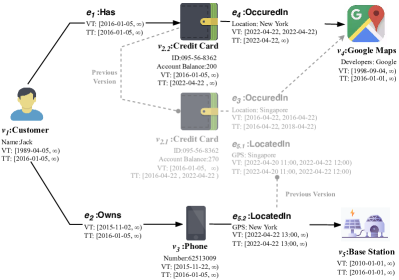
Figure 1. A credit card transaction graph with bi-temporal graph data model

2.2. Temporal Query Language

We introduce our temporal syntax by extending the regular Cypher syntax, which is combined with extensions adapted from SQL:2011 (sql-2011, ) and Allen’s interval algebra (Allen_Relationship, ).

Valid-time queries. Valid-time queries are defined as queries on valid-time graphs. As compared to the regular Cypher syntax, we include valid-time predicates from Allen’s interval relationships (Allen_Relationship, ). A valid-time query can add valid-time predicates, like OVERLAPS and CONTAINS, as the period predicates, which work together with other regular predicates in the WHERE conditions.

Transaction-time queries. Transaction-time queries are defined as queries over transaction graphs. As compared to the regular Cypher syntax, it is extended in terms of the transaction time: (1) $TT$ SNAPSHOT $t$, restricts graph objects that are readable at $t$, (2) $TT$ BETWEEN $t_{1}$ AND $t_{2}$, restricts graph objects that are readable from $t_{1}$ to $t_{2}$. We refer to the former as time-point queries and the latter as time-slice queries.

Example 2. Consider the question “What was Jack’s credit card balance on ‘2022-04-22’ recorded in database on ‘2022-04-23”’, it is expressed as follows, where the involve valid time is underlined and the transaction time is dot underlined. In particular, the valid time qualifier involved is equivalent to “DATE ‘2022-04-22” ¡ $n.VT.st$ $\leq$ DATE ‘2022-04-22 and DATE ‘2022-04-22” ¡ $r.VT.st$ $\leq$ DATE ‘2022-04-22 and DATE ‘2022-04-22” ¡ $m.VT.st$ $\leq$ DATE ‘2022-04-22”, which works together with $n.$Name=‘Jack’ in the WHERE condition.

$$\begin{array}[]{l}\text{ MATCH (n:Customer)-[r]->(m:Credit Card)}\\ \text{ WHERE n.Name=`Jack' }\\ \text{ \text@underline{VT CONTAINS DATE `2022-04-22'} }\\ \text{ \dotuline{TT SNAPSHOT DATE `2022-04-23'}}\\ \text{ RETURN m.Account Balance}\\ \end{array}$$

2.3. Temporal Constraints

Further, we define several constraints of a temporal graph, to ensure the consistency of the graph at each point in time.

For valid-time graph data model: (1) At every point in time, vertices and edges are unique by the combination of $gid$ and $VT$. (2) For each edge, there must exist two source and target vertices whose valid time contains the edge’s valid time. For transaction-time graph data model: (1) Constraints are the same as the valid-time data model, but can only be added to the current graph objects. (2) Users are not allowed to assign/change the value of transaction time, which can only be assigned/updated by the graph database system. (3) Users are not allowed to change the historical graph objects. For bi-temporal graph data model, the constraints are the combination of the valid-time graph data model and the transaction-time graph data model.

3. System overview

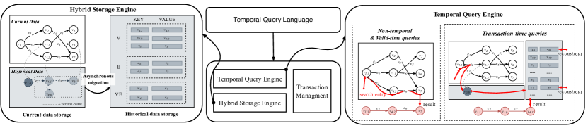
Figure 2. System overview of TGDB

We show the overview of TGDB in Figure  2. TGDB mainly extends two major components of an existing graph database to support temporal features: (1) storage engine, and (2) query engine. We next describe each of them in details.

3.1. Hybrid Storage Engine

TGDB provides a hybrid storage engine to separately store current graphs and historical graphs. We also provide a late data migration strategy to transfer data from current graphs to historical graphs asynchronously. We introduce our design from the following three aspects.

(1) Why do we use hybrid storage engine? The hybrid storage engine includes 1) current data storage engine and 2) historical data storage engine. We use the storage engine of the original graph database as current data storage engine, to store the most recent data. In addition, we attach a historical data storage engine to keep historical graphs. This design keeps a separate ‘current’ database for the most recent data. The historical data is stored in other storage engine, thus it does not affect the performance of the ‘current’ database.

(2) How to organize historical graph data? It is observed that current graph database systems mostly focus on OLTP-like CRUD operations (create, update, read, delete) for vertices and edges as well as on queries only on small portions of a graph (graph_CRUD, ). Thus it is vital to support fine-grained time management which can record the evolution of temporal graphs by only maintaining the related changed graph objects. To achieve this, instead of maintaining the versions of historical graph itself, TGDB organizes the historical graph as historical versions of graph objects. Furthermore, we only keep the data changes of every historical graph object compared to its previous version to reduce memory, from the observation that updates of graph objects are typically limited to few attribute values. Based on the considerations abouve, we use KV store as the back-end storage engine, which is suitable to store irregular data changes.

(3) When to transfer data from current to historical storage? TGDB provides a late migration strategy to transfer data from current data storage engine to historical data storage engine asynchronously. The migration is invoked periodically when the database system starts to reclaim the storage occupied by graph objects that are deleted or obsoleted, i.e, do the garbage collection. Such a late storage reclaim is common in many database systems in order to improve the efficiency of storage space and query performance.

3.2. Query Engine

The query engine executes query plans on the storage engine. Based on the design of our hybrid storage engine, we divide our queries into two categories. One is the current data queries including non-temporal queries and valid-time queries. Recall that the valid-time queries can be considered as non-temporal queries with time conditions, as described in Section 2.3. Thus they can be considered as non-temporal counterparts. This kind of query depends only on the current data storage and follows the optimization and query processing of the original database processing paradigm. The other category is transaction-time queries which involve current data storage and historical data storage. For such queries, we provide built-in operators for the execution. Once the executor recognizes transaction-time qualifiers, it invokes our extended operator execution. We provide built-in temporal support to basic operators, such as vertex scan and expanding. The overall idea of the operators is that we retrieve current and historical data on demand. Our implementation does not need to restore a full graph at a specific time point. Instead, we only reconstruct the portion of the graph of our interest. Our fine-grained access design satisfies small-scale lookup under OLTP system.

Since we get data from current data storage and historical data storage separately, we need to use transaction management to guarantee the consistency of data between two storage engines. TGDB relies on Multi-version Concurrency Control (MVCC) to support this feature. Specifically, in order to get the current data, we simply get data from the current data storage using the origin database system’s transaction mechanism. The historical data, however, need to be careful to catch. Due to the late migration strategy, not all of the historical data is in the historical storage. There will be a portion of historical data scattered on the current storage because it has not yet been migrated to the historical data storage. For those historical data on the current data storage, we use MVCC-based visibility to check whether the version is visible for a given time query. And for historical data that has been migrated to the historical data storage, we get the data of interest by simply comparing the transaction time explicitly maintained in historical storage with the user’s given time.

4. Scalable Hybrid Data Storage

TGDB uses a hybrid data storage engine to separately store current data and historical data with a late data migration strategy, as shown in Figure  LABEL:storage_overview. We first introduce how to organize the graph data in the current and historical data storage engine and then discuss the details of the late data migration strategy.

4.1. Current Data Storage

TGDB is extended on the native graph databases which employ Multi-Version Concurrency Control (MVCC) to support ACID transactions.

MVCC-based graph database. TGDB follows the MVCC system described in  (MVCC, ). Specifically, when a transaction modifies a graph object, then besides modifying the graph object in place, it also creates a delta object which described how to undo the changes of the transaction. All version deltas of a same transaction are clustered in a same undo buffer and will be together physically removed from undo buffers when the transaction is committed and no longer active. Such a mechanism maintains multiple versions for the same entity in a “newest-to-oldest” chain. Thus it is suitable for our graph data model since we can target the latest version of a graph object as the current data and old versions as historical data. It is worth mentioning that our implementation can also apply to many MVCC-based graph databases, such as commercial databases like Memgraph (Memgraph, ), ArangoDB (ArangoDB, ), OrientDB (OrientDB, ), and Dgraph (Dgraph, ), and some high-performance databases, such as G-Tran (2021G, ), Waver (Weaver, ).

Delta organization. Based on the above foundation, we target the deltas of committed transactions as historical data of graphs. We now go into great detail about how to design historical graphs with deltas. TGDB supports the evolution of graphs with both property changes and structural changes. For any vertex or edge property change, we replace in-place and generate a backward delta between the updated and the replaced version. For any deletion of a vertex or an edge, in addition to treating it as a property-clearing update, we also need to take into account structural changes. In particular, for an edge deletion, we generate a delta for the edge reflecting an attribute clear update as well as a delta for connected vertices (the edge’s incoming and outgoing vertex) including the unique identities of their previous linked edges. For a vertex deletion, we decompose it as deleting linked edges and clearing vertex attributes.

Assigning transaction-time. We now discuss how to assign transaction-time to each object in TGDB. TGDB slightly modifies the logic of transaction processing to maintain the transaction-time interval. Specifically, when a graph object $o$ is firstly created/inserted into the graph database by a transaction $T_{1}$, we assign the commit time of $T_{1}$ to $o$’s $TT.st$. When another coming transaction $T_{2}$ modifies the graph object $o$, it may generate a newly version delta $d$ (perhaps two more deltas) and we copy $o$’s $TT.st$ to $d$’s $TT.st$. Upon committing the transaction $T_{2}$, the $TT.ed$ of the delta $d$ is timestamped with the commit time of $T_{2}$. Meanwhile, the $TT.st$ of the new version of graph object $o$ is re-timestamped with the commit time of $T_{2}$. To achieve the above time allocation, we add a transaction-time field for each edge, vertex, and delta. In particular, for vertices, we additionally keep another transaction-time field for the latest graph structural changes. It helps to assign the transaction-time to the delta representing the structural change. To do so, TGDB picks the actual transaction time through transaction management while a lot of other temporal graph databases simply take the transaction time from the application level, which takes either the transaction start time or the operation time that inserts/updates/deletes the graph object. We argue this simple set can lead to an incorrect result based on the snapshot isolation theorem.

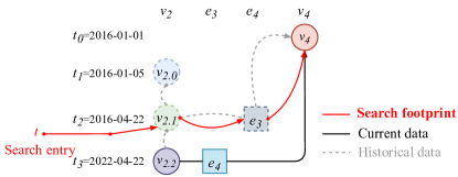
Figure 4. Search footprint

Example 3. The left part of Figure 4 shows how the graph in Figure 2 is organized in the current storage engine. Recall that TGDB translates valid-time queries into equivalent non-temporal queries, where valid-time can be simply targeted as attribute of a graph object. Thus we mainly focus on the transaction time. In general, attribute updates of vertices are indicated by blue boxes, attribute updates of edges are indicated by red boxes, and structural changes related to vertices and edges are indicated by green boxes. We can observe that in the transaction $T_{i}$, the edge $e_{4}$ was deleted from the graph database and thus generated one edge delta and two structural deltas. And another transaction $T_{i+1}$ modified the attribute balance of $v_{2}$ from 270 to 200 and generated a vertex delta. Note that we only maintain the difference compared to the new version of $v_{2}$.

4.2. Historical Data Storage

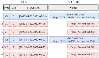
Figure 3. Placing anchor data in delta data

As discussed before, we migrate historical deltas from the current data storage to the historical data storage in the garbage collection stage. For brevity, we use unreclaimed deltas and reclaimed deltas to denote historical data in the current data storage and historical data storage respectively. In this subsection, we show how to convert unreclaimed deltas into reclaimed deltas using the key-value format to store in the KV storage.

KV format. In summary, we set the key to the combination of the prefix $Type$, the graph identifier $Gid$ and $TT$ of the delta. Here, the $Type$ contains three kinds of prefixes (1) ‘V’ for vertices, (2) ‘E’ for edges, and (3) ‘VE’ for graph topology. The $gid$ is a unique identifier of each vertex or edge. It is common in native graph databases that the system assigns a unique identifier to each vertex or edge. As for $TT$, it contains the $TT.st$ and $TT.ed$ of the delta. Obviously, the key under the above design is unique throughout the whole temporal graph. Based on such design, we transform an unreclaimed delta to a key-value format. Specifically, for a committed transaction, we collect all deltas from its undo buffer and recursively transfer each delta into the key-value pair. For the deltas linked to a same object, we will merge those deltas in one key-value pair to reduce memory. It is worth mentioning that, in the KV store, data with the same prefix is physically clustered together and different versions of the same entity are automatically sorted. For illustration purposes, the right part of Figure 4 shows how the unreclaimed deltas in the left part is organized in the KV store. Each color box represents a reclaimed delta in the KV store and matches the delta with the same color on the left. We can observe the deltas created by the transaction $T_{0}$ are of a same object and thus we merge those deltas in one key-value pair according to the order of links.

Anchor data. Maintaining only data changes reduces the overhead of storage. However, retrieval of a reclaimed graph object with a deep history incurs an expensive reconstruction cost by assembling the latest graph objects with all data changes of previous versions. To avoid this problem, we place anchor data representing complete graph objects at intervals in the delta data to shorten recovery chains and thus speed up the reconstruction. When we get a certain number of deltas of a graph object, we insert anchor data, which maintains all information about the graph object. In this way, retrieval of a certain reclaimed graph object $o_{1}$ invokes a seek of its most recent anchor data $o_{2}$, and reconstructs $o_{1}$ by assembling $o_{2}$ with all delta data from $o_{2}$ to $o_{1}$. Thus we reduce the length of the recover chain of the reconstruction. To distinguish anchor data from delta data in KV storage, we concatenate a one-bit character suffix to the type of the key, where ‘A’ is the anchor data and ‘D’ is the delta data.

Example 4. Take vertex deltas as an example, shown in Figure 5, the blue boxes are the anchor data while the red boxes are the delta data. It shows multiple versions of the graph vertex $v_{2}$. The order of deltas is organized from newest to oldest in the KV store. If we want to restore the information of the 6th delta data, we just need to restore by assembling 4th anchor with 5th and 6th delta data.

4.3. Data Migration

1 Function Migrate($CT$):

       Input: $CT$, committed transactions no longer active;

2       $undos\leftarrow\emptyset$; //unreclaimed deltas;

3       $kvs\leftarrow\emptyset$; //reclaimed deltas;

4       $undos\leftarrow undos\cup$ getUndos($CT$);

5       foreach $undo\in undos$ do

6             $kv$=encode2KV($undo$);

7             $kvs\leftarrow kv$

8      KV_store::putMultiples($kvs$);

9      

End Function

Algorithm 1 Data migration

We now discuss the details of migrating unreclaimed deltas from the current data storage engine to the historical data storage engine. In MVCC-based databases, a historical version will not be physically removed immediately, but will first be maintained in the undo buffer. Those historical versions will be physically removed only when the garbage collection triggers starts to reclaim those expired/aborted versions. This garbage collection runs periodically and reclaims versions related to committed transactions that are currently no longer active. To keep historical data, TGDB modifies the logic of the garbage collection. TGDB copies historical data from the undo buffer to the historical data storage engine before the historical data is cleaned. This late migration strategy asynchronously migrates historical data in batches and is lightweight to the original databases.

Algorithm 1 shows the details of migrating unreclaimed deltas into the historical storage. We use $undos$ to maintain the unreclaimed deltas to be migrated (line 2) and $kvs$ to store historical data in $undos$ with key-value format (line 3). We first copy all deltas from currently committed transactions (line 4). We then iteratively encode these deltas into a key-value pair $kv$, and collect all results in $kvs$ (line 5-7). Finally, we store the encoded $kvs$ in the KV store in batches (line 8).

5. Temporal Query Engine

As mentioned before, TGDB divides the queries into two categories. And only the transaction time queries are related to historical data, which we need to design carefully. To support such queries, we provide built-in operators for execution. Since the implementation of each graph database is different, we introduce our extended execution on a specific graph database. In this paper, TGDB chooses Memgraph as an original graph database to extend. Memgraph is an open-source MVCC-based commercial native graph database. The logic of its query processing is vertex-centric, which is the most basic and commonly used in graph databases. That is, to answer a query, it first scans the relevant vertices, then expands its linked edges to fetch associated vertices.

In TGDB, we extend those two basic and vital operations “scan” and “expand” to support transaction-time queries. The overall idea of our implementation is to get the current data and the historical data of interest, then integrate and return the results. For illustration purposes, we give an example to show how a transaction-time query works in Example 5.

Example 5. Figure 6 shows the search footprint of the transaction-time query of Example 3 on the graph of Example 2. Here, $v_{2}$ is the vertex we are interested and want start to scan. As we want to search graph objects at a specific time $t$, we first fetch $v_{2.1}$ satisfying the required time point. $v_{2.1}$ may be reconstructed from an unreclaimed delta or a reclaimed delta. Based on $v_{2.1}$, we next get its related edge $e_{3}$ and finally expands vertex $v_{4}$ from $e_{3}$. We integrate the historical data $v_{2.1}$, $e_{4}$ and current data $v_{4}$ and return the result.

5.1. Scan Operator

We first introduce how to fetch vertices using the scan operator. Since we store data in the current data storage and historical data storage separately, to answer a transaction-time query, we need to carefully design the operator to guarantee the consistency of these two storage engines. Recall that historical data may be unreclaimed deltas in the current data storage or reclaimed deltas in the historical data storage, due to the late migration strategy. We divide the data catching into 1) current data and unreclaimed deltas of historical data in the current data storage engine and 2) reclaimed deltas of historical data in the historical data storage engine.

1

2 Function VertexRead($C$):

       Input: $C$, temporal condition;

       Output: $\Sigma$, the result set;

3       $v\longleftarrow$ the graph vertex which we start to scan;

4       while $v$ do

5             $flag\longleftarrow$true ;

6             // get from current data storage;

7             foreach $delta\in(v\cup v.deltas)\wedge flag$  do

8                   if ! SnapshotCheck($delta$) then  continue;

9                   TemporalCheck($delta$, $C$, $\Sigma$, $flag$ );

10                  

11            //get from historical data storage;

12             if $flag$ then  FetchFromKV($v,C,\Sigma,V,flag$);

13             $v\longleftarrow v$.next();

14            

15      

16End Function

17 Function FetchFromKV($o,C,\Sigma,type,flag$):

18       $kv_{a}\longleftarrow$ $o$’s oldest version from current storage;

19       $kv_{a}\longleftarrow$ $kv_{a}/$ KV_store::seeknext($o.Gid,C$,type);

20       $kv_{d}\longleftarrow$ KV_store::seeknext($C,kv_{a}.key$,type);

21       while $kv_{d}\wedge flag$ do

22             $kv_{a}\leftarrow$ combine $(kv_{a},kv_{d})$;

23             TemporalCheck($kv_{d}$, $C$, $\Sigma$, $flag$ );

24             $kv_{d}\leftarrow kv_{d}.\texttt{next}()$

25      

26      

27

28 Function TemporalCheck ($rec,C,\Sigma,flag$):

29       if $rec.TT.st\leq{C}.t_{2}\wedge rec.TT.ed>{C}.t_{1}$ then

30             $\Sigma$ $\leftarrow$ $\Sigma$ $\cup\texttt{Reconstruct}(rec)$;

31             if $C.type=as\_of$ then $flag\longleftarrow$false;

32            

33      

34

Algorithm 2 Retrieving vertices

For the data in the current data storage engine, we catch data according to the principle of MVCC. That is, select queries always locate the latest version of the vertex, and follow its version chain recursively to find a proper version that is visible to the given query based on the snapshot isolation mechanism. To answer whether the version satisfies the given transaction-time, we additionally need check whether it satisfies the time constraint based on the following equation. Here, $C$ is a temporal condition in a transaction-time query. $C$ maintains two interval time $t_{1}$, $t_{2}$. Specially, $t_{1}=t_{2}$ for a time-point query.

(1) $$o.TT.st\leq{C}.t_{2}\wedge o.TT.ed>{C}.t_{1}$$

For the data in the historical data storage engine, it is straightforward that we get the data of interest by simply comparing the transaction time explicitly maintained in historical storage with the given time constraint of the transaction-time query. To restore a reclaimed version to a complete graph vertex, we invoke a seek of the most recent anchor delta $o_{1}$, and assemble $o_{2}$ with all data changes of versions from $o_{1}$ to $o_{2}$. Thanks to the special design of historical storage, queries with transaction-time conditions can be processed efficiently.

Algorithm 2 shows how to fetch vertices of interest from the hybrid storage engine. We start to scan from $v$, which is either the first vertex of the whole graph or the vertex pointed by the index (line 2). We first catch data from current data storage (line 6-9). We check whether $v$ or its historical unreclaimed version is visible to the current transaction’s snapshot (line 7) and satisfies the given temporal constraints using the function TemporalCheck() (line 8). Next we fetch data from historical data storage (line 10) using the function FetchFromKV(). Our idea is to find its most recent anchor data $kv_{a}$, and assemble $kv_{d}$ with all delta data of previous versions from $kv_{a}$ to $kv_{d}$. In the function FetchFromKV(), we initiate the $kv_{a}$ with the oldest version of anchor data in the current data storage, since we may not be able to find an anchor data in the KV store (line 14). Then we try to seek the nearest anchor data in the KV store according to graph object’s unique identifier $Gid$ and temporal conditions $C$. If we successfully find it, we update the $kv_{a}$ (line 15). We then seek the following deltas according to $kv_{a}$ or temporal conditions $C$ (line 16) and iteratively fetch reclaimed deltas of interest (line 17-20). During the iteration, $kv_{a}$ is combined from the previous anchor data $kv_{a}$ and current delta data $kv_{d}$ (line 18). And every $kv_{a}$ that satisfies $C$ is copied into the result set (line 20).

1

2 Function ExpandVertices ($v,C$):

       Input: $v$, the graph vertex need to expand; $C$, temporal condition;

       Output: $\Sigma$, the result set;

3       //get edges;

4       $\Sigma_{e}\leftarrow$ EdgeRead($v,C$) ;

5       FetchFromKV($v,C,\Sigma_{eid},VE,true$);

6       foreach $e_{id}\in\Sigma_{eid}$ do

7             FetchFromKV($e_{id},C,\Sigma_{e},E,true$);

8            

9      //expand vertices;

10       foreach $e\in\Sigma_{e}$ do

11             if CheckIntersect($e.TT,v.TT$) then

12                   $exp\_vid\leftarrow$ get expand vertex id from $e$;

13                   $v\leftarrow$ get vertex of $exp\_vid$ in the current storge;

14                   if Find(v) then

15                         $\Sigma_{v}\leftarrow$ VertexRead($v,C$);

16                        

17                  else

18                         FetchFromKV($exp\_vid,C,\Sigma_{v},V,true$);

19                        

20                  foreach $exp\_v\in\Sigma_{v}$ do

21                         if CheckIntersect($e.TT,exp\_v.TT$) then

22                               $\Sigma\leftarrow\Sigma\cup(e,exp\_v)$

23                        

24                  

25            

26      return $\Sigma$

End Function

Algorithm 3 Expanding Vertices

5.2. Expand Operator

We now introduce how to expand vertices using the expand operator. The query engine of TGDB is vertex-centric and edges are attached to vertices. To get vertices associated with a specific vertex, we first get linked either current or historical edges, then expand vertices from the edge Information.

Algorithm 3 shows how to expand $v$’s related vertices. Our basic idea is to fetch $v$’s related edges (line 3-6) and then expand vertices from edges (line 8-18). An edge may still maintain its most recent version in current data storage or may be deleted from current data storage. Thus, we separate the above two cases. For the first case, we get edges using the function EdgeRead(), which has the same logic of the function VertexRead() defined in Algorithm 2(line 3). For the second case, we first get $v$’s related edge identifiers from KV in the “VE” segment (line 4). And then we get the edge’s specific information in the “E” segment (line 5-6).

Next, we expand vertices based on the edges which we get from the above process. For each candidate edge $e$, we should check if the transaction time of the vertex $v$ and $e$ have an intersection based on Equation 2 (Line 13). Here, $e$ is the edge we need to check and $v$ is the vertex we want to expand.

(2) $$e.TT.ed\leq v.TT.st\wedge e.TT.st\leq v.TT.ed$$

Then we get expanded vertex id from $e$ (line 10) and check whether the expended vertex is in the current storage (line 11-12). If we find it, we fetch historical versions according to the function VertexRead() defined in Algorithm 2 (line 12-13). Otherwise, we simply get from the KV store (line 14-15). Finally, we also need to check if the transaction times of the expanded vertices and edges have an intersection (line 16-18).

6. Implementation

In this section, we present the implementation of TGDB in Memgraph, which is an open-sourced in-memory MVCC-based graph database system. Note our technology can also be applicable to other MVCC-based graph database systems with a vertex-centric query logic. To enable temporal support in Memgraph, TGDB extends the parser, storage engine, and query engine of Memgraph.

Parser. TGDB extends the parser to enable recognizing temporal qualifiers. We also add a translator API in CypherMainVisitor(), where we translate valid-time operators into equivalent non-temporal operators, and keep transaction-time operators unchanged.

Storage engine. TGDB uses hybrid storage using current data storage and historical data storage. We use the original storage in Memgraph as the current data storage and use RocksDB as a historical data storage. To integrate RocksDB into Memgraph to maintain reclaimed data, we additionally start a RocksDB process when the Memgraph instance starts. Remind we use late migration strategy to transfer unreclaimed data from current storage to historical storage. Any update/delete of a graph object will not immediately be physically removed from the current stroage. In contrast, all physical removes are periodically invoked by the system function CollectGarbage(). We modify the original function CollectGarbage() by adding an API Migrate() to transfer unreclaimed data to the RocksDB, which is defined in Algorithm 1.

Query Processor. We extend the query processor to make them capable of processing transaction-time queries. TGDB extends two basic operators: the Scan operator and the Expand operator. For the Scan operator, we extend it to support catching current vertices, unreclaimed vertices, and reclaimed vertices based on Algorithm 2 when organizing transaction-time qualifiers. For the Expand operator, we extend it to support expanding vertices for a specific vertex based on Algorithm 3.

7. Evaluation

7.1. Experimental setup

Baseline Systems. We compare TGDB with two state-of-the-art solutions: (1) the model-based approach T-GQL and (2) the snapshot-based approach Clock-G. We implemented them on Memgraph and RocksDB based on their ideas. We asked the authors if they could provide the source code, but unfortunately, their project is a corporate project and cannot be made public. Therefore, we implemented them on the same platform we applied them on, which is fair for comparison.

Configurations. The experiments were conducted on a single machine equipped with 32 Intel(R) Xeon(R) Gold 5220 CPU @ 2.20GHz, 128 GB memory, running a CentOS 7.9.2009 operation system with kernel version 3.10.0-1127.19.1.el7.x86_64. We use Memgraph with the version $v2.2.0$ and RocksDB with the version $v6.14.6$.

Dataset. We conduct the experiments using the following synthetic and real datasets. (1) LDBC: The LDBC Social Network Benchmark(LDBC SNB) is a benchmark which is designed to simulate real-world interactions in social networking applications (LDBC, ). We use its data generator to create dataset and set the scaling factor to 1. We use this benchmark to test the performance impact of temporal introduction on the original system. (2) Bi-LDBC: Bi-LDBC is a self-defined synthetic dataset. It is built on the solid foundations of LDBC dataset but extends it with a series of timestamped graph operations that simulate real-life temporal social networks. Our graph operations includes updating entities or relationships that already exist in the network and adding entities or relationships that do not currently exist in the network. In this paper, we set the scale factor to 1 on original LDBC and provide datasets with different update sizes by varying $\{1M,2M,3M,4M\}$ graph operations. (3) TPC-DS: TPC-DS is a dataset of transaction data for retail companies (TPCDS, ). This dataset includes evolution in attribute values of users, stores, items, and banks, as well as changes in customer transaction behavior, among others. The dataset we use contains data evolution from January 2000 to December 2005. We take the graph of the earliest time state of the dataset as the original graph and convert the subsequent changes into a series of timestamped graph operations. (4) E-commerce: The E-commerce dataset is a real dataset, which has been collected from a real-world ecommerce website by RetailRocket company. It is available on Kaggle (Kaggle, ) about customers’ activity on the website (views, add to cart and transactions), ranging from May 10th 2015 to September 18th 2015. Similar to the TPC-DS dataset, we transformed the data into a series of timestamped graph updates. We present some of the characteristics of datasets in Table 1 where $|V|$ refers to the total number of vertices of original graph, $|E|$ refers to the total number of edges of original graph, and Operations refers to the total number of graph operations.

Table 1. Characteristics of datasets

Dataset	$|V|$	$|E|$	Operations
LDBC	3,181,724	17,256,038	0
Bi-LDBC	3,181,724	17,256,038	1M, 2M, 3M, 4M
TPC-DS	102,546	49,559	11M
E-commerce	469,809	513,257	7M

7.2. Performance Comparison

We compare the result of our method TGDB with the model-based method T-GQL and the snapshot-based method Clock-G on Bi-LDBC dataset. We compare the performance among different methods through computing the storage consumption and query execution time. For Clock-G, we set the system parameters $N$ to 250k and $M$ to 1, which means we create a snapshot every 250k graph operations.

Workloads. Our queries include five IS queries defined in LDBC benchmark: IS1, IS3, IS4, IS5, IS7. And we additionally add time conditions into them for temporal queries. It should be highlighted that time instants used in queries are uniformly chosen within the time span of the datasets in order to avoid a biased distribution that favors only time instants closer to “snapshots”. We do not evaluate IS2 and IS6 queries for the consideration that they involve variable queries, while Memgraph cannot assign specific query conditions to variables and thus T-GQL implemented in Memgraph cannot solve such queries.

Space Overhead. We first study the storage overhead by varying the number of graph operations, as shown in Figure  5(a). We set graph operations in $\{1M,2M,3M,4M\}$ and evaluate the storage consumptions among TGDB, T-GQL and Clock-G. As shown in Figure 5(a), the storage overhead of all methods increases as the number of graph operations grows. Overall, TGDB has a much smaller storage overhead than either of the other two methods. The storage consumption of TGDB is reduced by 3.7×, 11.3× on average compared with T-GQL, Clock-G respectively. TGDB only keeps data changes of graph objects to track the evolution of graphs, so the space consumption is much smaller. Clock-G periodically creates a snapshot representing the whole graph which causes big storage overhead. And T-GQL splits a normal node into three kinds of nodes defined in  (T-GQL, ), namely Object node, Attribute node and Value node. This complex representation is costly to make the graph take more space to store nodes and edges. Furthermore, each method has a different degree of growth in storage overhead. We can observe that the storage overhead of TGDB and T-GQL grows slowly while the storage overhead of Clock-G grows rapidly. In more detail, the storage consumption of TGDB and T-GQL remains basically the same with the growth of graph operations. Compared with 1M graph operations, the storage consumption of TGDB and T-GQL grows by 1.13 times and 1.2 times respectively with 4M graph operations, while Clock-G grows by as much as 4.6 times. This is because TGDB and T-GQL only save versions of only changing graph objects while Clock-G mains versions of the graph itself.

Query Performance. We now report the results of query performance by three aspects: (1) various types of queries, (2) different scales of graph operations, and (3) query processing with index.

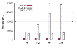
(a) Space overhead

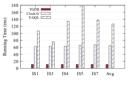
(b) Various time-point query execution time

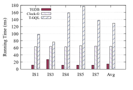
(c) Various time-slice query execution time

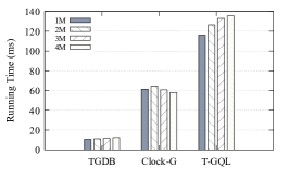
(d) Varying graph operations (time-point queries)

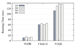
(e) Varying graph operations (time-slice queries)

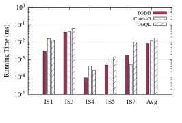
(f) Indexed query execution time

Figure 5. Performance comparison of TGDB, Clock-G, and T-GQL on Bi-LDBC

Various types of queries. We study the execution time of time-point queries and time-slice queries on IS1, IS3, IS4, IS5 and IS7, as shown in Figure 5(b) and  5(c). Overall, TGDB has the fastest query efficiency, followed by Clock-G and finally T-GQL. It can be observed that on average TGDB runs 5.7×, and 11.2× faster than Clock-G, T-GQL respectively for time-point queries and runs 4.9×, and 10.4× faster than Clock-G, T-GQL respectively for time-slice queries. Compared with Clock-G, TGDB quickly links to the historical data directly from the “current” database instead of recovering the historical graph from a snapshot before tracing the data in the log for a given point in time. In contrast with T-GQL storing the complete history in one graph, TGDB hides historical data in another storage engine thus reducing the management of irrelevant historical data. We also observe that TGDB is slightly weaker on time-slice queries than on time-point queries, which is because time-slice queries involve more historical data and we need to reconstruct a bigger set of graph objects. Furthermore, both TGDB and Clock-G perform smoothly for different types of queries for the reason that they only focus on graph objects that satisfy the time condition in the historical data. On the contrary, T-GQL behaves differently and has worse performance on IS4, IS5, and IS7 queries compared with IS1 and IS3 queries. T-GQL maintains the complete history in one graph and IS4, IS5, and IS7 queries are involved with the large-scale message entities. Those queries need more time to seek the node satisfying the condition, however, the complex design of T-GQL’s temporal graph model makes it worse.

Different scales of graph operations. We next report the execution time of time-point queries and time-slice queries by varying the graph operations, as shown in Figure 5(d) and  5(e). We can see that TGDB consistently performs better than the other two method by varying the graph operations. What is more, both TGDB and Clock-G bear little impact by the size of graph operations. Their query time remains essentially the same as the number of graph operations grows. To avoid reconstructing historical data from deep history, TGDB uses anchor data and Clock-G uses snapshots to solve this problem. In contrast, the query time of T-GQL grows with the graph operations. That’s because, in T-GQL, the size of the graph grows as time goes by and thus results in worse query performance since it’s unavoidable to traverse a larger whole graph to query just a small portion.

Query processing with index. We also evaluate the query performance with index, as shown in Figure 5(f). In this experiment, we study time-point queries on the dataset with 2M graph operations. Although TGDB has better performance on average compared with the other two methods, the performance improvement is not that prominent. TGDB runs 1.15×, and 1.83× faster than Clock-G, T-GQL respectively. It should be noted that T-GQL can not be able to create an index on a small portion of graphs since their model only includes three types of nodes. For an index query, we have to create the index on all graph objects, attributes, and attribute values in the graph, which is clearly unreasonable. Most model-based methods suffer from this problem as they support temporal features only at the application level. T-GQL performs well with such a configuration since they index on all entities of the graph, thus reducing search space. As for Clock-G, with the help of the index, it can efficiently reconstruct graph objects from snapshots without checking all graph objects in the snapshot.

7.3. Micro Evaluation

In this section, we study our system TGDB from (1) variation of interval threshold for anchor data, (2) the performance compared to the original system without temporal support and (3) the performance on the real temporal graphs.

Variation of interval threshold for anchor data. We first study the storage overhead and query execution time with different configurations by tuning the system parameters. The system parameter in TGDB is the amount of delta data between every two anchor data. We denote this parameter as $u$ and study the trade off between the storage overhead and temporal query execution time using the TPC-DS dataset, where we observe that the customer information varies a lot and thus enables us to find the golden state. We set $u$ from 1 to 1000 and query for the customer’s information at a randomly given point in time. As shown in Figure 6(a), we can observe that as the interval threshold increases, the consumptions of the storage decreases. As we use anchor data as indexes of the queries, the storage consumption increases as the interval decreases. The storage consumption decreases 1.9 times from 1 to 1000 and it has been decreasing slowly from 10 to 1000. This is because most of the single node attributes in the dataset do not change more than 100 in frequency. As for the query performance, we observe that the less $u$ takes, the shorter running time consumes. The running time of the interval threshold 1 is 2.23× faster than the running time of the interval threshold 100, which confirms that the anchor data shortens the length of the recovery version chains thus speeds up the query execution time. To balance memory consumption and query performance, we think that the appropriate parameters should be set according to the frequency of data changes. In this dataset, we suggest that the parameter $u=10$ should be set.

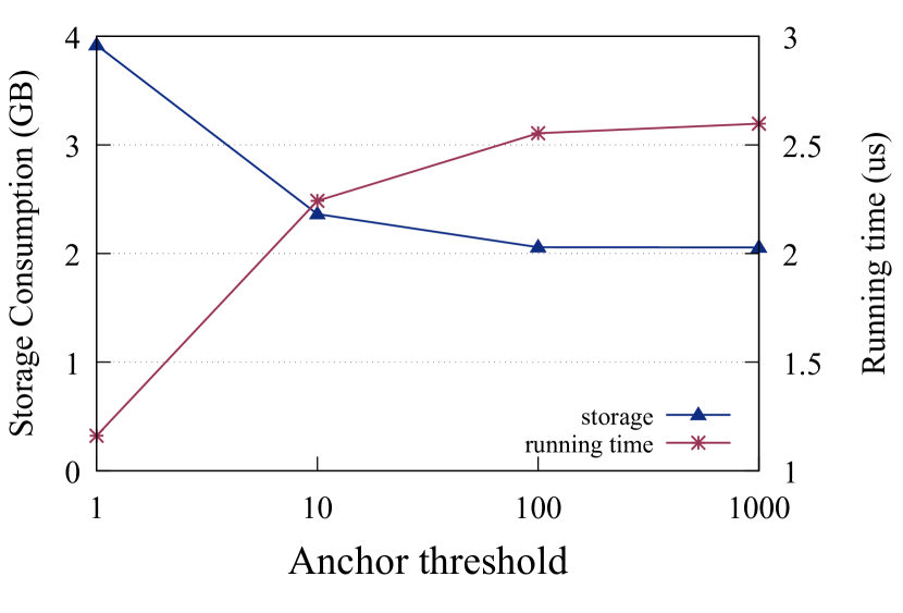
(a) TPCDS: interval threshold of anchor data

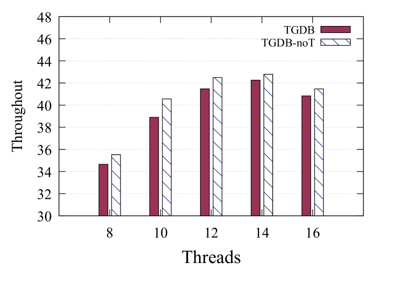
(b) LDBC: transaction throughput

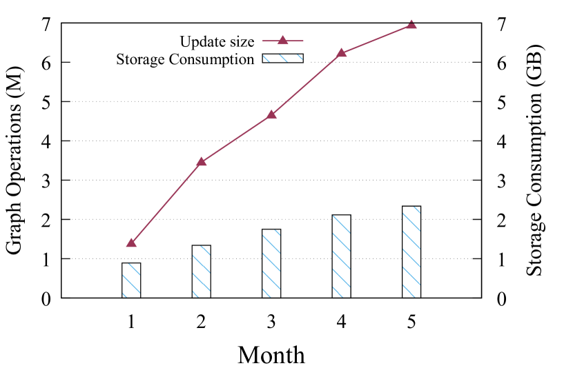
(c) E-commerce: storage overhead

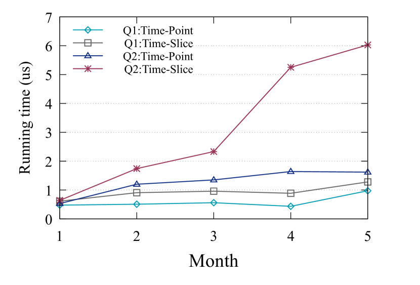
(d) E-commerce: query execution time

Figure 6. Micro Evalution.

Comparison with the original native system. We study the effect by introducing temporal support to the original graph database system on LDBC benchmark. In this experiment, we use TGDB-noT and TGDB to denote TGDB without and with temporal support, respectively. We compare the performance between TGDB-noT and TGDB in terms of transaction throughput. Figure  6(b) shows the transaction throughput of TGDB and TGDB-noT by varying the numbers of threads. It can be observed that our system’s performance is close to the origin system. By introducing temporal features, our transaction throughput is reduced by only 1.2%. This confirms that our system is less intrusive to the original system, showing that TGDB’s temporal implementation is lightweight. As repeatedly discussed before, TGDB separates “current” database and asynchronously transfers the historical data in batch only during the garbage collection invoked by the system. Such designs have minimal impact on the original system.

Evaluation on the real dataset. We evaluate TGDB on real-world dataset E-commerce from the space overhead and query execution time. E-commerce contains 5 months of variation, including modifying the item, adding the edges between users and items, etc. We constructed datasets containing 1-month, 2-month, 3-month, 4-month, and 5-month data variation respectively. The experimental result is reported in Figure  6(c) and  6(d). We use two kinds of queries, including Q1 for retrieving vertices with pure keys and Q2 for retrieving neighboring vertices/edges of a specific vertex, i.e pattern matching queries. And we randomly selected the keys of the vertices and the time periods of the queries. Figure  6(c) shows the change in the size of graph operations and storage consumption as the time span grows. It can be observed that the storage consumption grows as the size of graph operations grows. However, the storage consumption grows more slowly than the size of graph operations. It reaffirms that the storage engine of TGDB is scalable. Figure  6(d) shows the query performance of time-point queries and time-slice queries with Q1 and Q2. We can observe that the query execution time consumes longer as the time span increases.The query time for vertices is overall less than that of pattern matching. Since pattern matching queries involve more vertices and edges. And time-point queries take longer running time than time-slice queries. It is because a time-slice query returns a set of historical data for an entity or a relationship while a time-point query returns a specific historical version for an entity or a relationship.

8. Related Work

Temporal data management involves all methods and techniques to model, query and store temporal data (Temporal_Data_Management, ). There is a vast literature on this topic since the 80’s focusing on relational database management systems (RDBMS) (RDBMS1, ; RDBMS2, ; RDBMS3, ; RDBMS4, ; RDBMS5, ; RDBMS6, ). By contrast, it is not extensively studied in the context of graph management systems. The support for temporal features in graph data managements is in a patently less developed state as for their relational counterparts. To do so, we analyze existing works involving aspects of the management of temporal graph data through two primary approaches: the add-on method and the snapshot-based method.

Model-based methods. Model-based methods store and query temporal graphs by exploiting a graph database with temporal metadata. They model historical data as extra nodes and edges in one graph, which is done at the application level. Cattuto et al. (Frame, ) builds upon Neo4j and proposes a temporal model where the temporal data is represented as frames with a frame being defined as the finest unit of temporal aggregation. Campos et al. (T-GQL, ) base their research on Neo4j and addresses the problem of modeling, storing and querying temporal property graphs, allowing keeping the history of a graph database. They additionally define the Attribute and Value nodes to represent the property of a graph object and the value of the property respectively, in order to represent the evolution of graph objects’ lower level: attribute and attribute value. Other works exploit the graph database by representing the temporal dimension as an interval attribute to graph objects (liu2017keyword, ; Timebased2, ; Timebased3, ; Timebased4, ; durand2017backlogs, ). They focus on the solution of science problems like keyword searching on graph database and tracking diseases progression. Model-based methods have a strength in that they can be done on top of almost any kind of property graph model and it does not require changes to the graph database implementation. They can offer a sub-optimal way to support both transaction time and valid time. However, they rely on the complicated application logic, which is unaware of transaction commit time within the systems’ internal. Thus the transaction time is not the true commit transaction time but rather the time of the operation modifies the object. We argue this could potentially cause an incorrect result based on the snapshot isolation theorem (snapshot_isolation_theorem1, ). What is more, storing the complete history in one graph causes ever-increasing graph size and thus affects the query performance since traversing a larger graph is required. While our system is a built-in implement providing native transaction time support and we store the current data and historical data separately to speed up the query performance.

Snapshot-based methods. Snapshot-based methods consider a temporal graph as a sequence of graph snapshots, where each snapshot depicts the state of the historical graph at a past time point. Available works in this field focus on the storage and query engine to deal with the outgrowing size of data while being able to query efficiently. Copy and Log are two extreme approaches in this category. Copy approach materializes each snapshot and can be fast for queries. Chronos (Chronos, ), ChronoGraph (ChronoGraph, ) and ImmortalGraph (ImmortalGraph, ) are storage and execution engines maintaining a linear series of snapshots to keep the history of graph databases. These works provide speedup methods of the traversal over a series of snapshots. While multiple snapshots are prohibitively expensive in terms of storage, many approaches use Log to keep all graph updates as a series of timestamped logs. Koloniari et al.  (Log, ) present a model that only keeps a physical copy of the current graph and stores graph deltas externally as append-only log files. LLAMA framework (LLAMA, ) stores only the deltas between snapshots explicitly and pointers to a previous snapshot for stationary portions of the graph. These works store only graph deltas, which are space-efficient but require an expensive traversal of deltas to recover the state of the data. To balance the storage cost and query cost, a hybrid method, Copy+Log, is proposed, which combines a finite set of snapshots with a list of deltas between them. Many available temporal graph storage techniques follow this idea (copy_log1, ; xiangyu2020efficient, ; copy_log3, ; clock-g, ). However, they still suffer from a prohibitively expensive storage overhead because of the materialization of snapshots, as well as sub-optimal query performance due to overheads of graph reconstructions from snapshots and deltas. In contrast, TGDB can improve performance and reduce storage overhead at the same time by only storing and reconstructing related evolving graph objects.

Other methods. Other works manage temporal graphs in other ways. Warut D. et al.  (Scalable_time_version, ) use current table and B-tree based history table to separately store temporal graphs. Each entity type has an isolated history entries to search from history table by timestamps. However, this work does not provide a transaction manager to ensure the ACID transaction feature, which is vital in database management to guarantee the consistency of data. ChronoGraph  (ChronoGraph2, ) extends the storage, which works with time–key–value tuples as opposed to plain key–value pairs in regular key-value stores. This work provides the native support of transaction time. However, it completely modifies the underlying storage and is more invasive to the native system. In contrast, our work appends an on-demand history storage and query engine to extend the native system. It is lightweight and less invasive to the native system.

9. Conclusion

Real-world graphs are often dynamic and evolve over time. Growing interests in analyzing these dynamic graphs usually require the support of temporal data, in which two dimensions of time, valid time and transaction time, are recognized. Existing graph databases and past research works either neglect the support of transactions or valid time or support them in a sub-optimal way. In this paper, we present TGDB, a lightweight yet efficient built-in temporal implementation in graph database systems. TGDB relies on MVCC to manage temporal data and has advantages with 1) fast querying capabilities over subgraphs at a past time point or range; 2) small storage overhead of historical data; 3) native support of transaction time and valid time. In this alternative approach, we propose a hybrid data storage engine to separately manage current and historical data. Inside the historical data storage, changes of each vertex or edge are indexed for fast recoveries, and anchors are placed as snapshots to avoid deep historical version traversals. Also, we propose a temporal query engine with a novel reconstruct-as-needed solution. Our approach can only store data that has ever changed, and only reconstruct the subgraph that is needed. We integrate our approach into Memgraph and conduct extensive experiments on four real and synthetic datasets. The results show TGDB performs better both on storage overhead and query performance compared to state-of-the-art methods and has almost no performance overhead by introducing the temporal features.

References

- (1) S. Tabassum, F. S. Pereira, S. Fernandes, and J. Gama, “Social network analysis: An overview,” Wiley Interdisciplinary Reviews: Data Mining and Knowledge Discovery, vol. 8, no. 5, p. e1256, 2018.
- (2) M. Massri, Z. Miklos, P. Raipin, and P. Meye, “Clock-G: A temporal graph management system with space-efficient storage technique,” in International Conference on Data Engineering (ICDE 2022), (Kuala Lumpur, Malaysia), May 2022.
- (3) A. Abdallah, M. A. Maarof, and A. Zainal, “Fraud detection system: A survey,” Journal of Network and Computer Applications, vol. 68, pp. 90–113, 2016.
- (4) K. Kulkarni and J.-E. Michels, “Temporal features in sql: 2011,” ACM Sigmod Record, vol. 41, no. 3, pp. 34–43, 2012.
- (5) M. Haeusler, T. Trojer, J. Kessler, M. Farwick, E. Nowakowski, and R. Breu, “Chronograph: A versioned tinkerpop graph database,” in Data Management Technologies and Applications - 6th International Conference, DATA 2017, Madrid, Spain, July 24-26, 2017, Revised Selected Papers (J. Filipe, J. Bernardino, and C. Quix, eds.), vol. 814 of Communications in Computer and Information Science, pp. 237–260, Springer, 2017.
- (6) “Neo4j..” https://neo4j.com.
- (7) “Arangodb..” https://www.arangodb.com.
- (8) “Orientdb..” https://orientdb.org.
- (9) P. Gupta, A. Mhedhbi, , and S. Salihoglu, “Integrating column-oriented storage and query processing techniques into graph database management systems,” CoRR, 2021.
- (10) “Memgraph..” https://memgraph.com.
- (11) A. Debrouvier, E. Parodi, M. Perazzo, V. Soliani, and A. A. Vaisman, “A model and query language for temporal graph databases,” VLDB J., vol. 30, no. 5, pp. 825–858, 2021.
- (12) Z. Liu, C. Wang, and Y. Chen, “Keyword search on temporal graphs,” IEEE Transactions on Knowledge and Data Engineering, vol. 29, no. 8, pp. 1667–1680, 2017.
- (13) L. Zheng, L. Zhou, Z. Xin, L. Li, and W. Liu, “The spatio-temporal data modeling and application based on graph database,” in 2017 4th International Conference on Information Science and Control Engineering (ICISCE), 2017.
- (14) G. C. Durand, M. Pinnecke, D. Broneske, and G. Saake, “Backlogs and interval timestamps: Building blocks for supporting temporal queries in graph databases.,” in EDBT/ICDT Workshops, Citeseer, 2017.
- (15) W. Han, Y. Miao, K. Li, M. Wu, F. Yang, L. Zhou, V. Prabhakaran, W. Chen, and E. Chen, “Chronos: a graph engine for temporal graph analysis,” in Ninth Eurosys Conference 2014, EuroSys 2014, Amsterdam, The Netherlands, April 13-16, 2014 (D. C. A. Bulterman, H. Bos, A. I. T. Rowstron, and P. Druschel, eds.), pp. 1:1–1:14, ACM, 2014.
- (16) J. Byun, S. Woo, and D. Kim, “Chronograph: Enabling temporal graph traversals for efficient information diffusion analysis over time,” IEEE Trans. Knowl. Data Eng., vol. 32, no. 3, pp. 424–437, 2020.
- (17) Y. Miao, W. Han, K. Li, M. Wu, F. Yang, L. Zhou, V. Prabhakaran, E. Chen, and W. Chen, “Immortalgraph: A system for storage and analysis of temporal graphs,” ACM Trans. Storage, vol. 11, no. 3, pp. 14:1–14:34, 2015.
- (18) G. Koloniari, D. Souravlias, and E. Pitoura, “On graph deltas for historical queries,” CoRR, vol. abs/1302.5549, 2013.
- (19) P. Macko, V. J. Marathe, D. W. Margo, and M. I. Seltzer, “LLAMA: efficient graph analytics using large multiversioned arrays,” in 31st IEEE International Conference on Data Engineering, ICDE 2015, Seoul, South Korea, April 13-17, 2015 (J. Gehrke, W. Lehner, K. Shim, S. K. Cha, and G. M. Lohman, eds.), pp. 363–374, IEEE Computer Society, 2015.
- (20) U. Khurana and A. Deshpande, “Efficient snapshot retrieval over historical graph data,” in 2013 IEEE 29th International Conference on Data Engineering (ICDE), 2013.
- (21) L. Xiangyu, L. Yingxiao, G. Xiaolin, and Y. Zhenhua, “An efficient snapshot strategy for dynamic graph storage systems to support historical queries,” IEEE Access, vol. 8, pp. 90838–90846, 2020.
- (22) T. Neumann, T. Mühlbauer, and A. Kemper, “Fast serializable multi-version concurrency control for main-memory database systems,” in Proceedings of the 2015 ACM SIGMOD International Conference on Management of Data, pp. 677–689, 2015.
- (23) “Allen relationship - an overview — sciencedirect topics..” https://www.sciencedirect.com/topics/computer-science/allen-relationship.
- (24) M. Junghanns, A. Petermann, M. Neumann, and E. Rahm, “Management and analysis of big graph data: Current systems and open challenges,” in Handbook of Big Data Technologies (A. Y. Zomaya and S. Sakr, eds.), pp. 457–505, Springer, 2017.
- (25) T. Neumann, T. Mühlbauer, and A. Kemper, “Fast serializable multi-version concurrency control for main-memory database systems,” in Proceedings of the 2015 ACM SIGMOD International Conference on Management of Data, Melbourne, Victoria, Australia, May 31 - June 4, 2015 (T. K. Sellis, S. B. Davidson, and Z. G. Ives, eds.), pp. 677–689, ACM, 2015.
- (26) “Dgraph..” https://dgraph.io.
- (27) H. Chen, C. Li, C. Zheng, C. Huang, J. Fang, J. Cheng, and J. Zhang, “G-tran: Making distributed graph transactions fast,” 2021.
- (28) A. Dubey, G. D. Hill, R. Escriva, and E. G. Sirer, “Weaver: A high-performance, transactional graph database based on refinable timestamps,” 2015.
- (29) A. Iosup, M. Anderson, I. G. Tnase, Y. Xia, and N. Sundaram, “Ldbc graphalytics: a benchmark for large-scale graph analysis on parallel and distributed platforms,” Proceedings of the Vldb Endowment, vol. 9, no. 13, pp. 1317–1328, 2016.
- (30) “Tpc-ds..” http://www.tpc.org/tpc_documents_current_versions/pdf/tpc-ds_v2.13.0.pdf.
- (31) “Kaggle..” https://www.kaggle.com/datasets/retailrocket/ecommerce-dataset?select=item_properties_part2.csv.
- (32) M. H. Böhlen, A. Dignös, J. Gamper, and C. S. Jensen, “Temporal data management - an overview,” in Business Intelligence and Big Data - 7th European Summer School, eBISS 2017, Bruxelles, Belgium, July 2-7, 2017, Tutorial Lectures (E. Zimányi, ed.), vol. 324 of Lecture Notes in Business Information Processing, pp. 51–83, Springer, 2017.
- (33) A. Bolour, T. L. Anderson, L. J. Dekeyser, and H. K. T. Wong, “The role of time in information processing: a survey,” SIGART Newsl., vol. 80, pp. 28–46, 1982.
- (34) R. T. Snodgrass and I. Ahn, “A taxonomy of time in databases,” in Proceedings of the 1985 ACM SIGMOD International Conference on Management of Data, Austin, Texas, USA, May 28-31, 1985 (S. B. Navathe, ed.), pp. 236–246, ACM Press, 1985.
- (35) G. Özsoyoglu and R. T. Snodgrass, “Temporal and real-time databases: A survey,” IEEE Trans. Knowl. Data Eng., vol. 7, no. 4, pp. 513–532, 1995.
- (36) A. U. Tansel, J. Clifford, S. K. Gadia, S. Jajodia, A. Segev, and R. T. Snodgrass, eds., Temporal Databases: Theory, Design, and Implementation. Benjamin/Cummings, 1993.
- (37) C. J. Date, H. Darwen, and N. A. Lorentzos, Temporal data and the relational model. Elsevier, 2002.
- (38) B. Salzberg and V. J. Tsotras, “Comparison of access methods for time-evolving data,” ACM Comput. Surv., vol. 31, no. 2, pp. 158–221, 1999.
- (39) C. Cattuto, M. Quaggiotto, A. Panisson, and A. Averbuch, “Time-varying social networks in a graph database: [a neo4j use case],” in First International Workshop on Graph Data Management Experiences and Systems, 2013.
- (40) H. Memarzadeh, N. Ghadiri, and S. P. Zarmehr, “A graph database approach for temporal modeling of disease progression,” in International Conference on Computer and Knowledge Engineering.
- (41) M. Yu, “A graph-based spatiotemporal data framework for 4d natural phenomena representation and quantification-an example of dust events,” ISPRS Int. J. Geo Inf., vol. 9, no. 2, p. 127, 2020.
- (42) H. Berenson, P. A. Bernstein, J. Gray, J. Melton, E. J. O’Neil, and P. E. O’Neil, “A critique of ANSI SQL isolation levels,” in Proceedings of the 1995 ACM SIGMOD International Conference on Management of Data, San Jose, California, USA, May 22-25, 1995 (M. J. Carey and D. A. Schneider, eds.), pp. 1–10, ACM Press, 1995.
- (43) W. Han, K. Li, S. Chen, and W. Chen, “Auxo: a temporal graph management system,” Big Data Min. Anal., vol. 2, no. 1, pp. 58–71, 2019.
- (44) M. Massri, P. Raipin, and P. Meye, “Gdbalive: a temporal graph database built on top of a columnar data store,” Engineering and Technology Publishing, no. 3, 2021.
- (45) W. D. Vijitbenjaronk, J. Lee, T. Suzumura, and G. Tanase, “Scalable time-versioning support for property graph databases,” in 2017 IEEE International Conference on Big Data (IEEE BigData 2017), Boston, MA, USA, December 11-14, 2017 (J. Nie, Z. Obradovic, T. Suzumura, R. Ghosh, R. Nambiar, C. Wang, H. Zang, R. Baeza-Yates, X. Hu, J. Kepner, A. Cuzzocrea, J. Tang, and M. Toyoda, eds.), pp. 1580–1589, IEEE Computer Society, 2017.