Equations discovery of organized cloud fields: Stochastic generator and dynamical insights

Abstract

The emergence of organized multiscale patterns resulting from convection is ubiquitous, observed throughout different cloud types. The reproduction of such patterns by general circulation models remains a challenge due to the complex nature of clouds, characterized by processes interacting over a wide range of spatio-temporal scales. The new advances in data-driven modeling techniques have raised a lot of promises to discover dynamical equations from partial observations of complex systems.

This study presents such a discovery from high-resolution satellite datasets of continental cloud fields. The model is made of stochastic differential equations able to simulate with high fidelity the spatio-temporal coherence and variability of the cloud patterns such as the characteristic lifetime of individual clouds or global organizational features governed by convective inertia gravity waves. This feat is achieved through the model’s lagged effects associated with convection recirculation times, and hidden variables parameterizing the unobserved processes and variables.

I Introduction

For complex systems, most models only resolve spatio-temporal scales and processes to a certain level of accuracy due to the high computational costs associated with high-fidelity simulations on one hand, and to poor understanding of the governing subgrid or coupled processes, on the other. Such truncations of scales often limit the accuracy and reliability of the simulations of certain features. This is particularly true for general circulation models (GCMs) which are unable to resolve the details of cloud fields’ organization, due to their coarse resolution. Cloud resolving models, focusing typically on regional scales, include more detailed physics and involve finer-grid resolution schemes resulting into a much greater realism of simulated organized cloud patterns [1], at the expense though of heavy computations requiring supercomputers.

In many applications, the neglected and unresolved variables along with their interactions with the resolved ones are thus key to resolve. Parameterizations of these ingredients are often sought to provide closure models also known as reduced-order models in engineering. These models are aimed at faithfully emulating solutions of the fully resolved problem while solving only a subset of variables of interest; e.g. [2, 3, 4].

It is where closure formalisms serve as a theoretical guidance to know the mathematical ingredients required for stable and accurate approximations of the dynamics, given a truncation of the variables characterizing the full system’s state. Many such formalisms are available from turbulence theory [5, 6], quantum field theories [7], to statistical physics [8, 9] as well ideas pertaining to stochastic modeling of unresolved space-time scales in climate models [10, 11].

However, often, the master equations of a given observed phenomenon are yet to be known and several components and processes are to be imagined, with only a degree of partial success, especially for the appropriate modeling of large-scale organizational features and related small scales dynamics/processes affecting them. A range of issues and challenges need to be addressed to realize this feat.

The new advances in data-driven stochastic modeling techniques over the last decades opened up prodigious perspectives for tackling this problem. These methods have indeed shown to be skillfull for finding from partial observations of a complex system, a few dynamical equations—called data-driven closure models—that are able to simulate with reliability various complex phenomenas. These include the modeling of El-Niño-Southern Oscillation (ENSO) [12, 13, 14, 15, 16, 17], paleoclimate [18], oceanic turbulence [19, 20, 21], atmospheric dynamics [22, 23, 24], the Madden-Julian Oscillation [25, 26, 27], or the Arctic sea ice [28, 29, 30] to name a few.

A common thread is at the core of the derivation of such reliable data-driven closure models. It consists of the efficient learning of surrogate stochastic variables along with their interaction laws with the observed ones that are altogether able to emulate the missing dynamical information, central in the organization of e.g. the observed large-scale patterns. A theoretical guiding framework has emerged to achieve such features, namely the Mori-Zwanzig (MZ) formalism from statistical physics [8, 9], extended to a modern and general framework by Chorin et al. in [31, 32]; see also [33, 34, 35, 36, 37]. This framework predicts the existence of a closed form for describing the time-evolution of e.g. coarse-scale observations issued from a high-dimensional system, without having to resolve the small scales. Within this framework, the resulting closure is stochastic, made of Markovian terms that usually describe the average (slow) behavior of the observed variables augmented by (possibly nonlinear) “memory” plus “noise” terms, aimed at restoring the effects of the neglected/unobserved variables, i.e. to parameterize their feedback onto the resolved variables [34, 36].

In other words, the MZ theory ensures that a close equation for the coarse-scale variables, $\bm{x}(t)$, takes the form of the following Generalized Langevin Equation (GLE) [34, 36, 37]:

$$\dot{\bm{x}}=\bm{\mathcal{M}}(\bm{x}(t))+\int_{0}^{t}\bm{\Gamma}(t-s)\bm{\mathcal{N}}(\bm{x}(s))\,\mathrm{d}s+\bm{\eta}(t),$$ (1)

in which $\bm{\mathcal{M}}$ and $\bm{\mathcal{N}}$ are (possibly) nonlinear mappings of the state space of coarse-scale variables, $\bm{\Gamma}(t-s)$ is typically a time-lagged damping operator, and $\bm{\eta}(t)$ is interpreted as an effective random forcing uncorrelated with the time-evolution of the resolved variable, $\bm{x}(t)$, which can itself exhibit strong correlation in time though, e.g. red noise and beyond; see e.g. [38]. In the MZ jargon, the terms in $\bm{\mathcal{M}}$ are referred to as Markovian, the integral terms as non-Markovian, and the term $\bm{\eta}$ is simply referred to as noise.

Depending on the situation, not all the terms are necessarily needed in this MZ “manifesto” for closure, and different gradations of prominence between them arise in applications. The closure may for instance require either Markovian terms to be highly nonlinear without need of memory and noise terms [39, 40], either linear Markovian terms augmented by memory and noise terms involving nested temporal convolutions [17, 41, 42], delay effects [43], or a carefull blend of such elements [44, 45, 42, 46, 47, 43, 38].

In its generality, Eq. (1) provides the backbone of closure of chaotic forced systems with disparate scale interactions among their variables, and without neat scale separation as encountered for e.g. various climate processes [48]. The noise and memory terms can be however extremely complicated to calculate, especially in cases with such weak or no obvious timescale separation between the resolved and unresolved variables [49]. The approximation of these terms constitutes thus the main theme of most research on the MZ decomposition (1).

Many techniques have been proposed to address this problem in practice and can be grouped in two categories: (i) data-driven methods, and (ii) methods based on analytical insights tied to the very derivation of the MZ decomposition [37]. Data-driven methods aim at recovering the MZ memory integral and fluctuation terms based on data, by exploiting sample trajectories of the full system. Typical examples include the NARMAX (nonlinear auto-regression moving average with exogenous input) technique developed by [46, 47, 50], the rational function approximation proposed in [51], the conditional expectation techniques of [52], methods exploiting neural networks architectures to learn the memory terms [53, 54], and methods based on Markovian approximations by means of surrogate hidden variables [55, 41, 42, 51].

In this study, we adopt the Markovian approximation approach of [55, 42] which benefits from theoretical foundations [56] and allows for useful interpretations as explained below. This approach relates, in its formalism, to higher-order Taylor approximations of the memory integrand as framed in [49] and allows for rigorous error estimates [57]. In [49, 57] the memory and noise terms are approximated by solving iterative layered systems of dynamical equations in which the forcing at one level is the variable of the next one. Similarly, the approach of [55, 42] involves multilayered stochastic differential equations (SDEs)—called Multilayer Stochastic Models (MSMs)—of the form

$$\dot{\bm{x}}=G(\bm{x}(t))+\bm{r}_{0}(t),$$ (2)

$$\dot{\bm{r}}_{n-1}=\mathcal{F}_{n-1}(\bm{x}(t),\bm{r}_{n-1}(t))+\bm{r}_{n}(t),\;n=1,\cdots,N,$$

$$\mbox{with }\bm{r}_{N}(t)=\bm{Q}\dot{{\bm{W}}}_{t},$$

where the matrix $\bm{Q}$ is the square root matrix arising in the Cholesky factorization of the covariance matrix of the last level residual $\bm{r}_{N}$. The vector $\dot{{\bm{W}}}_{t}$ has its components made of mutually independent white noises.

In its original formulation [55, 14], the terms $G$ were sought to be quadratic and the $\mathcal{F}_{n-1}$ as linear matrices. More general forms of admissible $G$ and $\mathcal{F}_{n-1}$ while ensuring solutions’ stability were framed in [42, Corollary 3.2]. The usage of Eq. (LABEL:Eq_Hmodel) as a mean of approximation of the memory and noise terms of the GLE (1) was pointed in [42, Proposition 3.3] and substantiated in [56]. This is essentially obtained by bottom-up integration, from the last equation to the first one, leading to memory and nosie terms involving repeated convolutions in time.

Whatever the form of $G$ and the $\mathcal{F}_{n-1}$ retained, the philosophy behind Eq. (LABEL:Eq_Hmodel) is simple to explain. The term $\bm{r}_{0}$ in the first equation of Eq. (LABEL:Eq_Hmodel) can be viewed as the residual obtained by regressing $\dot{\bm{x}}$ onto $G(\bm{x}(t))$ (for a given class of $G$). In practice, this residual is correlated with the observed variables $\bm{x}(t)$ explaining thus the choice of the second equation conditioning the rate of change of $\bm{r}_{0}$ onto $\bm{x}(t)$. The procedure is iteratively continued until the residual becomes (ideally) uncorrelated with the observations, propitious for its approximation by white noise. The class of functions $G$ and the $\mathcal{F}_{n-1}$ are aimed to be tuned in the course of the procedure for the latter condition to hold.

The stochastic process $\bm{r}_{0}(t),\cdots,\bm{r}_{N-1}(t)$ can be then viewed as hidden variables parameterizing the neglected variables. After bottom-up integration of Eq. (LABEL:Eq_Hmodel), they take the form of integral terms depending on the past of $\bm{x}(t)$ added to stochastic convolutions approximating the memory and noise terms in Eq. (1)) [42, Proposition 3.3]. These hidden variables are thus intended at modeling the effects of the neglected/unobserved scales on the dynamics of the resolved variable $\bm{x}(t)$.

Figure 1: The quest of data-driven closure modeling. The purpose consists from high-resolution observations of (i) deriving reduced coordinates enabling (ii) an efficient learning of a data-driven closure model in order to generate in turn, at a cheap numerical cost, reliable large ensemble statistics of an observed phenomenon.

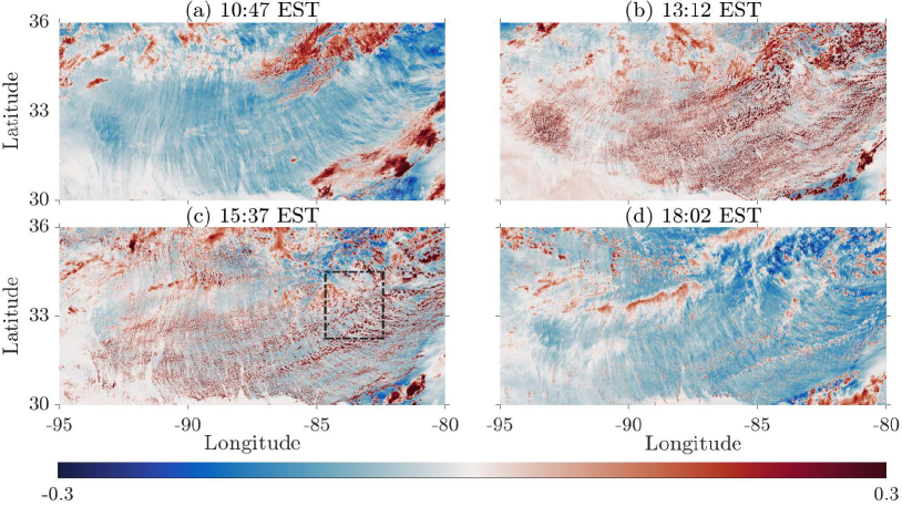
Figure 2: High-resolution (corrected) reflectance anomaly field of the diurnal cloud evolution as obtained from GOES–16 ABI’s “Red” visible band (channel 2; $0.64\,\mu m$); see Appendices A and B. Here are shown snapshots taken at 10:47 (a), 13:12 (b), 15:37 (c), and 18:02 (d) EST.

The present study adopts thus the MSM approach [42] to derive approximations of the GLE (1), in the context of cloud dynamics. The goal is to derive MSMs, from high-resolution satellite observations of clouds, that are able to provide reliable data-driven closure models at a cheap numerical cost and to investigate the dynamical insights that such models can glean; see Fig. 1. In particular, we aim by this approach at the characterization and simulation of organized patterns formed by shallow convective clouds [58, 59, 60, 61] and their underlying dynamics. To do so, we restrict ourselves to a special but common class of continental shallow convective clouds. This subset of cloud fields, defined as green-cumulus (greenCu), have strict morphological properties, narrow cloud’s size distribution and well defined organized patterns that exhibit street or grid shapes [61, 62]. GreenCu fields are known to form over forests or vegetated areas [63, 64], to share universal properties, especially in the way these clouds are organized in time and space [64] at a wide variety of climatological environments from the tropics to the mid-latitudes [64]. Yet, shallow Cu mesoscale’s organization is not properly represented in global circulation models, in spite of their role on the Earth’s radiation budget and overall climate sensitivity due to uncertainty associated with low clouds feedback [65, 66, 67, 68]. In this sense, our approach provides an alternative route to the modeling of cloud field organization from satellite observations, which, as demonstrated below, is promising in terms of its ability to extract physical insights, at a low-computational cost.

The remainder of this paper is organized as follows. We introduce our cloud dataset and describe our stochastic cloud model in Sec. II. In Section III, we provide first evidences of the ability of the stochastic cloud model to simulate clouds in the visible domain in a consistent way with the observations. To better assess the performances of our stochastic cloud model we describe in Sec. IV our approach to extract spatio-temporal coherent modes from observations as well as simulations. Our stochastic cloud model is then compared to observations in Secns. V and VI in terms of spatio-temporal variability of the simulated clouds through the analytical insights that these modes provide. We show in particular that the simulated cloud patterns reproduce with a great accuracy the characteristic lifetime of individual clouds as well as global organizational features governed by convective inertia gravity waves. We conclude in Sec. VII by discussing the implications of our results in the context of the modeling of cloud field organization.

II Multilayer Stochastic Model of Clouds

We describe in this section our MSM greenCu model. The training of our MSM’s parameters is performed with only 1 day of available high-resolution satellite data corresponding to channel 2 of the Advanced Baseline Imager on GOES-16, $0.64$ micrometers, which reflects visible solar radiation from GOES-16 [69] for a total of 8 hours collected every 5 minutes (97 2-D snapshots). Figure 2 shows a segment in the life of the cloud patterns (as revealed by reflectance anomalies) we aim to model. Our modeling takes place in the Empirical Orthogonal Function (EOF) space [70] of the reflectance anomaly field following [61]; see also Appendix A.

In the context of the GOES-16 greenCu dataset considered here, it turned out that a simple 1-layer MSM ($N=1$ in Eq. (LABEL:Eq_Hmodel)) with linear interactions ($G$ and $\mathcal{F}_{0}$ linear) is sufficient to capture faithfully the observed cloud dynamics over the region of interest, with the addition though of new ingredients in the form of explicit lagged variables into the MSM. More exactly, our MSM model of shallow convective clouds writes

$$\dot{\bm{x}} =\bm{A}_{0}\bm{x}+\sum_{k=1}^{p}\bm{A}_{k}\bm{x}(t-k\tau)+\bm{r}(t)$$ (3a)

$$\dot{\bm{r}} =\bm{B}_{0}\bm{r}+\sum_{k=1}^{q}\bm{B}_{k}\bm{r}(t-k\tau)+\bm{C}\bm{x}+\bm{Q}\dot{{\bm{W}}}_{t}.$$ (3b)

Here, the $d$-dimensional vector time series, $\bm{x}(t)$, is aiming at modeling a subset $\bm{x}_{\textrm{obs}}(t)$ of the Principal Components (PCs) extracted by EOF decomposition of the greenCu’s reflectance anomalies collected from the given dataset [61]. We emphasize that many other dynamical variables play a key role in the organization and the evolution in time of this reflectance field but are unavailable from satellite data [64]. As recalled above the inclusion of lagged effects and the auxiliary variable $\bm{r}(t)$ are aimed at accounting for the organizational effects of these hidden factors.

Furthermore, inclusion of explicit lagged effects in the formulation of Eq. (3) compared to Eq. (LABEL:Eq_Hmodel) is aimed at resolving certain characteristic timescales that are more amenable under this format than by integral terms (with decaying kernel) as typically arising in standard MSMs. For instance such terms may be advocated to originate from the recirculation time of the flow in the confined space imposed by shallow convection [71]. We refer to [71] for oscillations resulting from the delayed coupling of boundary layer instabilities by slow convective motion of the recirculation, in the case of Rayleigh-Bénard convection.

More generally, such delay terms characterize feedback mechanisms and have shown their relevance in a variety of climate applications [72, 73, 74, 75, 43], including cloud dynamics [76, 77, 78, 1]. They have been recently proposed as arising from application of the MZ formalism in the derivation of reduced equations [43], supporting thus our postulate here.

In Eq. (3), the $d$-dimensional vector $\bm{r}(t)$ which forces the main level Eq. (3a), is obtained by integration of the second level Eq. (3b), itself forced by the main-level variable $\bm{x}(t)$ and driven by a $d$-dimensional Brownian process ${\bm{W}}_{t}$. The matrices $\bm{A}_{k}$, $\bm{B}_{k}$ are $d\times d$-matrices with real entries, as well as the matrix $\bm{C}$. These entries are here estimated via two successive regressions from data which due to the shortness in time of data are learned using regularization methods; see Appendix C. First the entries for the $\bm{A}_{k}$’s are estimated by regressing, $\delta\bm{x}/\tau$ ($\delta\bm{x}=\bm{x}(t+\delta t)-\bm{x}(t)$), onto the right-hand-side (RHS) of Eq. (3a) in which $\bm{x}(t)$ is replaced by the vector $\bm{x}_{\textrm{obs}}(t)$ of observed PCs in Eq. (3a) and $\tau$ denotes the sampling time at which the data is available. After this regression, the residual $\bm{r}(t)$ is formed. In a second step, the entries of the $\bm{B}_{k}$’s and $\bm{C}$ matrices are then estimated by regressing the increments, $\delta\bm{r}/\tau$, of the first regression residual, $\bm{r}(t)$, against the RHS of Eq. (3b), while the positive definite matrix $\bm{Q}$ is obtained as the Cholesky decomposition of the covariance matrix of the residual obtained from this second regression [79, 42]; see also [12].

This noise covariance matrix, implicitly encoding across the channels the spatial coherent information at the residual level, is estimated along with other deterministic coefficients and further used to generate a spatially coherent white noise process (the $\bm{Q}\dot{{\bm{W}}}_{t}$-term) for driving the stochastically forced simulations. For the GOES-16 greenCu dataset, we selected $d=16$ corresponding to the 16 leading EOFs capturing about 60 $\%$ of the variance. The optimal choice as guided by a whitening criterion (see below) leads to $p=5$ and $q=2$, while $\tau$ corresponds here to the sampling frequency at which the data is available, i.e. $\tau=5$ min.

Note that since $p=5$ in Eq. (3), the future of $\bm{x}(t)$ is conditioned upon its previous states up to 25 min from the past. The latter timescale is consistent with a convection recirculation time in between 15 to 25 min such as observed for such shallow convective clouds [61]. In absence of the noise term, the dynamics from Eq. (3) consists of a damped oscillation which eventually settles down to a steady state while when turned on, the noise term, modeling the unobserved fast processes, triggers a rich range of spatio-temporal patterns that are analyzed below. Thus, the process $\bm{r}(t)$ that acts as a forcing in Eq. (3a) injects energy for sustaining these oscillations, while its dependence on $\bm{x}(t)$ (and past values) are key to resolve properly for triggering the right temporal variability.

As mentioned above, the rationale behind Eq. (3b) consists of observing that typically the residual $\bm{r}(t)$, obtained after learning the coefficients of Eq. (3a), is often correlated with $\bm{x}(t)$. Thus Eq. (3b) is aimed at providing an evolution law for $\bm{r}(t)$ that depends on $\bm{x}(t)$, whose ingredients are chosen with the purpose of reaching some form of “whitening” of the 2nd residual error $\bm{r}_{1}$ obtained after learning the constitutive elements of Eq. (3a); see [42]. If for the dictionary used for these elements (e.g. linear and quadratic functions), this whitening is not reached, one then either augment the dictionary of functions or further regress $\delta\bm{r}_{1}/\tau$ onto another functional form involving $\bm{x}(t)$ and $\bm{r}(t)$ (as in Eq. (LABEL:Eq_Hmodel)). We repeat the procedure then as needed until a whitening criterion of the residual is satisfied [42, Appendix A]. For theGOES-16 greenCu reflectance dataset at hand, the functional form of Eq. (3) with its 1-layer structure is sufficient to reach such a near-whitening of $\bm{r}_{1}$. In particular, this is the way the model parameters $p$ and $q$ are chosen, so that the components of the vector $\bm{r}_{1}(t)$ have negligible autocorrelation at lags equal or larger than the sampling time $\tau$, to ensure a reasonable approximation by white noise [42, Appendix A]. Note that when these model parameters and the matrices involved in Eq. (3) are learned, $\bm{r}(t)$ in Eq. (3a) depends on the past values of $\bm{x}(t)$ (after integration of Eq. (3b)) and in that sense $\bm{x}(t)$ expresses a form of Granger causality in the prediction of $\bm{r}(t)$[80].

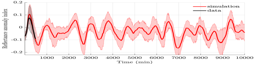
Figure 3: Time evolution of the index consisting of averaging the reflectance anomalies over an area $\mathcal{O}$ (dashed box in Fig. 2c), dominated by cloud street patterns exhibited over continental US. The grey and light-red shaded areas show the index variance over the region $\mathcal{O}$ from observations and from simulations, respectively. Note the dominant 800-min period ($\sim$ half-day) of the simulated oscillations maintaining thus the simulated MSM reflectance anomalies in the visible.

III Time-variability analysis: First results

To conduct a first assessment of the MSM cloud model’s ability to capture the variability of the observed greenCu field, we construct the system’s observable which consists of averaging the reflectance anomalies over an area $\mathcal{O}$ (dashed box in Fig. 2c) dominated by cloud street patterns. The black curve in Fig. 3 shows the evolution of this index for the time frame of available observations ($\sim 8$ hrs) used to calibrate the MSM model’s parameters in Eq. (3).

The same index as calculated from a long-term simulation of Eq. (3), shown by the red curve in Fig. 3, exhibits a prominent oscillatory period corresponding to about half of the diurnal cycle consistent with the fact that the observations are collected in the visible range from GOES-16. The MSM model does not predict thus episodes over night that would be inconsistent with the modeled variables, namely reflectance anomalies collected during daylight.

The MSM cloud model is thus able to simulate a sort of “groundhog half-day” (half as trained in the visible) with its own scenery of events taking place in the visible band, that albeit displaying repetitive features allow for variability in their statistical occurrence. As a foreshadowing of the results ahead, when used as a statistical generator of spatio-temporal shallow convective cloud patterns, the MSM cloud model allows for gaining in turn insights about the dynamics of the latter; insights that are hardly accessible from raw and short observations, otherwise.

IV Spatio-Temporal Coherent Modes

We plan now to analyze in more details the spatio-temporal variability as simulated according to Eq. (3). In particular, we are after spatially correlated structures associated with oscillations that can serve for comparison with observations. Such patterns can be extracted in many ways by applications of statistical methods such as based on principal component analysis [70] and the like [81, 82, 83]. The last two decades have seen the emergence of promising alternatives that seek for patterns with genuine dynamical features based on rigorous operator-theoretic approaches, rather than on intuitive statistical constructs. The grand purpose consists of interrogating the dynamical generator behind the time-sequential dataset under investigation. Two class of methods have attracted a lot of attention in that respect. Those based on the Koopman operator applied to Eulerian datasets [84, 85, 86, 87]; and those based on the transfer operator and its various Makovian-Ulam approximations applied typically to Lagrangian datasets [88, 89]. In [90], the data-adaptive harmonic decomposition (DAHD) was proposed as a third class of methods based on operators built from the shift semigroup’s action on cross-correlation functions. Recently, relationships with Koopman-based decomposition methods have been elucidated in [91].

In this study, we apply DAHD to extract our spatio-temporal coherent modes from either simulations or observations. Each of these modes extracted by DAHD, called DAH modes (DAHMs), is naturally associated with a Fourier frequency $\bm{\omega}_{k}$ and contains furthermore a data-adaptive phase information, ranked per $\bm{\omega}_{k}$, in their very fabric [90, Theorem V.1]. This phase information is an important feature to capture phase coherent patterns constituted of a mixture of synchronized and disorganized states as typically observed in geophysical datasets.

Given e.g. the vector $\bm{x}(t)$ solving Eq. (3) or the observed PCs from the GOES-16 dataset, the DAHMs are obtained via eigendecomposition of a grand block-Hankel matrix, $\bm{H}$, formed out of time-lagged cross-correlations between either the components of $\bm{x}(t)$ or of the PCs in the case of observations; see Appendix D. The theory of [90] shows that for a multivariate signal made of $L$ channels (here the PCs or $\bm{x}(t)$), a DAHM has a temporal dimension made per channel by time-lagged coordinates associated with the maximum time-lag $M$ used to estimate the time-lagged cross-correlations. Each DAHM’s component is made of pure sines along the temporal dimension, which are shifted one to another according to a phase relationship depending on $\bm{\omega}_{k}$; see Eq. (LABEL:Eq_DAHM) in Appendix D. It is this frequency- and channel-dependent phase information that gives the data-adaptive character of a DAHM.

The DAHMs can be grouped furthermore per frequency, $\bm{\omega_{k}}$, into $L$ pairs $(\mathbf{E}^{j},\overline{\mathbf{E}}^{j})$ whose each temporal component of $\mathbf{E}^{j}_{\ell}$ for a given channel $\ell$, is is in phase quadrature with that of the same channel in $\overline{\mathbf{E}}^{j}$; see Appendix D. Then, the presence or not of spatially correlated structures at the frequency $\bm{\omega_{k}}$, is simply revealed by looking at the spatio-temporal mode, $\mathcal{D}_{j}$, periodic in time of period $\bm{\omega_{k}}^{-1}$, and given in the physical domain by

$$\mathcal{D}_{\ell}(t,x,y)=\sum_{\ell}\textrm{EOF}_{\ell}(x,y)\Big{(}\mathbf{E}^{j}_{\ell}(t)+i\overline{\mathbf{E}}^{j}_{\ell}(t)\Big{)},$$ (4)

(with $i^{2}=-1$) in which $\textrm{EOF}_{\ell}$ denotes the $\ell$-th EOF mode, while the time $t$ runs through the lags used to compute the temporal correlations to form the block-Hankel matrix $\bm{H}$. The presence of the factor, $\mathbf{E}^{j}_{\ell}(t)+i\overline{\mathbf{E}}^{j}_{\ell}(t)$, in the sum (4) is meant to extract the spatially coherent information across the EOFs, at the given frequency.

To go back to the original physical time (and not the time-lagged coordinates), one builds to each such a mode a reconstructed component (RC) through a simple projection of the dataset onto this mode, providing in turn the contribution of this mode as expressed in the original spatio-temporal dataset, allowing in particular for time-modulation; see [20]. The DAHMs allow thus, through their RCs, for an alternative representation/decomposition of the data in terms of oscillatory patterns whose evolution in time is narrowband in frequency around $\bm{\omega}_{k}$, the frequency of the corresponding DAHM pair.

V Multivariate Power Spectral Analysis

Since each DAHM is naturally associated with a Fourier frequency $\bm{\omega}_{k}$, one can form a multidimensional power spectrum by simply sorting out the corresponding eigenvalues $\lambda_{j}$ of $\bm{H}$ against the frequencies $\bm{\omega}_{k}$. The resulting DAHD power spectrum informs us on the energy content of the multivariate signal at each frequency $\bm{\omega}_{k}$ [90, Remark V.1-(ii)] and coincides with the standard power spectrum for univariate signals [90, Theorem IV.1]. The DAHD power spectrum allows thus for extending standard power spectral interpretations holding for univariate signals to the multivariate setting. The height, $\lambda_{j}$, of a power spectral peak in the DAHD power spectrum, at a frequency $\bm{\omega}_{k}$, is then determined by the energy contained within the signal such as carried out by the corresponding DAHM pair $(\mathbf{E}^{j},\overline{\mathbf{E}}^{j})$ at this frequency; see [29, Sec. 2].

A large separation between e.g. the first eigenvalue and all the subsequent ones at a given frequency furthermore indicates a low-rank behavior of the underlying dynamics, i.e. the dominance of e.g. a particular physical mechanism that is represented by the first DAHM pair.

When estimated from the 1-day GOES satellite dataset at hand and a 100-half-day long MSM simulation, the corresponding DAHD power spectra agree to a very good extent in terms of their decaying properties at high frequencies; see blue vs red dots Fig. 4. In particular the separation of the dominant pairs of eigenvalues from the rest of the spectrum is remarkably well captured by the model as one progresses from low to high frequencies; blue exponentially decaying dots overlapping the red ones in Fig. 4.

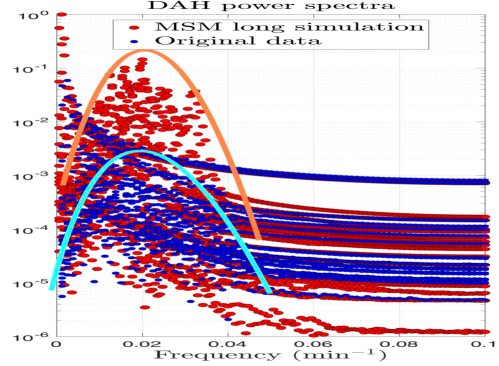
Figure 4: A distinctive broad band peak emerges from long simulations of the data-driven MSM cloud model (3) (marked by the orange curve). The background structure of the DAHD power spectrum from such a simulation agrees to a very good extent with that of the original data (blue vs red dots at higher fequencies). The respective power spectra are normalized to be shown on the same semilogarithmic scale. Note that the DAHD power spectrum is obtained from 1-day observation from the GOES dataset (blue dots), whereas that of the MSM model (red dots), is obtained out of a 100-half-day simulation.

The 100-half-day MSM simulation presents though a broad band peak that emerges over an intermediate frequency band corresponding to the red dots located below the orange curve and above the blue dots in Fig. 4. The question naturally arises whether this predicted energetic bump by the MSM model Eq. (3) over a longer timescale than the available obsevations is of physical relevance or whether this bump corresponds to a model anomaly that calls for its own rectification. A more careful inspection of the DAHD power spectrum from observations seem to indicate though that this bump should correspond to something real as it is sort of latent in the observations (see blue dots below the cyan curve) although not sufficiently energetic to stand out as a bump over a 1-day observation period. To help us draw our conclusion, we analyze next the DAHM patterns associated with this bump.

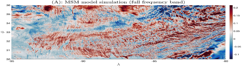
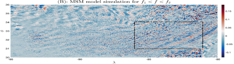
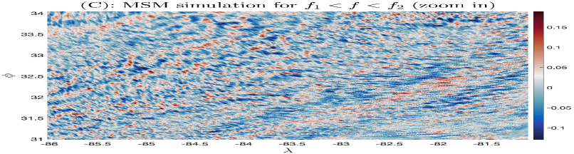
Figure 5: Panel (A): A snapshot of anomaly reflectance field as simulated by the MSM cloud model Eq. (3). The multiscale features of the clouds field are remarkably captured by the MSM cloud model. Panel (B): Here is shown in the physical domain the manifestation, from MSM simulation, of the Harmonic Reconstructed Component given by Eq. (5) associated with the frequency band $f_{1}<f<f_{2}$ corresponding to the bump excess displayed by the DAHD power spectrum (see Fig. 4). Panel (C): Magnification of the black box shown in Panel (B). We observe that individual clouds are arranged along South-West to Norht-East strips, themselves evolving according to a North-West to South-East propagation of gravity waves; see movie in Supporting Information.

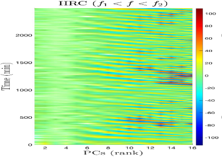
Figure 6: HRC associated with the bump excess visible in Fig. 4 and corresponding to the red dots above the blue ones and below the orange curve. This HRC displays mainly temporal activity from PC₆ to PC₁₆, corresponding, when re-expressed into the physical space according to Eq. (5), to the dynamics of convective inertia gravity waves and that of individual clouds as shown in Fig. 5B and C, respectively. This HRC as computed from the MSM simulation shows the model’s ability to simulate these key organizational features of the cloud field.

VI Simulated Cloud Patterns Analysis

Recall that although cloud street patterns are observed in a recurrent manner over the globe, their lifetime spans at most a few hours [61] that makes their statistical modeling challenging given their multiscale features.

Within this limiting statistical context (short-in-time datasets), a first look at the patterns as simulated by the MSM cloud model (3) (Fig. 5A) suggests the MSM’s ability to capture the clouds’ multiscale features under consideration here. DAHD allows for filtering operations by using the RCs. Such filtering operations are achieved through the calculation of the corresponding Harmonic Reconstructed Component (HRC) which consists essentially to sum up the RCs corresponding to a frequency band of interest [90]. This sum can also be conditioned on a threshold on the magnitude of the corresponding DAHD eigenvalues, as desired, retaining e.g. the most energetic modes within a given frequency band.

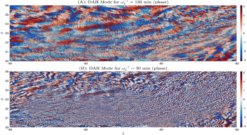
Figure 7: Phase of DAHMs (phase of Eq. (4)) associated with the bump excess shown in Fig. 4. Here the modes shown correspond to the lower and higher frequencies—$130$-min and $30$-min oscillation-period, respectively—over which this bump stretches. The DAHM associated with a $30$-min-period reveals a population of individual clouds while that associated with a $130$-min-period exhibits inertia gravity waves.

For our problem, we are interested in calculating the HRC associated with the energetic bump shown in Fig. 4. To do so, we restrict ourselves to the DAHMs (obtained from MSM simulations) corresponding to the DAHD eigenvalues located on and below the orange curve and above the blue dots. This bump excess lies over the frequency range $(f_{1},f_{2})$, with $f_{1}$ (resp. $f_{2}$) corresponding to an oscillation of $\sim 130$ min (resp. $\sim 30$ min). Figure 6 shows the HRC associated with this bump in the PC-temporal space. Recall that this energetic bump is observed from a (long) simulation of the MSM model (3) (but not from the short-in-time satellite observations), and thus the corresponding HRC is calculated out of the dataset produced from this MSM simulation.

The results shown in Fig. 6 indicate that this HRC displays mainly temporal activity from PC₆ to PC₁₆ in the PC-temporal space. When multiplied by the corresponding EOFs and after summation, we obtain the expression in the physical domain of the HRC, given by

$$\mathcal{H}_{(f_{1},f_{2})}(t,x,y)=\sum_{\ell}\textrm{EOF}_{\ell}(x,y)\textrm{HRC}_{\ell}(t).$$ (5)

For our case study, $\mathcal{H}_{(f_{1},f_{2})}$ captures in a striking way the dynamics of convective inertia gravity waves and of individual clouds lined-up in strips as typically observed in cumulus convection over land [92, 93, 63, 61]; see Fig. 5B and Fig. 5C and the movie available in Supporting Information.

The phase of the DAHMs, obtained by taking the phase of Eq. (4), associated with this HRC, is shown in Fig. 7 for the lower and higher frequencies — $130$-min and $30$-min oscillation period, respectively — over which the energetic bump is stretched in the DAHD power spectrum (see Fig. 4 again). The DAHM associated with a $30$-min-period reveals patterns made of individual clouds (Fig. 7B) while that associated with a $130$-min-period exhibits patterns fingerprinted by inertia gravity waves (Fig. 7A); both of these spatio-temporal scales being consistent with those documented in the literature for shallow Cu and gravity waves [93, 94, 95, 62].

These results re-enforce thus from a higher level of analysis, what was already observed in Fig. 5, namely the MSM model’s ability to simulate convective inertia gravity waves and individual clouds. The energetic bump exhibited by the DAHD power spectrum corresponds thus to a genuine dynamical activity embedded within the shallow cloud field observations from which the MSM model has been designed and learned.

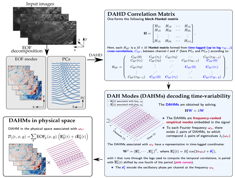
Figure 8: Main steps to extract DAHMs from an EOF decomposition applied to input satellite images. Here the inputs datasets are shown to be the satellite images, but they can be replaced by model’s simulations. The DAHD is applied to the set of PCs either calculated from observations or simulated from the MSM model (3). The resulting multivariate signal has its channels constituted then by such PCs. Recall that the MSM model (3) is a stochastic model of these PCs and as such the latter can be replaced by the simulated PCs to compute the DAHMs from MSM simulations such as shown in Fig. 7.

VII Discussion

Thus, the MSM approach has enabled us to derive a data-driven model of shallow convective clouds, evolving over land. It allows for inferring dynamical equations involving a few variables that are learned from high-resolution satellite observations of continental shallow cumulus. We have shown that, for our problem at hand, low-dimensional linear differential equations that include lagged effects, and are driven by a spatially correlated white noise (see Eq. (3)) are sufficient to provide a reliable model. The resulting MSM cloud model is indeed made of only 32 differential equations driven by white noise that can be easily run on a laptop to produce e.g. a 100-half-day long simulation in only a few seconds.

From a modeling perspective, the frequency ranking property as exhibited by the PCs, with lower frequencies associated with the larger variance content (see PCs shown in Fig. 8), constitutes a key feature for their efficient stochastic modeling by means of such linear MSMs. In contradistinction, an EOF decomposition of rotating stratified turbulent flows leads typically to PCs where each one of them displays a complex mixture of slow and fast frequencies, calling for more sophisticated decomposition and stochastic methods than used here for their efficient modeling; see [20].

The resulting MSM cloud model provides thus a dynamical stochastic generator for the spatio-temporal evolution of the multiscale cloud patterns. This stochastic cloud pattern generator allows us in turn to produce a large ensemble of spatio-temporally coherent patterns and sufficiently diverse statistically to extract dynamical insights about GreenCu that are otherwise difficult to analyze from the raw, short-in-time dataset. The MSM model predicts a broad range of spatio-temporal variability populated by inertia gravity waves as well as demonstrates surprising skills in modeling the individual clouds, as revealed by the DAHD analysis conducted.

Such stochastic emulator abilities open doors for the study of e.g. scaling laws that require typically a large amount of statistics not always available from raw satellite observations. In turn, such types of knowledge gained from MSM simulations is expected to inform and eventually improve comprehensive dynamical models. The approach is obviously not limited to the type of clouds analyzed here, and applications to marine stratocumulus clouds exhibiting other types of coherent structures such as open and closed cells, are planned to be reported elsewhere.

Appendix A GOES–16 ABI dataset and its preprocessing

The dataset used in the present study is the same as analyzed in [62]. We summarize below some elements about this dataset and refer to [62] for more details. The Advanced Baseline Imager (ABI) on board GOES–16 is a state-of-the-art 16-band radiometer, providing four times the spatial resolution, and more than five times faster temporal coverage than the former GOES system [69]. We use the ABI’s level 1B “Red” band (channel 2, $0.64\,\mu m$) radiance, which has the finest resolution (0.5 km) of all ABI bands, over continental US (temporal resolution of 5 minutes). The “Red” band detects reflected visible solar radiation, and its high-resolution makes it ideal for exploring greenCu during daytime. To prepare this dataset for EOF decomposition, we converted the radiance values to reflectance following [96], applied a simple gamma correction to adjust and brighten the images (see below), and reprojected the data from their native geostationary projection into a geographic (latitude–longitude) one. We focus on a vast region of interest (ROI), located between $30^{\circ}N-36^{\circ}N$ and $95^{\circ}W-80^{\circ}W$, on a day that features a typical case of daytime, locally formed shallow convection, from late-morning (10:47 Eastern standard time [EST]) to the afternoon (18:47 EST) of August 22nd, 2018, corresponding to a scalar field comprised of 97, 2D snapshots of corrected reflectance over $1335$ latitude grid points ($\phi$) and 3339 longitude grid points ($\lambda$), for a total of eight hours. The ROI spans two different time zones, such that the local time at the eastern and western parts are four and five hours behind coordinated universal time (UTC), respectively.

Appendix B Gamma correction

The reflectance images obtained from GOES–16 ABI’s “Red” band looked somewhat dark, since the values were in linear units. We adopted thus the common practice which consists of adjusting and brightening the images (before performing the EOF decomposition [62]) by applying a simple gamma correction as follows: $I_{out}=AI_{in}^{\gamma}$, where $I_{in}$ is the darker input image, $\gamma=0.5$, $A=1$, and $I_{out}$ is the adjusted image (corrected reflectance).

Appendix C Learning of the MSM cloud model’s coefficients

In practice, due to shortness in time of the cloud dataset (data collected in the visible from GOES), the estimation of the coefficients in (3) is achieved by means of regularization methods that restrict the learning of the coefficients to a few elements. Several methods exist to do so such as ridge regression, partial-least-square (PLS), or LASSO [97]. Their answers in terms of modeling are however not equivalent [98]. The regularization method along with its parameters are in general selected via cross-validation in which one chooses randomly a subset of the vector time series, applies a given regression technique, and then uses the regression model to reconstruct/predict the segments of the time series that were omitted in the model identification step.

For our dataset, a PLS [99] turns out to be sufficient to calibrate the parameters of the MSM model (3) from the 16 first PCs as extracted from the GOES-16 dataset collected only over the course of 1 day, over continental US. We mention that other approaches such as Kalman filter based algorithms can turn out to be also efficient to estimate the coefficients in presence of short datasets; see e.g. [100, 98]. For both the learning and simulation stages, the MSM model (3) is discretized according to a standard Euler-Maruyama scheme; see e.g. [42].

Appendix D Data-adaptive Harmonic Decomposition (DAHD)

Figure 8 summarizes the main steps, for a given set of PCs, to extract the DAH modes (DAHMs) and obtain their expression in the physical space. Recall that the DAHMs are frequency-ranked empirical modes that come as oscillatory pairs. In fact DAHMs in the physical space can be thought as representing the statistically most relevant and persistent patterns from a singular value decomposition of the estimated cross-spectral density matrix. Rigorous results support this latter statement [90, Theorem V.1]. In this sense, DAHMs closely relate to the spectral EOF modes [101] which operate a similar decomposition of multivariate signals by frequency-ranked empirical modes.

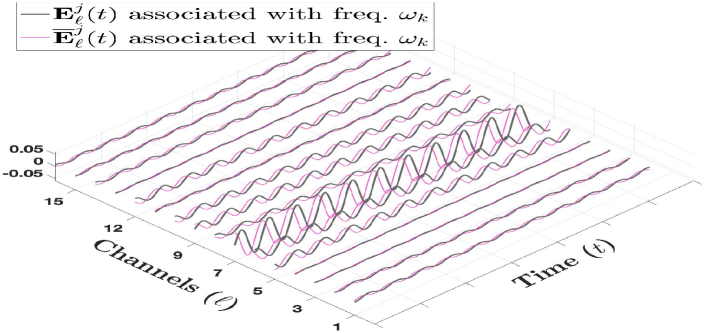
Figure 9: A visualization of a DAHM given by (LABEL:Eq_DAHM); see Text.

By their very construction, the DHAMs form an orthogonal basis and enjoy useful harmonic properties for applications. Indeed, for $\mathbf{X}(t)$ constituted of $L$ channels, each DAHM is naturally associated with a Fourier frequency $\bm{\omega}_{k}$ and has the following representation in time-lagged coordinates [90, Theorem V.1]:

$$\mathbf{W}^{j}=(\mathbf{E}_{1}^{j},\cdots,\mathbf{E}_{L}^{j})^{\mathrm{T}},\mbox{ where }$$ (6)

$$\mathbf{E}_{\ell}^{j}(t)=B_{\ell}^{j}\cos(2\pi\bm{\omega}_{k}t+\bm{\theta}_{\ell}^{j}),$$

with $t$ that runs through the lags used to compute the temporal correlations to form the DAHD correlation matrix; see Fig. 1.

Furthermore, each component, $\mathbf{E}_{\ell}^{j}$, is paired with $\overline{\mathbf{E}}_{\ell}^{j}$ shifted by one fourth of the period; see grey vs pink curves in Fig. 9. For $\mathbf{X}(t)$ constituted of $L$ channels there are exactly $L$ pairs of DAHMs, per Fourier frequency resolved.

The coefficient $B_{\ell}^{j}$ in (LABEL:Eq_DAHM) measures the strength of the frequency $\bm{\omega}_{k}$ in channel $\ell$, for the DAHM $\mathbf{W}^{j}$. The $\bm{\theta}_{\ell}^{j}$ provide the advance or delay of phase between the channels of $\mathbf{W}^{j}$. Figure 9 shows a visualization of the most energetic DAHM pair associated with the dominant frequency expressed in PC₇ for the GOES-16 satellite dataset analyzed in [62] and used in this study as well. Note that this DAHM measures the frequency leakage of that frequency across the channels, here the PCs, and DAHMs do so for any other frequencies and PCs.

References

- Chekroun et al. [2022] M. D. Chekroun, I. Koren, H. Liu, and H. Liu, Science Advances 8, eabq7137 (2022).
- Pavliotis and Stuart [2008] G. A. Pavliotis and A. M. Stuart, Multiscale Methods (Springer, New York, NY, 2008).
- E and Lu [2011] W. E and J. Lu, Scholarpedia 6, 11527 (2011), revision #91540.
- Abdulle et al. [2012] A. Abdulle, E. Weinan, B. Engquist, and E. Vanden-Eijnden, Acta Numerica 21, 1 (2012).
- Kraichnan [1987] R. H. Kraichnan, Complex Systems 1, 805 (1987).
- Kraichnan and Chen [1989] R. H. Kraichnan and S. Chen, Physica D: Nonlinear Phenomena 37, 160 (1989).
- Collins [1985] J. C. Collins, Renormalization (Cambridge University Press, 1985).
- Zwanzig [1961] R. Zwanzig, Physical Review 124, 983 (1961).
- Mori [1965] H. Mori, Progress of Theoretical Physics 33, 423 (1965).
- Hasselmann [1976] K. Hasselmann, Tellus 28, 473 (1976).
- Majda et al. [2001] A. J. Majda, I. Timofeyev, and E. Vanden-Eijnden, Communications on Pure and Applied Mathematics 54, 891 (2001).
- Penland and Sardeshmukh [1995] C. Penland and P. D. Sardeshmukh, Journal of climate 8, 1999 (1995).
- Penland [1996] C. Penland, Physica D 98, 534 (1996).
- Kondrashov et al. [2005] D. Kondrashov, S. Kravtsov, A. W. Robertson, and M. Ghil, J. Climate 18, 4425 (2005).
- Chekroun et al. [2011] M. D. Chekroun, D. Kondrashov, and M. Ghil, Proc. Natl. Acad. Sci. USA 108, 11766 (2011).
- Barnston et al. [2012] A. G. Barnston, M. K. Tippett, M. L. Heureux, S. Li, and D. G. DeWitt, Bull. Am. Meteor. Soc. 93(5), 631 (2012).
- Chen et al. [2016] C. Chen, M. Cane, N. Henderson, D. E. Lee, D. Chapman, D. Kondrashov, and M. D. Chekroun, Journal of Climate 29, 1809 (2016).
- Boers et al. [2017] N. Boers, M. D. Chekroun, H. Liu, D. Kondrashov, D.-D. Rousseau, A. Svensson, M. Bigler, and M. Ghil, Earth Syst. Dynam. 8, 1171 (2017).
- Kondrashov and Berloff [2015] D. Kondrashov and P. Berloff, Geophysical Research Letters 42, 1543 (2015).
- Kondrashov et al. [2018a] D. Kondrashov, M. Chekroun, and P. Berloff, Fluids 3, 21 (2018a).
- Agarwal et al. [2021] N. Agarwal, D. Kondrashov, P. Dueben, E. Ryzhov, and P. Berloff, Journal of Advances in Modeling Earth Systems 13, e2021MS002537 (2021).
- Franzke et al. [2005] C. Franzke, A. J. Majda, and E. Vanden-Eijnden, J. Atmos. Sci. 62, 1722 (2005).
- Franzke and Majda [2006] C. Franzke and A. J. Majda, J. Atmos. Sci. 63, 457 (2006).
- Kondrashov et al. [2006] D. Kondrashov, S. Kravtsov, and M. Ghil, J. Atmos. Sci. 63, 1859 (2006).
- Kondrashov et al. [2013] D. Kondrashov, M. D. Chekroun, A. W. Robertson, and M. Ghil, Geophys. Res. Lett. 40, 5305 (2013), doi:10.1002/grl.50991.
- Chen et al. [2014] N. Chen, A. J. Majda, and D. Giannakis, Geophysical Research Letters 41, 5612 (2014).
- Chen and Majda [2015] N. Chen and A. J. Majda, Monthly Weather Review 143, 2148 (2015).
- Kondrashov et al. [2018b] D. Kondrashov, M. Chekroun, and M. Ghil, Dynamics and Statistics of the Climate System 3, 1 (2018b).
- Kondrashov et al. [2018c] D. Kondrashov, M. D. Chekroun, X. Yuan, and M. Ghil, in Advances in Nonlinear Geosciences, edited by A. Tsonis (Springer, 2018) pp. 179–205.
- Covington et al. [2022] J. Covington, N. Chen, and M. Wilhelmus, Journal of Advances in Modeling Earth Systems 14, e2022MS003218 (2022).
- Chorin et al. [2000] A. J. Chorin, O. H. Hald, and R. Kupferman, Proc. Natl. Acad. Sci. USA 97, 2968 (2000).
- Chorin et al. [2002] A. J. Chorin, O. H. Hald, and R. Kupferman, Physica D 166, 239 (2002).
- Chorin and Hald [2006] A. J. Chorin and O. H. Hald, Stochastic Tools in Mathematics and Science, Surveys and Tutorials in the Applied Mathematical Sciences No. 147 (Springer, New York, 2006).
- Givon et al. [2004] D. Givon, R. Kupferman, and A. Stuart, Nonlinearity 17, R55 (2004).
- Chorin and Stinis [2007] A. Chorin and P. Stinis, Communications in Applied Mathematics and Computational Science 1, 1 (2007).
- Gottwald et al. [2017] G. A. Gottwald, D. T. Crommelin, and C. L. E. Franzke, “Stochastic climate theory,” (Cambridge University Press, 2017) pp. 209–240.
- Lucarini and Chekroun [2023] V. Lucarini and M. Chekroun, arXiv:2303.12009 (2023).
- Chekroun et al. [2021] M. D. Chekroun, H. Liu, and J. C. McWilliams, Proc. Natl. Acad. Sci. USA 118, e2113650118 (2021).
- Chekroun et al. [2017] M. D. Chekroun, H. Liu, and J. C. McWilliams, Computers & Fluids 151, 3 (2017).
- Chekroun et al. [2020a] M. D. Chekroun, H. Liu, and J. C. McWilliams, J. Stat. Phys. 179, 1073 (2020a).
- Majda and Harlim [2013] A. J. Majda and J. Harlim, Nonlinearity 26, 201 (2013).
- Kondrashov et al. [2015] D. Kondrashov, M. D. Chekroun, and M. Ghil, Physica D 297, 33 (2015).
- Falkena et al. [2019] S. Falkena, C. Quinn, J. Sieber, J. Frank, and H. Dijkstra, Proceedings of the Royal Society A 475, 20190075 (2019).
- Wouters and Lucarini [2012] J. Wouters and V. Lucarini, J. Stat. Mech.: Theory Experiment , P03003 (2012).
- Wouters and Lucarini [2013] J. Wouters and V. Lucarini, J. Stat. Phys. 151, 850 (2013).
- Chorin and Lu [2015] A. J. Chorin and F. Lu, Proc. Natl. Acad. Sci. USA 112, 9804 (2015).
- Lu et al. [2017] F. Lu, K. K. Lin, and A. J. Chorin, Physica D: Nonlinear Phenomena 340, 46 (2017).
- Nastrom and Gage [1985] G. D. Nastrom and K. S. Gage, Journal of the atmospheric sciences 42, 950 (1985).
- Stinis [2007] P. Stinis, Multiscale Model. & Simul. 6, 741 (2007).
- Lin and Lu [2021] K. K. Lin and F. Lu, Journal of Computational Physics 424, 109864 (2021).
- Lei et al. [2016] H. Lei, N. Baker, and X. Li, Proceedings of the National Academy of Sciences 113, 14183 (2016).
- Brennan and Venturi [2018] C. Brennan and D. Venturi, Journal of Computational Physics 372, 281 (2018).
- Wang et al. [2020] Q. Wang, N. Ripamonti, and J. S. Hesthaven, Journal of Computational Physics 410, 109402 (2020).
- Gupta and Lermusiaux [2021] A. Gupta and P. F. J. Lermusiaux, Proceedings of the Royal Society A 477, 20201004 (2021).
- Kravtsov et al. [2005a] S. Kravtsov, D. Kondrashov, and M. Ghil, Journal of Climate 18, 4404 (2005a).
- Santos Gutiérrez et al. [2021] M. Santos Gutiérrez, V. Lucarini, M. D. Chekroun, and M. Ghil, Chaos 31, 053116 (2021).
- Zhu et al. [2018] Y. Zhu, J. Dominy, and D. Venturi, Journal of Mathematical Physics 59, 103501 (2018).
- Nair et al. [1998] U. Nair, R. Weger, K. Kuo, and R. Welch, Journal of Geophysical Research: Atmospheres 103, 11363 (1998).
- Heus and Seifert [2013] T. Heus and A. Seifert, Geoscientific Model Development 6, 1261 (2013).
- Stevens et al. [2019] B. Stevens, S. Bony, H. Brogniez, L. Hentgen, C. Hohenegger, C. Kiemle, T. S. L’Ecuyer, A. K. Naumann, H. Schulz, P. A. Siebesma, et al., Quarterly Journal of the Royal Meteorological Society , 1 (2019).
- Dror et al. [2020] T. Dror, I. Koren, O. Altaratz, and R. H. Heiblum, IEEE Transactions on Geoscience and Remote Sensing (2020).
- Dror et al. [2021] T. Dror, M. D. Chekroun, O. Altaratz, and I. Koren, Atmos. Chem. Phys. 21, 12261 (2021).
- Da Silva et al. [2011] R. R. Da Silva, A. W. Gandu, L. D. Sá, and M. A. S. Dias, Biogeochemistry 105, 201 (2011).
- Dror et al. [2022] T. Dror, V. Silverman, O. Altaratz, M. D. Chekroun, and I. Koren, Geophysical research letters 49, e2021GL096684 (2022).
- Bony [2005] S. Bony, Geophysical Research Letters 32 (2005).
- Webb et al. [2006] M. J. Webb, C. Senior, D. Sexton, W. Ingram, K. Williams, M. Ringer, B. McAvaney, R. Colman, B. J. Soden, R. Gudgel, et al., Climate Dynamics 27, 17 (2006).
- Vial et al. [2017] J. Vial, S. Bony, B. Stevens, and R. Vogel, in Shallow Clouds, Water Vapor, Circulation, and Climate Sensitivity (Springer, 2017) pp. 159–181.
- Nuijens and Siebesma [2019] L. Nuijens and A. P. Siebesma, Current Climate Change Reports 5, 80 (2019).
- Schmit et al. [2017] T. J. Schmit, P. Griffith, M. M. Gunshor, J. M. Daniels, S. J. Goodman, and W. J. Lebair, Bulletin of the American Meteorological Society 98, 681 (2017).
- Preisendorfer and Mobley [1988] R. W. Preisendorfer and C. D. Mobley, Developments in Atmospheric Science 17 (1988).
- Villermaux [1995] E. Villermaux, Physical Review Letters 75, 4618 (1995).
- Tziperman et al. [1994] E. Tziperman, L. Stone, M. A. Cane, and H. Jarosh, Science 264, 72 (1994).
- Roques et al. [2014] L. Roques, M. D. Chekroun, M. Cristofol, S. Soubeyrand, and M. Ghil, Proc. R. Soc. A 470, 20140349 (2014).
- Keane et al. [2017] A. Keane, B. Krauskopf, and C. M. Postlethwaite, Chaos: An Interdisciplinary Journal of Nonlinear Science 27, 114309 (2017).
- Chekroun et al. [2018] M. D. Chekroun, M. Ghil, and J. D. Neelin, in Advances in Nonlinear Geosciences, edited by A. Tsonis (Springer, 2018) pp. 1–33.
- Koren and Feingold [2011] I. Koren and G. Feingold, Proc. Natl. Acad. Sci 108, 12227 (2011).
- Koren et al. [2017] I. Koren, E. Tziperman, and G. Feingold, Chaos: An Interdisciplinary Journal of Nonlinear Science 27, 013107 (2017).
- Chekroun et al. [2020b] M. D. Chekroun, I. Koren, and H. Liu, Chaos 30, 053130 (2020b).
- Kravtsov et al. [2005b] S. Kravtsov, D. Kondrashov, and M. Ghil, Journal of Climate, J. Climate 18, 4404 (2005b).
- Granger [1969] C. W. Granger, Econometrica: Journal of the Econometric Society , 424 (1969).
- Broomhead and King [1986] D. S. Broomhead and G. P. King, Physica D 20, 217 (1986).
- Vautard and Ghil [1989] R. Vautard and M. Ghil, Physica D 35, 395 (1989).
- Ghil et al. [2002] M. Ghil, M. R. Allen, M. D. Dettinger, K. Ide, D. Kondrashov, M. E. Mann, A. W. Robertson, A. Saunders, Y. Tian, F. Varadi, and P. Yiou, Rev. Geophys. 40, 1 (2002).
- Brunton et al. [2021] S. L. Brunton, M. Budišić, E. Kaiser, and J. N. Kutz, arXiv preprint (2021).
- Williams et al. [2015] M. O. Williams, I. G. Kevrekidis, and C. W. Rowley, Journal of Nonlinear Science 25, 1307 (2015).
- Kutz et al. [2016] J. N. Kutz, S. L. Brunton, B. W. Brunton, and J. L. Proctor, Dynamic Mode Decomposition: Data-driven Modeling of Complex Systems (SIAM, 2016).
- Klus et al. [2018] S. Klus, F. Nüske, P. Koltai, H. Wu, I. Kevrekidis, C. Schütte, and F. Noé, Journal of Nonlinear Science 28, 985 (2018).
- Froyland et al. [2021] G. Froyland, D. Giannakis, B. Lintner, M. Pike, and J. Slawinska, Nature Communications 12, 1 (2021).
- Froyland et al. [2007] G. Froyland, K. Padberg, M. England, and A. Treguier, Physical Review Letters 98, 224503 (2007).
- Chekroun and Kondrashov [2017] M. D. Chekroun and D. Kondrashov, Chaos 27, 093110 (2017).
- Zhen et al. [2022] Y. Zhen, B. Chapron, E. Mémin, and L. Peng, Physical Review E 105, 034205 (2022).
- Plank [1966] V. G. Plank, Tellus 18, 1 (1966).
- Plank [1969] V. G. Plank, Journal of Applied Meteorology and Climatology 8, 46 (1969).
- Jiang et al. [2006] H. Jiang, H. Xue, A. Teller, G. Feingold, and Z. Levin, Geophysical Research Letters 33 (2006).
- Lane [2015] T. P. Lane, in Encyclopedia of Atmospheric Sciences (2nd Edition) (Elsevier, 2015) pp. 171–179.
- Schmit et al. [2010] T. Schmit, M. Gunshor, G. Fu, T. Rink, K. Bah, and W. Wolf, GOES-R Advanced Baseline Imager (ABI) Algorithm Theoretical Basis Document for: Cloud and Moisture Imagery Product (CMIP) (University of Wisconsin–Madison, 2010).
- Hastie et al. [2009] T. Hastie, R. Tibshirani, and J. Friedman, Linear Methods for Regression (Springer, 2009).
- Strounine et al. [2010] K. Strounine, S. Kravtsov, D. Kondrashov, and M. Ghil, Physica D 239, 145 (2010).
- Abdi [2003] H. Abdi, Encyclopedia for Research Methods for the Social Sciences 6, 792 (2003).
- Harlim and Li [2015] J. Harlim and X. Li, Physical Review E 91, 053306 (2015).
- Schmidt et al. [2019] O. Schmidt, G. Mengaldo, G. Balsamo, and N. Wedi, Monthly Weather Review 147, 2979 (2019).