Parameterized Learning and Feature Distillation with Synthetic Training Data

Abstract

Spectral methods, employed in numerical simulations and big-data analytics, leverage modal or nonlocal representations of data. Here, we validate a spectral-methods paradigm with a hybrid encoded diffraction system where the electronic model learns a truncated set of optical pattern correlations. In a demonstration, we implement a speckle image training basis. Both the training dataset and the transferred learning are parameterized with Singular-Value Decomposition Entropy ($H_{SVD}$) and Speckle-Analogue Density (SAD), which are proxies for the image complexity and neural network convergence rate ($H_{SVD}$), and structurally similar image reconstruction (SAD). Notably, our spectral-methods approach achieves feature distillation: with CIFAR-100 images reconstructed with high-$H_{SVD}$ modes, we achieve classification accuracies of 60% (a result that rivals state-of-the-art computer algorithms from a decade ago). Our parameters illustrate that the most faithfully reproduced images are not the ones that are the most accurately classified. Additionally: complex images may be analyzed with simple neural-network models that are trained with high-$H_{SVD}$ synthetic data. Our work highlights new opportunities for pipelines based on simple electronic models that learn from tailored, synthetic training data. Code is available at: https://github.com/altaiperry/Reconstruction23_Perry

1 Introduction

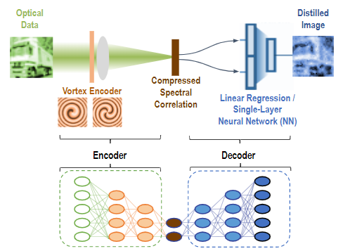
Figure 1: Schematic for a vortex, optically coded, electronically decoded system. Truncated or compressed set of spectral correlations are produced in the sensor plane (top). This system is analogous to an autoencoder, machine-learned architecture that distills features and denoises images (below).

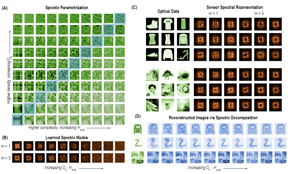
Figure 2: (A) Representative speckle images from 100 training sets and models, which are parameterized with Singular Value Decomposition Entropy ($H_{SVD}$) and Speckle Analogue Density (SAD, $\Omega_{k}$). The diagonal, blue-highlighted images represent the primary dataset from which the other 90 are formed. (B) Representative vortex-encoded sensor patterns with topological charges $m$ = 1,3 for the primary dataset. (C) Images from the MNIST fashion and CIFAR-100 datasets and their vortex-encoded, sensor patterns for $m=1,3$. (D) Representative reconstructed images using the pre-trained models from the primary datasets.

The concept of superposition is a fundamental principle in physics that is applied to spectral computational methods [1, 2, 3]. With spectral methods, data is mapped through a linear transformation to a distribution associated with polynomials or modal functions [4]. This approach is extended to unsupervised machine learning [5, 6]. Spectral representations offer the opportunity to compress vast, multi-dimensional volumes of information into smaller sets of physically interpretable quantities related to system- or user-defined relations. Analytic, compressed representations offer robust and reliable algorithms for the simulation of complex systems.

Spectral representations are leveraged with encoded wave propagation [7, 8, 9, 10], optical neural networks [11, 12, 13, 14, 15, 16, 17, 18, 19, 20, 21, 22, 23], and next-generation computational cameras [24, 25, 26, 27, 28]. Such hybrid optical-electronic systems show potential for high-speed/low-power computing and enhanced image processing, however the electronic sensing of optical fields, which loses phase information, limits the ability to reconstruct the signal. Phase information is lost by amplitude-only sensor measurements; instead of the linear weights of a signal basis, the sensor provides a correlation. This loss of phase information presents ambiguity in the design of downstream algorithms (such as pattern recognition, feature distillation, and image classification).

In this Article, we map sensor and signal data with a learned, linear transformation and validate a spectral-methods paradigm for optical neural networks. While the way to characterize such a linear transformation would generally require a maximum number of training images equal to the number of target-image pixels, such a linear-superposition approach does not work since the sensor images are nonlinear interference patterns and correlations, which omit phase information. It has been shown that this inverse transformation between sensor and signal images may be learned with Tikhonov or Ridge regularization [29], however such regularization is not required in a vortex-encoded, Fourier-optics system. The learned correlations determine the eigenimages that shape image reconstruction. The hybrid system is analogous to an autoencoder architecture that incorporates optical encoding and electronic decoding [Fig. 1]. Such a framework distills features, which we demonstrate with a speckle-spectral training dataset approach, image reconstruction, and subsequent classification.

We construct ‘span-encoded’ speckle data, where the relative span is defined by singular value decomposition (SVD) [30, 31, 32] and analyze the NN weights from the trained models. Speckles are a tractable image basis that are observed in a variety of imperfect, coherent-imaging systems [33, 34, 35]. The NN weights connect the learned model’s single-pixel response with its learned features, structural similarity (SSIM) [36], and post-processing classification accuracy.

Remarkably, the models that learn data-agnostic speckle correlations distill patterns and provide decent classification of CIFAR-100 and other datasets. In other words, even when the goal images do not contain human-recognizable features, their learned correlations aid image classification. The local features are human-recognizable patterns and textures and are what convolutional NNs identify. By contrast, global features correlate to the eigenmodes of the system, which are not guaranteed to be human-recognizable [37]. Our work highlights the efficiency of the simplest vortex-encoded optical neural networks and explores their capacity appropriate for real-time applications.

2 Results

2.1 Vortex-Encoded Polynomial Field Gradients

Encoded diffraction introduces a mask $M(x,y)$ that shapes the sensed patterns and regularizes the phase retrieval problem. The sensor field pattern ${\psi}_{o}^{\prime}(u,v)$ is proportional to the Fourier transform of the field before the lens aperture $\psi(x,y)$, where the transform pairs are $(x,y)\leftrightarrow(u,v)$ [7]. A combination of Fresnel and Fourier-plane imaging may also offer more information at the sensor [20]. The inverse phase problem becomes

$$\left|\psi_{m}^{\prime}\right|=|\mathcal{F}\left(M\cdot\psi\right)|\longrightarrow\psi,$$ (1)

where ($\cdot$) denotes the element-wise Hadamard product. We implement coded diffraction with the vortex phase encoder,

$$M(x,y)\propto e^{\pm im\phi},$$ (2)

where $r$ and $\phi$ are the radial and azimuthal coordinates in the aperture plane. The positive value of the topological charge is $m$ with $\pm$-sign. The vortex encoder produces the field gradient patterns in the Fourier-transformed sensor plane [14]:

$$\psi^{\prime}_{\pm m} \propto \mathcal{F}\left\{M(x,y)\psi(x,y)\right\}$$ (3)

$$\approx \left[\left(\pm\partial_{v}-i\,\partial_{u}\right)\right]^{m}\psi_{o}^{\prime},$$ (4)

where $\partial_{u}$ and $\partial_{v}$ are the partial derivatives with respect to $u$ and $v$ (and where $u$ and $v$ are the transverse coordinates in the sensor plane.

The sensor intensity pattern from a vortex encoder carries a polynomial gradient representation, which we present here in closed form:

$$\mathcal{X} = |\psi^{\prime}_{m}|^{2}$$

$$\propto \sum_{{j,k,l_{1},l_{2}}\atop{j+k+l_{1}+l_{2}=m}}s_{j,k,l_{1},l_{2}}\,\left[\partial_{u}^{k+l_{1}}\partial_{v}^{j+l_{2}}\psi_{o}^{\prime}\right]\;\left[\partial_{u}^{k+l_{2}}\partial_{v}^{j+l_{1}}{\psi_{o}^{\prime}}^{*}\right]$$

with linear weighting coefficients:

$$s_{j,k,l_{1},l_{2}}=\frac{m!}{j!\,k!\,l_{1}!\,l_{2}!}\,\left(\pm i\right)^{l_{1}+l_{2}}\left(-1\right)^{l_{2}}.$$ (6)

Equation 2.1 identifies the vortex-encoded sensor pattern as a superposition of gradient correlations of the unencoded Fourier-plane field $\psi_{o}^{\prime}$ and its complex conjugate, $\psi_{o}^{\prime*}$. On axis, the vortex encoder provides some degree of shape compression [38].

This map between signal fields and sensor intensity patterns is the solution from a 2-D polynomial regression problem of order $2m$, the solution of which is approximated by simple NNs [39, 40, 41]. To solve the inverse problem [Eq. 1] for both real and imaginary parts of $\psi^{\prime}_{m}$, two vortex encoders are needed (in our case, $m$ = $1,3$).

The interpolation of $\psi$ from $|\psi^{\prime}_{m}|^{2}$ ($|\psi^{\prime}_{m}|^{2}\rightarrow\psi$) involves the calculation or inference of $\nabla\psi^{\prime}_{o}\rightarrow\psi^{\prime}_{o}$ and $\psi^{\prime}_{o}\propto\mathcal{F}\psi\rightarrow\psi$. In fact, when $m=0,\pm 1$, then the sensor patterns provide a quadratic relation for the gradient of $\psi_{o}^{\prime}$, which is accurately solved by a single-layer NN without hidden layers [39]. Higher values of $m$ provide additional terms in Eq. 2.1 to fit $\nabla\psi_{o}^{\prime}$, which yield higher accuracies (as with a Taylor expansion) at the cost of deeper calculations.

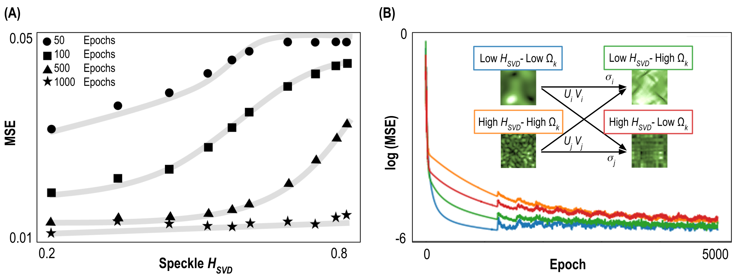
Figure 3: (A) Mean-Squared Error (MSE) during NN training for ten generated models with different $H_{SVD}$ at 50, 100, 500 and 5000 epochs. The constant-time MSE curves (isochrones) converge to similar MSE, however the higher-$H_{SVD}$ models take longer to converge. (B) Log-loss (log(MSE)) convergence of four models trained with different datasets with swapped singular values ($\sigma_{i}$): $\bar{H}_{SVD}(low)=0.3$; $\bar{H}_{SVD}(high)=0.75$. While the training eigenimages $U_{i}\,V_{i}$ or $U_{j}\,V_{j}$ affect the learning rate, the $H_{SVD}$ has a stronger effect on the learning rate.

2.2 Parameterized Image Reconstruction

When the signal is reconstructed from sensor intensity measurements, we can adopt a regression-based spectral methods approach that incorporates soft-target images. One of this Article’s primary contributions is the analysis of soft-target goal or training images parameterized by a “virtual channel width”—i.e., the information transferred per shot. This virtual channel width is associated with SVD entropy, $H_{SVD}$:

$$H_{SVD} = \frac{-1}{\log_{2}N}\sum^{N}_{i}\tilde{\sigma}_{i}\log_{2}\tilde{\sigma}_{i}$$ (7)

$$\tilde{\sigma}_{i} = \frac{\sigma_{i}}{\sum_{j}^{N}\sigma_{j}}$$ (8)

where $\sigma_{i}$ is the $i^{th}$ singular value (SV) and $N\times N$ is the dimension of the image. Our definition [Eq. 8] yields values of $H_{SVD}$ with a range of (0,1] and in contrast to prior work [42], we use linear values of $\sigma_{i}$ to signify a measure of the electric field rather than photon probabilities [43]. Our measure $H_{SVD}$ is analogous to the 1-D measure of Shannon information, where the accurate transmission of higher-entropy signals requires more bits [44]. Shannon information is insufficient to capture 2-D image complexity [45] since a shuffle of image pixels yields the same Shannon entropy.

$H_{SVD}$ is a relative measure of bandwidth or image span [46]; larger values of $H_{SVD}$ signify that more eigenimages are needed to approximate an image. $H_{SVD}$ is also a stopping measure or figure of merit for Deep-NN image reconstruction [47], a measure of self-similar fractals [43], and a measure of the distribution of electric-field modes in an optical system [48, 34].

We create 10 datasets of 10k $32\times 32$ px speckle patterns as training data $\mathbf{\Psi}_{train}$,

$$\mathbf{\Psi}_{\rm train}^{(\gamma)}(x,y)=\Re\left[\mathcal{F}^{-1}\left\{(k_{x}^{2}+k_{y}^{2})\gamma e^{-(k_{x}^{2}+k_{y}^{2})\gamma+2\pi i\mathbf{\Lambda}}\right\}\right]$$ (9)

where the spatial frequencies $k_{x}$ and $k_{y}$ are limited to the range: $[-k_{\rm max},k_{\rm max})$, $\gamma$ is a tunable density parameter and $\Lambda$ is a $32\times 32$ random array with uniform distribution between [0,1]. These training patterns are motivated by the Fresnel propagation of the second-order statistics of a randomly scattered beam [49] and are parameterized by $H_{SVD}$ and Speckle Analogue Density (SAD).

SAD refers to the root mean-squared spatial frequency, $\Omega_{k}$, or

$$\Omega_{k}=\frac{\sqrt{\langle k_{x}^{2}\rangle+\langle k_{y}^{2}\rangle}}{k_{\rm max}}.$$ (10)

The values of SAD, $\Omega_{k}$, like $H_{SVD}$, have a range of (0, 1]. Given the explicit equation for the generated test datasets in Eq. 9,

$$\Omega_{k}=\frac{1}{k_{\rm max}}\sqrt{\frac{2}{\gamma}}.$$ (11)

In total, 100 NN models are trained, each from 100, 10k-image datasets [Fig. 2(A)]. The ten primary speckle training sets are subsequently used to generate the additional 90 by switching the eigenimages and eigenvalues. Each set of images is used to train a no-hidden-layer NN with linear activation and no bias. The resulting model is a linear transformation of the form,

$$\mathbf{\Psi}_{pred}=\mathcal{X}\mathbf{W}^{T},$$ (12)

where $\mathbf{\Psi}_{pred}$ is the approximated original image, $\mathcal{X}$ is the sensor plane intensity [Eq. 2.1] and $\mathbf{W}^{T}$ are the weights of the derived model. Since we use a single layer NN, these weights are the inverse linearized transfer function that solves Eq. 1.

2.3 $H_{SVD}$ and SAD as Learning and SSIM Indicators

The NNs trained with higher average $H_{SVD}$ images take longer to converge. We preform the training with randomly generated training sets of similar $H_{SVD}$ and SAD ($\Omega_{k}$) statistics and run experiments in triplicate. Figure 3(A) shows 10 models’ MSE at four slices of time. Each model’s MSE is plotted against the average $H_{SVD}$ of the model’s training data. Across randomized triplicate training sets, the measured accuracy at analyzed ‘stopping points’ has a variance of less than $10^{-5}$ per pixel, which indicates that the epoch-on-epoch convergence profiles are reproducible [Fig. 3(B)].

To explain the relationship between $H_{SVD}$ and convergence time, we calculate the epoch-on-epoch $\Delta L$, the epoch-by-epoch change in loss through gradient descent. Let $\mathcal{X}_{k}W_{n}^{T}$ be the reconstructed images produced by the NN transformation preformed on a dataset $\mathbf{\Psi}$ that consists of $N$ Fourier intensity patterns. The mean square error loss over $K$ images at epoch $n$ is:

$$L_{n}=\sum_{k}^{K}(\mathbf{\Psi}_{k}-\mathcal{X}_{k}W_{n}^{T})^{T}(\mathbf{\Psi}_{k}-\mathcal{X}_{k}W_{n}^{T}).$$ (13)

where $n$ denotes the individual epoch, and $k$ denotes the individual image, $K$ is the total number of images, $W$ is the derived weights matrix, and $\alpha$ is the learning rate constant. It can be shown that the loss-on-loss change is:

$$\Delta L_{n,k}\frac{K}{2\alpha}=\mathcal{X}_{k}W_{n}^{T}\epsilon_{n,k}\mathcal{X}_{k}\mathcal{X}_{k}^{T}+W_{n}\mathcal{X}_{k}^{T}\mathcal{X}_{k}\mathcal{X}_{k}^{T}\epsilon_{n,k}.$$ (14)

This expression, Eq. 14, is proportional to the error, $\epsilon_{n,k}$. Equation 14 is smaller for matrices with a slow SV drop off or high $H_{SVD}$ and large relative span. A higher convergence time is attributed to lower epoch-to-epoch change in loss governed by the epoch-to-epoch error. Images whose eigenimages are weighted more evenly and carry higher $H_{SVD}$ are less easily learned.

This trend is dependent on the $H_{SVD}$ regardless of the dataset eigenimages. High $H_{SVD}$ training data yields lower NN learning rates regardless of the SAD ($\Omega_{k}$). To illustrate that the learnability is associated with $H_{SVD}$ rather than the eigenimages, we swap eigenimages and SVs in the training dataset generation and compare the model convergence rates [Fig. 3(B)]. The models trained with higher-$H_{SVD}$ data converges more slowly.

In contrast, SAD parity is a heuristic for structurally similar reconstruction. SAD parity refers to similar $\Omega_{k}$ in the train and test data. From each of the models visualized in Fig. 2(B), we calculate the SSIM with the CIFAR-100 dataset. The colored dots show the average SSIM while background contour shows the histogram of the CIFAR-100 test dataset’s $H_{SVD}$ and $\Omega_{k}$ [Fig. 4]. While the $H_{SVD}$ has a direct impact on training time, it has little-to-no impact on reconstruction accuracy; instead, SAD parity between training and test datasets dictates reconstruction accuracy.

The peak in SSIM vs. SAD on the right of Fig. 4(A) is not symmetric: models produced with lower-SAD training images have higher SSIM than the models produced with higher-SAD training images. This is largely a result of the SSIM metric: smooth, shape-aligned images have higher SSIM [36]. By contrast, the images generated by models with high SAD training data are more visually-dense and have lower SSIM. Not surprisingly, the models that are trained with similar-SAD images also generate images with low MSE. These trends relating the statistics of the CIFAR-100 dataset SAD and $H_{SVD}$ to the reconstructed MSE and SSIM are observed with the MNIST Digit, Fashion, and CIFAR-10 datasets.

These trends may be applied to maximize image reconstruction quality with minimal training time. For example, synthetic training data can be chosen to provide a ‘good-enough’ standard of image reconstruction or SSIM rather rather than pixel-for-pixel fidelity (MSE). A training dataset chosen with similar SAD will provide high SSIM and such a training set can be chosen to have low-$H_{SVD}$ so that the model converges faster.

We further investigate the encoded feature distillation using the model weights ($\mathbf{W}^{T}$) as an inverse transfer function [Eq. 12]. We visualize the impulse response of this linear transfer function or the single pixel response (SPR) for our models. In Fig. 4(B), we plot the SPRs for the 10 primary models. The expected SPR patterns are described by $\mathcal{X}$ in Eqs. 4 and 2.1 where $\mathcal{X}$ contains one non-zero pixel.

Each reconstructed sensor-plane image exhibits spiral fringes that reveal the vortex-encoded field phase curvature associated with $M(x,y)$. The corresponding fringes are more closely spaced for an off-axis pixel than they are for an on-axis pixel. As a result, the SPR of the central pixel is accurately reconstructed with intermediate $H_{SVD}$ and SAD values. In contrast, the SPR of off-axis pixels are accurately reconstructed with higher $H_{SVD}$ and higher-SAD models.

To summarize, within a speckle training framework parameterized with $H_{SVD}$ and SAD,

• The $H_{SVD}$ of the sensor training images are associated with the NN learning rate. (Models trained with high-$H_{SVD}$ patterns converge more slowly.)

• The SAD of the training images provides a threshold for self-similar image reconstruction. (The SAD of the training dataset should match the SAD or be lower than that of the reconstructed image.)

• In a vortex-encoded, lensed system, the feature reconstruction depends on the feature location and phase at the sensor plane. (i.e., higher $H_{SVD}$ and SAD training are generally needed to reproduce off-axis features.)

2.4 Feature Distillation with Speckle Decomposition

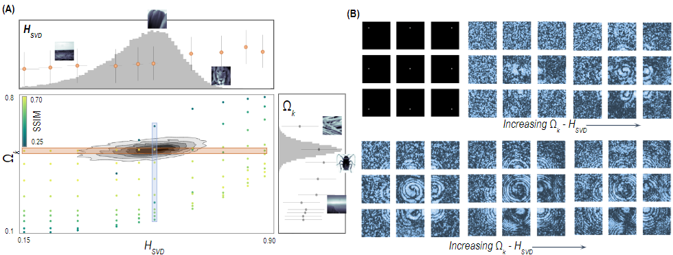
Figure 4: (A) A 2-D histogram of $\Omega_{k}$ and $H_{SVD}$ for the images in the CIFAR-100 dataset. The top and right show 1-D histograms of $H_{SVD}$ and $\Omega_{k}$, respectively. Colored markers and range bars indicate the average Structural Similarity Index Metrics (SSIMs) of the reconstructed CIFAR-100 images by pre-trained models with average speckle $(H_{SVD},\Omega_{k})$. (B) Input single pixel images or single pixel responses for 5 of the original 10 speckle datasets with $(H_{SVD},\Omega_{k})$ = $(0.19,0.062)$, $(0.33,0.081)$, $(0.49,0.14)$, $(0.63,0.24)$ and $(0.78,0.39)$. As both $H_{SVD}$ and $\Omega_{k}$ increase, the outer-pixel, fringe patterns are better resolved at the expense of the center-pixel features.

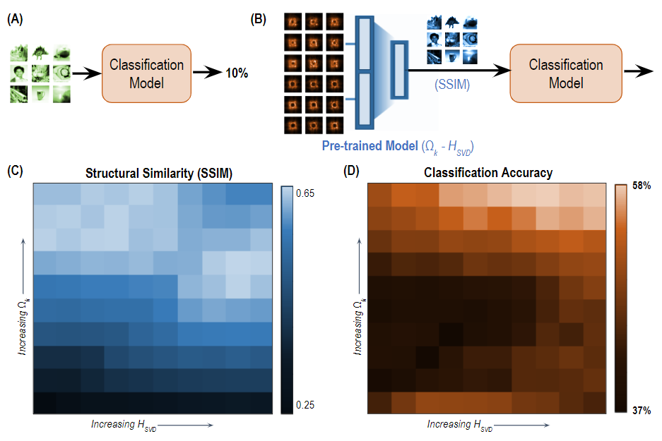
Figure 5: Workflow of (A) conventional classification with ground truth images as inputs and (B) filtered classification with reconstructed images from a pre-trained model as inputs. (C) The Structural Similarity Index Metric (SSIM) and (D) the classification accuracy of reconstructed images with the workflow in (B). Each square is the average SSIM/classification accuracy for CIFAR-100 when trained on a pre-trained model with speckle images of $H_{SVD}$ and $\Omega_{k}$. Note that the highest reconstruction accuracy is achieved with $H_{SVD}$ speckles and is 58%. Meanwhile, the same classification model, i.e., the workflow in (A), yields an accuracy of 10%.

Surprisingly, the most faithfully recreated images are not the most well classified. We use reconstructed CIFAR-100 images from all 100 models and subsequently classify with a 2-layer NN [Fig. 5(A-B)]. The SSIM of the reconstructed images are shown in Fig. 5(C), and their classification accuracies are shown in Fig. 5(D). Models trained with higher-SAD data generate images that are classified best after image reconstruction. The results are not specific to CIFAR-100; results with other datasets show similar trends.

Our results show prominent feature distillation through image reconstruction: a simple NN classifies the original CIFAR-100 with accuracies of 10%, while the same NN classifies the imperfectly-reconstructed images from speckle-trained models with accuracies upwards of 58%. Results for MNIST handwritten digits, MNIST Fashion, and CIFAR-10 datasets are provided in the Appendix. Note that this CIFAR-100 classification accuracy with a shallow NN, in fact, rivals the performance of Deep NNs that, ten years ago, were state of the art [50]. This curious behavior of our image reconstruction–the learned feature reconstruction from compressed spectral correlations– is akin to the ‘distillation’ of Deep NN information [51].

3 Discussion

Our research addresses topics of interest to the machine-learning community related to model learning rate, model convergence, feature distillation and reconstruction accuracy [52, 53, 54, 51]. We have discovered that, rather than calculating the image priors via optimization or learning local features à la convolutional NN, we can instead guess at what spectral or global features exist in a class of images and encode them in a generalized synthetic training dataset a priori.

The advantage of our physically realized optical-electronic autoencoder system is that it is tractable, simple, carries low computational overhead but mirrors and expands on successful computer vision algorithms. For example, similar nonlocal motifs in NNs have been quantified and shown to hamper classification schemes using convolutional NNs only, which is why Krizhevsky introduces a whitening transform that subsequently and selectively discards features [53].

The strength and potential drawback of hybrid systems lies in the simultaneous operations of both convolutions and filters with the optical preprocessing. That is, given a set of training images, a NN is presented with the sensor patterns, which are a truncated set of spectral correlations that pre-define the pattern-basis-vectors. These eigenimages are analogous to the filters of the whitening transform. With better understanding of the encoded motifs beyond textures, shapes, and edges, features (i.e., the kernels of convolutional NNs) could be designed into the synthetic training data.

In conclusion, we have demonstrated a facile spectral-methods approach to analyze how learning is transferred. With vortex encoders, it can be shown that a NN efficiently learns the compressed spectral correlations of global features and subsequently, it learns a generalized linear map between signal field and sensor intensity measurements. While other encoders may generalize in a similar way, vortex patterns are mostly smooth and will minimize the $H_{SVD}$ of the sensor pattern, which will generally reduce the model training time.

While the current approach with machine-learning neural networks involves training and testing with similar data, we generate and compare models that are parameterized by their synthetic training data. The parameterized, learned models provide filtered inputs for downstream classification. Surprisingly, with high $H_{SVD}$ speckle training data, we achieve accuracies of 58% with CIFAR-100 using a simple, 2-layer shallow classification model.

As our work has shown, there are trade-offs with this approach to feature distillation, since a higher-span dataset as characterized by $H_{SVD}$ generally exhibits a reduced learning rate. However, this carries strong analogies to teaching and learning in humans [55, 56]. Extended further, our work may contribute to a unified system of machine learning design that also integrates how one recognizes features to the statistical-weighted exposure to training data.

4 Appendix

4.1 Training Time Dependence on Span

This derivation indicates that the datasets with higher $H_{SVD}$ take longer to train in a single layer neural network. We start with the transformation preformed on a data set $\psi$ consisting of $N$ images. The image captured on a camera sensor at the focal plane is given by the intensity pattern of the Fourier transform of the electric field. We denote this electric field as the Hadamard (or element-wise) product of ’mask’, $M$, with each image in $\psi$. The resulting image is denoted by $\psi^{\prime}$,

$$\psi^{\prime}=\left(\mathcal{F}(M\cdot\psi)\right)^{*}\left(\mathcal{F}(M\cdot\psi)\right)$$ (15)

If $\psi^{\prime}$ is defined as above and ground truth is $\psi$, we can define mean square error loss over $K$ images as at epoch $n$,

$$L_{n}=\sum_{k}^{K}(\psi_{k}-\psi^{\prime}_{k}W_{n}^{T})^{T}(\psi_{k}-\psi^{\prime}_{k}W_{n}^{T}).$$ (16)

Stepping forward with the method of gradient descent yields an epoch-on-epoch loss difference. While the stochastic gradient descent optimizer (i.e., adam) used in this investigation will adjust the learning rate, $\alpha$, to avoid small local minimums, the gradient in loss is largely given by the data manifold. The gradient descent algorithm discovers the next $W$ via

$$W_{n+1}=W_{n}-\alpha\frac{\partial L_{n}}{\partial W_{n}}.$$ (17)

Substituting Eq. 16 into Eq. 17 yields

$$W_{n+1}={W_{n}}+2\alpha\frac{1}{K}\sum^{K}_{k}\left({\psi^{\prime}_{k}}^{T}{\psi^{\prime}_{k}}{W_{n}}^{T}-{\psi_{k}}^{T}{\psi_{k}}\right),$$ (18)

and

$$\Delta L_{k}={\psi^{\prime}_{k}}^{T}{\psi^{\prime}_{k}}{W_{n+1}}^{T}-{W_{n+1}}{\psi^{\prime}_{k}}^{T}{\psi^{\prime}_{k}}+{W_{n+1}}{\psi^{\prime}_{k}}^{T}{\psi^{\prime}_{k}}{W_{n+1}}^{T}\\ -W_{n}{\psi^{\prime}_{k}}^{T}{\psi^{\prime}_{k}}{W_{n}}^{T}+{\psi^{\prime}_{k}}^{T}{\psi^{\prime}_{k}}W_{n}^{T}+W_{n}{\psi^{\prime}_{k}}^{T}{\psi^{\prime}_{k}}.$$ (19)

Since $W_{n+1}=W_{n}+\Delta W_{n}$, the difference between terms with $W_{n+1}$ and $W_{n}$ leaves us with only terms relating to $\Delta W_{n}$. This means that every term has at least a leading coefficient of $\frac{2\alpha}{K}$. The terms that have $W_{n+1}^{2}$ are nearly zero. That leaves us with the expression

$$\Delta L_{n,k}\frac{K}{2\alpha}={\psi^{\prime}}_{k}{W_{n}}^{T}\left({W_{n}}{\psi^{\prime}_{k}}^{T}-\\ {\psi_{k}}^{T}\right){\psi^{\prime}_{k}}{\psi^{\prime}_{k}}^{T}+{W_{n}}{\psi^{\prime}_{k}}^{T}{\psi^{\prime}_{k}}{\psi^{\prime}_{k}}^{T}\left({\psi^{\prime}_{k}}{W_{n}}^{T}-{\psi_{k}}\right),$$ (20)

or, more succinctly with an error term, $\epsilon_{n,k}$, defined as $\left(\psi^{\prime}_{k}W^{T}_{n}-\psi_{k}\right)$,

$$\Delta L_{n,k}\frac{K}{2\alpha}={\psi^{\prime}_{k}}{W_{n}}^{T}\epsilon_{n,k}{\psi^{\prime}_{k}}{\psi^{\prime}_{k}}^{T}+{W_{n}}{\psi^{\prime}_{k}}^{T}{\psi^{\prime}_{k}}{\psi^{\prime}_{k}}^{T}\epsilon_{n,k}.$$ (21)

The loss-on-loss change is proportional to the error, $\epsilon_{n,k}$. This error is smaller when both the sensor-plane image and the ground truth have larger relative spans (given by $H_{SVD}$).

4.2 Extension of Figure 2

Figure 6(A,B) shows the compressed spectral representations of the representative images shown in Fig. 2(B) of the main text. All sensor images of the standard classification datasets used result in ring patterns [Fig. 6(C,D)].

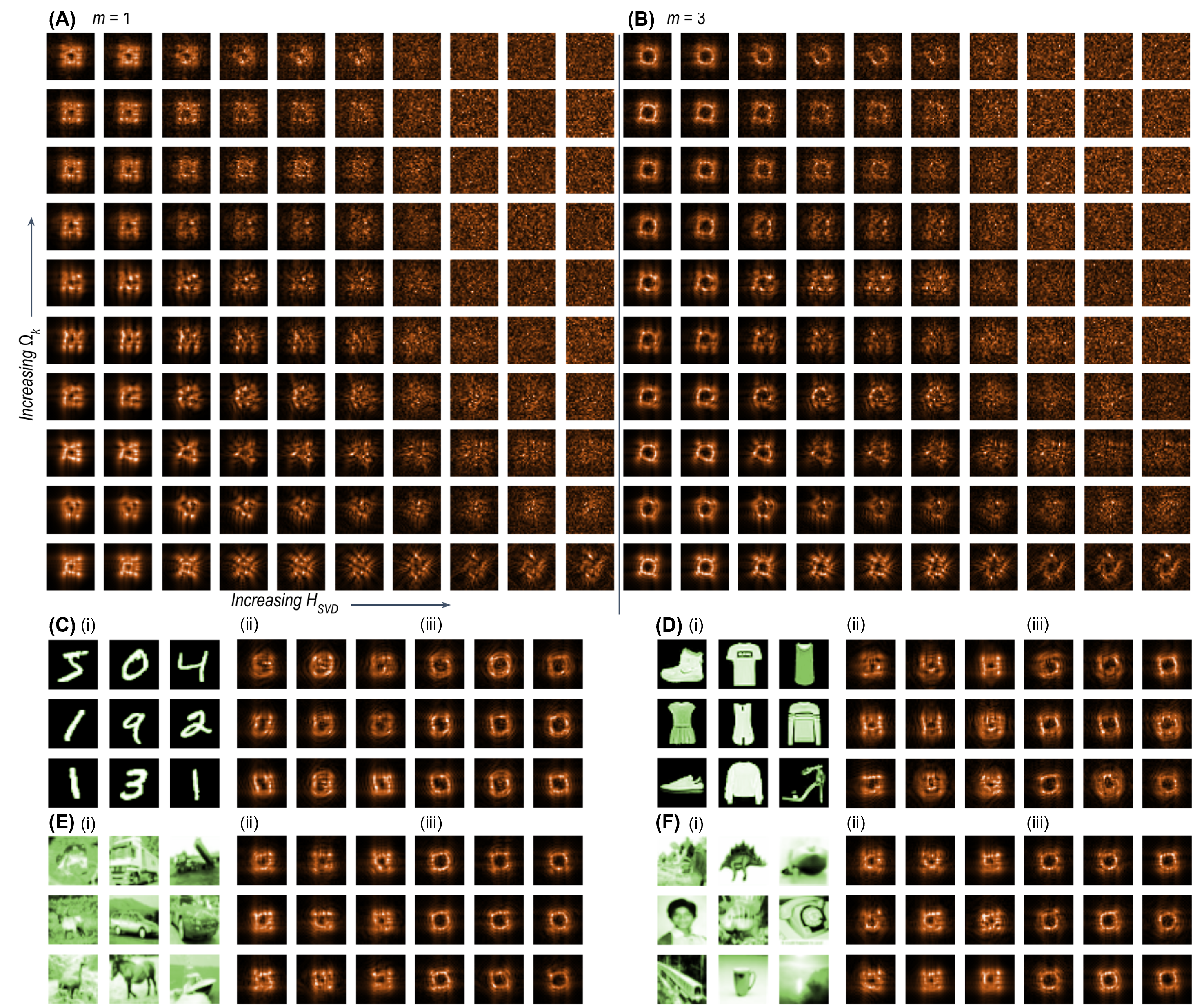
Figure 6: Representative sensor images of the 100 datasets detailed in Fig. 2(B) with encoder topological charge (A) $m=1$ and (B) $m=3$. Nine ground truth images (i) next to their $m=1$ (ii) and $m=3$ (iii) sensor images for (C) MNIST Digits, (D) MNIST Fashion, (E) CIFAR-10, and (F) CIFAR-100 datasets.

4.3 Extension of Figure 4

Additional single pixel responses akin to Fig. 4(B) are shown in Fig. 7. With the models trained on datasets (whose representative images appear in Fig. 2(A)) we show the responses for a centered and an off-axis single pixel in Fig. 8.

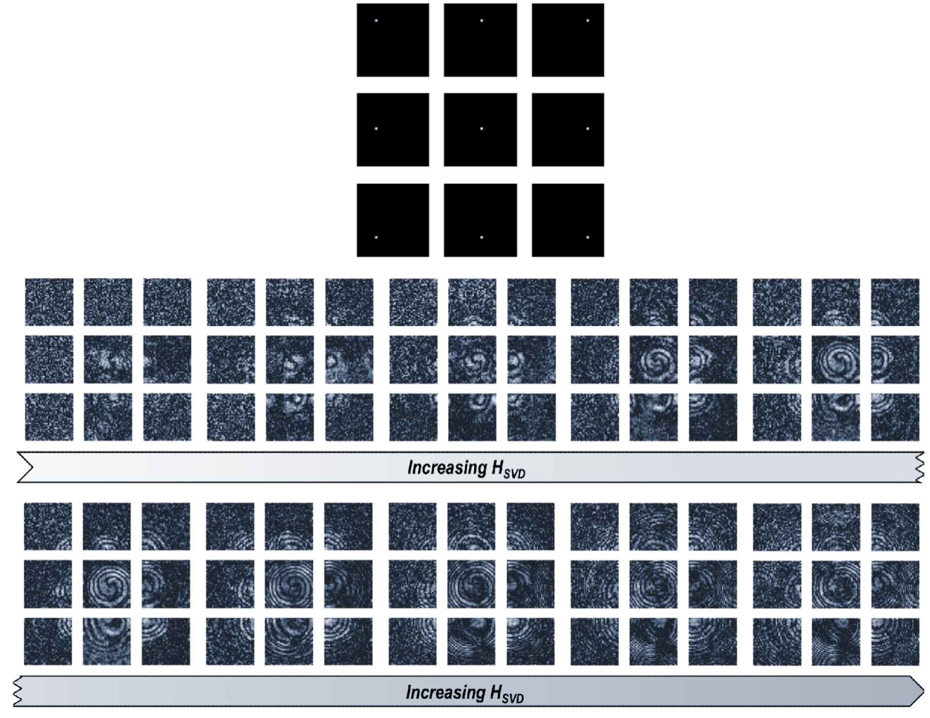
Figure 7: Single pixel response of nine input locations (top) from models trained using the diagonal datasets of Fig. 2(B). This is an extension of Fig. 4 (B).

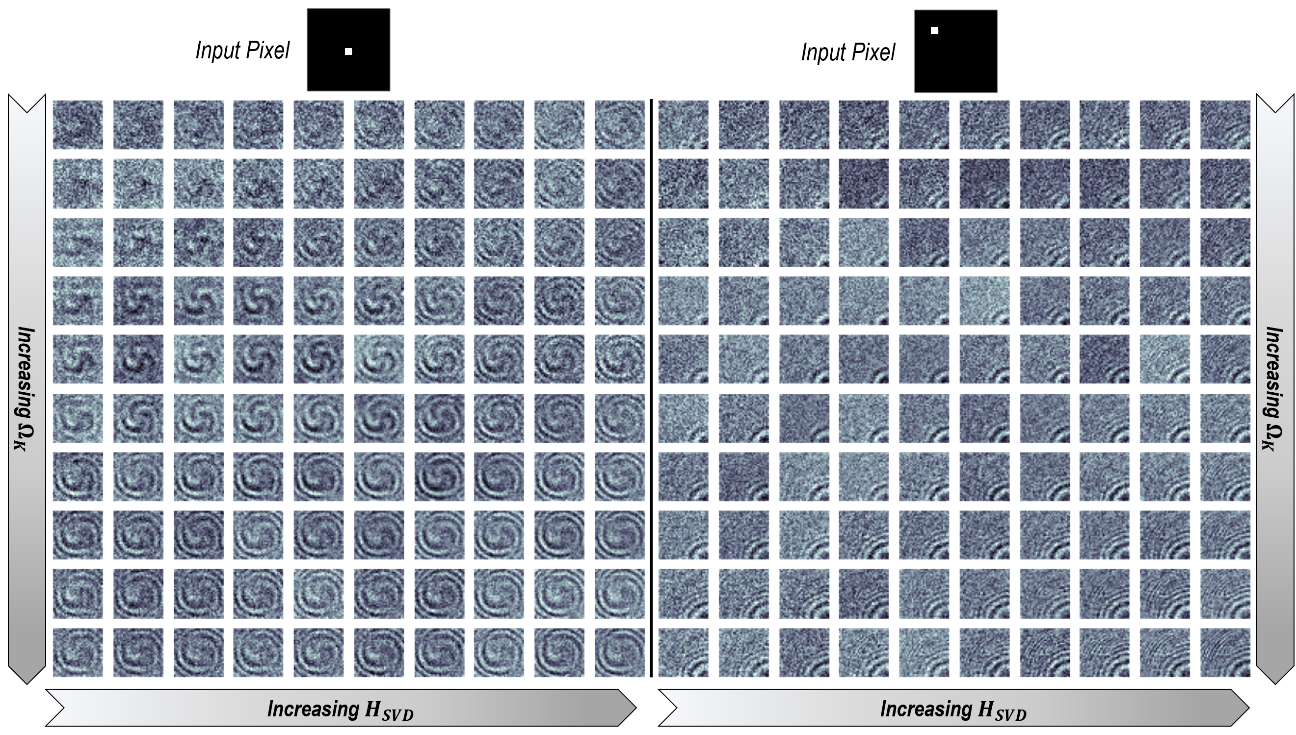
Figure 8: Single pixel response (SPR) of the 100 speckle data sets. Plotted to highlight the change in SPR with both increasing $\Omega_{k}$ and $H_{SVD}$. (left) the SPR of a centered pixel. The most detailed central SPRs are at relatively moderate $H_{SVD}$ and $\Omega_{k}$. (right) The single pixel response of an upper right pixel where the best resolved responses are at high $H_{SVD}$ and high $\Omega_{k}$.

4.4 Extension to Figure 5

Figure 9 shows a more detailed pipeline and classification results from CIFAR-100, as well as CIFAR-10, MNIST Fashion, and MNIST Numbers.

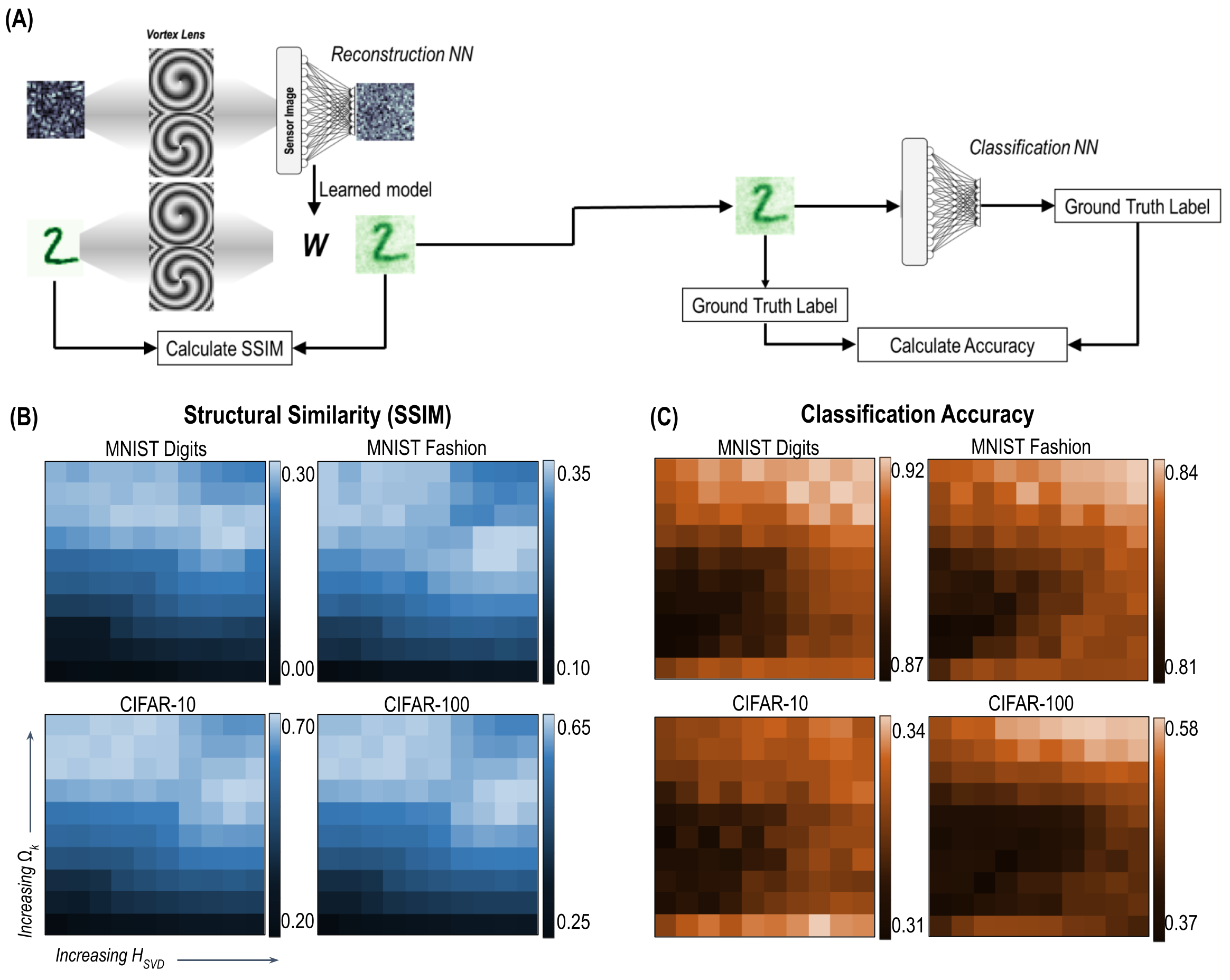
Figure 9: (A) Detailed schematic of the hybrid-optical preprocessed system for classification. A model is trained to reconstruct a particular generalized speckle dataset. That learned model is then used to reconstruct test images (MNIST Digits, MNIST Fashion, CIFAR-10, and CIFAR-100). These reconstructed images are then used to train 2-layer classification NNs. (B) Average Structural Similarity Index (SSIM) of reconstructed test images. Each square corresponds to the SSIM of the particular dataset reconstructed using a model trained with a different dataset. Representative images of the datasets used are shown in a grid with the same orientation in Fig. 1(B). (C) Classification accuracies of a 2-layer NN trained on images reconstructed and represented in (B). Models that were trained on the ground truth images themselves rather than the reconstructed images achieved 94% - MNIST Digits, 86% - MNIST - Fashion, 26% - CIFAR-10, 8.2% - CIFAR-100.

5 Acknowledgements

A.P., X.W., and L.T.V. acknowledge funding from DARPA YFA D19AP00036.

6 Disclosures

The authors declare no conflicts of interest.

References

- [1] L. N. Trefethen, Spectral Methods in MATLAB (Society for Industrial and Applied Mathematics, 2000).
- [2] M. Feit, J. Fleck, and A. Steiger, “Solution of the schrödinger equation by a spectral method,” \JournalTitleJournal of Computational Physics 47, 412–433 (1982).
- [3] A. Weiße, G. Wellein, A. Alvermann, and H. Fehske, “The kernel polynomial method,” \JournalTitleReviews of Modern Physics 78, 275–306 (2006).
- [4] K. J. Burns, G. M. Vasil, J. S. Oishi, D. Lecoanet, and B. P. Brown, “Dedalus: A flexible framework for numerical simulations with spectral methods,” \JournalTitlePhysical Review Research 2 (2020).
- [5] P. Y. Lu, S. Kim, and M. Soljačić, “Extracting interpretable physical parameters from spatiotemporal systems using unsupervised learning,” \JournalTitlePhysical Review X 10 (2020).
- [6] G. Carleo, I. Cirac, K. Cranmer, L. Daudet, M. Schuld, N. Tishby, L. Vogt-Maranto, and L. Zdeborová, “Machine learning and the physical sciences,” \JournalTitleReviews of Modern Physics 91 (2019).
- [7] J. Goodman, Introduction to Fourier Optics, McGraw-Hill physical and quantum electronics series (W. H. Freeman, 2005).
- [8] E. J. Candès, X. Li, and M. Soltanolkotabi, “Phase retrieval from coded diffraction patterns,” \JournalTitleApplied and Computational Harmonic Analysis 39, 277–299 (2015).
- [9] J. Soltau, M. Osterhoff, and T. Salditt, “Coherent diffractive imaging with diffractive optics,” \JournalTitlePhysical Review Letters 128 (2022).
- [10] G. J. Williams, H. M. Quiney, B. B. Dhal, C. Q. Tran, K. A. Nugent, A. G. Peele, D. Paterson, and M. D. de Jonge, “Fresnel coherent diffractive imaging,” \JournalTitlePhysical Review Letters 97 (2006).
- [11] S. Jutamulia, H. Fujii, and T. Asakura, “Double correlation technique for pattern recognition and counting,” \JournalTitleOptics Communications 43, 7–11 (1982).
- [12] G. Wetzstein, A. Ozcan, S. Gigan, S. Fan, D. Englund, M. Soljačić, C. Denz, D. A. B. Miller, and D. Psaltis, “Inference in artificial intelligence with deep optics and photonics,” \JournalTitleNature 588, 39–47 (2020).
- [13] T. Wang, S.-Y. Ma, L. G. Wright, T. Onodera, B. C. Richard, and P. L. McMahon, “An optical neural network using less than 1 photon per multiplication,” \JournalTitleNature Communications 13 (2022).
- [14] B. Muminov and L. T. Vuong, “Fourier optical preprocessing in lieu of deep learning,” \JournalTitleOptica 7, 1079 (2020).
- [15] B. Muminov, A. Perry, R. Hyder, M. S. Asif, and L. T. Vuong, “Toward simple, generalizable neural networks with universal training for low-SWaP hybrid vision,” \JournalTitlePhotonics Research 9, B253 (2021).
- [16] J. Chang, V. Sitzmann, X. Dun, W. Heidrich, and G. Wetzstein, “Hybrid optical-electronic convolutional neural networks with optimized diffractive optics for image classification,” \JournalTitleScientific Reports 8 (2018).
- [17] J. Spall, X. Guo, and A. I. Lvovsky, “Hybrid training of optical neural networks,” \JournalTitleOptica 9, 803 (2022).
- [18] M. Miscuglio, Z. Hu, S. Li, J. K. George, R. Capanna, H. Dalir, P. M. Bardet, P. Gupta, and V. J. Sorger, “Massively parallel amplitude-only fourier neural network,” \JournalTitleOptica 7, 1812 (2020).
- [19] V. Aslani, F. Guerra, A. Steinitz, P. Wilhelm, and T. Haist, “Averaging approaches for highly accurate image-based edge localization,” \JournalTitleOptics Continuum 1, 834 (2022).
- [20] M. Zheng, L. Shi, and J. Zi, “Optimize performance of a diffractive neural network by controlling the fresnel number,” \JournalTitlePhotonics Research 10, 2667 (2022).
- [21] M. Honari-Latifpour, M. S. Mills, and M.-A. Miri, “Combinatorial optimization with photonics-inspired clock models,” \JournalTitleCommunications Physics 5 (2022).
- [22] T. Zhu, C. Guo, J. Huang, H. Wang, M. Orenstein, Z. Ruan, and S. Fan, “Topological optical differentiator,” \JournalTitleNature Communications 12 (2021).
- [23] T. Wang, M. M. Sohoni, L. G. Wright, M. M. Stein, S.-Y. Ma, T. Onodera, M. G. Anderson, and P. L. McMahon, “Image sensing with multilayer nonlinear optical neural networks,” \JournalTitleNature Photonics (2023).
- [24] M. Deng, S. Li, Z. Zhang, I. Kang, N. X. Fang, and G. Barbastathis, “On the interplay between physical and content priors in deep learning for computational imaging,” \JournalTitleOptics Express 28, 24152 (2020).
- [25] N. Antipa, G. Kuo, R. Heckel, B. Mildenhall, E. Bostan, R. Ng, and L. Waller, “Diffusercam: lensless single-exposure 3d imaging,” \JournalTitleOptica 5, 1–9 (2018).
- [26] L. Tian and L. Waller, “3d intensity and phase imaging from light field measurements in an led array microscope,” \JournalTitleOptica 2, 104–111 (2015).
- [27] M. S. Asif, A. Ayremlou, A. Sankaranarayanan, A. Veeraraghavan, and R. Baraniuk, “Flatcam: Thin, bare-sensor cameras using coded aperture and computation,” (2015).
- [28] V. Sitzmann, S. Diamond, Y. Peng, X. Dun, S. Boyd, W. Heidrich, F. Heide, and G. Wetzstein, “End-to-end optimization of optics and image processing for achromatic extended depth of field and super-resolution imaging,” \JournalTitleACM Transactions on Graphics 37, 1–13 (2018).
- [29] L. Valzania and S. Gigan, “Online learning of the transmission matrix of dynamic scattering media,” \JournalTitleOptica 10, 708 (2023).
- [30] V. Klema and A. Laub, “The singular value decomposition: Its computation and some applications,” \JournalTitleIEEE Transactions on Automatic Control 25, 164–176 (1980).
- [31] S. L. Brunton and J. N. Kutz, Data-Driven Science and Engineering: Machine Learning, Dynamical Systems, and Control (Cambridge University Press, USA, 2019), 1st ed.
- [32] Y. Wang and Z. Xu, “Generalized phase retrieval: Measurement number, matrix recovery and beyond,” \JournalTitleApplied and Computational Harmonic Analysis 47, 423–446 (2019).
- [33] S. Aime, M. Sabato, L. Xiao, and D. Weitz, “Dynamic speckle holography,” \JournalTitlePhysical Review Letters 127 (2021).
- [34] L. Devaud, B. Rauer, J. Melchard, M. Kühmayer, S. Rotter, and S. Gigan, “Speckle engineering through singular value decomposition of the transmission matrix,” \JournalTitlePhysical Review Letters 127 (2021).
- [35] J. W. Goodman, “Some fundamental properties of speckle,” \JournalTitleJournal of the Optical Society of America 66, 1145 (1976).
- [36] Z. Wang, A. Bovik, H. Sheikh, and E. Simoncelli, “Image quality assessment: From error visibility to structural similarity,” \JournalTitleIEEE Transactions on Image Processing 13, 600–612 (2004).
- [37] P. N. Belhumeur, J. P. Hespanha, and D. J. Kriegman, “Eigenfaces vs. fisherfaces: recognition using class specific linear projection,” \JournalTitleIEEE Trans. Pattern Anal. Mach. Intell. 19, 711–720 (1997).
- [38] L. T. Vuong, “Compressed sensing and shape extraction with vortex singularities,” in OSA Imaging and Applied Optics Congress 2021 (3D, COSI, DH, ISA, pcAOP), (Optica Publishing Group, 2021).
- [39] I. J. Goodfellow, Y. Bengio, and A. Courville, Deep Learning (MIT Press, Cambridge, MA, USA, 2016). http://www.deeplearningbook.org.
- [40] M. Emschwiller, D. Gamarnik, E. C. Kızıldağ, and I. Zadik, “Neural networks and polynomial regression. demystifying the overparametrization phenomena,” (2020).
- [41] X. Cheng, B. Khomtchouk, N. Matloff, and P. Mohanty, “Polynomial regression as an alternative to neural nets,” (2018).
- [42] O. Alter, P. O. Brown, and D. Botstein, “Singular value decomposition for genome-wide expression data processing and modeling,” \JournalTitleProceedings of the National Academy of Sciences 97, 10101–10106 (2000).
- [43] X. Weng, A. Perry, M. Maroun, and L. T. Vuong, “Singular value decomposition and entropy dimension of fractals,” in 2022 International Conference on Image Processing, Computer Vision and Machine Learning (ICICML), (IEEE, 2022).
- [44] A. Lapidoth, S. M. Moser, and M. A. Wigger, “On the capacity of free-space optical intensity channels,” \JournalTitleIEEE Transactions on Information Theory 55, 4449–4461 (2009).
- [45] Q. Razlighi and N. Kehtarnavaz, “A comparison study of image spatial entropy,” in Visual Communications and Image Processing 2009, vol. 7257 (International Society for Optics and Photonics, 2009), p. 72571X.
- [46] A. Perry, X. Weng, B. Muminov, and L. T. Vuong, “SVD entropy indicates coded diffraction generalized reconstruction accuracy,” in Imaging and Applied Optics Congress 2022 (3D, AOA, COSI, ISA, pcAOP), (Optica Publishing Group, 2022).
- [47] J. Buisine, A. Bigand, R. Synave, S. Delepoulle, and C. Renaud, “Stopping criterion during rendering of computer-generated images based on SVD-entropy,” \JournalTitleEntropy 23, 75 (2021).
- [48] D. A. B. Miller, “Waves, modes, communications, and optics: a tutorial,” \JournalTitleAdv. Opt. Photon. 11, 679–825 (2019).
- [49] J. W. Goodman, Speckle Phenomena in Optics: Theory and Applications, Second Edition (SPIE, 2020).
- [50] M. D. Zeiler and R. Fergus, “Stochastic pooling for regularization of deep convolutional neural networks,” (2013).
- [51] G. Hinton, O. Vinyals, and J. Dean, “Distilling the knowledge in a neural network,” (2015).
- [52] H. Shioya and K. Gohara, “Generalized phase retrieval algorithm based on information measures,” \JournalTitleOptics Communications 266, 88–93 (2006).
- [53] A. Krizhevsky, “Learning multiple layers of features from tiny images,” Tech. rep., University of Toronto (2009).
- [54] V. Antun, F. Renna, C. Poon, B. Adcock, and A. C. Hansen, “On instabilities of deep learning in image reconstruction and the potential costs of AI,” \JournalTitleProceedings of the National Academy of Sciences p. 201907377 (2020).
- [55] S. Ainsworth, “The educational value of multiple-representations when learning complex scientific concepts,” in Visualization: Theory and practice in science education, (Springer, 2008), pp. 191–208.
- [56] G. Mulder, “The concept and measurement of mental effort,” in Energetics and Human Information Processing, (Springer Netherlands, 1986), pp. 175–198.