Preconditioner Design via the Bregman Divergence

Abstract

We study a preconditioner for a Hermitian positive definite linear system, which is obtained as the solution of a matrix nearness problem based on the Bregman log determinant divergence. The preconditioner is of the form of a Hermitian positive definite matrix plus a low-rank matrix. For this choice of structure, the generalised eigenvalues of the preconditioned matrix are easily calculated, and we show under which conditions the preconditioner minimises the $\ell_{2}$ condition number of the preconditioned matrix. We develop practical numerical approximations of the preconditioner based on the randomised singular value decomposition (SVD) and the Nyström approximation and provide corresponding approximation results. Furthermore, we prove that the Nyström approximation is in fact also a matrix approximation in a range-restricted Bregman divergence and establish several connections between this divergence and matrix nearness problems in different measures. Numerical examples are provided to support the theoretical results.

1 Introduction

We study preconditioning of a Hermitian matrix $S=A+B\in\mathbb{C}^{n\times n}$, where $A=QQ^{*}\in\mathbb{C}^{n\times n}$ is positive definite and $B\in\mathbb{C}^{n\times n}$ is Hermitian positive semidefinite. The factor $Q\in\mathbb{C}^{n\times n}$ does not need to be a Cholesky factor and can be a symmetric square root, for instance. Finding $x\in\mathbb{C}^{n}$ such that

$$Sx=b,$$ (1)

encapsulates regularised least squares, Gaussian process regression [31] and is a ubiquitous problem in scientific computing [42, 4]. It also appears in Schur complements of saddle-point formulations of variational data assimilation problems [19, 18]. It is often the case in large-scale numerical linear algebra that interaction with a matrix is only feasible through its action on vectors. Iterative methods such as the conjugate gradient method are therefore of interest for which preconditioning is often a necessity for an efficient and accurate solution, leading to the so-called preconditioned conjugate gradient method (PCG). In this paper, we investigate preconditioners for (1) based on low-rank approximations of the positive semidefinite term of $S$. We can write $S$ as

$$S=Q(I+G)Q^{*},$$

where $G=Q^{-1}BQ^{-*}$. Based on this decomposition we study the two following preconditioners

$$\tilde{S}_{r}=A+B_{r},$$ (2a)

$$\widehat{S}_{r}=Q(I+G_{r})Q^{*},$$ (2b)

where $B_{r}$ and $G_{r}$ are both obtained as truncated SVDs of $B$ and $G$, respectively, where $r<\operatorname{rank}(B)$. While (2a) may seem natural, we show that our proposed preconditioner (2b) is always an improvement and has many useful properties from a practical and theoretical point of view. We also demonstrate that it appears naturally as the minimiser of a matrix nearness problem in the Bregman divergence. This is intuitive since it is desirable to seek a preconditioner that is, in some sense, close to the matrix $S$.

Our main contribution is the development of a general framework for the design of preconditioners for (1) based on the Bregman log determinant divergence. First, Section 2 examines the two preconditioners in (2) more closely based on straightforward eigenvalue analysis and presents a simple example to develop intuition. We then introduce the Bregman divergence framework in Section 3. We prove that our proposed preconditioner (2b) minimises the Bregman divergence to the original matrix $S$ in Theorem 1 (and in some cases, the condition number of the preconditioned matrix), and demonstrate how it can improve the convergence of PCG in Section 3.3. In Section 4, we make a connection between different norm minimisation problems and the Bregman divergence framework. We also derive the Nyström approximation in several different ways, one of which is as a minimiser of a range-restricted Bregman divergence. Next, Section 5 explores practical numerical methods based on randomised linear algebra for the approximations of our preconditioner in the big data regime where the truncated SVD becomes computationally intractable. Section 6 supports our theoretical findings with numerical experiments for equation (1) using various preconditioners. Section 7 contains a summary.

1.1 Related Work

Preconditioning and matrix approximation are closely linked since a preconditioner $\mathcal{P}$ is typically chosen such that, in some sense, $\mathcal{P}\approx S$, subject to the requirement that $\mathcal{P}$ respects some computational budget in terms of storage, action on vectors, and its factorisation. In this paper, we establish a natural connection between matrix nearness problems in the Bregman divergence and preconditioning. The use of divergences in linear algebra is not novel. [10] proposed the use of the Bregman divergences for matrix approximation problems motivated by their connection to exponential families of distributions. Also relevant to our work is [27] where the authors investigate extensions of divergences to the low-rank matrices in the context of kernel learning. We build on these ideas in Section 4 and show the connection between the Bregman divergence and the Nyström approximation. The latter is becoming increasingly popular in numerical linear algebra, in particular in the context of randomised matrix approximation methods. Many such methods are based on sketching [41], a technique whereby a matrix $A\in\mathbb{C}^{n\times n}$ is multiplied by some sketching matrix $\Omega\in\mathbb{R}^{n\times r}$, $r<n$ producing a compressed matrix $A\Omega$ which is used to compute approximations of $A$. As mentioned, randomised methods select $\Omega$ as a random matrix providing the setting for probabilistic bounds on the accuracy of the approximation, see [29, 24]. Methods such as the randomised SVD and the Nyström approximation offer practical alternatives to the truncated SVD with both affordable computational cost and certain theoretical guarantees. Such approximations have long been popular in the kernel-based learning community [40, 11]. Preconditioning is becoming more relevant for the data science and machine learning communities with the increasing demand for handling large-scale problems. Recently, the work of [17] introduced a Nyström-based preconditioner for PCG for matrices $\mu I+A$ for some scalar $\mu>0$, where $A$ is symmetric positive semidefinite. This strategy has also been applied to the alternating method of multipliers [43], and sketching more generally to a stochastic quasi-Newton method in [16]. Applications such as large-scale Gaussian process regression can also benefit from the development of the preconditioners introduced in this work since gradient-based parameter optimisation requires expensive linear solves for optimising kernel hyperparameters [38].

1.2 Notation & Preliminaries

Definition 1.

Let $\mathbb{H}^{n}$ denote the space of Hermitian $n\times n$ matrices. ${\mathbb{H}^{n}_{+}}\subset\mathbb{H}^{n}$ denotes the cone of positive semidefinite matrices and ${\mathbb{H}^{n}_{++}}=\operatorname{int}{\mathbb{H}^{n}_{+}}$ the positive definite cone.

Definition 2.

Let $\lambda(A)=\{\lambda_{1}(A),\ldots,\lambda_{n}(A)\}$, with $\lambda_{1}(A)\geq\ldots\geq\lambda_{n}(A)$, denote the ordered eigenvalues of a matrix $A\in\mathbb{C}^{n\times n}$ Further, let $\sigma(A)=\{\sigma_{1}(A),\ldots,\sigma_{n}(A)\}$ denote the similarly ordered singular values of a matrix $A\in\mathbb{C}^{n\times n}$. For nonsingular normal matrices $A$ we denote the $\ell_{2}$ condition number by $\kappa_{2}(A)=\frac{\sigma_{1}(A)}{\sigma_{n}(A)}$.

We denote by $A:B:=\operatorname{trace}\big{(}A^{*}B\big{)}$ the trace inner product between two matrices $A$ and $B$. $I$ denotes the identity matrix, sometimes with a subscript to denote the dimension if it is not clear from the context. $\|\cdot\|_{F}$ denotes the Frobenius norm and $\|\cdot\|_{2}$ the $\ell_{2}$ norm. $A^{+}$ denotes the Moore-Penrose inverse of $A$. $A_{r}$ will in general be used to denote a rank $r$ approximation of $A$ obtained via a truncated SVD. When $A$ is positive definite we define the induced norm $\|\cdot\|_{A}$ by the relation

$$\|x\|_{A}^{2}=x^{*}Ax.$$

Convex analysis is a natural tool for studying the Bregman divergence, so we recall some elementary definitions, see [32] for more details. We restrict our attention to spaces of finite dimension. The relative interior, $\operatorname{ri}C$, of a convex set $C$ is the subset of $C$ which can be considered as an affine subset of $C$, i.e.,

$$\operatorname{ri}C=\{x\in C\,|\,\exists\;\textnormal{neighbourhood}\;V\textnormal{of}\;x\;\textnormal{such that}\;V\cap\operatorname{aff}C\subseteq C\},$$

where $\operatorname{aff}C$ is the affine hull of $C$. Let $\mathcal{X}$ be some finite-dimensional real inner product space. The effective domain of a function $\phi:\mathcal{X}\rightarrow\mathbb{R}\cup\{-\infty,+\infty\}$ is defined by

$$\operatorname{dom}\phi=\{x\in\mathcal{X}\,|\,\phi(x)<\infty\}.$$

A convex function $\phi$ is proper if it never attains the value $-\infty$ and that there exists a point $x\in\mathcal{X}$ for which $\phi(x)$ is finite.

2 Spectral and Other Properties

In this section, we develop some intuition about the two preconditioners $\tilde{S}_{r}$ and $\widehat{S}_{r}$ defined in (2) by straightforward analysis of the eigenvalues of the preconditioned matrices $\tilde{S}_{r}^{-1}S$ and $\widehat{S}_{r}^{-1}S$. Their respective inverses are given by

$$\tilde{S}_{r}^{-1} =Q^{-*}(I+Q^{-1}B_{r}Q^{-*})^{-1}Q^{-1},$$

$$\widehat{S}_{r}^{-1} =Q^{-*}(I+G_{r})^{-1}Q^{-1}.$$

Lemma 1.

The eigenvalues of $\tilde{S}_{r}^{-1}S$ and $\widehat{S}_{r}^{-1}S$ satisfy the following bounds for $i=1,\ldots,n$:

$$\lambda_{i}(\tilde{S}_{r}^{-1}S)\in\left[1,1+\lambda_{1}(G)\right],$$

$$\lambda_{i}(\widehat{S}_{r}^{-1}S)\in\left[1,1+\lambda_{r+1}(G)\right].$$

Proof.

Recall that $B_{r}$ and $G_{r}$ are obtained as truncated SVDs of $B$ and $G$, respectively, where $r<\operatorname{rank}(B)$. We obtain the result by observing the following bounds for the Rayleigh quotients below, where $x\in\mathbb{C}^{n}$ and not identically zero:

$$\frac{x^{*}(I+G)x}{x^{*}(I+Q^{-1}B_{r}Q^{-*})x} \in\left[1,1+\lambda_{1}(G)\right],$$ (3a)

$$\frac{x^{*}(I+G)x}{x^{*}(I+G_{r})x} \in\left[1,1+\lambda_{r+1}(G)\right].$$ (3b)

∎

The bound (3a) is of course pessimistic, but it is in general difficult to infer a tighter upper bound here since $G$ and $Q^{-1}B_{r}Q^{-*}$ are not a priori simultaneously diagonalisable. Later, in Theorem 2, we show that when $G$ does not have full rank (but not necessarily low rank), $\widehat{S}_{r}$ minimises the conditioner number of the preconditioned matrix among matrices of the form $A+W$, where $W\in{\mathbb{H}^{n}_{+}}$ has at rank at most $r$. We defer a more detailed analysis to Section 3, but this result motivates the study of (2).

Next we present a simple example illustrating the difference between $\widehat{S}_{r}$ and $\tilde{S}_{r}$. Let $A$ and $B$ be diagonal $6\times 6$ matrices:

$$A=\operatorname{diag}(1.1,1.05,0.375,0.05,0.05,0.05),\qquad B=\operatorname{diag}(1,0.5,0.25,0.1,0,0).$$ (4)

This results in

$$G=\operatorname{diag}(\mathbf{0.9091},0.4762,0.6667,\mathbf{2},0,0),$$ (5a)

$$Q=\operatorname{diag}(1.0488,1.0247,0.6124,0.2236,0.2236,0.2236),$$ (5b)

where, for ease of exposition, we truncate after the fourth decimal. We observe $\operatorname{rank}(B)=4$, and take $r=2$ in the low-rank approximations of the positive semidefinite term. A truncated SVD will pick out the indices corresponding to the $r$ largest numbers (in bold). On the other hand, we find that

$$Q^{-1}B_{r}Q^{-*}=\operatorname{diag}(\mathbf{0.9091},\mathbf{0.4762},0,0,0,0).$$

The resulting generalised eigenvalues are shown in Figure 1.

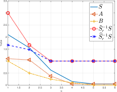
Figure 1: Eigenvalues of $S$ and generalised eigenvalues of the preconditioned system using the preconditioners $\tilde{S}_{r}$ and $\widehat{S}_{r}$.

Recall that

$$\tilde{S}_{r}^{-1}S =Q^{-*}(I+Q^{-1}B_{r}Q^{-*})^{-1}(I+G)Q^{*},$$

$$\widehat{S}_{r}^{-1}S =Q^{-*}(I+G_{r})^{-1}(I+G)Q^{*}.$$

For the instances of $A$ and $B$ in (4) we therefore have, by direct calculation,

$$\lambda_{i}(Q^{-1}B_{r}Q^{-*})=\lambda_{i}(B)\lambda_{i}(A)^{-1},\quad i=1,\ldots,r,$$

and

$$\lambda_{1}(G_{r})=B_{44}A_{44}^{-1},\quad\lambda_{2}(G_{r})=\lambda_{1}(B)\lambda_{1}(A)^{-1},$$

which clearly shows the scaling effect. In particular, we note that

$$\lambda_{2}(G_{r})=\lambda_{1}(Q^{-1}B_{r}Q^{-*}).$$

There is no difference when the spectrum of $A$ is flat, but if the spectrum of $A$ decays as above, then $\lambda_{i}(Q^{-1}B_{r}Q^{-*})$ will be dominated by $\lambda_{i}(G_{r})$ in which case:

$$1\leq\lambda_{i}(\widehat{S}_{r}^{-1}S)<\lambda_{i}(\tilde{S}_{r}^{-1}S),\qquad i=1,\ldots,n.$$

We highlight a situation where $\widehat{S}_{r}=\tilde{S}_{r}$. Suppose that we had defined $B$ by reversing the order of the non-zero diagonal elements in (4), i.e.,

$$B^{\textnormal{rev}}=\operatorname{diag}(0.1,0.25,0.5,1,0,0).$$

In this case,

$$G^{\textnormal{rev}}=\operatorname{diag}(1.1^{-1},0.2381,\mathbf{1.3333},\mathbf{20},0,0),$$ (6)

and

$$Q^{-1}B_{r}^{\textnormal{rev}}Q^{-1}=\operatorname{diag}(0,0,\mathbf{1.3333},\mathbf{20},0,0)=G_{r}^{\textnormal{rev}}.$$

By comparing (5a) and (6), we notice the largest eigenvalues (in bold) have different indices, representing the loss of information when prematurely truncating $B$ before scaling by the factors of $A^{-1}$. This suggests that this scaling can, in some circumstances, improve the approximation of $S$. While this approach uses $G$ explicitly, we show in Section 5 economical ways of computing with it using only matrix-vector products. In the general case where the basis is not given by the identity, analysis of the generalised eigenvalues is of course insufficient to determine the quality of the associated preconditioners, a point to which we return later.

Corollary 1.

$\widehat{S}_{r}=\tilde{S}_{r}$ when $A$ is a scaled identity.

Proof.

Let $A=\alpha I$ for some $\alpha>0$. Then,

$$G_{r}=(\alpha^{-1/2}B\alpha^{-1/2})_{r}=\alpha^{-1}B_{r}=Q^{-1}B_{r}Q^{-*}.$$

∎

3 Preconditioners via Bregman Projections

In this section we analyse the problem of finding a preconditioner by using the Bregman divergence. We will formulate this as a constrained optimisation problem and prove (2b) is a minimiser. We also present a result concerning the optimality of the condition number of the resulting preconditioned matrix. Section 3.1 discusses extentions of this framework, and in Section 3.2 we give an example of how certain diagonal preconditioners can be derived from the proposed framework. Finally, Section 3.3 summarises the consequences of our theoretical results in the context of PCG.

It is well-known that a truncated singular value decomposition is an optimal low-rank approximation in both the spectral and Frobenius norms thanks to the Eckart–Young–Mirsky theorem. These norms are not invariant under congruence transformations, i.e., $Z\mapsto P^{*}ZP$ for some invertible $P$, and we will discover in Section 4 that the preconditioners $\tilde{S}_{r}$ and $\widehat{S}_{r}$ are optimal solutions to different matrix norm minimisation problems. In this section, we introduce a different nearness measure, the Bregman divergence, which naturally leads to the preconditioner $\widehat{S}_{r}$.

The Bregman matrix divergence $\mathcal{D}_{\phi}:\operatorname{dom}\phi\times\operatorname{ri}\operatorname{dom}\phi\rightarrow[0,\infty)$ associated with a proper, continuously-differentiable, strictly convex seed function $\phi$ is defined as follows:

$$\mathcal{D}_{\phi}(X,Y) =\phi(X)-\phi(Y)-\operatorname{trace}\big{(}\nabla\phi(Y)^{*}(X-Y)\big{)}.$$

This divergence originated in convex analysis for finding intersections of convex sets [5], and divergences are now central objects in the field of information geometry, see e.g. [1, 2]. The choices $\phi(X)=\operatorname{trace}\big{(}X\log X-X\big{)}$, $\phi(X)=\|X\|_{F}^{2}$ and $\phi(X)=-\log\det(X)$ lead to the von Neumann, squared Frobenius and log determinant (or Burg) divergences, respectively, where $\log$ in this context is the matrix logarithm:

$$\mathcal{D}_{\textnormal{VN}}(X,Y)=\operatorname{trace}\big{(}X\log X-X\log Y-X+Y\big{)},\qquad \operatorname{dom}\phi={\mathbb{H}^{n}_{++}},$$

$$\mathcal{D}_{\textnormal{F}}(X,Y)=\|X-Y\|_{F}^{2}, \operatorname{dom}\phi=\mathbb{H}^{n},$$

$$\mathcal{D}_{\textnormal{LD}}(X,Y)=\operatorname{trace}\big{(}XY^{-1}\big{)}-\log\det(XY^{-1})-n, \operatorname{dom}\phi={\mathbb{H}^{n}_{++}}.$$

By a limit argument [27, Section 4], the log determinant matrix divergence is only finite if $\operatorname{range}X=\operatorname{range}Y$, or $\operatorname{range}X\subseteq\operatorname{range}Y$ for the von Neumann divergence. We highlight a few useful properties of the divergences, collectively denoted by $\mathcal{D}_{\phi}$ [10]:

• $\mathcal{D}_{\phi}(X,Y)=0\Leftrightarrow X=Y$,

• Nonnegativity: $\mathcal{D}_{\phi}(X,Y)\geq 0$,

• Convexity: $X\rightarrow\mathcal{D}_{\phi}(X,Y)$ is convex.

We also state the following facts about these divergences:

Corollary 2 ([27, Corollary 2]).

Given eigendecompositions

$$X=U\operatorname{diag}(\lambda)U^{*},$$

$$Y=V\operatorname{diag}(\theta)V^{*},$$

with unitary $U$ and $V$ whose columns consist of eigenvectors $u_{i}$ and $v_{i}$, respectively, the squared Frobenius, von Neumann and log determinant matrix divergences satisfy:

$$\mathcal{D}_{\textnormal{LD}}(X,Y)=\sum_{i=1}^{n}\sum_{j=1}^{n}(v_{i}^{*}u_{j})^{2}\left[\frac{\lambda_{i}}{\theta_{j}}-\log\frac{\lambda_{i}}{\theta_{j}}-1\right],$$ (8a)

$$\mathcal{D}_{\textnormal{VN}}(X,Y)=\sum_{i=1}^{n}\sum_{j=1}^{n}(v_{i}^{*}u_{j})^{2}[\lambda_{i}\log\lambda_{i}-\lambda_{i}\log\theta_{j}-\lambda_{i}+\theta_{j}],$$ (8b)

$$\mathcal{D}_{\textnormal{F}}(X,Y)=\sum_{i=1}^{n}\sum_{j=1}^{n}(v_{i}^{*}u_{j})^{2}[\lambda_{i}-\theta_{j}]^{2}.$$ (8c)

Proposition 1 ([27, Proposition 12]).

Let $P$ be invertible so $Z\mapsto f(Z)=P^{*}ZP$ is a congruence transformation. Then,

$$\mathcal{D}_{\textnormal{LD}}(X,Y)=\mathcal{D}_{\textnormal{LD}}(f(X),f(Y)).$$

From Proposition 1, we have

$$\mathcal{D}_{\textnormal{LD}}(\widehat{S}_{r},S) =\mathcal{D}_{\textnormal{LD}}(Q(I+G_{r})Q^{*},Q(I+Q^{-1}BQ^{-*})Q^{*})$$

$$=\mathcal{D}_{\textnormal{LD}}(I+G_{r},I+Q^{-1}BQ^{-*}).$$ (9)

In light of this, we ask if $G_{r}$ is in fact a solution to the problem

$$\operatorname*{minimise}_{X\in{\mathbb{H}^{n}_{+}}}\quad \mathcal{D}_{\textnormal{LD}}(\mathcal{P},S)$$ (10a)

$$\operatorname*{s.t.}\quad \mathcal{P}=Q(I+X)Q^{*}$$ (10b)

$$\operatorname{rank}(X)\leq r,$$ (10c)

or, equivalently,

$$\operatorname*{minimise}_{X\in{\mathbb{H}^{n}_{+}}}\quad \mathcal{D}_{\textnormal{LD}}(I+X,I+Q^{-1}BQ^{-*})$$

$$\operatorname*{s.t.}\quad \operatorname{rank}(X)\leq r.$$

We answer this question in the affirmative with the following Theorem.

Theorem 1.

$\widehat{S}_{r}$ defined in (2b) is a minimiser of (10). Furthermore, the first $\operatorname{rank}(B)-r$ eigenvalues of $\widehat{S}_{r}^{-1}S$ are given by $1+\lambda_{r+i}(G)$, $i=1,\ldots,\operatorname{rank}(B)-r$, and the remaining ones are given by $1$ with multiplicity $n+r-\operatorname{rank}(B)$.

Proof.

We derive a lower bound for $\mathcal{P}\mapsto\mathcal{D}_{\textnormal{LD}}(\mathcal{P},S)$. Let $\mathcal{P}=V\Sigma V^{*}$, $\Sigma=\operatorname{diag}(\sigma)$ and $S=U\Lambda U^{*}$, $\Lambda=\operatorname{diag}(\lambda)$. The first term of the divergence is $\operatorname{trace}\big{(}\mathcal{P}S^{-1}\big{)}$, which can be written as

$$\operatorname{trace}\big{(}\mathcal{P}S^{-1}\big{)} =\operatorname{trace}\big{(}V\Sigma V^{*}U\Lambda^{-1}U^{*}\big{)}=\operatorname{trace}\big{(}\Sigma P\Lambda^{-1}P^{*}\big{)},$$

where $P=V^{*}U$ is unitary. Since $P\mapsto\operatorname{trace}\big{(}\Sigma P\Lambda^{-1}P^{*}\big{)}$ is a continuous map over a compact set (the orthogonal group), it will attain its extrema in this set by Weierstrass’ theorem. As a result, we obtain the following lower bound [6]:

$$\operatorname{trace}\big{(}\mathcal{P}S^{-1}\big{)}\geq\sum_{i=1}^{n}\sigma_{i}\lambda_{i}^{-1}.$$

Now note that $I+G_{r}$ and $I+Q^{-1}BQ^{-*}$ are simultaneously diagonalisable so they share an eigenbasis with eigenvectors $u_{i}$, $i=1,\ldots n$. Let $1+\nu_{i}$ be the eigenvalues of $I+G_{r}$ and $1+\mu_{i}$ the eigenvalues of $I+Q^{-1}BQ^{-*}$. We have, by construction, $\nu_{i}=\mu_{i}$ for $1\leq i\leq r$, $\nu_{i}=0$ for $r+1\leq i$. Then we have the lower bound on the log determinant term as a function of $\Sigma$, which is realised by the choice $X=G_{r}$ in (10b):

$$-\log\det(\mathcal{P}S^{-1})=-\sum_{i=1}^{n}\log\left(\frac{1+\sigma_{i}}{1+\mu_{i}}\right)\geq-\sum_{i=r+1}^{n}\log\left(\frac{1}{1+\mu_{i}}\right).$$

This implies that for any $\mathcal{P}$, we have

$$\mathcal{D}_{\textnormal{LD}}(\mathcal{P},S)\geq\sum_{i=1}^{n}\sigma_{i}\lambda_{i}^{-1}-\sum_{i=r+1}^{n}\log\left(\frac{1}{1+\mu_{i}}\right)-n.$$ (11)

Using Corollary 2 and orthogonality of the eigenvectors we obtain

$$\mathcal{D}_{\textnormal{LD}}(\widehat{S}_{r},S) =\mathcal{D}_{\textnormal{LD}}(I+G_{r},I+Q^{-1}BQ^{-*})$$

$$=\sum_{i=1}^{n}\sum_{j=1}^{n}(u_{i}^{*}u_{j})^{2}\left(\frac{1+\nu_{i}}{1+\mu_{j}}-\log\left(\frac{1+\nu_{i}}{1+\mu_{j}}\right)-1\right)$$

$$=\sum_{j=r+1}^{\operatorname{rank}(B)}\left(\frac{1}{1+\mu_{j}}-\log\left(\frac{1}{1+\mu_{j}}\right)-1\right).$$ (12)

This coincides with the lower bound (11), so the first result follows. The statement concerning the generalised eigenvalues follows since $G_{r}$ and $G$ are simultaneously diagonalisable by construction. ∎

We can also ask if $G_{r}$ satisfies a similar result. Since the domain of the divergence is ${\mathbb{H}^{n}_{++}}\times{\mathbb{H}^{n}_{++}}$ we cannot say that $G_{r}$ is the matrix such that $\mathcal{D}_{\textnormal{LD}}(G_{r},G)$ is minimised. We can, however, state a different result.

Proposition 2.

Let $VMV^{*}$ be an eigendecomposition of $G=Q^{-1}BQ^{-*}$ and $V_{r}$ the first $r<n$ columns of $V$. The rank $r$ approximation of $G$ obtained by a truncated singular value decomposition, $G_{r}$, is a minimiser of

$${\mathbb{H}^{n}_{+}}\ni X\mapsto\mathcal{D}(V_{r}^{*}XV_{r},V_{r}^{*}GV_{r}),$$

where $X$ is such that $V_{r}^{*}XV_{r}\in{\mathbb{H}^{r}_{++}}$ and $\operatorname{rank}(X)\leq r$ and $\mathcal{D}$ can be either the von Neumann or log determinant divergence.

Proof.

This follows trivially from direct computation. Indeed, $V_{r}^{*}GV_{r}=M_{r}$, where $M_{r}$ is the $\mathbb{R}^{r\times r}$ submatrix of $M$ containing the first $r$ eigenvalues of $G$. So, by construction,

$$\mathcal{D}(V_{r}^{*}G_{r}V_{r},V_{r}^{*}GV_{r}) =\mathcal{D}(V_{r}^{*}V_{r}M_{r}V_{r}^{*}V_{r},V_{r}^{*}VMV^{*}V_{r})$$

$$=\mathcal{D}(M_{r},M_{r})$$

$$=0.$$

Since $0$ is a lower bound of the convex function $X\mapsto\mathcal{D}(V_{r}^{*}XV_{r},V_{r}^{*}GV_{r})$, we are done. ∎

[27] extends the divergences to low-rank matrices, which will be explored in more detail in the context of Nyström approximations in Section 4.

Remark 1.

The quantities $\mathcal{D}_{\textnormal{LD}}(\widehat{S}_{r},S)$ and $\mathcal{D}_{\textnormal{LD}}(\tilde{S}_{r},S)$ are described in terms of the eigenvalues of $I+G$, $I+G_{r}$ and $I+Q^{-1}B_{r}Q^{-*}$. By construction,

$$\lambda_{i}(I+G_{r})=\lambda_{i}(I+G)\quad\textnormal{when}\quad 1\leq i\leq r,$$

so the divergence $\mathcal{D}_{\textnormal{LD}}(\widehat{S}_{r},S)$ in (12) measures a quantity in terms of the $i$th eigenvalues, where $r+1\leq i\leq n$.
An attempt to carry out the same analysis for $\mathcal{D}_{\textnormal{LD}}(\tilde{S}_{r},S)$ makes it clear why we expect $\widehat{S}_{r}$ to be a better preconditioner. The derivation of the bound (12) relies on the fact that $I+G_{r}$ and $I+G$ are simultaneously diagonalisable. In general, however, $Q^{-1}B_{r}Q^{-*}\neq G_{r}$ (see Corollary 1). Letting $(u_{i},1+\mu_{i})$ and $(\tilde{u}_{i},1+\tilde{\nu}_{i})$ denote the eigenpairs of $I+G$ and $I+Q^{-1}B_{r}Q^{-*}$, respectively, we have:

$$\mathcal{D}_{\textnormal{LD}}(\tilde{S}_{r},S)=\sum_{i=1}^{n}\sum_{j=1}^{n}(\tilde{u}_{i}^{*}u_{j})^{2}\left(\frac{1+\tilde{\nu}_{i}}{1+\mu_{j}}-\log\left(\frac{1+\tilde{\nu}_{i}}{1+\mu_{j}}\right)-1\right).$$ (13)

The importance of the choice of basis is also apparent from the term $(\tilde{u}_{i}^{*}u_{j})^{2}$ in (13), since this measures how aligned the bases are between $S$ and its preconditioner. To summarise, a reason for $\widehat{S}_{r}$ appearing to be a better preconditioner is that it matches the eigenvalues of $S$ in the first parts of the spectrum i.e. $[1,r]$, which directly implies unit eigenvalues of the multiplicity mentioned in Theorem 1.

Corollary 3.

$\mathcal{D}_{\textnormal{LD}}(\tilde{S}_{r},S)\geq\mathcal{D}_{\textnormal{LD}}(\widehat{S}_{r},S)$.

While corollary 3 is trivial, its significance in terms of interpreting preconditioning strategies for $S$ is not yet clear. If $D(X,Z)<D(Y,Z)$, then we in general expect the matrix $XZ^{-1}$ to be closer to the identity than $YZ^{-1}$, but the quality of a preconditioner depends not only on the bounds for the eigenvalues but also on the distribution of the spectrum. Based on Remark 1 and Theorem 1, the basis for the preconditioner also plays a part. This is discussed in Section 3.3 in the context of iterative methods. We conclude this section with a result regarding the condition number of the preconditioned matrix:

Theorem 2.

When $\operatorname{rank}(G)<n$, $G_{r}$ is a minimiser of the problem

$$\operatorname*{minimise}_{X\in{\mathbb{H}^{n}_{+}}}\quad \kappa_{2}(P^{-{\frac{1}{2}}}SP^{-{\frac{1}{2}}})$$ (14a)

$$\operatorname*{s.t.}\quad P=Q(I+X)Q^{*}$$ (14b)

$$\operatorname{rank}(X)\leq r.$$ (14c)

Proof.

By definition, we have $\kappa_{2}(P^{-{\frac{1}{2}}}SP^{-{\frac{1}{2}}})=\frac{\lambda_{1}(P^{-{\frac{1}{2}}}SP^{-{\frac{1}{2}}})}{\lambda_{n}(P^{-{\frac{1}{2}}}SP^{-{\frac{1}{2}}})}$. We find a lower bound for $\lambda_{1}({P^{-{\frac{1}{2}}}SP^{-{\frac{1}{2}}}})$ independent of the choice of $X$. First, note that

$$\lambda_{1}({P^{-{\frac{1}{2}}}SP^{-{\frac{1}{2}}}})=\lambda_{1}(P^{-1}S)=\lambda_{1}({(I+Q^{-1}XQ^{-*})^{-1}(I+G))}.$$

Then,

$$\lambda_{1}({(I+Q^{-1}XQ^{-*})^{-1}(I+G))}=\max_{0\neq x\in\mathbb{C}^{n}}\frac{x^{*}(I+G)x}{x^{*}(I+Q^{-1}XQ^{-*})x}\geq 1+\lambda_{r+1}(G).$$

We now provide an upper bound on $\lambda_{n}(P^{-{\frac{1}{2}}}SP^{-{\frac{1}{2}}})$. By definition,

$$\lambda_{n}(P^{-{\frac{1}{2}}}SP^{-{\frac{1}{2}}})=\lambda_{n}((I+Q^{-1}XQ^{-*})^{-1}(I+G)).$$

We assume $\ker(G)\neq\emptyset$, and since $Q^{-1}XQ^{-*}$ is positive semidefinite for any $X\in{\mathbb{H}^{n}_{+}}$ with rank at most $r$, we have

$$\lambda_{n}(P^{-{\frac{1}{2}}}SP^{-{\frac{1}{2}}})\leq 1.$$

Consequently, we have

$$\kappa_{2}(P^{-{\frac{1}{2}}}SP^{-{\frac{1}{2}}})\geq 1+\lambda_{r+1}(G).$$

The choice $X=G_{r}$ in (14b) leads to

$$P=Q(I+G_{r})Q^{*}=\widehat{S}_{r}.$$

We have $\lambda_{1}(\widehat{S}_{r}^{-1}S)=1+\lambda_{r+1}(G)$ thanks to Theorem 1 so we are done. ∎

When $G$ has full rank, Theorem 1 still holds, but Theorem 2 does not apply. To see why, observe that

$$\lambda_{n}(P^{-1}S)=\lambda_{n}((I+Q^{-1}XQ^{-*})^{-1}(I+G))\leq\lambda_{n}(I+G),$$

so the general bound for the preconditioned matrix is

$$\kappa_{2}(P^{-1}S)\leq\frac{1+\lambda_{r+1}(G)}{1+\lambda_{n}(G)}.$$

We have $\lambda_{n}(\widehat{S}_{r}^{-1}S)=1\leq 1+\lambda_{n}(G)$. Therefore, $1+\lambda_{r+1}(G)=\kappa_{2}(\widehat{S}_{r}^{-1}S)\geq\frac{1+\lambda_{r+1}(G)}{1+\lambda_{n}(G)}$. However, we can still construct a preconditioner that minimises the condition number of the preconditioned matrix

$$Q(I+G_{r}+\alpha(I-VV^{*}))Q^{*},$$ (15)

where the columns of $V\in\mathbb{C}^{n\times r}$ are the $r$ left dominant singular vectors of $G_{r}$ and selecting $\lambda_{n}(G)\leq\alpha\leq\lambda_{r+1}(G)$ since it lifts the eigenvalues of $\widehat{S}_{r}^{-1}S$ that are not unity to the interval $[\lambda_{n}(G),\lambda_{r+1}(G)]$. A similar approach is used in [43]. The application of (15) can be applied at similar computational cost to (2b) but assumes knowledge of the interval in which $\alpha$ must be chosen. In addition, the preconditioner (15) will only increase the $1$-multiplicity of the preconditioned matrix by one. As we shall see in Section 3.3, this means that using (15) as a preconditioner only reduces the number of PCG iteration required for convergence (in exact arithmetic) by one when compared to (2b).

Finally, we comment on the construction and application of the preconditioner $\widehat{S}_{r}$, which requires two applications of $Q^{-1}$ and the inversion of $(I+G_{r})$ onto a vector. We denote by $\pi_{X}$ the cost of computing matrix-vector products with $X$. To derive and apply the proposed preconditioner we make the assumption that the factorisation of $A$ into $QQ^{*}$ is practical to compute, and that $\pi_{Q}$ and $\pi_{Q^{-1}}$ are cheap. We often have additional structure so that $\pi_{Q}$ and $\pi_{Q^{-1}}$ are linear in $n$. For instance, when $A$ is a banded matrix with bandwidth $\omega$, it can be factorised in $O(\omega^{2}n)$ into triangular matrices with the same bandwidth, so $\pi_{Q}=\pi_{Q^{-1}}=O(\omega n)$. Now, assume $G_{r}=FF^{*}$ for some $F\in\mathbb{C}^{n\times r}$. By the Woodbury identity,

$$(I+FF^{*})^{-1}=I-F(I_{r}+F^{*}F)^{-1}F^{*},$$ (16)

so given $(I_{r}+F^{*}F)^{-1}$, which can be constructed in $O(nr^{2})$, we can make products with $(I+FF^{*})^{-1}$ in $O(nr)$ so the action

$$x\mapsto\widehat{S}_{r}x=Q^{-*}(I+FF^{*})^{-1}Q^{-1}x$$

can be applied in $O(\pi_{Q}+nr)$. Alternatively, $(I+FF^{*})^{-1}$ can be applied given a thin QR decomposition of $F$ at a similar cost. In general, $G=Q^{-1}BQ^{-*}$ is a dense $n\times n$ matrix, so construction $G_{r}$ is impractical for large applications. In Section 5 we describe an alternative to the truncated SVD that constructs an approximation of $(I+G_{r})^{-1}$ in a way that avoids forming the matrix $G$.

In summary, we have presented the Bregman divergence framework for analysing preconditioning of (1) and some of the important properties of the Bregman divergence, e.g., Proposition 1. Theorem 10 showed that (2b) is a minimiser of a constrained divergence and that in some cases it is a minimiser of the condition number of the preconditioned matrix (Theorem 2). Section 3.1 explores extensions of this framework and Section 3.3 discusses the results above in the context of classic results for iterative methods.

3.1 Choice of Splitting

So far we assumed a priori that $S$ admits a splitting into a positive definite term $A$ and a remainder term $B$, in which case Theorem 1 tells us how to construct a preconditioner specific of the form $A+X$, for some low-rank matrix $X$. We now address the following problem, where we denote by $\mathcal{C}\subset{\mathbb{H}^{n}_{++}}$ some set of admissible factorisable matrices:

$$\operatorname*{minimise}_{\begin{subarray}{c}V\in{\mathbb{H}^{n}_{++}}\\ W\in\mathbb{H}^{n}\end{subarray}}\quad \mathcal{D}_{\textnormal{LD}}(X,S)$$ (17a)

$$\operatorname*{s.t.}\quad X=V+W$$ (17b)

$$\operatorname{rank}(W)\leq r,$$ (17c)

$$V\in\mathcal{C}.$$ (17d)

Without the constraint (17d), an optimal solution to (17) is clearly $V=S$, $W=0$. The admissibility set $\mathcal{C}$ can therefore be viewed as the possible choices of matrices $V$ whose factors $Q$ define the congruence transformation used in (10). If it is known that $S=A+B$, $A\in{\mathbb{H}^{n}_{++}}$ and $B\in{\mathbb{H}^{n}_{+}}$, then the solution given in Section 3 is recovered by setting the admissibility set to $\mathcal{C}=\{A\}$. There is no a priori way of choosing an optimal split of an arbitrary $S\in{\mathbb{H}^{n}_{++}}$ into the sum of $A\in{\mathbb{H}^{n}_{++}}$ and $B\in{\mathbb{H}^{n}_{+}}$ without deeper insight into its structure. It is, however, useful to reason about (17) to develop heuristics for practical use. We provide an example of $\mathcal{C}$ in Section 3.2 that recovers the standard Jacobi preconditioner.

Some splits of $S$ may be more practical than others. For instance, if $S$ is provided as a sum of a sparse indefinite term $C_{\mathrm{sparse}}$ and a low-rank term $K$ (whose sum is positive definite), then one option is to let $A=C_{\mathrm{sparse}}+\alpha I$, $B=K-\alpha I$ for some suitable constant $\alpha$. Further, if a factorisation of the positive definite term is not readily available, then an incomplete one can be used to a similar effect by compensating for the remainder in the low-rank approximation. It can even be done on-the-fly: suppose $S=\tilde{A}+\tilde{B}$ where the matrix $\tilde{A}$ is a given candidate for factorisation (not necessarily known to be positive definite). We attempt to perform a Cholesky factorisation, and if a negative pivot is encountered, then it is replaced by some small positive value. This amounts to producing a factorisation $LL^{*}=\tilde{A}+D$ for some suitable diagonal $D\in{\mathbb{H}^{n}_{+}}$. Then, taking $A=LL^{*}$ results in the following choice of splitting:

$$S=A+B=LL^{*}+(\tilde{B}-D).$$

As another example, suppose we are given a matrix $S$ is ”almost” a positive definite circulant matrix, i.e., $A\in{\mathbb{H}^{n}_{++}}$ is a circulant matrix and $A\approx S$. Factorisations of circulant matrices are typically practical to compute, so we can construct a preconditioner from the splitting $S=A+B$, where $B=S-A$ can be thought of as an approximation error. As a result, it may be natural to fix $V=A$ in (17b) and only minimise the objective over $W$. As a result, we let $W\in\mathbb{H}^{n}$ in (17a) since an error term $B=S-A$ is in general indefinite. This approach extends to any situation where the positive definite part of $S$ is a small perturbation away from a structured matrix that is easier to factorise. We emphasise that this is highly dependent on the problem at hand and may perform arbitrarily poorly in practice. An investigation of such approaches is deferred to future work.

3.2 Diagonal Preconditioners

Another preconditioner can be obtained as a minimiser of a Bregman divergence by introducing different constraints to those in (10b) and (10c). For instance, we can recover the standard block Jacobi preconditioner in the following way. Suppose we want to construct a preconditioner $\mathcal{P}\in{\mathbb{H}^{n}_{++}}$ for the system (1) of the form

$$\mathcal{P}=\textnormal{{blkdiag}}(D_{1},\ldots,D_{b}),$$ (18)

with $b$ blocks of size $n_{i}$, $i=1,\ldots,b$, such that $n=\sum_{i=1}^{b}n_{i}$. Let us denote by $E_{i}\in\mathbb{R}^{n\times n_{i}}$ the matrix constructed from the identity matrix of order $n$ by deleting columns such that

$$D_{i}=E_{i}^{*}\mathcal{P}E_{i},\quad i=1,\ldots,b.$$

Letting $\mathbf{P}$ denote matrices of the form (18), we formulate the following optimisation problem:

$$\operatorname*{minimise}_{\mathcal{P}\in\mathbf{P}}\quad \mathcal{D}_{\textnormal{LD}}(S,\mathcal{P}).$$ (19)

Recalling $X:Y:=\operatorname{trace}\big{(}X^{*}Y\big{)}$ and using $\mathcal{D}_{\textnormal{LD}}(S,\mathcal{P})=\mathcal{D}_{\textnormal{LD}}(\mathcal{P}^{-1},S^{-1})$, the optimality conditions are:

$$S:E_{i}D_{i}^{-1}\,\textnormal{d}D_{i}D_{i}^{-1}E_{i}^{*}=\mathcal{P}:E_{i}D_{i}^{-1}\,\textnormal{d}D_{i}D_{i}^{-1}E_{i}^{*},\quad\forall\,\textnormal{d}D_{i}\in\mathbb{H}^{n_{i}}_{++},\quad i=1,\ldots,b.$$

so $E_{i}^{*}SE_{i}=D_{i}$. A minimiser of (19) is therefore the following block Jacobi preconditioner:

$$\mathcal{P}^{\star}=\textnormal{{blkdiag}}(E_{1}^{*}SE_{1},\ldots,E_{b}^{*}SE_{b}).$$

Note that (19) applies to arbitrary $S\in{\mathbb{H}^{n}_{++}}$ and departs from the main preconditioners in (2) (i.e. $A$ plus a positive semidefinite low-rank approximation). Investigating whether a more general class of preconditioners can be sought as minimisers to Bregman divergences is subject to future work.

3.3 Preconditioned Iterative Methods

The following convergence results for PCG are well-known [23]:

Theorem 3.

Let $S\in{\mathbb{H}^{n}_{++}}$ and $x_{0}\in\mathbb{C}^{n}$ be an initial guess for the solution of the system $Sx=b$. Further, let $\mathcal{M}$ denote the inverse of a preconditioner. The $k$^th iterate of PCG, denoted $x_{k}$, satisfies:

$$\|x-x_{k}\|_{S} =\inf_{\begin{subarray}{c}p_{k}\in\mathcal{P}_{k}\\ p_{k}(0)=1\end{subarray}}\|p_{k}(\mathcal{M}S)(x-x_{0})\|_{S},$$

$$\|x-x_{k}\|_{S} \leq\inf_{\begin{subarray}{c}p_{k}\in\mathcal{P}_{k}\\ p_{k}(0)=1\end{subarray}}\sup_{z\in\lambda(\mathcal{M}S)}|p_{k}(z)|\|x-x_{0}\|_{S},$$

$$\|x-x_{k}\|_{S} \leq 2\Big{(}\frac{\sqrt{\kappa_{2}(\mathcal{M}S)}-1}{\sqrt{\kappa_{2}(\mathcal{M}S)}+1}\Big{)}^{k}\|x-x_{0}\|_{S},$$

where $\mathcal{P}_{k}$ is the space of polynomials of order at most $k$.

The condition number of $\mathcal{M}S$ plays a role in the convergence theory above, but the clustering of the eigenvalues is also a factor. Recall the following theorem:

Theorem 4 ([21, Theorem 10.2.5]).

If $M=I+Z\in{\mathbb{H}^{n}_{++}}$ and $r=\operatorname{rank}(Z)$, then the conjugate gradient method converges in at most $r+1$ iterations.

Theorem 1 guarantees multiplicity $n-\operatorname{rank}(B)+r$ of unit eigenvalues and the explicit characterisation of the remaining ones which together with Theorem 4 leads to the following result.

Corollary 4.

Let $1+\mu_{j}$, $j=1,\ldots,\operatorname{rank}(B)-r+1$ denote the $\operatorname{rank}(B)-r+1$ distinct eigenvalues of $\widehat{S}_{r}^{-1}S$. Using $\widehat{S}_{r}$ defined in (2b) as a preconditioner for the system in (1) for some initial guess $x_{0}$, the $k$^th iterate of PCG, $x_{k}$, satisfies:

$$\|x-x_{k}\|_{S} \leq\inf_{\begin{subarray}{c}p_{k}\in\mathcal{P}_{k}\\ p_{k}(0)=1\end{subarray}}\sup_{1\leq j\leq\operatorname{rank}(B)-r+1}|p_{k}(1+\mu_{j})|\|x-x_{0}\|_{S},$$ (20a)

$$\|x-x_{k}\|_{S} \leq 2\Big{(}\frac{\sqrt{\frac{1+\lambda_{r+1}(G)}{1+\lambda_{n}(G)}}-1}{\sqrt{\frac{1+\lambda_{r+1}(G)}{1+\lambda_{n}(G)}}+1}\Big{)}^{k}\|x-x_{0}\|_{S}.$$ (20b)

Further, assuming exact arithmetic, PCG using $\widehat{S}_{r}$ as a preconditioner for solving $Sx=b$ converges in at most $\operatorname{rank}(B)-r+1$ steps.

When $\operatorname{rank}(B)<n$, (20b) simplifies to

$$\|x-x_{k}\|_{S}\leq 2\Big{(}\frac{\sqrt{1+\lambda_{r+1}(G)}-1}{\sqrt{1+\lambda_{r+1}(G)}+1}\Big{)}^{k}\|x-x_{0}\|_{S}.$$

An attractive property of $\widehat{S}_{r}$ is that it clusters the eigenvalues of $\widehat{S}_{r}^{-1}S$ leading to the supremum in (20a) being taken over the set $\lambda_{j+r}(G)$, $j=1,\ldots,\operatorname{rank}(B)-r$ and zero. If we were to use $\tilde{S}_{r}$, we cannot deduce any information about the eigenvalues of $\tilde{S}_{r}^{-1}S$ or any clustering. In view of (13) and Remark 1, this preconditioner most likely leads to a lower multiplicity of unit eigenvalues. The bound (20b) also shows that we expect PCG using $\widehat{S}_{r}$ to converge quickly when $\lambda_{r+1}(G)$ is close to $\lambda_{n}(G)$, e.g. when the spectrum of $G$ decays rapidly to $\lambda_{n}(G)$. We support the results and the intuition above with a numerical study in Section 6.

4 Low-rank Approximations as Minimisers

In the previous section we posed the problem of finding a preconditioner as a constrained optimisation problem. In this section we build on this approach and show that several low-rank approximations, including (2b), can be interpreted as minimisers of various functionals or partial factorisations.

In what precedes we found $\widehat{S}_{r}$ as a minimiser of a Bregman divergence. Below, we also find that $\widehat{S}_{r}$ is a solution of the following scaled norm minimisation problem, where $\|\cdot\|$ can be either the spectral or Frobenius norm.

Proposition 3.

$\widehat{S}_{r}$ defined in (2) is a minimiser of

$$\operatorname*{minimise}_{\mathcal{P}\in{\mathbb{H}^{n}_{++}}}\quad \|Q^{-1}(S-\mathcal{P})Q^{-*}\|^{2}$$ (21a)

$$\operatorname*{s.t.}\quad \mathcal{P}=Q(I+X)Q^{*}$$ (21b)

$$\operatorname{rank}(X)\leq r.$$ (21c)

Proof.

This follows from computation:

$$\|Q^{-1}(S-\mathcal{P})Q^{-*}\|_{2}^{2} =\|Q^{-1}BQ^{-*}-X\|_{2}^{2}.$$

The truncated SVD is optimal in the spectral and Frobenius norm, so we must have $X=G_{r}$ and the result follows. ∎

We now adopt a more general setting to extend the result above. In light of the singular value decomposition, the task of finding a preconditioner for a system $Hx=b$, $H\in{\mathbb{H}^{n}_{++}}$ can be thought of as matrix-nearness problem consisting of

1. finding an approximation of a dominant subspace of the range of $H$ (and in the Hermitian case also the row space),

2. finding an approximation of the eigenvalues of $H$,

subject to a measure of nearness between the approximant and the matrix $H\in\mathbb{C}^{n\times n}$. A truncated SVD provides an optimal truncated basis for the approximation. For large matrices, this is a prohibitively costly operation. Range finders can be used when the basis of a matrix approximation is unknown. These are matrices $\Theta\in\mathbb{C}^{n\times r}$ with orthonormal columns such that

$$\|H-\Theta\Theta^{*}H\|_{F}\leq\epsilon,$$ (22)

for some threshold $\epsilon$ (step 1 above). $\Theta$ can be computed from an QR decomposition of $H\Omega$, $\Omega\in\mathbb{R}^{n\times r}$, where $\Omega$ is a test or sketching matrix. For Hermitian matrices, this results in the following randomised approximation:

$${H}\langle\Omega\rangle=\Theta\Theta^{*}H\Theta\Theta^{*}.$$ (23)

In practice, this is the province of randomised linear algebra where $\Omega$ is often drawn from a Gaussian distribution, the analysis and discussion of which is deferred to Section 5. The purpose of the remainder of this section is to discuss the truncated singular value decomposition and the Nyström approximation before introducing randomness. In this section, we assume $\Omega$ is simply chosen such that (22) holds.

The next result presents the Nyström approximation [11, 24].

Proposition 4 (Nyström approximation: Frobenius minimiser).

Let $\Omega\in\mathbb{R}^{n\times r}$ be a test matrix of full rank and let

$${H}^{\text{Nys}}\langle\Omega\rangle=(H\Omega)(\Omega^{*}H\Omega)^{+}(H\Omega)^{*}$$

be the Nyström approximation of $H\in{\mathbb{H}^{n}_{+}}$ (whose Hermitian square root is denoted by $H^{\frac{1}{2}}$). Then $X^{\star}=(\Omega^{*}H\Omega)^{+}$ is found as the minimiser of the following problem where $Y=H\Omega$:

$$\operatorname*{minimise}_{X\in\mathbb{H}^{r}}\;\|(H^{\frac{1}{2}})^{+}(H-YXY^{*})(H^{\frac{1}{2}})^{+}\|_{F}^{2}.$$ (24)

Proof.

The optimality conditions of (24) are:

$$Y^{*}H^{+}(H-YXY^{*})H^{+}Y:\,\textnormal{d}X=0,\quad\forall\,\textnormal{d}X\in\mathbb{H}^{r}.$$

Simplifying yields

$$\Omega^{*}H\Omega=\Omega^{*}(H\Omega)X(H\Omega)^{*}\Omega,$$

so $X=(\Omega^{*}H\Omega)^{+}$. ∎

It is sometimes beneficial to select $\Omega\in\mathbb{R}^{n\times(r+p)}$ for some small integer $p$. In the context of randomised approaches, this is called oversampling and will be described in more detail in Section 5. We briefly mention how to incorporate this into the formulation above. When $\Omega$ is a $n\times(r+p)$ matrix, $H\Omega$ has the same dimensions. The idea is to only use the $r$ leading left singular vectors of $H\Omega$, denoted by $U_{r}$, to compute with a $n\times r$ matrix. Then, substituting $U_{r}$ for $Y$ in (24) leads to the solution $X^{+}=U_{r}^{*}HU_{r}$, so

$$H\approx U_{r}(U_{r}^{*}HU_{r})^{+}U_{r}^{*}.$$

We can also write the Nyström approximation as the minimiser of a Bregman divergence minimisation problem. In [27], the divergence is extended to rank $r\leq n$ matrices $X$, $Y\in{\mathbb{H}^{n}_{+}}$ via the definition

$$\mathcal{D}_{\textnormal{LD}}^{Z}(X,Y)=\mathcal{D}_{\textnormal{LD}}(Z^{*}XZ,Z^{*}YZ),$$

where $Z\in\mathbb{C}^{n\times r}$, $\operatorname{rank}(Z)=r$. Since any such $Z$ can be written as a product $Z=OW$, where $O\in\mathbb{C}^{n\times r}$ has orthonormal columns and $W\in\mathbb{C}^{r\times r}$ has full rank, we know that

$$\mathcal{D}_{\textnormal{LD}}(Z^{*}XZ,Z^{*}YZ)=\mathcal{D}_{\textnormal{LD}}(O^{*}XO,O^{*}YO).$$

This leads to the following observation.

Proposition 5 (Nyström approximation: Bregman divergence minimiser).

Suppose the hypotheses of Proposition 4 hold, and assume $H\Omega$ has full rank. Then, $H^{\text{Nys}}\langle\Omega\rangle$ is a minimiser of the following optimisation problem:

$$\operatorname*{minimise}_{W\in{\mathbb{H}^{n}_{+}}}\quad \mathcal{D}_{\textnormal{LD}}(\Omega^{*}W\Omega,\Omega^{*}H\Omega)$$ (25a)

$$\operatorname*{s.t.}\quad \operatorname{range}W\subseteq\operatorname{range}H\Omega.$$ (25b)

Proof.

As a result of equation (25b), $W$ has the form

$$W=YXY^{*},$$

for some $X\in{\mathbb{H}^{r}_{++}}$ where $Y=H\Omega$. Using this to eliminate the constraint, we can write (25) as

$$\operatorname*{minimise}_{X\in{\mathbb{H}^{r}_{++}}}\quad \mathcal{D}_{\textnormal{LD}}(\Omega^{*}YXY^{*}\Omega,\Omega^{*}H\Omega).$$ (26)

The optimality conditions of (26) are

$$(\Omega^{*}H\Omega)^{-1}:\Omega^{*}Y\,\textnormal{d}XY^{*}\Omega-(\Omega^{*}YXY^{*}\Omega)^{-*}:\Omega^{*}Y\,\textnormal{d}XY^{*}\Omega=0,\quad\forall\,\textnormal{d}X\in{\mathbb{H}^{r}_{++}}$$

which leads to

$$(\Omega^{*}H\Omega)^{-1}=(\Omega^{*}YXY^{*}\Omega)^{-*}.$$

Therefore, $X=(\Omega^{*}H\Omega)^{-1}$, and hence

$$W=(H\Omega)(\Omega^{*}H\Omega)^{-1}(H\Omega)^{*}=Y(Y^{*}\Omega)^{-1}Y^{*}.$$ (27)

∎

Note that when $H\Omega$ does not have full rank, we make an additional restriction to a subspace where $\Omega^{*}H\Omega\in{\mathbb{H}^{r}_{++}}$ so that (26) is finite. This is the case when $H\in{\mathbb{H}^{n}_{+}}$ and the inverse in (27) becomes a pseudoinverse. As a consequence of Proposition 5, the Nyström approximation has the following invariance.

Corollary 5.

Suppose ${H}^{\text{Nys}}\langle\Omega\rangle$ is given as in Proposition 5 and let $\Theta R=\Omega$ denote a QR decomposition of $\Omega$. Then,

$${H}^{\text{Nys}}\langle\Omega\rangle=H^{\text{Nys}}\langle\Theta\rangle.$$

Remark 2 (Nyström approximation: partial $LDL^{*}$ factorisation).

We can also characterise the Nyström approximation as a partial $LDL^{*}$ factorisation when $H\in{\mathbb{H}^{n}_{+}}$. Let $U=\begin{bmatrix}U_{1}&U_{2}\end{bmatrix}$ be a unitary matrix with $U_{1}\in\mathbb{C}^{n\times r}$ and $U_{2}\in\mathbb{C}^{n\times(n-r)}$. Then

$$\tilde{H}=U^{*}HU=\begin{bmatrix}U_{1}^{*}HU_{1}&U_{1}^{*}HU_{2}\\ U_{2}^{*}HU_{1}&U_{2}^{*}HU_{2}\end{bmatrix}=\begin{bmatrix}\tilde{H}_{11}&\tilde{H}_{21}^{*}\\ \tilde{H}_{21}&\tilde{H}_{22}\end{bmatrix}$$

can be factorized as

$$\tilde{H} =\begin{bmatrix}I&0\\ \tilde{H}_{21}\tilde{H}_{11}^{+}&I\end{bmatrix}\begin{bmatrix}\tilde{H}_{11}&0\\ 0&\tilde{H}_{22}-\tilde{H}_{21}\tilde{H}_{11}^{+}\tilde{H}_{21}^{*}\end{bmatrix}\begin{bmatrix}I&\tilde{H}_{11}^{+}\tilde{H}_{21}^{*}\\ 0&I\end{bmatrix}$$

$$=\begin{bmatrix}\tilde{H}_{11}&0\\ \tilde{H}_{21}\tilde{H}_{11}^{+}\tilde{H}_{11}&I\end{bmatrix}\begin{bmatrix}\tilde{H}_{11}^{+}&0\\ 0&\tilde{H}_{22}-\tilde{H}_{21}\tilde{H}_{11}^{+}\tilde{H}_{21}^{*}\end{bmatrix}\begin{bmatrix}\tilde{H}_{11}&\tilde{H}_{11}\tilde{H}_{11}^{+}\tilde{H}_{21}^{*}\\ 0&I\end{bmatrix}$$

$$=L\begin{bmatrix}D_{1}&0\\ 0&D_{2}\end{bmatrix}L^{*}.$$

Setting $D_{2}=0$ in this expression we have:

$$L\begin{bmatrix}D_{1}&0\\ 0&0\end{bmatrix}L^{*}=\begin{bmatrix}\tilde{H}_{11}\\ \tilde{H}_{21}\end{bmatrix}\tilde{H}_{11}^{+}\begin{bmatrix}\tilde{H}_{11}\\ \tilde{H}_{21}\end{bmatrix}^{*}=LD_{1}L.$$

Using $Y=HU_{1}$ in the definition of the Nyström approximation (27) we obtain:

$$H^{\textnormal{Nys}}\langle U_{1}\rangle =(HU_{1})(U_{1}^{*}HU_{1})^{+}(HU_{1})^{*}$$

$$=ULD_{1}L^{*}U^{*}.$$

This is aligned with [29][Proposition 11.1], which explains that the Nyström approximation error is measured by the Schur complement $D_{2}$ that was dropped in the steps above. Indeed,

$$U^{*}HU-H^{\textnormal{Nys}}\langle U_{1}\rangle=\begin{bmatrix}0&0\\ 0&D_{2}\end{bmatrix}.$$

To summarise, Proposition 3 showed that the preconditioner (2b) can be also be derived from a nearness problem in the Frobenius norm. The Nyström approximation could, in similar fashion, be found as a minimiser of an optimisation problem in the Frobenius norm or Bregman divergence in Proposition 5 and Proposition 4, respectively. Finally, we presented an interpretation of this same result as a partial $LDL^{*}$ factorisation in Remark 2.

5 Practical Design Using Randomised Linear Algebra

In this section, we present a way to approximate the positive semidefinite term $G_{r}$ of $\widehat{S}_{r}$ efficiently using randomised linear algebra rather than computing an SVD of $G$ and truncating it to order $r$. We do not wish to form $G$ so we instead compute a rank $r$ randomised approximation $G\langle\Omega\rangle$ which we recall from (23) is defined as

$$G\langle\Omega\rangle=\Theta\Theta^{*}G\Theta\Theta^{*},$$

where $\Theta$ is a suitable range finder based on a sketching matrix $\Omega$. This only requires $r+p$ matrix-vector products with $G$ where $p$ is the oversampling parameter. Since $G$ is Hermitian, this is comprised of the following steps [28]:

1. Draw a Gaussian test matrix $\Omega\in\mathbb{R}^{n\times(r+p)}$ where $r$ is the desired rank and $p$ is an oversampling parameter to form $Y=G\Omega$.

2. Compute an orthonormal basis $\Theta$ of $\operatorname{range}Y$, e.g., using a QR decomposition of $Y$.

3. Form $C=\Theta^{*}G\Theta$ and compute an eigenvalue decomposition $C=\tilde{U}\Pi\tilde{U}^{*}$. If a rank $r$ approximation is required, truncate accordingly.

4. Compute $U=\Theta\tilde{U}$, then set

   $${G}\langle\Omega\rangle=U\Pi U^{*}.$$ (28)

This produces a practical preconditioner

$${\widehat{S}}\langle\Omega\rangle=Q(I+{G}\langle\Omega\rangle)Q^{*}.$$ (29)

The steps involved above and their costs, for a general matrix $G$, are therefore as follows:

• Constructing the test matrix $\Omega$: $O(n(r+p))$.

• Compute $Y=G\Omega$ in $O((\pi_{B}+\pi_{Q^{-1}})(r+p))$.

• Approximating the range $\Theta$ means performing a QR decomposition of $Y$: $O(n(r+p)^{2})$. This also dominates the cost of the eigenvalue decomposition.

The algorithm only requires matrix-vector products with $B$ and $Q^{-1}$, which means the matrix $G$ is never formed explicitly. The cost of the construction of ${\widehat{S}}\langle\Omega\rangle$ is the sum of the cost of factorising the matrix $A$ and the $O(n(r+p)^{2})$ cost described above. We do not need to form ${\widehat{S}}\langle\Omega\rangle$ or ${G}\langle\Omega\rangle$ in (28) explicitly as we only need the action $x\mapsto{\widehat{S}}\langle\Omega\rangle^{-1}x$, from which we deduce that an application of the ${\widehat{S}}\langle\Omega\rangle$ is $O(\pi_{Q^{-1}}+nr)$ for a rank $r$ approximation.

5.1 Bounds for Randomised Low-rank Approximation

In practice, we have ${\widehat{S}}\langle\Omega\rangle\neq\widehat{S}_{r}$, which means that results such as Theorem 1 no longer apply. The following theorem estimates the error in the Bregman divergence:

Theorem 5 (Expected suboptimality of ${\widehat{S}}\langle\Omega\rangle$).

Let $\widehat{S}_{r}$ be a minimiser of (10) and ${\widehat{S}}\langle\Omega\rangle$ be given by (29) where $\operatorname{rank}({G}\langle\Omega\rangle)=r+p\leq\operatorname{rank}(B)$ and the oversampling parameter satisfies $p\geq 2$. Then,

$$\mathds{E}\left[\mathcal{D}_{\textnormal{LD}}({\widehat{S}}\langle\Omega\rangle,S)\right]-\mathcal{D}_{\textnormal{LD}}(\widehat{S}_{r},S)\leq 2\epsilon c_{r},$$ (30)

where

$$\epsilon=\sqrt{\left(1+\frac{r}{p-1}\right)\sum_{j=r+1}^{n}\lambda_{j}(G)^{2}},\qquad c_{r}=\|(I+G)^{-1}\|_{F}+r(1+\lambda_{\operatorname{rank}(B)}(G))^{-1}.$$

Furthermore, the relative error estimate holds:

$$\frac{\mathds{E}\left[\mathcal{D}_{\textnormal{LD}}({\widehat{S}}\langle\Omega\rangle,S)\right]-\mathcal{D}_{\textnormal{LD}}(\widehat{S}_{r},S)}{\mathcal{D}_{\textnormal{LD}}(\widehat{S}_{r},S)}$$

$$\leq\; 2c_{r}\sqrt{\frac{(1+\frac{r}{p-1})}{n-r}}\frac{\lambda_{r+1}(G)}{(\frac{1}{1+\lambda_{\operatorname{rank}(B)}(G)}-\log(\frac{1}{1+\lambda_{\operatorname{rank}(B)}(G)})-1)}.$$

Proof.

We start by noting that

$$\mathds{E}\left[\mathcal{D}_{\textnormal{LD}}({\widehat{S}}\langle\Omega\rangle,S)-\mathcal{D}_{\textnormal{LD}}(\widehat{S}_{r},S)\right] =\mathds{E}\left[\mathcal{D}_{\textnormal{LD}}(I+{G}\langle\Omega\rangle,I+G)-\mathcal{D}_{\textnormal{LD}}(I+G_{r},I+G)\right]$$

$$=\mathds{E}\left[\operatorname{trace}\big{(}({G}\langle\Omega\rangle-G_{r})(I+G)^{-1}\big{)}\right]$$

$$\qquad+\mathds{E}\left[\log\det((I+G_{r})(I+G)^{-1})-\log\det((I+{G}\langle\Omega\rangle)(I+G)^{-1})\right]$$

$$=\mathds{E}\left[\operatorname{trace}\big{(}({G}\langle\Omega\rangle-G_{r})(I+G)^{-1}\big{)}\right]$$

$$\qquad+\mathds{E}\left[\log\det(I+G_{r})-\log\det(I+{G}\langle\Omega\rangle)\right]$$

$$=T_{1}+T_{2}.$$

We have the following bound for $T_{1}$:

$$T_{1} \leq\|(I+G)^{-1}\|_{F}\mathds{E}\left[\|{G}\langle\Omega\rangle-G_{r}\|_{F}\right]$$

$$\leq\|(I+G)^{-1}\|_{F}\mathds{E}\left[\|{G}\langle\Omega\rangle-G\|_{F}\right].$$

Next, we treat $T_{2}$:

$$T_{2} =\mathds{E}\left[\log\det\Big{(}(I+G_{r})(I+{G}\langle\Omega\rangle)^{-1}\Big{)}\right]$$

$$=\mathds{E}\left[\log\frac{\prod_{1\leq i\leq n}(1+\lambda_{i}(G_{r}))}{\prod_{1\leq i\leq n}(1+\lambda_{i}({G}\langle\Omega\rangle))}\right]$$

$$\leq\mathds{E}\left[\sum_{1\leq i\leq r}|\log(1+\lambda_{i}(G_{r}))-\log(1+\lambda_{i}({G}\langle\Omega\rangle))|\right].$$

Since $\log$ is Lipschitz on $[x,\infty]$ with Lipschitz constant $x^{-1}$,

$$T_{2} \leq(1+\lambda_{\operatorname{rank}(B)}(G))^{-1}\mathds{E}\left[\sum_{1\leq i\leq r}|\lambda_{i}(G_{r})-\lambda_{i}({G}\langle\Omega\rangle)|\right].$$

For $X,Y\in{\mathbb{H}^{n}_{+}}$, we know that

$$\lambda_{i+j-1}(X+Y)\leq\lambda_{1}(X)+\lambda_{j}(X),\quad 1\leq i,j\leq n,\quad i+j-1\leq n,$$ (31)

see, e.g., [26, Theorem 3.3.16]. Choosing $X=G-{G}\langle\Omega\rangle$, $Y={G}\langle\Omega\rangle$, and setting $i=1$ in (31), we obtain

$$|\lambda_{j}(G)-\lambda_{j}({G}\langle\Omega\rangle)|\leq\lambda_{1}(G-{G}\langle\Omega\rangle).$$

Since $\lambda_{1}(G-{G}\langle\Omega\rangle)=\|G-{G}\langle\Omega\rangle\|_{2}\leq\|G-{G}\langle\Omega\rangle\|_{F}$, we conclude that

$$T_{2} \leq r(1+\lambda_{\operatorname{rank}(B)}(G))^{-1}\mathds{E}\left[\|G-{G}\langle\Omega\rangle\|_{F}\right].$$

Combining the results for $T_{1}$ and $T_{2}$, we get

$$\mathds{E}\left[\mathcal{D}_{\textnormal{LD}}({\widehat{S}}\langle\Omega\rangle,S)-\mathcal{D}_{\textnormal{LD}}(\widehat{S}_{r},S)\right]\leq(\|(I+G)^{-1}\|_{F}+r(1+\lambda_{\operatorname{rank}(B)}(G))^{-1})\mathds{E}\left[\|{G}\langle\Omega\rangle-G\|_{F}\right].$$

Thanks to [24, Theorem 10.5],

$$\mathds{E}\left[\|G-\Theta\Theta^{*}G\|_{F}\right]\leq\epsilon=\sqrt{(1+\frac{r}{p-1})\sum_{j=r+1}^{n}\lambda_{j}(G)^{2}},$$

so $\mathds{E}\left[\|G-{G}\langle\Omega\rangle\|_{F}\right]\leq 2\epsilon$.

For the relative error, recall (12) to notice that

$$\mathcal{D}_{\textnormal{LD}}(\widehat{S}_{r},S)\geq(n-r)(\frac{1}{1+\lambda_{\operatorname{rank}(B)}(G)}-\log(\frac{1}{1+\lambda_{\operatorname{rank}(B)}(G)})-1)$$

and

$$\epsilon\leq\sqrt{(1+\frac{r}{p-1})(n-r)(\lambda_{r+1}(G))^{2}}=\sqrt{(1+\frac{r}{p-1})(n-r)}\lambda_{r+1}(G).$$

∎

To achieve a desired accuracy $\epsilon$ such that

$$\|G-\Theta\Theta^{*}G\Theta\Theta^{*}\|_{2}\leq 2\epsilon,$$

it is observed that a small increase $p$ in the number of columns of the test matrix $\Omega$ is necessary depending on the structure of $G$, see [24, Theorem 10.6] for details. We can also obtain a deviation bound:

Theorem 6.

Let the hypotheses of Theorem 5 hold and assume $p\geq 4$. Further, let $e$ denote Euler’s number. Then, for all $u,t\geq 1$,

$$\mathcal{D}_{\textnormal{LD}}({\widehat{S}}\langle\Omega\rangle,S)-\mathcal{D}_{\textnormal{LD}}(\widehat{S}_{r},S)\leq 2c_{r}\left[\left(1+t\sqrt{\frac{3r}{p+1}}\right)\sqrt{\sum_{j=r+1}^{n}\lambda_{j}(G)^{2}}+ut\frac{e\sqrt{r+p}}{p+1}\lambda_{r+1}(G)\right],$$

holds with probability $1-2t^{-p}+e^{-u^{2}/2}$, where $c_{r}$ is defined in Theorem 5.

Proof.

By [24, Theorem 10.7],

$$\|G-{G}\langle\Omega\rangle\|_{F}\leq 2\left[(1+t\sqrt{\frac{3r}{p+1}})\sqrt{\sum_{j=r+1}^{n}\lambda_{j}(G)^{2}}+ut\frac{e\sqrt{r+p}}{p+1}\lambda_{r+1}(G)\right]$$

holds with probability $1-2t^{-p}+e^{-u^{2}/2}$ for any $u,t\geq 1$. ∎

Finally, a power range finder can also be used to improve the accuracy of the approximation of a target matrix $G$, where $\Theta$ in (22) is computed from a QR decomposition of

$$Y=(GG^{*})^{q}G\Omega,$$

for some $q\geq 1$, leading to

$${{\widehat{S}}^{q}}\langle\Omega\rangle=Q(I+{{G}^{q}}\langle\Omega\rangle)Q^{*}.$$ (32)

This produces a more accurate approximation at the cost of $2q$ more products with $G$ than its simpler ($q=0$) counterpart [24, Algorithm 4.3].

It has been observed [20, 24] that ${G}^{\text{Nys}}\langle\Theta\rangle$, where $\Theta$ is obtained from a QR decomposition of $G\Omega$, is a considerable improvement over ${G}^{\text{Nys}}\langle\Omega\rangle$ with a computational cost that compares to the randomised SVD, ${G}\langle\Omega\rangle$. This is essentially because we perform a power iteration:

$$(G\Theta)(\Theta^{*}G\Theta)^{-1}(G\Theta)^{*}=(G^{2}\Omega)(\Omega^{*}G^{3}\Omega)^{-1}(G^{2}\Omega)^{*}.$$

See also [30] for a generalisation based on this observation. In Section 6, we therefore evaluate the preconditioners above as well including the scaled and nonscaled Nyström preconditioner

$${\widehat{S}}^{\text{Nys}}\langle\Theta\rangle=Q(I+{G}^{\text{Nys}}\langle\Theta\rangle)Q^{*},$$ (33a)

$${\tilde{S}}^{\text{Nys}}\langle\Theta\rangle=A+{B}^{\text{Nys}}\langle\Theta\rangle,$$ (33b)

where in (33b), $\Theta$ is obtained from a QR decomposition of $B\Omega$.

5.2 Single View Approach

We now look at a single view approach of the randomised SVD, where we only once access the matrix we wish to approximate [24, Section 5.5]. The algorithm is similar to the one in the preceding section, where the range is approximated via $\Theta$ such that $\|G-\Theta\Theta^{*}G\Theta\Theta^{*}\|_{2}$ is below some tolerance. Suppose ${G}\langle\Omega\rangle$ is of the form

$${G}\langle\Omega\rangle=\Theta\Pi\Theta^{*},$$ (34)

where $\Pi=\Theta^{*}G\Theta$ with no oversampling being used. Multiplying both sides of $\Pi=\Theta^{*}G\Theta$ yields a system of equations for $\Pi$:

$$\Pi\Theta^{*}\Omega=\Theta^{*}\underbrace{G\Theta\Theta^{*}}_{\approx G}\Omega\approx\Theta^{*}G\Omega.$$ (35)

$\Theta^{*}\Omega$ is invertible with high probability, so computing $\Theta$ and solving the system (35) for $\Pi$ can be done in $O(nr^{2})$. In general, a Hermitian solution of (35) is sought after owing to the definition (34) by using least squares [28]. As $G$ is square, a direct inversion still results in a symmetric solution ${G}\langle\Omega\rangle$ in exact arithmetic, and the effect of the approximation step in (35) is explained in the following lemma:

Lemma 2.

When (35) holds so $\Pi=\Theta^{*}G\Omega(\Theta^{*}\Omega)^{-1}$, the single pass randomised SVD (34) produces a Nyström approximation ${G}^{\text{Nys}}\langle\Omega\rangle$.

Proof.

This follows from direct calculation. Note that $\Theta=G\Omega R^{-1}$, so expanding ${G}\langle\Omega\rangle$,

$${G}\langle\Omega\rangle =\Theta\Pi\Theta^{*}$$

$$=\Theta\Theta^{*}G\Omega(\Theta^{*}\Omega)^{-1}\Theta^{*}$$

$$=\Theta\Theta^{*}G\Omega(R^{-*}\Omega^{*}G\Omega)^{-1}\Theta^{*}$$

$$=\Theta\Theta^{*}G\Omega(\Omega^{*}G\Omega)^{-1}R^{*}\Theta^{*}$$

$$=G\Omega(\Omega^{*}G\Omega)^{-1}(G\Omega)^{*},$$

where the last equality holds since $\operatorname{range}G\Omega=\operatorname{range}\Theta$. This can also be seen since $R=\Theta^{*}G\Omega$. ∎

6 Numerical Experiments

In Section 6.1 we present results from several numerical experiments using synthetic data to develop an understanding of the many different preconditioners studied above. Next, Section 6.2 attempts to explain these differences by looking at the Bregman log determinant divergence. Finally, Section 6.3 applies the proposed methodology to a problem in variational data assimilation.

6.1 Synthetic Data

6.1.1 Experimental Setup

We construct $S=A+B$, where $A\in{\mathbb{H}^{n}_{++}}$ and $B\in{\mathbb{H}^{n}_{+}}$ of rank $m<n$, for use in our numerical experiments. We vary the spectrum of $A$ and $B$ according to

$$\lambda_{A}(i)=\exp\{-(\alpha_{A}i/n-c_{A})^{\beta_{A}}\}+\kappa,$$ (36a)

$$\lambda_{B}(i)=\exp\{-(\alpha_{B}i/m-c_{B})^{\beta_{B}}\}.$$ (36b)

for positive parameters $\alpha_{A}$, $\alpha_{B}$, $\beta_{A}$, $\beta_{B}$, $c_{A}$, $c_{B}$, and $\kappa$ controlling the decay of the eigenvalues as a function of $i$. The parameter $\kappa$ is there to bound the eigenvalues of $A$ away from zero when $i$ approaches $n$. We set $n=1000$, $m=600$, and $r=300$ in our experiments. The parameters used for $A$ and $B$ in (36) are shown in Table 1 and a graphs of the spectra are shown in Figure 2. Selecting $\Sigma_{A}\in\mathbb{R}^{n\times n}$ and $\Sigma_{B}\in\mathbb{R}^{m\times m}$ as above, we then construct

$$A=O_{A}\Sigma_{A}O_{A}^{*},$$ (37a)

$$B=O_{B}\Sigma_{B}O_{B}^{*},$$ (37b)

where the columns of $O_{A}\in\mathbb{R}^{n\times n}$, $O_{B}\in\mathbb{R}^{n\times m}$ are computed from QR decompositions of matrices whose entries are drawn from the standard Gaussian distribution.

Table 1: Parameters used to generate eigenvalues of $A$ and $B$. Visualisations of these spectra can be seen in Figure 2.

Matrix	$\alpha$	$c$	$\beta$	$\kappa$	Description	Label
$A$	$0$	$0$	$0$	$0.70$	flat	1
	$3.5$	$0$	$1.0$	$0.05$	exponential	2
	$4.0$	$0.30$	$4.5$	$0.05$	drop-off and fast decay	3
	$2.0$	$0.25$	$4.5$	$0.05$	drop-off at $n/2$	4
$B$	$3.0$	$0$	$1.0$	-	exponential	1
	$2.5$	$0.55$	$4.7$	-	slow decay	2

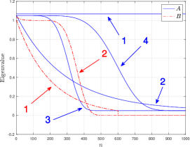
Figure 2: Different choices of spectra for $A$ and $B$ using the parameters in Table 1.

Next, we evaluate and compare the preconditioners in Table 2 and 3 for each combination of $A$ and $B$. We do not use any oversampling (i.e. $p=0$) to develop an understanding of the preconditioners in the simplest setting possible for relatively easy problems. In our randomised power range approximations ${{\widehat{S}}^{q}}\langle\Omega\rangle$ and ${{\tilde{S}}^{q}}\langle\Omega\rangle$, we use $q=2$. We compare against several algebraic preconditioners. Since $S$ in our setup is dense we do not use an incomplete Cholesky preconditioner. Instead, we shall use a partial Cholesky preconditioner (see e.g. [3]). Consider a formal partition of $S$:

$$S=\begin{bmatrix}S_{11}&S_{21}^{*}\\ S_{21}&S_{22}\end{bmatrix}.$$

Let $\begin{bmatrix}F_{11}\\ F_{21}\end{bmatrix}\in\mathbb{C}^{n\times r}$ denote the first $r$ columns of a Cholesky factor of $S$ using diagonal pivoting (for simplicity we ignore permutations). We let $D_{\textnormal{Schur}}$ denote the diagonal of whose elements are given by the Schur complement

$$S_{22}-S_{21}S_{11}^{-1}S_{21}^{*}$$

and form the preconditioner

$$P_{\texttt{pchol}}=\begin{bmatrix}F_{11}&\\ F_{21}&I_{n-r}\end{bmatrix}\begin{bmatrix}I_{r}&\\ &D_{\textnormal{Schur}}\end{bmatrix}\begin{bmatrix}F_{11}&F_{21}^{*}\\ &I_{n-r}\end{bmatrix}.$$

Hence, this can be considered a ”positive definite plus low rank” preconditioner. Another algebraic preconditioner is the symmetric Gauss-Seidel preconditioner [33] based on the decomposition

$$S=L+U+D$$

into the strictly lower triangular, upper triangular and diagonal elements:

$$P_{\textnormal{SGS}}=(D+L)D^{-1}(D+U).$$

This preconditioner requires access to the entire matrix, whereas $\widehat{S}_{r}$ (and the variations thereof) require only the factors of $A$. Here we analyse both strategies for synthetic data, but the practicality of either strategy may be entirely problem-dependent. The Jacobi preconditioner is simply the matrix consisting of the diagonal entries of $S$. The Python package scaled_preconditioners contains implementations of the preconditioners listed in the “Scaled” column of Table 2. We have used MATLAB R2022b [37] to generate the results shown in this paper.

Table 2: The preconditioners based on the structure $S=A+B$.

Approximation	Scaled	No scaling
Truncated SVD	$\widehat{S}_{r}$ (eq. (2b))	$\tilde{S}_{r}$ (eq. (2a))
Randomised SVD	${\widehat{S}}\langle\Omega\rangle$ (eq. (29))	${\tilde{S}}\langle\Omega\rangle:=A+{\widehat{B}}\langle\Omega\rangle)$
Rand. power range SVD	${{\widehat{S}}^{q}}\langle\Omega\rangle$ (eq. (32))	${{\tilde{S}}^{q}}\langle\Omega\rangle:=A+{{\widehat{B}}^{q}}\langle\Omega\rangle$
Nyström	${\widehat{S}}^{\text{Nys}}\langle\Omega\rangle$ (eq. (33a))	${\tilde{S}}^{\text{Nys}}\langle\Omega\rangle$ (eq. (33b)

Table 3: The algebraic preconditioners used in our numerical experiments.

Algebraic
Partial Cholesky
Symmetric Gauss-Seidel
Jacobi

6.1.2 Performance of Iterative Methods

For each combination of the spectra of $A$ and $B$ depicted in Figure 2 we generate 25 random instances of $O_{A}$ and $O_{B}$ in (37) to construct the system matrix $S=A+B$. For each of the preconditioners $\mathcal{P}$ in Table 2 and 3 we study the value of the Bregman divergence $\mathcal{D}_{\textnormal{LD}}(\mathcal{P},S)$, and the convergence behaviour of the PCG for the solution of $Sx=b$ with a relative tolerance of $10^{-7}$. Overall, we observed negligible variance in the results as a function of $O$ and $b$. We therefore only present results for one instance of bases for $A$ and $B$.

Table 4: PCG iteration counts for different instances of $A$ and $B$ and choice of preconditioner. We highlight the smallest iteration count across the preconditioners in bold.

Label

$\kappa_{2}(S)$

Iteration count

$A$

$B$

$I$

$P_{\texttt{pchol}}$

$P_{\textnormal{SGS}}$

Jacobi

$\tilde{S}_{r}$

${\tilde{S}}\langle\Omega\rangle$

${{\tilde{S}}^{q}}\langle\Omega\rangle$

${\tilde{S}}^{\text{Nys}}\langle\Omega\rangle$

$\widehat{S}_{r}$

${\widehat{S}}\langle\Omega\rangle$

${{\widehat{S}}^{q}}\langle\Omega\rangle$

${\widehat{S}}^{\text{Nys}}\langle\Omega\rangle$

[ head to column names, ]results_N=1000_r=300_tex.csv

Table 5: Bregman divergence values between the different preconditioners and choice of system matrix $S$ for different instances of $A$ and $B$. We highlight the smallest values across the preconditioners in bold.

The results are shown in Table 6.1.2 and 6.1.2. First we comment on the algebraic preconditioners. The simplest preconditioner, Jacobi, performs no better than unpreconditioned runs. The symmetric Gauss-Seidel preconditioner performs well overall, and for the case of constant diagonal $A$, PCG requires the fewest iterations with this preconditioner, and is the closest to $S$ in terms of Bregman divergence. In all other cases, $\widehat{S}_{r}$ performs better. Overall, the partial Cholesky preconditioner reduces the number of iterations required when compared to an unpreconditioned run, but not as effectively as the scaled preconditioners. As mentioned, the partial Cholesky preconditioner can be thought of as a diagonal plus low-rank matrix. The invariance property of the Bregman divergence was key to the theoretical results given in Section 3. By Theorem 1, $\widehat{S}_{r}$ is optimal in the Bregman divergence and $\widehat{S}_{r}^{-1}S$ has $\operatorname{rank}(B)-r+1$ distinct eigenvalues. In general, $P_{\texttt{pchol}}^{-1}S$ will have more distinct eigenvalues.

Next we comment on the preconditioners in Table 2. When the spectrum of $A$ is flat, Corollary 1 tells us the preconditioners $\widehat{S}_{r}$ and $\tilde{S}_{r}$ (and their respective variants) are identical. This is confirmed by the results seen in the top two rows of Table 6.1.2. As expected, most of the preconditioners perform similarly here as the problem is well-conditioned. In this case, the randomised power range preconditioners are almost as good as $\widehat{S}_{r}=\tilde{S}_{r}$ in terms of PCG convergence, with the results for the Nyström approximation being slightly worse. The standard randomised SVD can be seen be the worst choice in all cases. Analysing the Bregman divergence values in Table 6.1.2 leads to the same conclusion.

The rows of Table 6.1.2 and 6.1.2 where label $A=2$ show the results for the simple exponential decay of the eigenvalues of $A$ where we observe that by using the preconditioner $\widehat{S}_{r}$, PCG requires fewer iterations to achieve convergence for both instances of $B$, with the randomised power range preconditioner ${\widehat{S}}\langle\Omega\rangle^{q}$ almost achieving the same convergence. The results here are aligned with Theorem 1 which suggests that finding the correct basis for a preconditioner as well as matching the eigenvalues of $S$ has an impact on PCG convergence. Moreover, the Bregman divergence values in Table 6.1.2 appear to be a useful indicator of the PCG performance of the preconditioner, i.e., the smaller the divergence, the better the preconditioner performs. The inverse of $S$ is required to compute the Bregman log determinant divergence, so in practice the information in Table 6.1.2 is not available. To the best of our knowledge this divergence has not before been used to analyse preconditioners, so it is worthwhile developing an insight by studying smaller problems to support the theoretical results obtained above. For the labels $A=2$, $B=1$ means that the spectrum of $B$ decays exponentially while for $B=2$ it is mostly flat (cf. Figure 2). For $B=1$ we see that $\tilde{S}_{r}$ (and ${{\tilde{S}}^{q}}\langle\Omega\rangle$, by a small margin) leads to faster PCG convergence than ${\widehat{S}}^{\text{Nys}}\langle\Omega\rangle$, while the opposite is true when $B=2$. In the latter case, the spectrum of $G$ is more easily captured with an arbitrary sketching matrix, whereby the advantage of approximating $G$ is more profound, suggesting perhaps an effect similar to what was observed for the diagonal example in Section 2. As before, we see that the Bregman divergence values correlate with PCG performance. Interestingly, while ${\widehat{S}}\langle\Omega\rangle$ does not appear to be a good choice, our results for ${{\widehat{S}}^{q}}\langle\Omega\rangle$ show that a few power iterations can be used to great effect. We study the effect of sketching in more detail in Section 6.2.

It is instructive to look at rows where label $A=3$ and $A=4$ together, where the decay of $A$ is rapid but occurs at different points in the spectrum. By comparing these four cases of $A$ and $B$, we can develop some insight into how the sketching with $\Omega$ without any power iterations affects the results and how the randomised SVD approximations compare to the Nyström analogues. As before, $\widehat{S}_{r}$ and ${{\widehat{S}}^{q}}\langle\Omega\rangle$ are superior choices whereas ${\widehat{S}}\langle\Omega\rangle$, ${\tilde{S}}\langle\Omega\rangle$ and ${\tilde{S}}^{\text{Nys}}\langle\Omega\rangle$ lead to the slowest convergence. Here, the main difference in the results is the PCG convergence using ${\widehat{S}}^{\text{Nys}}\langle\Omega\rangle$, $\tilde{S}_{r}$, and ${{\tilde{S}}^{q}}\langle\Omega\rangle$. When the spectrum of $A$ and $B$ is mostly flat ($A=3$, $B=2$), PCG performs best using ${\widehat{S}}^{\text{Nys}}\langle\Omega\rangle$ as a preconditioner. Since we expect the approximation error owing to randomisation to be less pronounced, we see the benefits of the Nyström approximation over the randomised SVD preconditioner. In other words, the approximation of the $G$ matrix is less dependent on the realisation of the sketching matrix. A similar but less pronounced effect is seen when $A=3$, $B=2$. This is reflected in the Bregman divergence, where ${\widehat{S}}^{\text{Nys}}\langle\Omega\rangle$ are closer to $S$ in this nearness measure than $\tilde{S}_{r}$ or its variations.

Overall, these results suggest that while $\widehat{S}_{r}$ is at least as good a preconditioner as $\tilde{S}_{r}$ (and in all nontrivial cases, better), practical randomised numerical approximations thereof must be carried out with great care since we see that the ${\widehat{S}}\langle\Omega\rangle$ and ${\widehat{S}}^{\text{Nys}}\langle\Omega\rangle$ can be outperformed by $\tilde{S}_{r}$ depending on the spectrum of $A$ and $B$. In general, it appears that ${{\widehat{S}}^{q}}\langle\Omega\rangle$ is the best choice when the computation of $\widehat{S}_{r}$ is not an option. The comparison with algebraic preconditioners showed that when the structure of $S$ is known (i.e., $A$ is factorisable and we can make products with $B$), better preconditioners may be obtained by using the proposed framework. Furthermore, the preconditioners $P_{\texttt{pchol}}$ and $P_{\textnormal{SGS}}$ require access to the matrix $S$, which may not always be possible or convenient depending on the application at hand. In fact, the factor $Q$ is sufficient in order to construct a ”Scaled” preconditioner, since we assume we can make products with the remainder $S-QQ^{*}=B$, which lends itself better to cases where $S$ is a black box. Overall, the Bregman divergence appears to be a useful tool in suggesting how a preconditioner can perform in practice. A result such as Theorem 1 supports this analysis.

6.2 Effect of the Low Rank Approximation on the Bregman Divergence

To reinforce the intuition about the Bregman divergence we conclude by examining more closely how its terms are affected by the different low-rank approximations described previously. For simplicity, we now only consider the spectra given by $A=4$ and $B=1$ and set $n=100$, $m=60$, and $r=30$. Recall the definition in (8), where $X=U\operatorname{diag}(\lambda)U^{*}$ and $Y=V\operatorname{diag}(\theta)V^{*}$:

$$\mathcal{D}_{\textnormal{LD}}(X,Y)=\sum_{i=1}^{n}\sum_{j=1}^{n}(v_{i}^{*}u_{j})^{2}\Big{(}\frac{\lambda_{i}}{\theta_{j}}-\log\frac{\lambda_{i}}{\theta_{j}}-1\Big{)}.$$

Figure 3 and 4 show the terms of the Bregman divergence $\mathcal{D}_{\textnormal{LD}}(\mathcal{P},S)$ for each approximation $\mathcal{P}$ of $S$. The right column in these figures show that there is little difference between the terms $\frac{\lambda_{i}}{\theta_{j}}-\log\frac{\lambda_{i}}{\theta_{j}}-1$ in the definition of the divergence. Looking at the left columns of these figures suggests that the main contributing factor to the observed difference in Bregman divergence values in Table 6.1.2 lies in the approximation of the basis for $S$ expressed by the term $(v_{i}^{*}u_{j})^{2}$ in the expression above. In fact, we see that $\widehat{S}_{r}$ matches the first eigenvectors of $S$ perfectly by definition, and that the first $r$ eigenvectors of both ${{\widehat{S}}^{q}}\langle\Omega\rangle$ and ${\widehat{S}}\langle\Omega\rangle$ are almost collinear with those of $S$. This is not quite the case for ${\widehat{S}}^{\text{Nys}}\langle\Omega\rangle$, where we see the effect of the Nyström approximation. For the nonscaled preconditioners, we see in the left column that these approximations do not capture the basis in which the eigenvalues of $S$ are expressed, which is aligned with the PCG results seen in the rows $A=4$ and $B=1$ of Table 6.1.2.

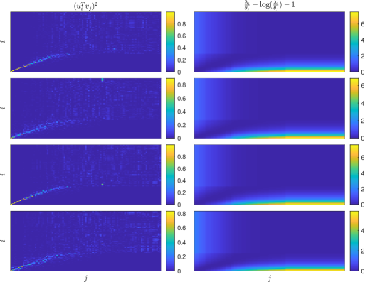
Figure 3: Bregman divergence terms for the nonscaled preconditioners. Top to bottom: $\tilde{S}_{r}$, ${\tilde{S}}\langle\Omega\rangle$, ${{\tilde{S}}^{q}}\langle\Omega\rangle$, ${\tilde{S}}^{\text{Nys}}\langle\Omega\rangle$.

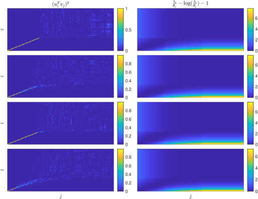
Figure 4: Bregman divergence terms for the scaled preconditioners. Top to bottom: $\widehat{S}_{r}$, ${\widehat{S}}\langle\Omega\rangle$, ${{\widehat{S}}^{q}}\langle\Omega\rangle$, ${\widehat{S}}^{\text{Nys}}\langle\Omega\rangle$.

6.3 Application to Variational Data Assimilation

Data assimilation is concerned with making predictions about the future state of a system provided noisy observations of its state along with prior knowledge given in the form of a model. Such predictions are only useful if they can be produced within a suitable timeframe, so efficient and scalable methods are important for practical forecasting [18]. The objective is to assimilate $N+1$ number of state variables $x_{i}\in\mathbb{R}^{n}$ at discrete times $t_{0}$, $\ldots$, $t_{N}$ given $N$ noisy observations $y_{i}\in\mathbb{R}^{m}$ at times $t_{1}$, $\ldots$, $t_{N}$, so that they approximately fit a forward propagation model while fitting with the observations. This implies the recurrence $x_{i}=\mathcal{M}_{i}(x_{i-1})$, $i=1,\ldots,N$, where $\mathcal{M}_{i}:\mathbb{R}^{n}\rightarrow\mathbb{R}^{n}$ is possibly nonlinear, subject to a baseline criterion $x_{0}=x_{0}^{B}+\xi_{0}$, where $\xi_{0}\in\mathcal{N}(0,B)$, $B\in\mathbb{R}^{n\times n}$, for a known $x_{0}^{B}$. Therefore, $x_{i}$ satisfies $y_{i}=\mathcal{H}_{i}x_{i}+\epsilon_{i}$, where $\epsilon_{i}\in\mathcal{N}(0,R_{i})$, $R_{i}\in\mathbb{R}^{m\times m}$ and $\mathcal{H}_{i}:\mathbb{R}^{n}\rightarrow\mathbb{R}^{m}$ is an (also possibly nonlinear) observation operator. The 4D variational data assimilation problem (4D-VAR) seeks to minimise the following functional:

$$J(x_{0})=\frac{1}{2}(x_{0}-x_{0}^{B})^{\top}B^{-1}(x_{0}-x_{0}^{B})+\frac{1}{2}\sum_{i=0}^{N}(y_{i}-\mathcal{H}_{i}(x_{i}))^{\top}R^{-1}(y_{i}-\mathcal{H}_{i}(x_{i})).$$ (38)

It is commonly acknowledged that the forecasting model $\mathcal{M}_{i}$ contains small errors or noise for which we do not want to overfit. We therefore replace the exact recurrence by $x_{i}=\mathcal{M}_{i}(x_{i-1})+\xi_{i}$, $i=1,\ldots,N$ for $\xi_{i}\in\mathcal{N}(0,Q_{i})$, $Q_{i}\in\mathbb{R}^{n\times n}$. This motivates the following weak constraint formulation [15] of (38):

$$J(x_{0}) =\frac{1}{2}(x_{0}-x_{0}^{B})^{\top}B^{-1}(x_{0}-x_{0}^{B})+\frac{1}{2}\sum_{i=0}^{N}(y_{i}-\mathcal{H}_{i}(x_{i}))^{\top}R_{i}^{-1}(y_{i}-\mathcal{H}_{i}(x_{i}))$$

$$+\frac{1}{2}\sum_{i=1}^{N}(x_{i}-\mathcal{M}_{i}(x_{i-1}))^{\top}Q_{i}^{-1}(x_{i}-\mathcal{M}_{i}(x_{i-1})).$$ (39)

This problem poses a challenge for computational scientists, as the size of many relevant assimilation problems posed as (39) is very large. To solve (39) we take an incremental approach and replace $J$ by a Gauss-Newton approximation [7]. This leaves a quadratic functional $\tilde{J}^{l}$ to be minimised for each iterate $\delta x^{l}=x^{l+1}-x^{l}$, where $l$ is the Gauss-Newton index:

$$\tilde{J}^{l}(\delta x^{l}) =(\delta x_{0}^{l}-b_{0}^{l})^{\top}B^{-1}(\delta x_{0}^{l}-b_{0}^{l})+\frac{1}{2}\sum_{i=0}^{N}(H^{l}_{i}\delta x_{i}^{l}-d_{i}^{l})^{\top}R_{i}^{-1}(H_{i}\delta x_{i}^{l}-d_{i}^{l})$$

$$+\frac{1}{2}\sum_{i=1}^{N}(M^{l}_{i}\delta x_{i-1}^{l}-\delta x_{i}^{l}-\eta_{i}^{l})^{\top}Q_{i}^{-1}(M^{l}_{i}\delta x_{i-1}^{l}-\delta x_{i}^{l}-\eta_{i}^{l}),$$ (40)

where we have used the substitutions $b_{0}^{l}=x_{0}^{l}-x_{0}^{B}$, $d_{i}^{l}=y_{i}-\mathcal{H}_{i}(x_{i}^{l})$, $\eta_{i}^{l}=x_{i}^{l}-\mathcal{M}_{i}(x_{i-1}^{l})$ and where $H^{l}_{i}$, $M^{l}_{i}$ are the tangent linear approximations at iterate $l$ of $\mathcal{H}_{i}$, $\mathcal{M}_{i}$, respectively. We rewrite (40) in a more compact way in (41) where we also drop the Gauss-Newton index:

$$\tilde{J}(\mathbf{\delta x}) =(\mathbf{L}\mathbf{\delta x}-\mathbf{b})^{\top}\mathbf{D}^{-1}(\mathbf{L}\mathbf{\delta x}-\mathbf{b})+(\mathbf{H}\mathbf{\delta x}-\mathbf{d})^{\top}\mathbf{R}^{-1}(\mathbf{H}\mathbf{\delta x}-\mathbf{d}),$$ (41)

by using the substitutions:

$$\mathbf{D}=\begin{bmatrix}B&&&\\ &Q_{1}&&\\ &&\ddots\\ &&&Q_{N}\end{bmatrix},\;\mathbf{L}=\begin{bmatrix}I&&\\ -M_{1}&I&\\ &\ddots&\\ &-M_{N}&I\end{bmatrix},$$ (42a)

$$\mathbf{R}=\begin{bmatrix}R_{0}&&\\ &\ddots&\\ &&R_{N}\end{bmatrix},\;\mathbf{H}=\begin{bmatrix}H_{0}&&\\ &\ddots&\\ &&H_{N}\end{bmatrix}.$$ (42b)

and:

$$\mathbf{b}=\begin{bmatrix}b_{0},\eta_{1},\ldots,\eta_{N}\end{bmatrix}^{\top},\quad\mathbf{d}=\begin{bmatrix}d_{0},\ldots,d_{N}\end{bmatrix}^{\top}.$$

Note that for $s=n(N+1)$ and $p=m(N+1)$, $\mathbf{D}\textnormal{,}\,\mathbf{L}\in\mathbb{R}^{s\times s}$, $\mathbf{R}\in\mathbb{R}^{p\times p}$, $\mathbf{H}\in\mathbb{R}^{p\times s}$, $\mathbf{b}\in\mathbb{R}^{s}$, $\mathbf{d}\in\mathbb{R}^{p}$ and we use $I$ to denote the identity matrix the dimension of which can be inferred from the context. Solving for the increment $\mathbf{\delta x}$ as in (41) in called the state formulation (see [14] for other approaches), where the matrix that we wish to invert is given by the Hessian of $\tilde{J}$:

$$\mathbf{S}=\mathbf{L}^{\top}\mathbf{D}^{-1}\mathbf{L}+\mathbf{H}^{\top}\mathbf{R}^{-1}\mathbf{H}.$$ (43)

In practice, the $s\times s$ system matrix in (43) can be very large and a good preconditioner is critical due to the small computational budget at operational scale relative to the problem size. In the next section we review a few key existing preconditioners for (43) and describe our proposed preconditioner based on the Bregman divergence framework.

6.3.1 Preconditioning the State Formulation of 4D VAR

Several preconditioners for (43) have therefore been proposed. Among these is the preconditioner

$$\mathbf{L}^{\top}\mathbf{D}^{-1}\mathbf{L},$$ (44)

see e.g. [22], which is simply the system matrix in (43) without the observation term. Approximations of $\mathbf{L}^{-1}$ have been used in the inverse of (44) and studied in [12]. In this section we shall not use any approximations of $\mathbf{L}$ as the objective is to demonstrate how (44) compares to other preconditioners that incorporate observation information in different ways. The preconditioner (44) can be updated with a low-rank term [34] leading to a preconditioner of the following form:

$$\tilde{\mathbf{S}}=\mathbf{L}^{\top}\mathbf{D}^{-1}\mathbf{L}+\mathbf{K}_{r}^{\top}\mathbf{K}_{r},$$ (45)

where $\mathbf{K}_{r}^{\top}\mathbf{K}_{r}$ is a rank $r<n$ truncated SVD of $\mathbf{H}^{\top}\mathbf{R}^{-1}\mathbf{H}$.

We note that $\mathbf{S}$ can be written as

$$\mathbf{S} =\mathbf{L}^{\top}(\mathbf{D}^{-1}+\mathbf{L}^{-\top}\mathbf{H}^{\top}\mathbf{R}^{-1}\mathbf{H}\mathbf{L}^{-1})\mathbf{L}$$

$$=\mathbf{L}^{\top}\mathbf{D}^{-{\frac{1}{2}}}(I+\mathbf{D}^{\frac{1}{2}}\mathbf{L}^{-\top}\mathbf{H}^{\top}\mathbf{R}^{-1}\mathbf{H}\mathbf{L}^{-1}\mathbf{D}^{\frac{1}{2}})\mathbf{D}^{-{\frac{1}{2}}}\mathbf{L}$$

$$=\mathbf{Q}(I+\mathbf{G})\mathbf{Q}^{\top},$$

where $\mathbf{Q}=\mathbf{L}^{\top}\mathbf{D}^{-{\frac{1}{2}}}$, $\mathbf{G}=\mathbf{Q}^{-1}\mathbf{H}^{\top}\mathbf{R}^{-1}\mathbf{H}\mathbf{Q}^{-\top}$. This leads to the following preconditioner which fits into the the framework presented in Section 3:

$$\hat{\mathbf{S}}_{r}=\mathbf{Q}(I+\mathbf{G}_{r})\mathbf{Q}^{\top},$$ (46)

where $\mathbf{G}_{r}$ is a rank $r$ truncation of $\mathbf{G}$. This is also referred to as a limited memory preconditioner in the literature [13, 9]. Since the number of observations is always smaller than the state space, $\operatorname{rank}(\mathbf{G})<n$ so by Theorem 2, the preconditioner $\hat{\mathbf{S}}_{r}$ minimises the condition number of the preconditioned system matrix among preconditioners of the form

$$\mathbf{L}^{\top}\mathbf{D}^{-1}\mathbf{L}+\mathbf{X},\quad\operatorname{rank}(\mathbf{X})\leq r.$$

As described in Section 5, it can be impractical to compute $\mathbf{G}_{r}$ when the size of the system is sufficiently large. Letting $\Omega\in\mathbb{R}^{s\times r}$ a Gaussian matrix of full rank we therefore define the Nyström variant of both (46) and (45):

$${\widehat{\mathbf{S}}}^{\text{Nys}}\langle\Omega\rangle=\mathbf{Q}(I+{\mathbf{G}}^{\text{Nys}}\langle\Omega\rangle)\mathbf{Q}^{\top},$$ (47a)

$${\tilde{\mathbf{S}}}^{\text{Nys}}\langle\Omega\rangle=\mathbf{L}^{\top}\mathbf{D}^{-1}\mathbf{L}+{(\mathbf{H}^{\top}\mathbf{R}^{-1}\mathbf{H})}^{\text{Nys}}\langle\Omega\rangle.$$ (47b)

Next, we compare the PCG performance of the preconditioners (44), (47a) and (47b) to an incomplete Cholesky preconditioner (since $\mathbf{S}$ will be sparse), for a specific problem instance.

6.3.2 Heat Equation

We now define the constituents (42) of the system matrix for assimilation of the heat equation:

$$\frac{\partial u}{\partial t}=\frac{\partial^{2}u}{\partial x^{2}},\quad t\in[0,\infty),\quad x\in[0,20].$$

We discretise the spatial operator by finite differences with $n=1000$ cells with size $\Delta x=2\cdot 10^{-2}$. We use a forward Euler scheme to discretise the time derivative with step size $\Delta t=10^{-4}$ for a total of $N+1=100$ discrete times, and let $r=\frac{\Delta t}{\Delta x^{2}}$ to define

$$M=\begin{bmatrix}0&0&0&0&\ldots&0&0\\ 0&1-2r&r&0&\ldots&0&0\\ 0&r&\ddots&\ddots&\ddots&\vdots&\vdots\\ \vdots&\vdots&\ddots&\ddots&\ddots&r&0\\ 0&\ldots&0&0&r&1-2r&0\\ 0&\ldots&0&0&0&0&0\end{bmatrix}$$

and set $M_{i}=M$, $i=1,\ldots,N$ to define $\mathbf{L}$. We set homogeneous Dirichlet boundary conditions in space for all time steps. We observe half of the state vector so $H_{i}\in\mathbb{R}^{m\times n}$ has a single unit entry per row. For $i=1,\ldots,N$ we set $(H_{i})_{m-j+1,j}=1$, $j=1,\ldots,m$ and all other elements set to zero to define $\mathbf{H}$. In practice, the covariance matrices $\mathbf{D}$ and $\mathbf{R}$ are typically ill-conditioned [35, 39]. To control the conditioning of $\mathbf{S}$ we therefore construct $\mathbf{D}$ by introducing a parameter $\tau_{\mathbf{D}}$ and sampling $s$ points in log space from $10^{-\tau_{\mathbf{D}}}$ to $10^{\tau_{\mathbf{D}}}$ and setting

$$\mathbf{D}^{-1}=\operatorname{diag}(10^{-\tau_{\mathbf{D}}},\ldots,10^{\tau_{\mathbf{D}}}).$$ (48)

We construct $\mathbf{R}^{-1}$ in a similar fashion and set use the values $\tau_{\mathbf{D}}=\tau_{\mathbf{R}}=1$. The parameters above lead to $\mathbf{S}$ in (43) being a $10^{5}\times 10^{5}$ matrix with condition number $\kappa_{2}(\mathbf{S})=8.1029\cdot 10^{5}$.

The purpose of this section is to compare various preconditioners for the Gauss-Newton iterate subproblems, so we generate $\mathbf{b}\in\mathbb{R}^{s}$ at random and focus on PCG for the solution of

$$\mathbf{S}\mathbf{\delta x}=\mathbf{b}.$$ (49)

For the preconditioners $\tilde{\mathbf{S}}_{r}$ and $\hat{\mathbf{S}}_{r}$ we look at three values of $r$ of varying size relative to $n$:

$$r=\lfloor n\times c\rfloor,\quad c\in\{0.005,0.02,0.04\}$$ (50)

corresponding to $0.05\%$, $2\%$ and $4\%$ of the problem size, respectively.

Figure 5 shows the PCG convergence for the preconditioners above along with the preconditioner $\mathbf{L}^{\top}\mathbf{D}^{-1}\mathbf{L}$, an incomplete Cholesky preconditioner and an unpreconditioned run of the conjugate gradient metod. Table 6.3.2 shows the the computation time and relvative residual achieved for these runs. It is clear that the preconditioner ${\widehat{\mathbf{S}}}^{\text{Nys}}\langle\Omega\rangle$ greatly outperforms ${\tilde{\mathbf{S}}}^{\text{Nys}}\langle\Omega\rangle$ for the same value of $r$. While increasing the rank $r$ leads to faster convergence for both approaches, we clearly see that the scaled approach performs much better. We even see that ${\widehat{\mathbf{S}}}^{\text{Nys}}\langle\Omega\rangle$ with a rank 500 truncation outperforms ${\tilde{\mathbf{S}}}^{\text{Nys}}\langle\Omega\rangle$ for a rank 4000 truncation of the observation term. This supports the theory developed above. Neither the preconditioner $\mathbf{L}^{\top}\mathbf{D}^{-1}\mathbf{L}$ or the incomplete Cholesky preconditioners are close to reaching a small residual, as we also see from Figure 5. We emphasise that there may be problem instances for which these approaches could be viable.

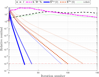
Figure 5: PCG iteration count for the solution (49) for different preconditioners. Thicker lines correspond to higher values of the truncation rank $r$ in (50).

Table 6: Timings, residuals and PCG iteration counts for the solution of (49) for various preconditioners. The residual tolerance is $10^{-6}$ and the iteration limit is $150$.

One of the limitations of our framework is that $A$ in $S=A+B$ must be known and factorisable. In the setting above, $A=\mathbf{L}^{\top}\mathbf{D}^{-1}\mathbf{L}$, which may be difficult to factorise for certain forward operators and covariances. As mentioned, the literature has explored adopting a preconditioner of the form (44) but substituting $\mathbf{L}$ for an approximation whose inverse is easier to compute [14]. [8] adopts a similar methodology by approximating $\mathbf{L}^{-1}$ by an identity plus low-rank matrix. Both approaches result in the construction of an approximate positive definite $\tilde{A}\approx A$ which is easier to store or parallelise. As mentioned in Section 3.1, we extend the Bregman divergence framework to handle approximate factorisations $\tilde{A}\approx A$ in a sequel.

7 Summary & Outlook

In this paper, we have presented several preconditioners for solving $Sx=b$ where the matrix $S$ is a sum of $A\in{\mathbb{H}^{n}_{++}}$ and $B\in{\mathbb{H}^{n}_{+}}$. The first proposed preconditioner, $\widehat{S}_{r}$ in (2b), is chosen as a sum of a $A$ and a low-rank matrix, is the minimiser of a Bregman divergence. We have shown how this preconditioner can be recovered from a scaled Frobenius norm minimisation problem, and that, when $\operatorname{rank}(B)<n$, it is optimal in the sense that it minimises the condition number of the preconditioned matrix for preconditioners on its form, i.e., positive definite plus low rank. We have also presented variants of $\widehat{S}_{r}$ based on randomised low-rank approximations. We also established a link between the Bregman divergence and the Nyström approximation. The equivalence between single pass randomised SVD and the Nyström approximation was also, to the best of the authors’ knowledge, not documented before. Our numerical experiments illustrate how our theoretical results vary for different choices of $A$ and $B$, and for different practical choices of low-rank approximations, i.e., randomised, randomised with power iterations, and a randomised Nyström approximation. We also illustrated the potential of our proposed framework for preconditioning a system stemming from a variational data assimilation problem.

The work in this paper offers many avenues for future research. The invariance property of the Bregman divergence has shown to be a valuable property in interpreting the quality of the different preconditioners studied in this work. Knowledge of the structure of $S$ as the sum of $A$ and $B$ was essential in utilising this invariance cf. (9). Understanding the choice of splitting of the matrix $S$ discussed in Section 3.1 could help in developing new approximation methods, for instance when the positive definite part of $S$ is not known or easily factorisable. In [25], the authors developed a preconditioner based on a low-accuracy LU factorisation for ill-conditioned systems, which could yield insights in this direction. We could also investigate preconditioners of other forms, such as either hierarchical matrices, leading to different constraints in a Bregman divergence minimisation problem such as in Section 3.2. It could also be fruitful to see to which extent the framework introduced here generalises approaches such as in [17]. The link between the Bregman divergence and the Nyström approximation may also help to explain why this approximation is suitable for a given application since, as we saw in Section 6, it always appears to improve PCG convergence over a randomised SVD. However, if the computational budget of a given application allows for a randomised power range approximation, this effort appears to be well compensated in terms of PCG performance. Saddle-point formulations of the inner loop 4D-VAR problem have also been studied due to their potential for parallelisation [36, 14, 34]. Low-rank approaches have been explored in this context before [19], so it would be natural to adapt the framework presented above to this setting.

Other divergences commonplace in information geometry could also be interesting to analyse, e.g., the Itakura-Saito divergence or the divergence associated with the negative Shannon entropy. Deeper connections could be sought between this domain and other problems in numerical linear algebra beyond preconditioning.

8 Acknowledgements

This work was supported by the Novo Nordisk Foundation under grant number NNF20OC0061894.

Appendix A Synthetic Data: Generalised Eigenvalues

In Figure 6 we show the generalised eigenvalues for various preconditioners using the experimental setup from Section 6.1.

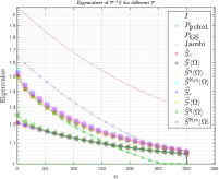
(a) $A=1$, $B=1$.

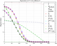
(b) $A=1$, $B=2$.

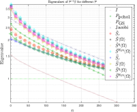
(c) $A=2$, $B=1$.

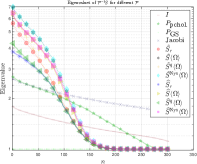
(d) $A=2$, $B=2$.

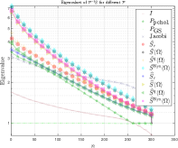
(e) $A=3$, $B=2$.

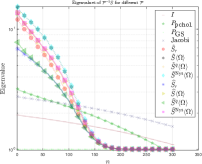
(f) $A=3$, $B=1$.

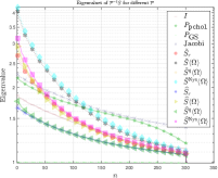
(g) $A=4$, $B=1$.

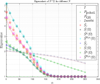
(h) $A=4$, $B=2$.

Figure 6: Generalised eigenvalues for various preconditioners $P$. The graphs correspond to the choices of $A$ and $B$ given by the label in Table 1.

References

- [1] S.-i. Amari, Information geometry and its applications, vol. 194, Springer, 2016.
- [2] S.-i. Amari and A. Cichocki, Information geometry of divergence functions, Bulletin of the polish academy of sciences. Technical sciences, 58 (2010), pp. 183–195.
- [3] S. Bellavia, J. Gondzio, and B. Morini, A matrix-free preconditioner for sparse symmetric positive definite systems and least-squares problems, SIAM Journal on Scientific Computing, 35 (2013), pp. A192–A211.
- [4] M. Benzi, G. H. Golub, and J. Liesen, Numerical solution of saddle point problems, Acta numerica, 14 (2005), pp. 1–137.
- [5] L. M. Bregman, The relaxation method of finding the common point of convex sets and its application to the solution of problems in convex programming, USSR computational mathematics and mathematical physics, 7 (1967), pp. 200–217.
- [6] P. J. Bushell and G. B. Trustrum, Trace inequalities for positive definite matrix power products, Linear Algebra and its Applications, 132 (1990), pp. 173–178.
- [7] P. Courtier, J.-N. Thépaut, and A. Hollingsworth, A strategy for operational implementation of 4D-Var, using an incremental approach, Quarterly Journal of the Royal Meteorological Society, 120 (1994), pp. 1367–1387.
- [8] I. Daužickaitė, A. S. Lawless, J. A. Scott, and P. J. van Leeuwen, On time-parallel preconditioning for the state formulation of incremental weak constraint 4D-Var, Quarterly Journal of the Royal Meteorological Society, 147 (2021), pp. 3521–3529.
- [9] I. Daužickaitė, A. S. Lawless, J. A. Scott, and P. J. Van Leeuwen, Randomised preconditioning for the forcing formulation of weak-constraint 4D-Var, Quarterly Journal of the Royal Meteorological Society, 147 (2021), pp. 3719–3734.
- [10] I. S. Dhillon and J. A. Tropp, Matrix nearness problems with Bregman divergences, SIAM Journal on Matrix Analysis and Applications, 29 (2008), pp. 1120–1146.
- [11] P. Drineas, M. W. Mahoney, and N. Cristianini, On the Nyström method for approximating a Gram matrix for improved kernel-based learning., Journal of Machine Learning Research, 6 (2005).
- [12] A. El-Said, Conditioning of the weak-constraint variational data assimilation problem for numerical weather prediction, PhD thesis, University of Reading, 2015.
- [13] M. Fisher, S. Gratton, S. Gürol, Y. Trémolet, and X. Vasseur, Low rank updates in preconditioning the saddle point systems arising from data assimilation problems, Optimization Methods and Software, 33 (2018), pp. 45–69.
- [14] M. Fisher and S. Gürol, Parallelization in the time dimension of four-dimensional variational data assimilation, Quarterly Journal of the Royal Meteorological Society, 143 (2017), pp. 1136–1147.
- [15] M. Fisher, Y. Tremolet, H. Auvinen, D. Tan, and P. Poli, Weak-constraint and long-window 4D-Var, ECMWF Reading, UK, 2012.
- [16] Z. Frangella, P. Rathore, S. Zhao, and M. Udell, SketchySGD: Reliable stochastic optimization via robust curvature estimates, arXiv preprint arXiv:2211.08597, (2022).
- [17] Z. Frangella, J. A. Tropp, and M. Udell, Randomized Nyström preconditioning, arXiv preprint arXiv:2110.02820, (2021).
- [18] M. A. Freitag, Numerical linear algebra in data assimilation, GAMM-Mitteilungen, 43 (2020), p. e202000014.
- [19] M. A. Freitag and D. L. H. Green, A low-rank approach to the solution of weak constraint variational data assimilation problems, Journal of Computational Physics, 357 (2018), pp. 263–281.
- [20] A. Gittens and M. W. Mahoney, Revisiting the Nyström method for improved large-scale machine learning, The Journal of Machine Learning Research, 17 (2016), pp. 3977–4041.
- [21] G. H. Golub and C. F. Van Loan, Matrix Computations, Johns Hopkins University Press, 2013.
- [22] S. Gratton, S. Gürol, E. Simon, and P. L. Toint, Guaranteeing the convergence of the saddle formulation for weakly constrained 4D-Var data assimilation, Quarterly Journal of the Royal Meteorological Society, 144 (2018), pp. 2592–2602.
- [23] A. Greenbaum, Iterative methods for solving linear systems, SIAM, 1997.
- [24] N. Halko, P.-G. Martinsson, and J. A. Tropp, Finding structure with randomness: Probabilistic algorithms for constructing approximate matrix decompositions, SIAM review, 53 (2011), pp. 217–288.
- [25] N. J. Higham and T. Mary, A new preconditioner that exploits low-rank approximations to factorization error, SIAM Journal on Scientific Computing, 41 (2019), pp. A59–A82.
- [26] R. A. Horn and C. R. Johnson, Topics in matrix analysis, Cambridge university press, 1994.
- [27] B. Kulis, M. A. Sustik, and I. S. Dhillon, Low-rank kernel learning with Bregman matrix divergences., Journal of Machine Learning Research, 10 (2009).
- [28] P.-G. Martinsson, Randomized methods for matrix computations, The Mathematics of Data, 25 (2019), pp. 187–231.
- [29] P.-G. Martinsson and J. A. Tropp, Randomized numerical linear algebra: Foundations and algorithms, Acta Numerica, 29 (2020), pp. 403–572.
- [30] Y. Nakatsukasa, Fast and stable randomized low-rank matrix approximation, arXiv preprint arXiv:2009.11392, (2020).
- [31] C. E. Rasmussen, C. K. Williams, et al., Gaussian processes for machine learning, vol. 1, Springer, 2006.
- [32] R. T. Rockafellar, Convex Analysis, vol. 11, Princeton University Press, 1997.
- [33] J. Scott and M. Tůma, Algorithms for sparse linear systems, Springer Nature, 2023.
- [34] J. Tabeart and D. Palitta, Stein-based preconditioners for weak-constraint 4D-Var, Numerical Methods for Large Scale Problems, p. 50.
- [35] J. M. Tabeart, S. L. Dance, A. S. Lawless, N. K. Nichols, and J. A. Waller, New bounds on the condition number of the Hessian of the preconditioned variational data assimilation problem, Numerical Linear Algebra with Applications, 29 (2022), p. e2405.
- [36] J. M. Tabeart and J. W. Pearson, Saddle point preconditioners for weak-constraint 4d-var, arXiv preprint arXiv:2105.06975, (2021).
- [37] The MathWorks Inc., MATLAB, 2022. Version: 9.13.0 (R2022b).
- [38] J. Wenger, G. Pleiss, P. Hennig, J. Cunningham, and J. Gardner, Preconditioning for scalable Gaussian process hyperparameter optimization, in International Conference on Machine Learning, PMLR, 2022, pp. 23751–23780.
- [39] P. Weston, W. Bell, and J. Eyre, Accounting for correlated error in the assimilation of high-resolution sounder data, Quarterly Journal of the Royal Meteorological Society, 140 (2014), pp. 2420–2429.
- [40] C. Williams and M. Seeger, Using the Nyström method to speed up kernel machines, Advances in neural information processing systems, 13 (2000).
- [41] D. P. Woodruff et al., Sketching as a tool for numerical linear algebra, Foundations and Trends® in Theoretical Computer Science, 10 (2014), pp. 1–157.
- [42] N. Zhang and P. Shen, Constraint preconditioners for solving singular saddle point problems, Journal of computational and applied mathematics, 238 (2013), pp. 116–125.
- [43] S. Zhao, Z. Frangella, and M. Udell, NysADMM: faster composite convex optimization via low-rank approximation, in International Conference on Machine Learning, PMLR, 2022, pp. 26824–26840.