Homogenization of line tension energies

Abstract: We prove an homogenization result, in terms of $\Gamma$-convergence, for energies concentrated on rectifiable lines in $\mathbb{R}^{3}$ without boundary. The main application of our result is in the context of dislocation lines in dimension $3$. The result presented here shows that the line tension energy of unions of single line defects converge to the energy associated to macroscopic densities of dislocations carrying plastic deformation. As a byproduct of our construction for the upper bound for the $\Gamma$-Limit, we obtain an alternative proof of the density of rectifiable $1$-currents without boundary in the space of divergence free fields.

Keywords

Gamma convergence, dislocations, divergence free fields, homogenization.

1 Introduction

In this paper we prove an homogenization result for energies of the form

$$\int_{\gamma}\psi(b,t)d\mathcal{H}^{1},$$ (1.1)

where $\mu=b\otimes t\mathcal{H}^{1}\mathbin{\vrule height=6.88889pt,depth=0.0pt,width=0.55974pt\vrule height=0.55974pt,depth=0.0pt,width=5.59721pt}\gamma$ is a divergence free matrix valued measure, $\gamma\subset\mathbb{R}^{3}$ is a $1$-rectifiable set, and $t$ its tangent. The vector $b$ is a multiplicity which belongs to a discrete lattice $\mathcal{B}$ in $\mathbb{R}^{N}$, with $N\geq 2$, and will also be called the Burgers vector of $\mu$. Here $\mathcal{M}_{df}^{1}(\Omega;\mathcal{B}\times\mathbb{S}^{2})$ denotes the set of such measures, where $\Omega\subset\mathbb{R}^{3}$ is an open bounded and regular set.

We consider the following scaled version of the energy in (1.1)

$$E_{\sigma}(\mu):=\begin{cases}\displaystyle{\int_{\gamma\cap\Omega}\sigma\psi\left(\dfrac{b}{\sigma},t\right)d\mathcal{H}^{1}}\quad&\hbox{if }\ \mu=b\otimes t\mathcal{H}^{1}\mathbin{\vrule height=6.88889pt,depth=0.0pt,width=0.55974pt\vrule height=0.55974pt,depth=0.0pt,width=5.59721pt}\gamma\in\mathcal{M}_{df}^{1}(\Omega;\sigma\mathcal{B}\times\mathbb{S}^{2}),\\ +\infty&\hbox{otherwise}.\end{cases}$$ (1.2)

Under some mild assumptions on the density $\psi$ we study the asymptotics of $E_{\sigma}$ in terms of $\Gamma$-convergence with respect to the weak$*$ topology of measures. The main result of the paper is that the limiting energy takes the form

$$E_{0}(\mu)=\begin{cases}\displaystyle\int_{\Omega}g\left(\dfrac{d\mu(x)}{d\|\mu\|}\right)d\|\mu\|\quad&\hbox{if }\mu\in[\mathcal{M}(\Omega)]^{N\times 3},\ \operatorname*{div}\mu=0,\\ {+\infty}&\hbox{otherwise},\end{cases}$$ (1.3)

where $g:\mathbb{R}^{N\times 3}\longrightarrow[0,+\infty)$ is a convex $1$-homogeneous function defined in terms of the density $\psi$ (see Theorem 2.5 for the exact statement).

Our result extends the result in [8], where the same problem is treated in dimension $2$, i.e., $\Omega\subset\mathbb{R}^{2}$, and from which we borrow several ideas for the proof. The main difference is that in dimension $2$ the support of the measures in $\mathcal{M}_{df}^{1}(\Omega;\mathcal{B}\times\mathbb{S}^{1})$ has codimension $1$, so that the energy in (1.1) reduces to a functional defined in the space of $SBV$ functions with values in $\mathcal{B}$ (and the measure $\mu$ is nothing but the rotated gradient of the phase field $u$). This allow the authors to use tools from the Calculus of Variations for functionals defined on partitions and therefore in $SBV$ (see [1]).

In dimension larger than $2$ there is no phase field describing the admissible configuration, so we use techniques of geometric measure theory and the analysis of functionals defined on rectifiable currents (rephrased in terms of the measures in $\mathcal{M}_{df}^{1}(\Omega;\mathcal{B}\times\mathbb{S}^{2})$). Energies of the form (1.1) have been studied in [6] where the authors give necessary and sufficient conditions for the lower semicontinuity of such functionals.

The major difficulty in the proof of the $\Gamma$-convergence is the construction for the upper bound. Implementing a standard density argument we first need to reduce to the case of measures absolutely continuous with respect to Lebesgue and having piecewise constant density. This step requires to prove that such measures are dense in energy for the limiting functional $E_{0}$. The second key ingredient of the proof is then an ad hoc construction which allows to approximate divergence free piecewise constant fields with measures concentrated on polyhedral closed curves and optimal energy. As a byproduct of the construction for the recovery sequence we thus obtain a different proof of the approximation of divergence free vector fields by means of measures defined on closed curves (see Theorem 3.5). Stated by J. Bourgain and H. Brezis in [3] in the context of solenoidal charges in the sense of Smirnov (see [21]), this density result is proved in [15] with respect to the strict topology of measures.

The main motivation for our analysis is the study of line defects in a $3$-dimensional crystal, the so called dislocations. At a mesoscopic scale (larger than the microscopic lattice spacing) they are indeed identified with line objects carrying a vector multiplicity belonging to the lattice, so that they can be represented as measures belonging to $\mathcal{M}_{df}^{1}(\Omega;\mathcal{B}\times\mathbb{S}^{2})$. The divergence free constraint is reminiscent of the topological nature of these defects. At this level one can associate to each dislocation a line tension energy, i.e., an energy with the same form of (1.1). Such energies can in turn be derived from more fundamental models. For example, in [10], [13], and [5] the authors deduce the line tension model accounting for the elastic distortion in the material induced by the presence of dislocations. See also [19], [20], [11], and [18] for a similar derivation in dimension 2 for cylindrical geometry where dislocations are viewed as point defects. Similarly, this type of line tension model can also be derived under the assumption that the line defects are contained in a given (slip) plane as limit of nonlocal phase transition energies (in the spirit of the Cahn Hilliard energies for liquid-liquid phase transtions), known in the literature of dislocations as (generalised) Nabarro-Peirls models (see [7] and the references therein). The natural representation of the line energy here is given by functionals defined on the space of $BV$ functions with values in a discrete group, so that dislocations are identified by the jump set of such functions, see [9].

In this paper we are interested in the case of a large number of dislocations on a macroscopic scale. The interest of this case lying in the fact that a large quantity of dislocations is responsible for plastic deformation in the material (see [8] for a more complete analysis). In particular, starting from the rescaled version of the line tension energy defined in (1.2), we are interested in recovering an effective energy for a large system of dislocations on a scale at which they can be seen as diffused. In this respect our limiting energy $E_{0}$ can be understood as the macroscopic (self) energy associated to a continuous distribution of dislocations.

The result presented in here is also a crucial step for a derivation of a macroscopic model for plasticity accounting for the presence of defects in the same spirit of [12]. The derivations of such macroscopic models as limit of elastic energies for incompatible fields, under proper energy scalings, will appear in a forthcoming paper.

The structure of the paper is as follows: in Section 2 we give preliminary definitions and recall some known results. In Section 2.3 we state the main result and present the proof of the lower bound. In Section 3 we present the approximation results needed for the upper bound, the latter being proved in Section 4.

2 Preliminaries and statement of the main result

We first set all the notation needed for the statement and proof of our main result. Unless further specified, in what follows $\Omega$ is a bounded open set of $\mathbb{R}^{n}$ with Lipschitz boundary. In what follows, without loss of generality we will assume $\mathcal{B}=\mathbb{Z}^{N}$, for $N\geq 1$.

2.1 Configurations

We start with the set of admissible configurations. In what follows we will denote with $[\mathcal{M}(\Omega)]^{N\times n}$ the space of bounded Radon measures with values in $\mathbb{R}^{N\times n}$. The space $\mathcal{M}^{1}(\Omega;\mathcal{S}\times\mathbb{S}^{n-1})$ will denote the set of measures in $[\mathcal{M}(\Omega)]^{N\times n}$ of the form

$$\mu=\theta\otimes\tau\mathcal{H}^{1}\mathbin{\vrule height=6.88889pt,depth=0.0pt,width=0.55974pt\vrule height=0.55974pt,depth=0.0pt,width=5.59721pt}\gamma,$$ (2.1)

where $\gamma\subset\mathbb{R}^{n}$ is a $1$-rectifiable set with tangent vector $\tau\in\mathbb{S}^{n-1}$ defined $\mathcal{H}^{1}$ a.e. on $\gamma$, $\mathcal{S}\subset\mathbb{R}^{N}$ is a generic subset, and $\theta\in[L^{1}(\gamma,\mathcal{H}\mathbin{\vrule height=6.88889pt,depth=0.0pt,width=0.55974pt\vrule height=0.55974pt,depth=0.0pt,width=5.59721pt}\gamma)]^{N}$ is such that $\theta(x)\in\mathcal{S}$ for $\mathcal{H}^{1}$-a.e. $x\in\gamma$. We remark that in most cases we will consider the set $\mathcal{S}$ to be a discrete lattice that spans $\mathbb{R}^{N}$ but for notational purposes it is convenient to give the above definition for general sets. We also observe that although the main result, Theorem 2.5, is stated for the case $n=3$, in Section $3$ we prove an approximation result which holds in any dimension, hence it is convenient to give the relevant definitions for an arbitrary dimension $n\geq 2$.

We say that a measure in $[\mathcal{M}(\Omega)]^{N\times n}$ is divergence free if it is row-wise divergence free, i.e., if the following holds true

$$\int_{\Omega}\sum_{j=1}^{n}\partial_{j}\varphi d\mu_{ij}=0\qquad\forall\varphi\in C_{0}^{\infty}(\Omega),\qquad\forall i=1,\cdots,N.$$

The subset of $\mathcal{M}^{1}(\Omega;\mathcal{S}\times\mathbb{S}^{n-1})$ (and $[\mathcal{M}(\Omega)]^{N\times n}$) of divergence free measures will be denoted by $\mathcal{M}_{df}^{1}(\Omega;\mathcal{S}\times\mathbb{S}^{n-1})$ (respectively $[\mathcal{M}(\Omega)]_{df}^{N\times n}$). Note that, if $G\in[L^{1}(\Omega)]^{N\times n}$ and $\mu=G\mathcal{L}^{n}\in[\mathcal{M}(\Omega)]^{N\times n}$ with $\mathcal{L}^{n}$ the $n$-dimensional Lebesgue measure, then $\mathop{\mathrm{div}}G=0$ in the sense of distributions if and only if $\mu\in\mathcal{[}\mathcal{M}(\Omega)]_{df}^{N\times n}$.

We say that a measure $\mu\in\mathcal{M}^{1}(\Omega;\mathcal{S}\times\mathbb{S}^{n-1})$ is polyhedral if its support if formed by a finite number of straight closed segments.

Remark 2.1.

Given a measure $\mu=b\otimes t\mathcal{H}^{1}\mathbin{\vrule height=6.88889pt,depth=0.0pt,width=0.55974pt\vrule height=0.55974pt,depth=0.0pt,width=5.59721pt}\gamma\in\mathcal{M}^{1}(\Omega;\mathbb{Z}^{N}\times\mathbb{S}^{n-1})$, where $b\in\mathbb{Z}^{N}$ is constant and $\gamma\in[\operatorname{Lip}([0,1])]^{n}$ is a curve such that $\gamma^{\prime}=t$, it holds that

$$\langle\mu,\nabla\varphi\rangle=\langle b,\varphi(\gamma(1))-\varphi(\gamma(0))\rangle,\ \ \forall\varphi\in[C_{c}^{1}(\mathbb{R}^{n})]^{N},$$ (2.2)

hence it must be

$$\mathop{\mathrm{div}}\mu=b\delta_{\gamma(0)}-b\delta_{\gamma(1)},$$ (2.3)

where $b\delta_{a}\in[\mathcal{M}(\Omega)]^{N}$ is a Dirac delta centered at $a\in\Omega$ with multiplicity $b$. Accordingly we say that $\mu$ carries a mass of $b$ at $\gamma(0)$ and a mass of $-b$ at $\gamma(1)$, where the sign depends on the orientation $t$. In particular for such a measure to be divergence free in $\Omega$, the curve $\gamma$ must not have endpoints contained in $\Omega$.

Remark 2.2.

If $\Omega$ is a simply connected domain, measures in $\mathcal{M}_{df}^{1}(\Omega;\mathbb{Z}^{N}\times\mathbb{S}^{n-1})$ can be extended to measures on the whole of $\mathbb{R}^{n}$ that can be characterized as measures concentrated on unions of countably many closed Lipschitz loops with constant multiplicity in $\mathbb{Z}^{N}$ (see [6], Theorem 2.5, for the precise statement given in terms of $1$-rectifiable currents).

The set $\mathcal{M}_{df}^{1}(\Omega;\mathbb{Z}^{N}\times\mathbb{S}^{2})$ represents the set of admissible configurations for the class of energies under consideration.

2.2 Energy densities and their main properties

Here we recall the main properties of the class of energy densities

$$\psi:\mathbb{Z}^{N}\times\mathbb{S}^{2}\longrightarrow[0,+\infty).$$

The $\mathcal{H}^{1}$-elliptic envelope of $\psi$ is the function $\psi^{rel}$ obtained by solving, for any $b\in\mathbb{Z}^{N}$ and $t\in\mathbb{S}^{2}$, the cell problem

$$\psi^{\mathrm{rel}}(b,t):=\inf\Big{\{} \int_{\gamma}\psi(\theta,\tau)d\mathcal{H}^{1}:\mu=\theta\otimes\tau\mathcal{H}^{1}\mathbin{\vrule height=6.88889pt,depth=0.0pt,width=0.55974pt\vrule height=0.55974pt,depth=0.0pt,width=5.59721pt}\gamma\in\mathcal{M}_{df}^{1}(B_{1};\mathbb{Z}^{N}\times\mathbb{S}^{n-1}),$$ (2.4)

$$\operatorname{supp}\left(\mu-b\otimes t\mathcal{H}^{1}\mathbin{\vrule height=6.88889pt,depth=0.0pt,width=0.55974pt\vrule height=0.55974pt,depth=0.0pt,width=5.59721pt}\left(\mathbb{R}t\cap B_{1/2}\right)\right)\subset\subset B_{1/2}\Big{\}},$$

where $B_{r}=B_{r}(0)$ denotes a ball of radius $r$ and center 0. We say that $\psi$ is $\mathcal{H}^{1}$-elliptic if $\psi^{rel}=\psi$ (see [6]).

We will assume that $\psi$ is $\mathcal{H}^{1}$-elliptic and we extend it to the whole of $\mathbb{R}^{N}\times\mathbb{S}^{2}$ by setting $\psi(b,t)=+\infty$ for all $b\in\mathbb{R}^{N}\smallsetminus\mathbb{Z}^{N}$. Further, we assume that

$$\psi(b,t)\geq c\,|b|\qquad\forall\ b\,\in\mathbb{Z}^{N}\smallsetminus\{0\}\hbox{ and }t\in\mathbb{S}^{2}.$$ (2.5)

Moreover we recall that $\mathcal{H}^{1}$-ellipticity implies that $\psi$ is subattidive and has linear growth at infinity in the first entry, i.e., for all $b,b^{\prime}\in\mathbb{R}^{N}$ and $t\in\mathbb{S}^{2}$ it satisfies

$$\psi(b+b^{\prime},t)\leq\psi(b,t)+\psi(b^{\prime},t)\qquad\hbox{and }\qquad\psi(b,t)\leq\overline{c}\,|b|,$$ (2.6)

for some positive constant $\overline{c}$, see [6, Lemma 3.2 (iii) and (iv)].

The recession function $\psi_{\infty}:\mathbb{R}^{N}\times\mathbb{S}^{2}\rightarrow$ $[0,\infty]$ of $\psi$ is given by

$$\psi_{\infty}(b,t):=\liminf_{s\rightarrow+\infty}\frac{1}{s}\psi(sb,t).$$ (2.7)

This is a crucial ingredient in order to determine the effective energy density of the limiting energy $E_{0}$. For the readers’ convenience we now recall some of the main properties of $\psi_{\infty}$ as they are proved in [8].

Proposition 2.3.

Let $\psi:\mathbb{R}^{N}\times\mathbb{S}^{2}\to\mathbb{R}\cup\{+\infty\}$ be $\mathcal{H}^{1}$-elliptic, satifying (2.5) and such that $\psi(b,t)=+\infty$ if $b\in\mathbb{R}^{N}\setminus\mathbb{Z}^{N}$. Let $\psi_{\infty}$ be its recession function. Then the following hold:

1. $\psi_{\infty}(\cdot,t)$ is positively $1$-homogeneous for all $t\in\mathbb{S}^{2}$;

2. Let $\mathcal{Q}=\left\{\lambda z:\lambda>0,z\in\mathbb{Z}^{N}\right\}$, then $\psi_{\infty}(b,t)=+\infty$ if $b\in\mathbb{R}^{N}\smallsetminus\mathcal{Q}$, and $\psi_{\infty}(b,t)\leq c\,|b|$ for $b\in\mathcal{Q}$;

3. Let $b\in\mathbb{R}^{N},t\in\mathbb{S}^{2}$, for any sequence $z_{j}\in\mathbb{Z}^{N}$ such that $\left|z_{j}\right|\rightarrow+\infty$ and $z_{j}/\left|z_{j}\right|\rightarrow b/|b|$ one has

   $$\lim_{j\rightarrow+\infty}\frac{1}{\left|z_{j}\right|}\psi\left(z_{j},t\right)=\frac{1}{|b|}\psi_{\infty}(b,t).$$

The proof of property (i) is immediate, while properties (ii) and (iii) can be found in [8], Lemma 3.3 and 3.4 respectively.

Finally we define the function $g:\mathbb{R}^{N\times 3}\longrightarrow[0,+\infty)$, which provides the effective energy density, as the convex envelope of

$$g_{\infty}(A)=\begin{cases}\psi_{\infty}(b,t)\quad&\hbox{if }A=b\otimes t,\ \ b\in\mathbb{R}^{N},\ \ t\in\mathbb{S}^{2},\\ {+\infty}&\hbox{otherwise},\end{cases}$$ (2.8)

i.e., $g(A)=g^{**}_{\infty}(A)$. Some important properties of $g$ are described in the following

Lemma 2.4.

The function $g$ is continuous, $1$-homogeneous, and there are $c_{1},c_{2}>0$ such that

$$c_{1}|A|\leq g(A)\leq c_{2}|A|,$$

for all matrices $A\in\mathbb{R}^{N\times 3}$.

Proof.

Every matrix $A\in\mathbb{R}^{N\times 3}$ can be decomposed as a convex combination of rank 1 matrices on which $g_{\infty}$ is finite, namely

$$A=\sum_{i=1}^{N}\sum_{j=1}^{3}\dfrac{|A_{ij}|}{3\|Ae_{j}\|_{1}}\dfrac{3A_{ij}\|Ae_{j}\|_{1}}{|A_{ij}|}e_{j}\otimes e_{i}=\sum_{i=1}^{N}\sum_{j=1}^{3}\lambda_{j}^{i}q_{j}^{i}\otimes e_{i},$$

where $\lambda_{j}^{i}:=3^{-1}|A_{ij}|\|Ae_{j}\|_{1}^{-1}$, $\sum_{j}\sum_{i}\lambda_{j}^{i}=1$, and $q^{i}_{j}:=3A_{ij}\|Ae_{j}\|_{1}|A_{ij}|^{-1}e_{j}\in\mathcal{Q}$. Then by convexity we have

$$g(A)\leq\sum_{i,j}\dfrac{1}{3}\dfrac{|A_{ij}|}{\|Ae_{j}\|_{1}}\psi_{\infty}\left(q^{i}_{j}\otimes e_{i}\right)\leq\sum_{i,j}\dfrac{1}{3}\dfrac{|A_{ij}|}{\|Ae_{j}\|_{1}}c\,|q^{i}_{j}|\leq c|A|.$$

Being convex and finite, $g$ is continuous. Now from the $1$-homogeneity of $\psi_{\infty}$ we infer that also $g_{\infty}$ is positively $1$-homogeneous. By Caratheodory’s Theorem for every $\xi\in\mathbb{R}^{N\times 3}$ and $\eta>0$, there exist $3N+1$ vectors $\xi_{i}\in\mathbb{R}^{N\times 3}$, and numbers $t_{i}\geq 0$, such that $\sum_{i=1}^{3N+1}t_{i}=1$ and $\xi=\sum_{i=1}^{3N+1}t_{i}\xi_{i}$ and $g(\xi)+\eta\geq\sum_{i=1}^{3N+1}t_{i}g_{\infty}(\xi_{i})$; hence we have that

$$\lambda g(\xi)+\lambda\eta\geq\lambda\sum_{i=1}^{3N+1}t_{i}g_{\infty}(\xi_{i})=\sum_{i=1}^{3N+1}t_{i}g_{\infty}(\lambda\xi_{i})\geq g(\lambda\xi),$$

and then $\lambda g(\xi)\geq g(\lambda\xi)$. The opposite inequality is finally obtained similarly replacing $\lambda$ and $\xi$ by $\lambda^{-1}$ and $\lambda\xi$. The bound from below is a consequence of continuity and $1$-homogeneity. ∎

2.3 The $\Gamma$-convergence result

We now have all the ingredients in order to state the main result of the paper.

Theorem 2.5.

Let $\psi:\mathbb{Z}^{N}\times\mathbb{S}^{2}\longrightarrow[0,+\infty)$ be $\mathcal{H}^{1}$-elliptic and obey $\frac{1}{c}|b|\leq\psi(b,t)$ for all $b\in\mathbb{Z}^{N}$ and $t\in\mathbb{S}^{2}$. Let $\Omega\subset\mathbb{R}^{3}$ be an open bounded set, uniformly Lipschitz and simply connected. Then the functionals

$$E_{\sigma}(\mu):=\begin{cases}\displaystyle{\int_{\gamma}{\sigma\psi\left(\frac{\theta}{\sigma},\tau\right)d\mathcal{H}^{1}}}&\textit{if }\mu=\theta\otimes\tau\mathcal{H}^{1}\mathbin{\vrule height=6.88889pt,depth=0.0pt,width=0.55974pt\vrule height=0.55974pt,depth=0.0pt,width=5.59721pt}\gamma\in\mathcal{M}_{df}^{1}(\Omega;\sigma\mathbb{Z}^{N}\times\mathbb{S}^{2}),\\ +\infty&otherwise,\end{cases}$$ (2.9)

$\Gamma$-converge, as $\sigma\to 0$, with respect to the weak$*$ topology of $[\mathcal{M}(\Omega)]^{N\times 3}$, to

$$E_{0}(\mu)=\begin{cases}\displaystyle{\int_{\Omega}{g\left(\frac{d\mu}{d\|\mu\|}\right)d\|\mu\|}}&\textit{if }\mu\in[\mathcal{M}(\Omega)]_{df}^{N\times 3},\\ +\infty&otherwise,\end{cases}$$ (2.10)

where $g:\mathbb{R}^{N\times 3}\longrightarrow[0,+\infty)$ is the convex envelope of $g_{\infty}$ as defined in (2.8).

Remark 2.6.

Notice that from the lower bound on the density $\psi$ one immediately deduces that a sequence with equi-bounded energy has also bounded total variation. Therefore the compactness part of the $\Gamma$-convergence result is immediate.

The proof of Theorem 2.5 will be a consequence of Proposition 2.7 and Proposition 4.1 (respectively the lower and the upper bound).

As for the lower bound it is quite straightforward and it is a consequence of the definition of the energy density $g$. We give its proof with the proposition below.

Proposition 2.7.

Let $\psi:\mathbb{Z}^{N}\times\mathbb{S}^{2}\longrightarrow[0,+\infty)$ be $\mathcal{H}^{1}$-elliptic and obey $\frac{1}{c}|b|\leq\psi(b,t)$ for all $b\in\mathbb{Z}^{N}$ and $t\in\mathbb{S}^{2}$, let $\Omega\subset\mathbb{R}^{3}$ be open and bounded. Then for every sequence $\sigma_{j}\to 0$ and $\mu_{j}\in\mathcal{M}_{df}^{1}(\Omega;\sigma_{j}\mathbb{Z}^{N}\times\mathbb{S}^{2})$ converging weakly$*$ to some divergence free measure $\mu\in[\mathcal{M}(\Omega)]^{N\times 3}$ we have

$$\liminf_{j\to+\infty}E_{\sigma_{j}}(\mu_{j})\geq E_{0}(\mu).$$

Proof.

By the subadditivity of $\psi$ we have that for all $t\in\mathbb{S}^{2},b\in\mathbb{R}^{N},s>0,k\geq 1$ it holds

$$\dfrac{\psi(sb,t)}{s}=\dfrac{k\psi(sb,t)}{sk}\geq\dfrac{\psi(ksb,t)}{sk},$$

hence, by the definitions of $\psi_{\infty}$ and $g$, we have

$$\dfrac{\psi(sb,t)}{s}\geq\liminf_{k\rightarrow+\infty}\dfrac{\psi(ksb,t)}{sk}\geq\psi_{\infty}(b,t)\geq g(b\otimes t).$$ (2.11)

Let $\mu_{j}\in\mathcal{M}_{df}^{1}(\Omega;\sigma_{j}\mathbb{Z}^{N}\times\mathbb{S}^{2})$ be converging to $\mu\in[\mathcal{M}(\Omega)]_{df}^{N\times 3}$ and be such that $\liminf_{j}E_{\sigma_{j}}(\mu_{j})<+\infty$. Then from (2.11) we obtain

$$E_{\sigma_{j}}(\mu_{j})=\int_{\gamma_{j}}\sigma_{j}\psi(b_{j}\sigma_{j}^{-1},t_{j})d\mathcal{H}^{1}\geq\int_{\gamma_{j}}g(b_{j}\otimes t_{j})d\mathcal{H}^{1}=E_{0}(\mu_{j}).$$

To conclude we use the fact that $E_{0}$ is weakly lower semicontinuous by Reshetnyak’s Theorem and Lemma 2.4, so that

$$\liminf_{j\rightarrow+\infty}E_{\sigma_{j}}(\mu_{j})\geq E_{0}(\mu).$$ (2.12)

∎

The upper bound instead represents the core of the paper. It requires a technical construction and will be presented in the next section, where we will first show an approximation result for divergence free measures and then make an explicit construction with optimal energy.

3 Approximation of divergence free measures

In this section we show two approximation results which are crucial for the $\Gamma$-limsup inequality. We will show that any divergence free measure $\mu\in[\mathcal{M}(\Omega)]^{N\times n}$ can be approximated, strictly and therefore in energy, with measures that are absolutely continuous with respect to the Lebesgue measure, piecewise constant and divergence free. Further we will show that, for $n=3$ the latters can be approximated with measures in $\mathcal{M}_{df}^{1}(\Omega;\mathcal{Q}\times\mathbb{S}^{2})$. The case of dimension $n>3$ presents some difficulties due to specific construction contained in Lemma 3.10, we nevertheless expect that the approach followed in this paper can be adapted to the general case.

3.1 Piecewise constant approximation

Here we consider the general case of functions and measures in $\Omega\subseteq\mathbb{R}^{n}$, for $n\geq 2$. First we introduce a class of admissible sequences of triangulations $\mathcal{T}:=\{T^{i}\}_{i=1,\ldots,M}$ of $\Omega\subseteq\mathbb{R}^{n}$.

Definition 3.1.

We say that a family $\mathcal{T}:=\{T^{i}\}_{i=1,\ldots,M}$ of simplexes is an admissible sequence of triangulations (of aspect ratio $C_{0}$) if the closed tetrahedra $T^{i}$, with $1\leq i\leq M$, satisfy

1. $\Omega\subset\subset\bigcup_{i=1}^{M}T^{i}$;

2. $\operatorname{int}(T^{i})\cap\operatorname{int}(T^{j})=\emptyset$ for $i\not=j$ (here $\operatorname{int}(T)$ is the topological interior part of the set $T$);

3. there exists a positive constant $C_{0}>0$ such that for every $j$ there exists a point $x^{j}$ so that

   $$B_{C_{0}r}(x^{j})\subseteq T^{j}\subseteq B_{r}(x^{j}),$$

   where $r=\max_{i}{\operatorname{diam}}(T_{i})$ is the size of the triangulation.

We say that a function $f$ is piecewise constant relatively to $\mathcal{T}$ if $f$ is constant in $\operatorname{int}(T^{j})$ for every $j\in\{1,\ldots,M\}$.

Theorem 3.2 (Piecewise constant approximation).

Let $\Omega$ be a simply connected open set with Lipschitz boundary, and let $\mu\in[\mathcal{M}(\Omega)]^{N\times n}$ with $\mathop{\mathrm{div}}\mu=0$ be given. Then there exists a sequence of measures $\mu_{k}\in[\mathcal{M}(\Omega)]^{N\times n}$ such that $\mu_{k}\overset{\ast}{\rightharpoonup}\mu$, with $\mu_{k}=A_{k}\mathcal{L}^{n}$ and $A_{k}$ is piecewise constant relatively to a sequence of admissible triangulation $\mathcal{T}_{k}$, and $\mathop{\mathrm{div}}\mu_{k}=0$ in $\Omega$. Furthermore $\lim_{k}\|\mu_{k}\|(\Omega)=\|\mu\|(\Omega)$.

The proof of Theorem 3.2 will be given essentially in two steps. At first, in Lemma 3.3, we approximate $\mu$ via measures having smooth densities up to the boundary. In the second step we reduce to measures which are piecewise constant with respect to a triangulation of $\Omega$. In both cases the main difficulty is given by the free divergence constraint, and in order to modify the measures while preserving this constraint it will be convenient to interpret $\mu$ as a current, since the push forward of a current preserves solenoidality.

We start by regularizing the measures. The following lemma is an adaptation to the present context of Proposition 6, Chapter 5 in [14].

Lemma 3.3 (Smoothing).

Let $\Omega\subset\mathbb{R}^{n}$ be a bounded open Lipschitz set, let $\mu\in[\mathcal{M}(\Omega)]^{N\times n}$ be divergence free, then it exists a family of functions $F_{\varepsilon}\in[L^{1}(\Omega)]^{N\times n}\cap[C^{\infty}(\Omega)]^{N\times n}$ such that

• $F_{\varepsilon}\mathcal{L}^{n}\overset{\ast}{\rightharpoonup}\mu$ in the sense of measures;

• $\|F_{\varepsilon}\mathcal{L}^{n}\|(\Omega)\rightarrow\|\mu\|(\Omega)$;

• $\mathop{\mathrm{div}}F_{\varepsilon}=0$ in $\Omega$.

Proof.

Let $d\in C^{\infty}(\Omega)$ be a smooth version of $d(\cdot,\Omega^{c})$, namely a function satisfying $0<d(x)<d(x,\Omega^{c})$ and $|\nabla d(x)|\leq 1$ for all $x\in\Omega$. We define, for every $z\in B_{1}(0)$, $H_{z}(x):=x+d(x)z$ and observe that $H_{z}(\Omega)=\Omega$, $\nabla_{x}H_{z}(x)=Id+z\otimes\nabla d(x)$. Let $\rho_{\varepsilon}$ be a convolution kernel and define the regularization of $\varphi\in[C_{0}(\Omega)]^{N\times n}$ for all $x\in\Omega$ as follows

$$\varphi_{\varepsilon}(x) :=\int_{B_{1}(0)}\rho_{\varepsilon}(-z)\varphi(x+zd(x))\nabla_{x}H_{z}(x)dz$$

$$=\int_{\Omega}{d(x)^{-n}\rho_{\varepsilon}\left(\frac{x-y}{d(x)}\right)\varphi(y)\left(Id+\frac{y-x}{d(x)}\otimes\nabla d(x)\right)dy},$$

where we performed the change of variable $y=x+d(x)z$. We then define by duality the mollification of $\mu$ to be $\langle\mu_{\varepsilon},\varphi\rangle:=\langle\mu,\varphi_{\varepsilon}\rangle$, hence

$$\langle\mu_{\varepsilon},\varphi\rangle =\int_{\Omega}\left(\int_{B_{1}(0)}\rho_{\varepsilon}(-z)\varphi(x+zd(x))\nabla_{x}H_{z}(x)dz\right)d\mu(x)$$

$$=\int_{\Omega}\langle\int_{\Omega}d(x)^{-n}\rho_{\varepsilon}\left(\frac{x-y}{d(x)}\right)\varphi(y)\left(Id+\frac{y-x}{d(x)}\otimes\nabla d(x)\right)dy,G(x)\rangle d\|\mu\|(x),$$

where $G\in[L^{1}(\Omega,\|\mu\|)]^{N\times n}$ is such that $|G|=1$ $\|\mu\|$-a.e. and $G\|\mu\|=\mu$.

Rearranging the integrals in the definition of $\mu_{\varepsilon}$ and using Fubini’s Theorem it is easy to see that $\mu_{\varepsilon}<\!\!<\mathcal{L}^{n}$ with density function defined for $y\in\Omega$ by

$$F_{\varepsilon}(y):=\int_{\Omega}d(x)^{-n}\rho_{\varepsilon}\left(\frac{x-y}{d(x)}\right)G(x)(Id+\nabla d(x)\otimes\frac{y-x}{d(x)})d\|\mu\|(x).$$ (3.1)

Clearly $F_{\varepsilon}\in[C^{\infty}(\Omega)]^{N\times n}$.

By uniform continuity, $\varphi_{\varepsilon}$ converges uniformly in $\Omega$ to $\varphi$, and thus $\mu_{\varepsilon}\overset{\ast}{\rightharpoonup}\mu$ in $[\mathcal{M}(\Omega)]^{N\times n}$, which proves i). Furthermore it holds

$$|\langle\mu_{\varepsilon},\varphi\rangle| =\left|\int_{\Omega}\langle\int_{B_{\varepsilon}(0)}\rho_{\varepsilon}(-z)(Id+\nabla d(x)\otimes z)\varphi(x+zd(x))dz,G(x)\rangle d\|\mu\|(x)\right|$$

$$\leq\int_{\Omega}(1+2\varepsilon)\|\varphi\|_{\infty}d\|\mu\|(x),$$

hence

$$\|\mu_{\varepsilon}\|(\Omega)\leq(1+2\varepsilon)\|\mu\|(\Omega),$$ (3.2)

thus $\lim_{\varepsilon\rightarrow 0}\|\mu_{\varepsilon}\|(\Omega)=\|\mu\|(\Omega)$, and therefore ii) holds.

Finally we now prove that $\mu_{\varepsilon}$ is row-wise divergence free, i.e.,

$$\sum_{j=1}^{n}\int_{\Omega}F_{\varepsilon}^{ij}(y)\partial_{j}\psi(y)dy=0,\ \ \ \ \forall\psi\in C_{c}^{1}(\Omega),\ \ i=1,\cdots,N.$$ (3.3)

To see this, we denote with $G^{i}$ the $i$-th row of $G$, then we compute

$$\sum_{j=1}^{n}\int_{\Omega}F_{\varepsilon}^{ij}(y)\partial_{j}\psi(y)dy$$

$$=\sum_{j,l=1}^{n}\int_{B(0,1)}\int_{\Omega}\rho_{\varepsilon}(z)G_{il}(x)\partial_{l}(H_{z})^{j}(x)\partial_{j}\psi(x+d(x)z)d\|\mu\|(x)dz$$

$$=\int_{B(0,1)}\rho_{\varepsilon}(z)\int_{\Omega}\langle G^{i},\nabla(\psi\circ H_{z})(x)\rangle d\|\mu\|(x)dz,$$

where we used the change of variables $y=x+d(x)z$ and, in the last equality, we used the fact that

$$\sum_{j=1}^{n}\partial_{l}(H_{z})^{j}(x)\partial_{j}\psi(x+d(x)z)=\partial_{l}(\psi\circ H_{z})(x).$$

The claim now follows since $\psi\circ H_{z}\in C_{c}^{1}(\Omega)$ and $\mu$ is divergence free.

∎

We say that a mapping $\phi$ is a potential for a divergence free matrix field $F$ if $\mathcal{R}\phi=F$ for some first order linear differential operator $\mathcal{R}$ satisfying $\operatorname{div}\mathcal{R}\psi=0$ for every $\psi\in[C^{\infty}(\Omega)]^{N\times m}$ where $m=n(n-1)/2$. For example if $n=3$ then $\mathcal{R}=\operatorname{curl}$. We observe that if $\Omega$ is simply connected then such an operator $\mathcal{R}$ always exists as a direct consequence of Poincaré’s Lemma.

Thanks to Lemma 3.3, we simply need to prove Theorem 3.2 for divergence free measures of the form $\mu=F\mathcal{L}^{n}$. To do so we would like to pass to a potential $\phi$ of $F$, and then approximate $\phi$ with piecewise affine functions by linear interpolating over a sequence of triangulations of $\Omega$. In order to show the convergence of the interpolating sequence to $\phi$ we need boundedness of its derivatives (see for instance [17]), while from Lemma 3.3 we can only infer $\phi\in[C^{\infty}(\Omega)]^{N\times m}$. To obtain such bound we will modify $F$, since clearly a uniform bound for the derivatives of $F$ implies bounds for the derivatives of $\phi$. With this goal in mind we state below an extension lemma for $F$ whose proof follows closely the one of a similar extension lemma proved in [6, Lemma 2.3] in the context of $1$-rectifiable currents.

Lemma 3.4 (Extension).

Let $\Omega\subset\mathbb{R}^{n}$ be a bounded Lipschitz set. There exist an open bounded set $\hat{\Omega}$ compactly containing $\Omega$ such that for every $F\in[L^{1}(\Omega)]^{N\times n}$ with $\mathop{\mathrm{div}}F=0$ in $\Omega$, there is a function $\hat{F}\in[L^{1}(\hat{\Omega})]^{N\times n}$, with $\mathop{\mathrm{div}}\hat{F}=0$ in $\hat{\Omega}$, such that $\hat{F}=F$ in $\Omega$. In particular the measure $\hat{\mu}=\hat{F}\mathcal{L}^{n}\in[\mathcal{M}(\hat{\Omega})]_{df}^{N\times n}$ extends the measure $\mu=F\mathcal{L}^{n}$.

Proof.

We will prove the lemma, first in the case of $F\in[L^{1}(\Omega)]^{n}$ with $\mathop{\mathrm{div}}F=0$ in $\Omega$, then the matrix valued case will follow simply by extending row-wise.
Choose a function $N\in C^{1}(\partial\Omega;\mathbb{S}^{n-1})$, such that $N(x)\cdot\nu(x)\geq\alpha>0$ for almost all $x\in\partial\Omega$, where $\nu$ is the outer normal to $\partial\Omega$ (see [16] for details). Consider the mapping $g:\partial\Omega\times(-\rho_{0},\rho_{0})\rightarrow\mathbb{R}^{n}$ defined by $g(x,t)=x+tN(x)$, then there exists $\rho_{0}$ sufficiently small such that $g$ is bijective and bi-Lipschitz: indeed, by Local Invertibility Theorem for Lipschitz mappings (see [4]), there exists $\rho_{0}$ small enough such that $g$ is locally invertible with Lispchitz inverse function, furthermore, since $g(x,0)=x$, we also get global invertibility (see [2] Lemma 33). Let $D_{0}=g(\partial\Omega\times(-\rho_{0},\rho_{0}))$ and $h:D_{0}\rightarrow D_{0}$ be defined by $h(g(x,t))=g(x,-t)$. Then $h$ is bi-Lipschitz and coincides with its inverse. We then set $\hat{\Omega}:=\Omega\cup D_{0}$ and we define the extension $\hat{F}(y)=\chi_{\Omega}F(y)+\chi_{D_{0}\smallsetminus\Omega}\nabla h(h^{-1}(y))F(h^{-1}(y))|\nabla h^{-1}|$, for all $y\in\hat{\Omega}$.

We now show that $\hat{F}$ is divergence free. We compute, for every $\psi\in C_{c}^{1}(\hat{\Omega})$,

$$\begin{split}\int_{\hat{\Omega}}\langle\nabla\psi,\hat{F}\rangle dy&=\int_{\Omega}\langle\nabla\psi,F\rangle dy+\int_{D_{0}\setminus\Omega}\langle\nabla\psi,\nabla h(h^{-1}(y))F(h^{-1}(y))\rangle|\nabla h^{-1}|dy\\ &=\int_{\Omega}\langle\nabla\psi,F\rangle dy+\int_{\Omega\cap D_{0}}\langle\nabla[\psi\circ h](x),F(x)\rangle dx.\end{split}$$

We then observe that, by direct computation, it holds

$$D[(\chi_{D_{0}\smallsetminus\Omega}\psi)\circ h]=\chi_{\Omega\cap D_{0}}(x)\nabla[\psi\circ h],$$

in the sense of distributions in $\Omega$, thus in particular $(\chi_{D_{0}\smallsetminus\Omega}\psi)\circ h\in W^{1,\infty}(\Omega)$. Therefore we obtain

$$\int_{\hat{\Omega}}\langle\nabla\psi,\hat{F}\rangle dy=\int_{\Omega}\langle\nabla[\psi-(\chi_{D_{0}\setminus\Omega}\psi)\circ h],F\rangle dy.$$

The right hand side is zero since $\varphi=\psi-(\chi_{D_{0}\smallsetminus\Omega}\psi)\circ h\in W^{1,\infty}_{0}(\Omega)$: indeed it is zero for all $\varphi\in C^{\infty}_{0}(\Omega)$ and then also in $W^{1,\infty}_{0}(\Omega)$ by density of smooth and compactly supported functions with respect to the weak$*$ topology in $W^{1,\infty}(\Omega)$.

The general case is obtained by using the above construction row-wise. ∎

We are ready to prove Theorem 3.2.

Proof of Theorem 3.2.

Thanks to Lemma 3.3, we first find a sequence of fields $F_{h}\in[L^{1}(\Omega)]^{N\times n}\cap[C^{\infty}(\Omega)]^{N\times n}$ such that $\mu_{h}=F_{h}\mathcal{L}^{n}\overset{\ast}{\rightharpoonup}\mu$, $\mathop{\mathrm{div}}F_{h}=0$ in $\Omega$ and $\lim_{h\to+\infty}\|\mu_{h}\|(\Omega)=\|\mu\|(\Omega)$.

Using Lemma 3.4 we can find a set $\hat{\Omega}$ compactly containing $\Omega$ and a sequence of functions $\hat{F}_{h}$ extending $F_{h}$ such that $\mathop{\mathrm{div}}\hat{F}_{h}=0$ in $\hat{\Omega}$. We then choose $\Omega^{\prime}$ such that $\Omega\subset\subset\Omega^{\prime}\subset\subset\hat{\Omega}$ and by (standard) convolution we can now find a sequence $G_{h}\in[L^{1}(\Omega^{\prime})]^{N\times n}\cap[C^{\infty}(\Omega^{\prime})]^{N\times n}$, with $\mathop{\mathrm{div}}G_{h}=0$ in $\Omega^{\prime}$, such that $G_{h}\mathcal{L}^{n}$ converges strictly to $\mu$. We then apply Poincaré Lemma to $G_{h}$ and find a potential $\phi^{h}\in[C^{\infty}(\Omega^{\prime})]^{N\times n(n-1)/2}$, such that $\mathcal{R}\phi^{h}=G_{h}$.

Now we fix a sequence of admissible triangulations

$$\mathcal{T}_{k}:=\{T_{k}^{i}\}_{i=1,\ldots,M(k)},$$

of aspect ratio $C_{0}$ and size $1/k$, such that $\Omega\subset\subset\bigcup_{i=1}^{M(k)}T_{k}^{i}\subset\subset\Omega^{\prime}$, and for every $h$ we construct a sequence of piecewise affine functions $\phi^{h}_{k}$ obtained interpolating linearly the values of $\phi^{h}$ on the vertices of the tetrahedra $T_{k}^{i}$. By classical discretization arguments (see for instance [17], Theorem 11.40) we have that

$$\|\nabla\phi^{h}_{k}-\nabla\phi^{h}\|_{L^{1}(\Omega)}\leq\frac{C}{k^{2}}\sup_{\Omega}|\nabla^{2}\phi^{h}|,$$

where the constant $C$ depends on $C_{0}$. Hence $G^{h}_{k}:=\mathcal{R}\phi^{h}_{k}$ converges to $G_{h}$ in $L^{1}$ for every $h$. Furthermore $\mathop{\mathrm{div}}G^{h}_{k}=0$ in $\Omega$ and $G^{h}_{k}$ is piecewise constant.

In conclusion by a diagonal procedure we obtain a sequence of piecewise constant divergence free fields that converge strictly to $\mu$ in $\Omega$. ∎

3.2 Optimal construction via polygonal supported measures

From now on we focus on the special case $n=3$. Indeed the constructions we perform in Lemma 3.6 and Lemma 3.10 depend on the dimension: while in the case $n=3$ the shared face of two simplex is $2$ dimensional, in the generic case two neighbouring simplex share a $n-1$ dimensional face. Nevertheless we expect that our construction can be adapted to any dimension.

We now show a second approximation result that is closely related with our energies. We will need to show that any piecewise constant divergence free measure can be obtained as a limit of a sequence of measures (concentrated on lines) with equi-bounded energy. This density result requires a rather technical construction, a by-product of which is the theorem stated below and proved at the end of this section.

Theorem 3.5.

Given a divergence free measure $\mu\in[\mathcal{M}(\Omega)]^{N\times 3}$, there exists a sequence of polyhedral measures $\mu_{k}\in\mathcal{M}^{1}_{df}(\Omega;\mathcal{Q}\times\mathbb{S}^{2})$ such that $\mu_{k}\overset{\ast}{\rightharpoonup}\mu$.

A result of this type can actually be obtained as a consequence of the celebrated result of Smirnov [21] which shows that every normal current without boundary in $\mathbb{R}^{n}$ can be decomposed in elementary solenoids. As Bourgain and Brezis pointed out in [3], this decomposition implies an approximation for divergence free vector fields in terms of measures supported on curves. The proof of such approximation was given in [15], where the authors show the existence of the approximating sequence by means of an argument that doesn’t allow to choose the curves in the approximation. This feature clashes with our need to control the energy of the approximating sequence. Our result is instead constructive (see Lemma 3.6) and will imply the $\Gamma$-limsup inequality in our main result.

More precisely we approximate $\mu$ by piecewise constant fields using Theorem 3.2, then on each tetrahedron of the triangulation we construct measures in $\mathcal{M}_{df}^{1}(\Omega,\mathcal{Q}\times\mathbb{S}^{2})$ and then we glue these local approximations obtaining the result. This is the most delicate passage of the construction: indeed gluing while preserving the divergence free constraint presents some difficulities, to overcome which it is important to choose the right boundary condition on each tetrahedron, see (v) of Lemma 3.6 and Remark 3.9.

We first start with a single tetrahedron. To this aim we need to introduce some notation.

Given a tetrahedron $T\subset\mathbb{R}^{3}$, we perform the following subdivision of its boundary $\partial T$ in closed triangles: consider a face of $T$ with edges of length $l_{1}\leq l_{2}\leq l_{3}$, we divide each of these edges in $k$ segments of length ${l_{i}}/{k}$, $i\in\{1,2,3\}$, and consequently we obtain a division of that face in $k^{2}$ (closed) triangles, denoted by $\Delta(h,k)$, with $h=1,\ldots,4k^{2}$, see Figure 1. Hence

$$\partial T=\bigcup_{h=1}^{4k^{2}}\Delta(k,h).$$ (3.4)

Note that there exists a universal constant $C>0$ such that for all $(h,k)$ we have

$$\mathcal{H}^{2}(\Delta(h,k))\leq C\frac{({\rm diam}(T))^{2}}{k^{2}}.$$ (3.5)

We denote with $d(T,k,h)$ the baricenter of each triangle $\Delta(k,h)$, and we call $n_{h}$ the outer unit normal, with respect to $T$, in $\Delta(k,h)$.

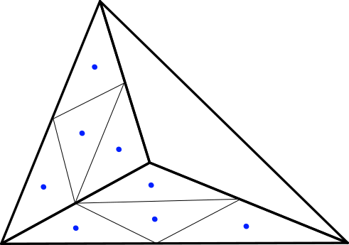
Figure 1: An example of the subdivision of the tetrahedron $T$, with two faces explicitly subdivided for $k=2$, where the blue dots are the baricenters of the triangles obtained with the subdivision.

Lemma 3.6.

Let $T\subset\mathbb{R}^{3}$ be a $3$-simplex and $\mathcal{F}$ a finite union of planes in $\mathbb{R}^{3}$. Let $A\in\mathbb{R}^{N\times 3}$ and assume that $A=\sum_{j=1}^{M}b^{j}\otimes t^{j}$, with $b^{j}\in\mathcal{Q}$, $t^{j}\in\mathbb{S}^{2}$. Then there exist sequences of polyhedral measures $\mu_{k},\nu_{k},\omega_{k},\rho_{k}\in\mathcal{M}^{1}_{{\rm loc}}(\mathbb{R}^{3};\mathcal{Q}\times\mathbb{S}^{2})$ such that $\mu_{k}=\nu_{k}+\omega_{k}+\rho_{k}$ and satisfy the following:

1. $$\nu_{k}=\frac{1}{k^{4}}\sum_{j=1}^{M}b^{j}\otimes t^{j}\mathcal{H}^{1}\mathbin{\vrule height=6.88889pt,depth=0.0pt,width=0.55974pt\vrule height=0.55974pt,depth=0.0pt,width=5.59721pt}(\Gamma^{j}_{k}\cap T^{k}),$$

   where $\Gamma^{j}_{k}$ are straight lines parallel to $t^{j}$, satisfying

   $$\frac{1}{k^{4}}\mathcal{H}^{1}\mathbin{\vrule height=6.88889pt,depth=0.0pt,width=0.55974pt\vrule height=0.55974pt,depth=0.0pt,width=5.59721pt}\Gamma^{j}_{k}\overset{\ast}{\rightharpoonup}\mathcal{L}^{3},$$ (3.6)

   and $T_{k}\subset\subset T$ is a tetrahedron satisfying ${\rm dist}(T_{k},\partial T)\leq{\rm diam}(T)/k^{2}$;

2. $\mu_{k}\mathbin{\vrule height=6.88889pt,depth=0.0pt,width=0.55974pt\vrule height=0.55974pt,depth=0.0pt,width=5.59721pt}T=\nu_{k}+\omega_{k}$, $\mu_{k}\mathbin{\vrule height=6.88889pt,depth=0.0pt,width=0.55974pt\vrule height=0.55974pt,depth=0.0pt,width=5.59721pt}T^{c}=\rho_{k}$, $\|\mu_{k}\|(\partial T)=0$, $\mathcal{H}^{1}(\operatorname{supp}\rho_{k}\cap\mathcal{F})=0$;

3. for every compact set $K\subset\mathbb{R}^{3}$ it holds $\lim_{k\to+\infty}\|\omega_{k}\|(K)+\|\rho_{k}\|(K)=0$;

4. for every $\varphi\in[C_{c}(\mathbb{R}^{3})]^{N\times 3}$ it holds

   $$\lim_{k\rightarrow\infty}\int_{T}\varphi d\mu_{k}=\int_{T}\langle\varphi,A\rangle dx;$$

5. for every $\varphi\in[C_{c}^{\infty}(\mathbb{R}^{3})]^{N}$ it holds

   $$\langle\mu_{k},\nabla\varphi\rangle=\sum_{h=1}^{4k^{2}}\langle An_{h},\varphi(d(T,k,h))\rangle\mathcal{H}^{2}(\Delta(k,h)).$$

Proof.

Without loss of generality we may assume that the baricenter of $T$ coincides with the origin and we define $T_{k}:=(1-\frac{1}{k^{2}})T$. Therefore $T_{k}$ is a tetrahedron similar to $T$ and ${\rm dist}(T_{k},\partial T)\leq{\rm diam}(T)/k^{2}$.

The construction is quite natural but somewhat involved, therefore we shall present it in several steps.

Step 1. The segments inside $T_{k}$.

We define the approximating measures inside $T_{k}$. For every $j\in\{1,\ldots,M\}$ we consider the $2$-dimensional vector space $\Pi^{j}$ whose normal is $t^{j}$. Let $v_{1}^{j},v_{2}^{j}$ be an orthonormal base of this plane, and consider the square lattice on $\Pi^{j}$ defined by $\mathcal{G}^{j}_{k}=\operatorname{span}_{\mathbb{Z}}(\frac{1}{k^{2}}v_{1}^{j},\frac{1}{k^{2}}v_{2}^{j})$. We then set $\Gamma_{k}^{j}:=\mathcal{G}^{j}_{k}+\mathbb{R}t^{j}$ and define

$$\nu_{k}^{j}:=\frac{b^{j}}{k^{4}}\otimes t^{j}\mathcal{H}^{1}\mathbin{\vrule height=6.88889pt,depth=0.0pt,width=0.55974pt\vrule height=0.55974pt,depth=0.0pt,width=5.59721pt}\Gamma_{k}^{j}.$$ (3.7)

It is easy to check that $\nu_{k}^{j}\mathbin{\vrule height=6.88889pt,depth=0.0pt,width=0.55974pt\vrule height=0.55974pt,depth=0.0pt,width=5.59721pt}T_{k}\in[\mathcal{M}(\mathbb{R}^{3})]^{N\times 3}$ and that for all $\varphi\in[C_{c}(\mathbb{R}^{3})]^{N\times 3}$ it holds

$$\lim_{k\rightarrow+\infty}\langle\nu_{k}^{j}\mathbin{\vrule height=6.88889pt,depth=0.0pt,width=0.55974pt\vrule height=0.55974pt,depth=0.0pt,width=5.59721pt}T_{k},\varphi\rangle=\lim_{k\rightarrow+\infty}\langle\nu_{k}^{j}\mathbin{\vrule height=6.88889pt,depth=0.0pt,width=0.55974pt\vrule height=0.55974pt,depth=0.0pt,width=5.59721pt}T,\varphi\rangle =\langle b^{j}\otimes t^{j}\mathcal{L}^{3}\mathbin{\vrule height=6.88889pt,depth=0.0pt,width=0.55974pt\vrule height=0.55974pt,depth=0.0pt,width=5.59721pt}T,\varphi\rangle.$$ (3.8)

The measure inside $T_{k}$ is then

$$\nu_{k}:=\sum_{j=1}^{M}\nu_{k}^{j}\mathbin{\vrule height=6.88889pt,depth=0.0pt,width=0.55974pt\vrule height=0.55974pt,depth=0.0pt,width=5.59721pt}T_{k},$$ (3.9)

which then converges weakly$*$ to $A\,\mathcal{L}^{3}\mathbin{\vrule height=6.88889pt,depth=0.0pt,width=0.55974pt\vrule height=0.55974pt,depth=0.0pt,width=5.59721pt}T$.

We now subdivide $\partial T$ in triangles that we call ${\Delta(h,k)}$, for $h=1,\cdots,4k^{2}$ as specified in (3.4), i.e., $\partial T=\bigcup_{h=1}^{4k^{2}}\Delta(k,h)$ and $d(T,k,h)$ is the baricenter of $\Delta(k,h)$. This subdivision induces in turns a subdivision of $\partial T_{k}$ in triangles $\delta(h,k)=(1-\frac{1}{k^{2}})\Delta(h,k)$ by projecting from the origin the $\Delta(k,h)$ onto $\partial T_{k}$. Hence we can write $\partial T_{k}=\bigcup_{h=1}^{4k^{2}}\delta(k,h)$ with $|x-y|\less C\operatorname{diam}(T)k^{-1}$ for every $x\in\Delta(h,k),y\in\delta(k,h)$.

Up to removing a negligible number of lines (so that (3.8) still holds), we can assume that $\Gamma^{j}_{k}$ intersects $\partial T_{k}$ only on isolated points and that none of these points belong to more than one triangle $\delta(k,h)$. Indeed for each one of the $4k^{2}$ triangles $\delta(k,h)$ there are at most $\mathcal{O}(k)$ lines that intersect its contour, hence there are at most $\mathcal{O}(k^{3})$ lines that ought to be discarded but each line has a mass of $\mathcal{O}(k^{-4})$, hence the total error is negligible in the limit. We can also assume that $\mathcal{H}^{1}(\Gamma_{k}^{j}\cap\Gamma_{k}^{i})=0$ for every $j\not=i$.

Step 2. Definition in $T\smallsetminus T_{k}$

For each $1\leq h\leq 4k^{2}$ we now want to connect the lines of $\nu_{k}$, which end on $\delta(k,h)$, with the baricenter of $\Delta(k,h)$. We define

$$R(k,j,h):=\Gamma_{k}^{j}\cap\delta(k,h),\qquad N(k,j,h):=\#R(k,j,h).$$ (3.10)

We observe that $\mathcal{H}^{2}(\delta(k,h))=(1-\frac{1}{k^{2}})^{2}\mathcal{H}^{2}(\Delta(k,h))$ and hence

$$\begin{split}&|\mathcal{H}^{2}(\Delta(k,h))-\mathcal{H}^{2}(\delta(k,h))|\leq C\frac{(\operatorname{diam}(T))^{2}}{k^{4}},\\ &N(k,j,h)\leq Ck^{4}\mathcal{H}^{2}(\delta(k,h))\leq C(\operatorname{diam}(T))^{2}k^{2}.\end{split}$$ (3.11)

In order to concentrate the mass in the baricenter $d(T,k,h)$ of each $\Delta(k,h)$ we connect each point $p\in R(k,j,h)$ to $d(T,k,h)$ using a small straight segment $[p,d(T,k,h)]$. On each of these segments we then define the measure

$$\omega(k,j,h,p):=\frac{1}{k^{4}}b^{j}\otimes t_{p}\mathcal{H}^{1}\mathbin{\vrule height=6.88889pt,depth=0.0pt,width=0.55974pt\vrule height=0.55974pt,depth=0.0pt,width=5.59721pt}[p,d(T,k,h)],$$ (3.12)

where $t_{p}$ is the unit tangent vector in the direction $(d(T,k,h)-p)\operatorname{sign}(\langle t_{j},n_{h}\rangle)$ and $n_{h}$ is the outward normal vector of $\delta(k,h)$.

We then define

$$\omega_{k}:=\sum_{j=1}^{M}\sum_{h=1}^{4k^{2}}\sum_{p\in R(k,j,h)}\omega(k,j,h,p).$$ (3.13)

Since $\|\omega(k,j,h,p)\|(T)\leq C\operatorname{diam}(T)|b^{j}|k^{-5}$ from (3.11) we infer

$$\|\omega_{k}\|(\mathbb{R}^{n})\leq C\frac{1}{k}(\operatorname{diam}(T))^{3}\sum_{j=1}^{M}|b^{j}|,$$ (3.14)

and then

$$\lim_{k\rightarrow+\infty}\|\omega_{k}\|(\mathbb{R}^{n})=0.$$ (3.15)

Figure 2: A portion of $\mu_{k}$, for a single $j$ and in a two dimensional schematization. The blue dots are the baricenter of the $\Delta(k,h)^{\prime}s$.

See Figure 2 for a representation of a portion of $\nu^{j}_{k}$ and $\omega(k,j,h,p)$.

Step 3. Definition outside $T$.
We define the mass at the baricenter $d(T,k,h)$ to be the following vector valued quantity:

$$B(T,k,h):=\sum_{j=1}^{M}N(k,j,h)\operatorname{sign}(\langle t^{j},n_{h}\rangle)\frac{b^{j}}{k^{4}}.$$ (3.16)

This definition makes sense: indeed we observe that $\operatorname{supp}(\nu_{k}+\omega_{k})$ is given by a finite family of piecewise straight lines connecting different baricenters, hence using Remark 2.1 one can show that for every $\varphi\in[C_{c}^{1}(\mathbb{R}^{3})]^{N}$ it holds

$$\langle\nu_{k}+\omega_{k},\nabla\varphi\rangle=\sum_{h=1}^{4k^{2}}\langle B(T,k,h),\varphi(d(T,k,h))\rangle,$$ (3.17)

which means precisely that the vector valued mass carried by $\nu_{k}+\omega_{k}$ at each baricenter on $\partial T$ is given by $B(T,k,h)$.

For every $\Delta(k,h)$ with $1\leq h\leq 4k^{2}$ we define the measures

$$\rho_{k}(h):=(\mathcal{H}^{2}(\Delta(k,h))An_{h}-B(T,k,h))\otimes\tau(k,h)\mathcal{H}^{1}\mathbin{\vrule height=6.88889pt,depth=0.0pt,width=0.55974pt\vrule height=0.55974pt,depth=0.0pt,width=5.59721pt}\gamma(k,h),$$ (3.18)

where $\gamma(k,h)$ is an arbitrary half line with direction $\tau(k,h)$, not intersecting $\mathcal{F}$ and having endpoint in $d(T,k,h)$ (see Remark 3.9 for the heuristics).
Again recalling Remark 2.1, for every $\varphi\in[C_{c}^{\infty}(\mathbb{R}^{3})]^{N}$ it holds

$$\langle\rho_{k}(h),\nabla\varphi\rangle=\langle\mathcal{H}^{2}(\Delta(k,h))An_{h}-B(T,k,h),\varphi(d(T,k,h))\rangle.$$ (3.19)

We then define the total average error as follows

$$\rho_{k}:=\sum_{h=1}^{4k^{2}}\rho_{k}(h).$$ (3.20)

We now want to show that, for every compact set $K$, $\|\rho_{k}\|(K)$ tends to zero. With that aim in mind we first prove the following claim.

Claim: there exists a universal constant $C$ such that

$$|B(T,k,h)-\mathcal{H}^{2}(\delta(k,h))An_{h}|\leq C\frac{1}{k^{3}}\operatorname{diam}(T)\sum_{j=1}^{M}|b_{j}|.$$ (3.21)

From the definition of $B(T,k,h)$ and from the fact that $An_{h}=\sum_{j=1}^{M}b_{j}\langle t_{j},n_{h}\rangle$ it is clear that we only need to consider $1\leq h\leq 4k^{2}$ and $1\leq j\leq M$ such that $\langle t^{j},n_{h}\rangle\not=0$. Let then $j,h$ be as above and consider the elementary cell of the lattice $\mathcal{G}_{k}^{j}$, i.e., $\mathcal{C}_{k}^{j}:=\Pi_{j}\cap\{\frac{s_{1}}{k^{2}}v_{1}^{j}+\frac{s_{2}}{k^{2}}v_{2}^{j}\,:\,0\leq s_{1},s_{2}\leq 1\}$. Let also $\Sigma_{h}$ be the plane that contains $\delta(k,h)$, then if we denote by $P^{h,j}_{k}$ the elementary cell of the (planar) lattice $\Sigma_{h}\cap\Gamma^{j}_{k}$ we have that

$$\mathcal{H}^{2}(P^{h,j}_{k})=\mathcal{H}^{2}(\mathcal{C}_{k}^{j})\dfrac{1}{|\langle t^{j},n_{h}\rangle|}=\frac{1}{k^{4}|\langle t^{j},n_{h}\rangle|},$$ (3.22)

since $\mathcal{C}_{k}^{j}$ is obtained by orthogonal projection of a translation of $P^{h,j}_{k}$ on $\Pi_{j}$.
From the previous equality and the fact that $A=\sum_{j=1}^{M}b_{j}\otimes t_{j}$ we obtain that

$$\mathcal{H}^{2}(\delta(k,h))An_{h}=\sum_{j=1}^{M}\dfrac{\mathcal{H}^{2}(\delta(k,h))}{\mathcal{H}^{2}(P^{h,j}_{k})}\operatorname{sign}(\langle t^{j},n_{h}\rangle)\frac{b^{j}}{k^{4}}.$$ (3.23)

Therefore in order to show (3.21), in view of the definition of $B(T,k,h)$, it is enough to show that

$$\left|\dfrac{\mathcal{H}^{2}(\delta(k,h))}{\mathcal{H}^{2}(P^{h,j}_{k})}-N(k,h,j)\right|\leq C\operatorname{diam}(T)k.$$ (3.24)

This inequality clearly holds true, since $\mathcal{H}^{2}(\delta(k,h))/\mathcal{H}^{2}(P^{h,j}_{k})$ counts the number of points in $R(k,h,j)$ up to an error due to those points of the lattice $\Sigma_{h}\cap\Gamma^{j}_{k}$ that are close to the contour of $\delta(k,h)$. The number of such points can in turn be estimated by $C\operatorname{diam}(T)k$, which proves (3.24).

Finally from (3.21), (3.11) and (3.20) we obtain that for every compact set $K\subset\mathbb{R}^{n}$ we have

$$\|\rho_{k}\|(K)\leq\sum_{h=1}^{4k^{2}}\|\rho_{k}(h)\|(K)\leq\frac{C}{k}\operatorname{diam}(T){\rm diam}(K)\sum_{j=1}^{M}|b_{j}|,$$ (3.25)

which then tends to zero as $k\to+\infty$.

Step 4. Conclusions.

We now combine all these constructions and define $\mu_{k}$ in the whole of $\mathbb{R}^{n}$, namely

$$\mu_{k}:=\nu_{k}+\omega_{k}+\rho_{k}.$$ (3.26)

We claim that $\mu_{k}$ satisfies the thesis. Indeed (i) follows directly from the definition of $\nu_{k}$ in Step 1, while (ii) from the definition of $\omega_{k}$ and $\rho_{k}$ in Step 2 and Step 3 respectively. Property (iii) follows from (3.14) and (3.25). As for (iv) it is a consequence of (3.8), (ii) and (iii).

To see (v) we simply write $\langle\mu_{k},\nabla\varphi\rangle=\langle\nu_{k}+\omega_{k},\nabla\varphi\rangle+\langle\rho_{k},\nabla\varphi\rangle$ and recall (3.17) and (3.19).

∎

Remark 3.7.

We observe that each of the approximating measures $\mu_{k}$ constructed in the previous lemma are such that

$$\|\mu_{k}\|(K)\leq C\left[\mathcal{L}^{3}(T)+\frac{1}{k}\operatorname{diam}(T){\rm diam}(K)+\frac{1}{k}(\operatorname{diam}(T))^{3}\right]\sum_{j=1}^{M}|b_{j}|,$$ (3.27)

for every compact set $K\subset\mathbb{R}^{3}$.

Remark 3.8.

Let $A(x)=\sum_{i=1}^{M}A_{i}\chi_{T^{i}}(x)$ be a piecewise constant function with null divergence, where $A_{i}\in\mathbb{R}^{N\times 3}$ and the $T^{i}$’s are tetrahedra. If $T^{i}$ and $T^{j}$ share a face, then, by integrating over a small cube across the common face, it is easy to see that it must hold

$$A_{i}\nu=A_{j}\nu,$$ (3.28)

where $\nu$ is the unit normal vector of the common face.

Remark 3.9.

A few comments on the measures constructed in Lemma 3.6 are in order. Recall the definition of $\Gamma^{j}_{k}$ and $\delta(k,h)$ given in Lemma 3.6. With a direct computation one can see that, on average, the number of lines in $\Gamma^{j}_{k}$ intersecting $\delta(k,h)$ is $\hat{N}(k,j,h):=\mathcal{H}^{2}(\delta(k,h))k^{4}|\langle t^{j},n_{h}\rangle|$. Consequently, given that $A=\sum_{j}b^{j}\otimes t^{j}$, the averaged mass on each baricenter is

$$\hat{B}(T,k,h)=\sum_{j=1}^{M}\hat{N}(k,j,h)\operatorname{sign}(\langle t^{j},n_{h}\rangle)\frac{b^{j}}{k^{4}}=\mathcal{H}^{2}(\delta(k,h))An_{h}.$$

Furthermore, since (3.28) holds, it is clear how the averaged mass is a more convenient boundary datum than the exact mass $B(T,k,h)$, as defined in (3.16). Indeed, in Lemma 3.10, the averaged mass will allow us to glue together the local construction of Lemma 3.6 performed in different tetrahedra preserving the divergence free constraint.

In this sense, the $\rho_{k}$’s in (3.26) are to be considered just a small correction necessary to pass from $B$ to $\hat{B}$.

We now glue together the local construction of Lemma 3.6 to obtain the global approximating sequence.

Lemma 3.10.

Let $\Omega\subset\mathbb{R}^{3}$ be an open set, $\mathcal{T}=\{T^{1},\cdots,T^{M}\}$ be an admissible triangulaiton of $\Omega$ and $A=\sum_{i=1}^{M}A_{i}\chi_{T^{i}}$ be a divergence free piecewise constant function, with respect to $\mathcal{T}$, where $A_{i}\in\mathbb{R}^{N\times 3}$. Assume that $A_{i}=\sum_{j=1}^{M^{i}}b_{j}^{i}\otimes t_{j}^{i}$, for some $b_{j}^{i}\in\mathcal{Q}$, $t_{j}^{i}\in\mathbb{S}^{2}$, then there exists a sequence of polyhedral measures $\mu_{k}\in\mathcal{M}_{df}^{1}(\Omega;\mathcal{Q}\times\mathbb{S}^{2})$ such that

1. $\mu_{k}\overset{\ast}{\rightharpoonup}\operatorname{A}\mathcal{L}^{3}\mathbin{\vrule height=6.88889pt,depth=0.0pt,width=0.55974pt\vrule height=0.55974pt,depth=0.0pt,width=5.59721pt}\Omega$,

2. there exists a sequence of measures $\eta_{k}\in\mathcal{M}^{1}(\Omega;\mathcal{Q}\times\mathbb{S}^{2})$ such that $\|\eta_{k}\|(K)\to 0$, for every compact set $K$, and

   $$\mu_{k}=\frac{1}{k^{4}}\sum_{i=1}^{M}\sum_{j=1}^{M^{i}}b_{j}^{i}\otimes t_{j}^{i}\mathcal{H}^{1}\mathbin{\vrule height=6.88889pt,depth=0.0pt,width=0.55974pt\vrule height=0.55974pt,depth=0.0pt,width=5.59721pt}(\Gamma^{j,i}_{k}\cap T^{i}_{k})+\eta_{k},$$ (3.29)

   where $T^{i}_{k}\subset\subset T^{i}$ with ${\rm dist}(T^{i}_{k},\partial T^{i})\leq{\rm diam}(T^{i})/k^{2}$, and $\Gamma_{k}^{j,i}$ is a union of straight lines parallel to $t^{i}_{j}$. Furthermore $\mathcal{H}^{1}(\operatorname{supp}(\mu_{k})\cap\partial T^{i})=0$ for every $1\leq i\leq M$.

Proof.

For every tetrahedron $T^{i}\in\mathcal{T}$ we apply Lemma 3.6 on $A_{i}$ to find four sequences of measures $\mu_{k}^{i},\nu_{k}^{i},\omega^{i}_{k},\rho^{i}_{k}\in\mathcal{M}^{1}_{{\rm loc}}(\mathbb{R}^{3};\mathcal{Q}\times\mathbb{S}^{2})$. Define $\mu_{k}:=\sum_{i=1}^{M}\mu_{k}^{i}$ and $\eta_{k}:=\sum_{i=1}^{M}\omega_{k}^{i}+\rho^{i}_{k}$. Set $\Omega^{\prime}:={\rm int}(\cup_{T^{i}\in\mathcal{T}}T^{i})$.

We observe that from (ii) of Lemma 3.6 , by taking an appropriate family of plane $\mathcal{F}$ (containing all the boundaries $\partial T^{i}$), without loss of generality we can assume that $\mathcal{H}^{1}(\operatorname{supp}\mu_{k}^{i}\cap\operatorname{supp}\mu_{k}^{l})=0$ for $i\not=l$, and $\mathcal{H}^{1}(\operatorname{supp}(\mu_{k})\cap\partial T^{i})=0$ for every $1\leq i\leq M$. In particular $\mu_{k}\in\mathcal{M}^{1}(\Omega;\mathcal{Q}\times\mathbb{S}^{2})$ since each $\mu_{k}^{i}$ does and they have disjoint support.

We first show that, with this definition, $\mu_{k}$ is divergence free in $\Omega^{\prime}$. Indeed from (v) of Lemma 3.6 we get that for every $\varphi\in[C^{\infty}_{c}(\Omega^{\prime})]^{N}$

$$\langle\mu_{k},\nabla\varphi\rangle=\sum_{i=1}^{M}\langle\mu_{k}^{i},\nabla\varphi\rangle=\sum_{i=1}^{M}\sum_{h=1}^{4k^{2}}\langle\mathcal{H}^{2}(\Delta_{i}(k,h))A_{i}n^{i}_{h},\varphi(d(T_{i},k,h))\rangle,$$

where $n_{h}^{i}$ is the outer unit normal with respect to $T_{i}$, and $\Delta_{i}(k,h)$ is one of the $4k^{2}$ triangles that tile $\partial T_{i}$ (as defined in (3.4)). Then using that for any pair $i,j\in\{1,\ldots,M\}$ and $h,h^{\prime}\in\{1,\ldots,4k^{2}\}$ we have that either $\mathcal{H}^{2}(\Delta_{i}(k,h)\cap\Delta_{j}(k,h^{\prime}))=0$ or $\Delta_{i}(k,h)=\Delta_{j}(k,h^{\prime})$ we denote the set

$$\mathcal{A}_{k}=\{(i,j,h,h^{\prime}):\ i<j\,,\ \mathcal{H}^{2}(\Delta_{i}(k,h)\cap\Delta_{j}(k,h^{\prime}))>0\},$$

and we can rewrite

$$\langle\mu_{k},\nabla\varphi\rangle=\sum_{\mathcal{A}_{k}}\langle\mathcal{H}^{2}(\Delta_{i}(k,h))(A_{i}n^{i}_{h}+A_{j}n_{h^{\prime}}^{j}),\varphi(d(T_{i},k,h))\rangle=0,$$ (3.30)

since $n_{h}^{i}=-n_{h^{\prime}}^{j}$ and (3.28) holds.

Furthermore, from (iv) of Lemma 3.6 and the fact that $\lim_{k}\|\mu_{k}^{i}\|(\operatorname{int}T^{i})=\lim_{k}\|\mu_{k}^{i}\|(\Omega)$, we have that $\mu_{k}\overset{\ast}{\rightharpoonup}A\mathcal{L}^{n}$ in $\Omega$.

Finally property (ii) is a direct consequence of choice of $\mathcal{F}$, the definition of $\mu_{k}^{i}$ and $\rho_{k}^{i}$, and (i) of Lemma 3.6. ∎

Proof of Theorem 3.5.

Let $\mu\in[\mathcal{M}(\Omega)]^{N\times 3}$ be divergence free. From Theorem 3.2 we obtain a sequence $\mathcal{T}_{k}=\{T_{k}^{i}\}_{i=1,\cdots,M(k)}$ of admissible triangulations of $\Omega$ and a sequence $A_{k}:\Omega\to\mathbb{R}^{N\times 3}$ of piecewise constant functions relatively to $\mathcal{T}_{k}$, such that $A_{k}\mathcal{L}^{3}\mathbin{\vrule height=6.88889pt,depth=0.0pt,width=0.55974pt\vrule height=0.55974pt,depth=0.0pt,width=5.59721pt}\Omega$ approximates strictly $\mu$. For each $k$, let $A_{k}(\Omega)=\{A_{k}^{i}\}_{i=1,\cdots,M(k)},$ and write $A_{k}^{i}=\sum(A_{k}^{i})_{lm}e_{l}\otimes e_{m}$. From Lemma 3.10 applied to each $A_{k}$ we then get a sequence of measures $\mu_{k}^{h}\in\mathcal{M}_{df}^{1}(\Omega;\mathcal{Q}\times\mathbb{S}^{2})$ approximating $A_{k}\mathcal{L}^{3}\mathbin{\vrule height=6.88889pt,depth=0.0pt,width=0.55974pt\vrule height=0.55974pt,depth=0.0pt,width=5.59721pt}\Omega$ and such that, recalling (3.27), $\|\mu_{k}^{h}\|(\Omega)\leq C\|A_{k}\|_{L^{1}}\leq C\|\mu\|(\Omega)$, hence we can find a diagonal sequence $\mu_{k}^{h(k)}\overset{\ast}{\rightharpoonup}\mu$. ∎

4 The upper bound

The approximation results proved above provide a local construction which is the crucial ingredient for the proof of the upper bound, which is stated and proved below.

Proposition 4.1.

Let $\psi:\mathbb{Z}\times\mathbb{S}^{2}\longrightarrow[0,+\infty)$ be $\mathcal{H}^{1}$-elliptic and obey $\frac{1}{c}|b|\leq\psi(b,t)$ for all $b\in\mathbb{Z}$ and $t\in\mathbb{S}^{2}$. Let $\Omega\subset\mathbb{R}^{3}$ be a bounded open set, simply connected with Lipschitz boundary. Then for every $\mu\in[\mathcal{M}(\Omega)]^{N\times 3}$ with null divergence there exists a sequence $\mu_{\sigma}\in\mathcal{M}_{df}^{1}(\Omega;\sigma\mathbb{Z}^{N}\times\mathbb{S}^{2})$ converging weakly$*$ to $\mu$ such that

$$\liminf_{\sigma\to 0}E_{\sigma}(\mu_{\sigma})\leq E_{0}(\mu).$$

Proof.

The strategy of the proof follows closely the one in [8]. It consists of a first step in which, using the approximation results, one reduces to divergence free measures concentrated on polyhedral curves whose limiting energy resolves the convexification procedure in the definition of the $\Gamma$-limit. With this we reduce the analysis to the construction of a recovery sequence for the auxiliary functional $F_{\infty}$ defined as follows:

$$F_{\infty}(\mu,\omega):=\begin{cases}\displaystyle{\int_{\Gamma\cap\omega}\psi_{\infty}(\theta,t)d\mathcal{H}^{1}}\ \ &\hbox{if }\mu=\theta\otimes t\mathcal{H}^{1}\mathbin{\vrule height=6.88889pt,depth=0.0pt,width=0.55974pt\vrule height=0.55974pt,depth=0.0pt,width=5.59721pt}\Gamma\in\mathcal{M}_{df}^{1}(\omega;\mathcal{Q}\times\mathbb{S}^{2}),\\ &\mu\hbox{ polyhedral};\\ +\infty&\hbox{otherwise},\end{cases}$$ (4.1)

where $\omega$ is an open set, and $F_{\infty}(\mu):=F_{\infty}(\mu,\Omega)$.

Step 1: Reduction from $E_{0}$ to $F_{\infty}$.

We now prove that $E_{0}$ is the relaxation of $F_{\infty}$ with respect to the weak$*$ topology, i.e., $E_{0}=\bar{F}_{\infty}$. Note that from the definition of $E_{0}$ we have that $E_{0}\leq F_{\infty}$, and hence $E_{0}\leq\bar{F}_{\infty}$, therefore we just have to prove the upper bound. From Theorem 3.2 and Reshetnyak Continuity Theorem we obtain that divergence free piecewise constant measures are dense in energy for $E_{0}$, i.e., for every divergence free measure $\mu\in[\mathcal{M}(\Omega)]^{N\times 3}$ there exists a sequence of divergence free piecewise constant measures $\nu_{k}$ such that $\nu_{k}\overset{\ast}{\rightharpoonup}\mu$ and

$$\lim_{k\rightarrow+\infty}E_{0}(\nu_{k})=E_{0}(\mu).$$ (4.2)

Thus, since the weak$*$ convergence is metrizable on bounded set of $\mathcal{M}(\Omega)$, without loss of generality we can now assume $\mu$ to be a divergence free piecewise constant measure of the form

$$\mu=\sum_{i=1}^{M}\chi_{T^{i}}A_{i}\mathcal{L}^{3},$$ (4.3)

where $\mathcal{T}=\{T^{1},\cdots,T^{M}\}$ is an admissible triangulation of $\Omega$. We thus construct the recovery sequence in the relaxation of $F_{\infty}$ for a measure $\mu$ as in (4.3).

First recall that $g$ is the convex envelope of $g_{\infty}$. Moreover we know (see Lemma 2.4) that $g$ is finite and that $\psi_{\infty}(b,t)=+\infty$ if and only if $b\in\mathbb{R}^{N}\smallsetminus\mathcal{Q}$. Therefore for any fixed $\varepsilon>0$ and for every matrix $A_{i}$, with $i\in\{1,\ldots,M\}$, we find $M^{i}_{\varepsilon}\leq 3N+1$ rank one matrices of the form $\tilde{b}^{j,i}_{\varepsilon}\otimes t^{j,i}_{\varepsilon}$, with $\tilde{b}^{j,i}_{\varepsilon}\in\mathcal{Q}$, $t^{j,i}_{\varepsilon}\in\mathbb{S}^{2}$, and coefficients $\lambda^{j,i}_{\varepsilon}>0$ such that $\sum_{j=1}^{M^{i}_{\varepsilon}}\lambda^{j,i}_{\varepsilon}=1$, $\sum_{j=1}^{M^{i}_{\varepsilon}}\lambda^{j,i}_{\varepsilon}\tilde{b}^{j,i}_{\varepsilon}\otimes t^{j}_{\varepsilon}=A_{i}$, and

$$g(A_{i})+\varepsilon\geq\sum_{j=1}^{M^{i}_{\varepsilon}}\lambda^{j,i}_{\varepsilon}\psi_{\infty}(\tilde{b}^{j,i}_{\varepsilon},t^{j,i}_{\varepsilon})=\sum_{j=1}^{M^{i}_{\varepsilon}}\psi_{\infty}(\lambda^{j,i}_{\varepsilon}\tilde{b}^{j,i}_{\varepsilon},t^{j,i}_{\varepsilon}),$$ (4.4)

Setting $b^{j}_{\varepsilon}:=\lambda^{j}_{\varepsilon}\tilde{b_{\varepsilon}}^{j}\in\mathcal{Q}$ we then have

$$(g(A_{i})+\varepsilon)\mathcal{L}^{3}(T^{i}\cap\Omega)\geq\sum_{j=1}^{M^{i}_{\varepsilon}}\psi_{\infty}(b^{j,i}_{\varepsilon},t^{j,i}_{\varepsilon})\mathcal{L}^{3}(T^{i}\cap\Omega).$$ (4.5)

We now apply Lemma 3.10 to $\mu=\sum_{i=1}^{M}\chi_{T^{i}}A_{i}$, with $A_{i}=\sum_{j=1}^{M_{\varepsilon}^{i}}b^{j,i}_{\varepsilon}\otimes t^{j,i}_{\varepsilon}$ satisfying (4.4), to find a sequence of measures $\mu_{k}^{\varepsilon}\in\mathcal{M}_{df}^{1}(\Omega;\mathcal{Q}\times\mathbb{S}^{2})$ converging to $\mu$, and $\eta_{k}^{\varepsilon}$ vanishing as $k\to+\infty$.

On the other hand, from (ii) of Lemma 3.6 and using that $\psi_{\infty}(\theta,t)\leq C|\theta|$ for all $\theta\in\mathcal{Q}$ it is easy to see that $F_{\infty}(\mu_{k}^{\varepsilon},\operatorname{int}(T^{i})\cap\Omega)<+\infty$ and

$$F_{\infty}(\mu_{k}^{\varepsilon},\operatorname{int}(T^{i})\cap\Omega)\leq\sum_{j=1}^{M^{i}_{\varepsilon}}\psi_{\infty}(b^{j,i}_{\varepsilon},t^{j,i}_{\varepsilon})\frac{1}{k^{4}}\mathcal{H}^{1}(T_{k}^{i}\cap\Omega\cap\Gamma^{j,i,\varepsilon}_{k})+C\|\eta_{k}^{\varepsilon}\|(T^{i}\cap\Omega).$$ (4.6)

Hence from (3.6) of Lemma 3.6 we get

$$\limsup_{k\rightarrow+\infty}F_{\infty}(\mu_{k}^{\varepsilon},\operatorname{int}(T^{i})\cap\Omega)\leq\sum_{j=1}^{M^{i}_{\varepsilon}}\psi_{\infty}(b^{j,i}_{\varepsilon},t^{j,i}_{\varepsilon})\mathcal{L}^{3}(T^{i}\cap\Omega).$$ (4.7)

Recalling (4.5) we then get

$$E_{0}(\mu)+\varepsilon\mathcal{L}^{3}(\Omega) =\sum_{i=1}^{M}(g(A_{i})+\varepsilon)\mathcal{L}^{3}(T^{i}\cap\Omega)\geq\sum_{i=1}^{M}\limsup_{k\rightarrow\infty}F_{\infty}(\mu_{k}^{\varepsilon},\operatorname{int}(T^{i})\cap\Omega)$$

$$\geq\limsup_{k\rightarrow\infty}\sum_{i=1}^{M}F_{\infty}(\mu_{k}^{\varepsilon},\operatorname{int}(T^{i})\cap\Omega)=\limsup_{k\rightarrow\infty}F_{\infty}(\mu^{\varepsilon}_{k},\Omega),$$

where in the last line we used the fact that $\mathcal{H}^{1}(\operatorname{supp}(\mu_{k})\cap\partial T^{i})=0$ for all $i$.

Now (iii) of Proposition 2.3 implies $\psi_{\infty}(b,t)\geq c|b|$ for $b\in\mathcal{Q}$, hence, from estimate (4.4) we deduce the existence of a universal constant $C>0$ such that

$$\sum_{j=1}^{N_{\varepsilon}}|b_{\varepsilon}^{j,i}|\leq C(|A_{i}|+\varepsilon).$$ (4.8)

In particular, given (3.27), we have that the family of measures $\mu^{\varepsilon}_{k}$ is uniformly bounded. Therefore, since the weak$*$ topology is metrizable on bounded set, via a diagonal argument we infer that for every divergence free measure $\mu\in[\mathcal{M}(\Omega)]^{N\times 3}$ there exists a sequence $\tilde{\mu}_{h}$ weakly$*$ converging to $\mu$, such that

$$\limsup_{h\to+\infty}F_{\infty}(\tilde{\mu}_{h})\leq E_{0}(\mu).$$ (4.9)

In particular this sequence satisfies $F_{\infty}(\tilde{\mu}_{h})<+\infty$.

Step 2: Recovery sequence for $F_{\infty}$.

We now prove that for a given $\tilde{\mu}=\theta\otimes t\mathcal{H}^{1}\mathbin{\vrule height=6.88889pt,depth=0.0pt,width=0.55974pt\vrule height=0.55974pt,depth=0.0pt,width=5.59721pt}\Gamma\in\mathcal{M}_{df}^{1}(\Omega;\mathbb{R}^{N}\times\mathbb{S}^{2})$, with $\Gamma$ polyhedral we can construct a sequence $\hat{\mu}_{\sigma}\in\mathcal{M}_{df}^{1}(\Omega;\sigma\mathbb{Z}^{N}\times\mathbb{S}^{2})$ converging to $\tilde{\mu}$ and such that

$$\limsup_{\sigma\rightarrow 0}E_{\sigma}(\hat{\mu}_{\sigma})=F_{\infty}(\tilde{\mu}).$$ (4.10)

Without loss of generality we can assume $F_{\infty}(\tilde{\mu})<+\infty$. First we observe that, since $\Gamma$ is composed by a finite number of straight segments and $\tilde{\mu}$ is divergence free, $\theta$ must be constant on each segment. In particular $\theta\in\mathcal{Q}$ attains a finite number of values. Therefore we can apply Theorem $2.5$ of [6] to $\mu$, deducing that there exists a finite number of polyhedral closed loops $\Gamma_{i}$ with constant Burgers vector $\theta_{i}$ such that

$$\tilde{\mu}=\sum_{i}\theta_{i}\otimes t_{i}\mathcal{H}^{1}\mathbin{\vrule height=6.88889pt,depth=0.0pt,width=0.55974pt\vrule height=0.55974pt,depth=0.0pt,width=5.59721pt}\Gamma_{i}.$$

Here the $\theta_{i}$ do not necessary belong to $\sigma\mathbb{Z}^{N}$. Therefore we define the following approximation of $\tilde{\mu}$ with measures

$$\hat{\mu}_{\sigma}:=\sum_{i}\sigma\left\lfloor\dfrac{\theta_{i}}{\sigma}\right\rfloor\otimes t_{i}\mathcal{H}^{1}\mathbin{\vrule height=6.88889pt,depth=0.0pt,width=0.55974pt\vrule height=0.55974pt,depth=0.0pt,width=5.59721pt}\Gamma_{i}\in\mathcal{M}_{df}^{1}(\Omega;\sigma\mathbb{Z}^{N}\times\mathbb{S}^{2}),$$ (4.11)

where we denote $\left\lfloor\frac{b}{\sigma}\right\rfloor=(\big{\lfloor}\frac{b_{1}}{\sigma}\big{\rfloor},\cdots,\big{\lfloor}\frac{b_{N}}{\sigma}\big{\rfloor})$. These measures have the same support of $\mu$, and satisfy $E_{\sigma}(\hat{\mu}_{\sigma})<+\infty$. We observe that $\hat{\mu}_{\sigma}$ is a finite sum of closed loops with constant multiplicity, therefore, again by Theorem $2.5$ in [6], it is divergence free.

Since $\sigma\left\lfloor\frac{\theta_{i}}{\sigma}\right\rfloor$ converges to $\theta_{i}$, we have that $\hat{\mu}_{\sigma}\overset{\ast}{\rightharpoonup}\tilde{\mu}$. Let now consider an arbitrary sequence $\sigma_{j}$ converging to $0$, then

$$E_{\sigma_{j}}(\hat{\mu}_{\sigma_{j}})=\int_{\Gamma}\sigma_{j}\psi(z_{j},t)d\mathcal{H}^{1},$$ (4.12)

where $z_{j}(x):=\sum_{i}\left\lfloor\frac{\theta_{i}}{\sigma_{j}}\right\rfloor\chi_{\Gamma_{i}}(x)\in\mathbb{Z}^{N}$. Since, clearly, for $\mathcal{H}^{1}\mathbin{\vrule height=6.88889pt,depth=0.0pt,width=0.55974pt\vrule height=0.55974pt,depth=0.0pt,width=5.59721pt}\Gamma$ a.e. $x$ it holds that $\lim_{j\to+\infty}|z_{j}|=+\infty$ and $\lim_{j\to+\infty}z_{j}/|z_{j}|=\theta/|\theta|$, thanks to (iii) of Lemma 2.3 we deduce

$$\lim_{j\to+\infty}\frac{\psi\left(z_{j},t\right)}{|z_{j}|}=\frac{\psi_{\infty}\left(\theta,t\right)}{|\theta|}.$$

On the other hand clearly it holds that $\lim_{j\to+\infty}\sigma_{j}|z_{j}|=|\theta|$, hence by rewriting

$$\sigma_{j}\psi\left(z_{j},t\right)=\sigma_{j}|z_{j}|\frac{\psi\left(z_{j},t\right)}{|z_{j}|},$$ (4.13)

we deduce that

$$\lim_{j\rightarrow+\infty}\sigma_{j}\psi(z_{j},t)=\psi_{\infty}\left(\theta,t\right),\ \ \ \ \mathcal{H}^{1}\textit{-a.e. }x\in\Gamma.$$ (4.14)

Finally, since $|\sigma_{j}\psi(z_{j},t_{i})|\leq c|\sigma_{j}z_{j}|\leq C(|\theta|+1)$, we conclude via dominated convergence theorem and get

$$\lim_{j\to+\infty}E_{\sigma_{j}}(\hat{\mu}_{\sigma_{j}})=\int_{\Gamma}\psi_{\infty}(\theta,t)d\mathcal{H}^{1}=F_{\infty}(\tilde{\mu}).$$ (4.15)

Step 3: Conclusion

We conclude the proof by combining Step 1 and Step 2. Without loss of generality we can assume that the sequence $\tilde{\mu}_{h}$ constructed in Step 1 satisfies

$$\limsup_{h\to+\infty}F_{\infty}(\tilde{\mu}_{h})=\lim_{h\to+\infty}F_{\infty}(\tilde{\mu}_{h})\leq E_{0}(\mu)<+\infty.$$ (4.16)

Then for every $h$ we obtain via Step 2 a sequence $\hat{\mu}_{\sigma}^{h}$ weakly$*$ converging to $\tilde{\mu}_{h}$ such that

$$\lim_{\sigma\to 0}E_{0}(\hat{\mu}_{\sigma}^{h})=F_{\infty}(\tilde{\mu}_{h}).$$ (4.17)

A further diagonal argument provides the wanted recovery sequence and concludes the proof. ∎

Fundings

The present paper benefits from the support of the PRIN 2017, Variational methods for stationary and evolution problems with singularities and interfaces, 2017BTM7SN-004. Also MF acknowledges the hospitality given by the HIM, Hausdorff Research Institute for Mathematics.
  
Declarations of interest: none.

References

- [1] L. Ambrosio, N. Fusco, and D. Pallara. Functions of bounded variation and free discontinuity problems. Oxford Mathematical Monographs, 2000.
- [2] G. Bellettini, M. Novaga, and M. Paolini. On a crystalline variational problem, part i: first variation and global regularity. Arch. Rational Mech. Anal., 157(3):165–191, 2001.
- [3] J. Bourgain and H. Brezis. New estimates for the Laplacian, the div-curl, and related Hodge systems. Comptes Rendus Mathematique, 338:539–543, 2004.
- [4] F.H. Clarke. Optimization and Nonsmooth Analysis. Canadian Mathematical Society series of monographs and advanced texts. Wiley, 1983.
- [5] S. Conti, A. Garroni, and R. Marziani. Line-tension limits for line singularities and application to the mixed-growth case. arXiv, 2207.01526, 2022.
- [6] S. Conti, A. Garroni, and A. Massaccesi. Modeling of dislocations and relaxation of functionals on 1-currents with discrete multiplicity. Calc. Var. Partial Differential Equations, 54(2):1847–1874, 2015.
- [7] S. Conti, A. Garroni, and S. Müller. Singular kernels, multiscale decomposition of microstructure, and dislocation models. Arch. Rational Mech. Anal., 199:779–819, 2011.
- [8] S. Conti, A. Garroni, and S. Müller. Homogenization of vector-valued partition problems and dislocation cell structures in the plane. Boll. Unione Mat. Ital., 10(1):3–17, 2017.
- [9] S. Conti, A. Garroni, and S. Müller. Dislocation microstructures and strain-gradient plasticity with one active slip plane. J. Mech. Phys. Solids, 93:240–251, 2016. Special Issue in honor of Michael Ortiz.
- [10] S. Conti, A. Garroni, and M. Ortiz. The line-tension approximation as the dilute limit of linear-elastic dislocations. Arch. Rational Mech. Anal., 218:699–755, 2015.
- [11] L. De Luca, A. Garroni, and M. Ponsiglione. -convergence analysis of systems of edge dislocations: the self energy regime. Arch. Rational Mech. Anal., 206:885–910, 2012.
- [12] A. Garroni, G. Leoni, and M. Ponsiglione. Gradient theory for plasticity via homogenization of discrete dislocations. J. Eur. Math. Soc., 12(5):1231–1266, 2010.
- [13] A. Garroni, R. Marziani, and R. Scala. Derivation of a line-tension model for dislocations from a nonlinear three-dimensional energy: The case of quadratic growth. SIAM J. Math. Anal., 53(4):4252–4302, 2021.
- [14] M. Giaquinta, G. Modica, and J. Souček. Cartesian Currents in the Calculus of Variations. Number 37 in Ergebnisse der Mathematik und ihrer Grenzgebiete. 3. Folge/ A Series of Modern Surveys in Mathematics. Springer, Berlin, Heidelberg, 1998.
- [15] J. Goodman, F. Hernandez, and D. Spector. Two approximation results for divergence free vector fields. arXiv, 2010-14079, 2020.
- [16] S. Hofmann, M. Mitrea, and M. E. Taylor. Geometric and transformational properties of Lipschitz domains, Semmes-Kenig-Toro domains, and other classes of finite perimeter domains. J. Geom. Anal., 17:593–647, 2007.
- [17] G. Leoni. A First Course in Sobolev Spaces. American Mathematical Society, second edition, 2017.
- [18] S. Muller, L. Scardia, and C. I. Zeppieri. Geometric rigidity for incompatible fields and an application to strain-gradient plasticity. Indiana Univ. Math. J., 63:1365–1396, 2014.
- [19] M. Ponsiglione. Elastic energy stored in a crystal induced by screw dislocations: From discrete to continuous. SIAM J. Math. Anal., 39(2):449–469, 2007.
- [20] L. Scardia and C. I. Zeppieri. Line-tension model for plasticity as the -limit of a nonlinear dislocation energy. SIAM J. Math. Anal., 44:2372–2400, 2012.
- [21] S. Stanislav. Decomposition of solenoidal vector charges into elementary solenoids, and the structure of normal one-dimensional currents. Algebra i Analiz, 5, no. 4:206–238, 1993. Translation in St. Petersburg Math. J. 5, no. 4, 841–867, 1994.