Reconstructing Turbulent Flows Using Physics-Aware Spatio-Temporal Dynamics and Test-Time Refinement

Abstract.

Accurate simulation of turbulent flows is of crucial importance in many branches of science and engineering. Direct numerical simulation (DNS) provides the highest fidelity means of capturing all intricate physics of turbulent transport. However, the method is computationally expensive because of the wide range of turbulence scales that must be accounted for in such simulations. Large eddy simulation (LES) provides an alternative. In such simulations, the large scales of the flow are resolved and the effects of small scales are modelled. Reconstruction of the DNS field from the low-resolution LES is needed for a wide variety of applications. Thus the construction of super-resolution (SR) methodologies that can provide this reconstruction has become an area of active research. In this work, a new physics-guided neural network is developed for such a reconstruction. The method leverages the partial differential equation that underlies the flow dynamics in the design of spatio-temporal model architecture. A degradation-based refinement method is also developed to enforce physical constraints and to further reduce the accumulated reconstruction errors over long periods. Detailed DNS data on two turbulent flow configurations are used to assess the performance of the model.

1. Introduction

Direct numerical simulation (DNS) of the Navier-Stokes equations is a brute-force computational method and is the method with the highest reliability for capturing turbulence dynamics (Givi, 1994). The computational cost of such simulations is very expensive for flows with high Reynolds numbers. Large eddy simulation (LES) is a popular alternative, concentrating on the larger scale energy-containing eddies, and filtering the small scales of transport (Sagaut, 2005). In this way, LES can be conducted on coarser grids as compared to DNS, but obviously with less fidelity (Nouri et al., 2017).

Machine learning, including super-resolution (SR) methods (Park et al., 2003), have been advocated as a means of reconstructing highly resolved DNS from LES data. These methods have shown tremendous success in reconstructing high-resolution data in various commercial applications. The majority of current SR models use convolutional network layers (CNNs)  (Albawi et al., 2017) to extract representative spatial features and transform them through complex non-linear mappings to recover high-resolution images. Starting from the end-to-end convolutional SRCNN model (Dong et al., 2014), several investigators have explored the addition of other structural components such as skip-connections (Zhang et al., 2018a, b; Ahn et al., 2018; Van Duong et al., 2021; Dai et al., 2019; Van Duong et al., 2021), channel attention (Zhang et al., 2018a), adding adversarial training objectives (Ledig et al., 2017; Chen et al., 2018; Wang et al., 2018a, b; Karras et al., 2017; Upadhyay and Awate, 2019; Cheng et al., 2021; Wenlong et al., 2021), and more recently, Transformer (Parmar et al., 2018)-based SR methods  (Fang et al., 2022b; Yang et al., 2020; Lu et al., 2022; Fang et al., 2022a; Wang et al., 2022; Zou et al., 2022; Liang et al., 2022).

Given their success in computer vision, SR methods are becoming increasingly popular in turbulence reconstruction (Liu et al., 2020; Xie et al., 2018; Deng et al., 2019; Wang et al., 2018b; Fukami et al., 2019, 2021). Despite their popularity, these methods face some limitations when it comes to representing continuous flow dynamics in the spatial and temporal fields using discrete data samples. Consequently, they can learn spurious patterns between sparse observations, which often lack generalizability. Additionally, the training of SR models is hindered by the scarcity of high-fidelity DNS data due to the required high computational cost of such simulations.

In this work, a novel method termed the “continuous networks using differential equations” (CNDE) is developed to improve the SR reconstruction. This development is by leveraging the underlying physical relationships to guide the learning of generalizable spatial and temporal patterns in the reconstruction process. The method consists of three components: the Runge-Kutta transition unit (RKTU), the temporally-enhancing layer (TEL), and degradation-based refinement. The RKTU structure is designed based on the governing partial differential equations (PDEs) and is used for capturing continuous spatial and temporal dynamics of turbulent flows. The TEL structure is designed based on the long-short-term memory (LSTM) (Hochreiter and Schmidhuber, 1997) model and is responsible for capturing long-term temporal dependencies. The degradation-based refinement is to adjust the reconstructed data by enforcing consistency with physical constraints.

Model appraisal is made by considering detailed data sets pertaining to two turbulent flow configurations: (1) a forced isotropic turbulent (FIT) flow (Minping et al., 2012), and (2) the Taylor-Green vortex (TGV) flow (Brachet et al., 1984). The results of the consistency assessments demonstrate the capability of the CNDE in terms of the reconstruction performance over space and time. The effectiveness of each component of the methodology is demonstrated qualitatively and quantitatively.

2. Related Work

2.1. Super-Resolution

Single image super-resolution (SISR) via deep learning has been the subject of many investigations in computer vision. These methods derive their power primarily from the utilization of convolutional network layers (Albawi et al., 2017), which extract spatial texture features and transform them through complex non-linear mappings to recover high-resolution data. One of the earliest SR methods for SISR is SRCNN (Dong et al., 2014), which learns an end-to-end mapping between coarse-resolution and high-resolution images by employing a series of convolutional layers. Another scheme is the skip-connection layers (Van Duong et al., 2021; Dai et al., 2019; Zhang et al., 2018b; Ahn et al., 2018; Tai et al., 2017), which enable the bypassing of abundant low-frequency information and emphasize the relevant information to improve the stability of the optimization process in deep neural networks. Several investigators have explored the adversarial training objective by using the generative adversarial network (GAN) for SISR. For example, the SRGAN model (Ledig et al., 2017) stacks the deep residual network to build a deeper generative network for image super-resolution and also introduces a discriminator network to distinguish between reconstructed images and real images using an adversarial loss function. The ultimate goal is to train the generative network in a way that the reconstructed images cannot be easily distinguished by the discriminator. One major advantage of SRGAN is that the discriminator can help extract representative features from high-resolution data and enforce such features in the reconstructed images. Several variants of SRGAN are given in Refs. (Chen et al., 2018; Wang et al., 2018a, b; Karras et al., 2017; Upadhyay and Awate, 2019; Cheng et al., 2021; Wenlong et al., 2021).

The Transformer (Vaswani et al., 2017) has revolutionized natural language processing (NLP) by introducing self-attention mechanisms, allowing it to efficiently process long-range dependencies in the sequences of data. This method can effectively capture contextual information from the entire input sequence, leading to significant advancements in various NLP tasks like machine translation, sentiment analysis and etc. The Transformer has also been introduced into the SISR problem (Parmar et al., 2018; Fang et al., 2022b; Yang et al., 2020; Lu et al., 2022; Fang et al., 2022a; Wang et al., 2022; Zou et al., 2022; Liang et al., 2022). For example, Yang et al. (Yang et al., 2020) developed the TTSR model, which uses a learnable texture extractor to extract textures from low-resolution (LR) images and reference high-resolution (HR) images in order to recover target HR images. Lu et al. (Lu et al., 2022) developed the ESRT model, which optimizes the original Transformer to achieve competitive reconstruction performance with low computational cost.

2.2. Super-Resolution for Turbulent Flows

There is a significant interest in developing SR techniques for high-resolution flow reconstructions. Fukami et al. (Fukami et al., 2019, 2021; Liu et al., 2020) created an improved CNN-based hybrid DSC/MS model to explore multiple scales of turbulence and capture the spatio-temporal turbulence dynamics. Liu et al. (Liu et al., 2020) developed another CNN-based model MTPC to simultaneously include spatial and temporal information to fully capture features in different time ranges. Xie et al. (Xie et al., 2018) introduced tempoGAN, which augments a GAN model with an additional discriminator network along with new loss functions that preserve temporal coherence in the generation of physics-based simulations of fluid flow. Deng et al. (Deng et al., 2019) demonstrated that both SRGAN and ESRGAN (Wang et al., 2018b) can produce good reconstructions. Yang et al. (Yang et al., 2023) created an FSR model based on a back-projection network to achieve 3D reconstruction. Xu et al. (Xu et al., 2023) introduced a Transformer-based SR method to build the SRTT model for capturing small-scale details of turbulent flow.

2.3. Physics-Guided Machine Learning

Recent studies have shown promise in integrating physics into machine learning models for improved predictive performance (Willard et al., 2022). These methods typically enforce physics in the loss function (He et al., 2023; Hanson et al., 2020; Daw et al., 2022; Jia et al., 2019; Read et al., 2019; Chen et al., 2021) or use simulated data for pre-training and augmentation (Jia et al., 2023; Chen et al., 2023; He et al., 2023; Chen et al., 2022; Liu et al., 2022). Hanson et al. (Hanson et al., 2020) introduced ecological principles as physical constraints into the loss function to improve the lake surface water phosphorus prediction. Karpatne et al. (Daw et al., 2022) developed a hybrid machine learning and physics model to guarantee that the density of water at a lower depth is always greater than the density at any depth above. Jia et al. (Jia et al., 2019) and Read et al. (Read et al., 2019) extended this idea by including an additional penalty for the violation of the energy conservation law. In the flow data reconstruction, Chen et al. (Chen et al., 2021) constructed a PGSRN method to enforce zero divergences of the velocity field in incompressible flows. Despite the promise of these methods, they may lead to slow convergence in optimization and performance degradation, especially when the physical relationships are complex or have uncertain parameters.

A means of imposing the physics is by considering the partial differential equations (PDEs) that govern the physical phenomena. In some cases, however, direct integration of the governing PDEs using standard numerical methods  (Wikipedia contributors, 2022a) can become prohibitively expensive. An alternative is to solve PDEs via neural operators (Li et al., 2020; Equer et al., 2023; Boussif et al., 2022). For example, Li et al. (Li et al., 2020) introduced the Fourier neural operator (FNO) to model PDEs for learning the mappings between infinite-dimensional spaces of functions using the integral operator. The integral operator of this approach is restricted to convolution and instantiated through a linear transformation in the Fourier domain. However, the major limitation of neural operators for flow data reconstruction lies in their lack of explicit knowledge about the specific form of the underlying PDE (Naiver-Stoke equation). Neural operators directly learn the relation between input data and outputs without incorporating the intrinsic structure and physics encoded in the PDE. This can lead to inefficiencies and challenges in effectively capturing complex flow dynamics. An alternative direction is to embed the physics equations or relationships in the modeling structure (Khandelwal et al., 2020; Muralidhar et al., 2020; Bao et al., 2022). One such example is the encoding of the Navier-Stokes equation in a recurrent unit, as demonstrated in our previous work (Bao et al., 2022). However, this method may accumulate errors in long-term predictions, and it does not consider the use of LES data in reconstructing DNS data within the recurrent unit.

3. Problem Under Investigation

In this work, the transport of unsteady, three-dimensional turbulent flows is the subject of main consideration. In all cases, the flow is assumed to be Newtonian and incompressible with a constant density. In the formulation, the space coordinate is identified by the vector ${\bf x}\equiv{x,\ y,\ z}$, and the time is denoted by $t$. The velocity field is denoted by ${\bf V}({\bf x},t)$, with its three components ${u({\bf x},t),\ v({\bf x},t),\ w({\bf x},t)}$ along the three flow directions ${\ x,\ y,\ z}$, respectively. The pressure, the density, and the dynamic viscosity are denoted by $p({\bf x},t)$, $\rho({\bf x},t)$, and $\nu$, respectively. The latter two are assumed constant. The (dummy) parameters $\textbf{Q}({\bf x},t)$ (as a vector), and/or $Q$ (as a scalar) are used to denote a transport variable.

All of the flows considered are statistically homogeneous. High-resolution DNS and lower-resolution LES data are considered on $N_{x}\times N_{y}\times N_{z}$, and $M_{x}\times M_{y}\times M_{z}$ grid points, respectively. A box filter  (Jing et al., 2000) is employed to create the LES data from the original DNS. All of the statistical averages, including the Reynolds-averaged values are obtained by data ensembled over the entire domain. In this way, the ensemble averages, denoted by an over-bar are defined by:

(1) $$\overline{\bf{Q}(t)}=\frac{1}{N_{x}\times N_{y}\times N_{z}}\sum_{i}^{N_{x}}\sum_{j}^{N_{y}}\sum_{k}^{N_{z}}{\bf Q}(i,j,k,t),$$

suitable for homogeneous flows. In the training process, the available DNS data is at a regular time interval $\delta$, as $\textbf{Q}^{d}=\{\textbf{Q}^{d}(t)\}$ within the time $\{t_{0},t_{0}+\delta,\ \dots,t_{0}+K\delta\}$. The objective is to predict high-resolution DNS data after the historical data, at time $\{t_{0}+(K+1)\delta,$…$,t_{0}+M\delta\}$. The variable $\textbf{Q}^{l}(x,y,z,t)$ represents the low-resolution LES data at time step $t$. Since the LES data can be created at a lower computational cost, they are used for both training and testing periods and at a higher frequency. The variable $\textbf{Q}^{l}=\{\textbf{Q}^{l}(t)\}$ denotes LES data within the time range $[t_{0},t_{0}+M\delta]$.

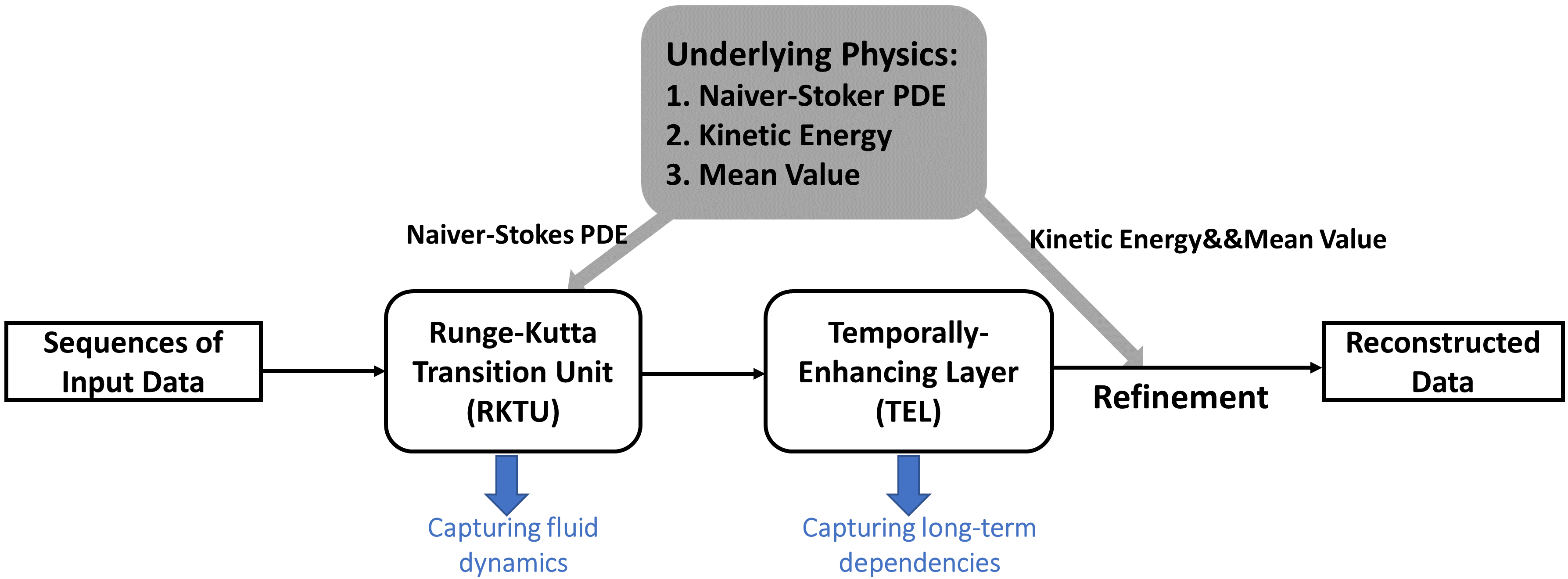
Figure 1. The overall structure of the CNDE method.

The “continuous networks using differential equations” (CNDE) framework consists of two structural components: the Runge-Kutta transition unit (RKTU), and the temporally-enhance layer (TEL). The training is done in two phases: supervised super-resolution training, and degradation-based refinement. These are shown in Fig. 1, and are described in order below.

3.1. Runge-Kutta Transition Unit (RKTU)

The data sets Q pertaining to turbulent flows consist of the transport variables that interact with each other and evolve temporally and spatially. The traditional temporal models, e.g., long-short term memory (LSTM) (Hochreiter and Schmidhuber, 1997), rely on large and consecutive training samples to capture the underlying patterns over time. However, the amount of high-fidelity DNS data is often limited. The RKTU structure is developed for reconstructing flow variables over a long period, given an initial DNS sample $\textbf{Q}^{d}$ at $t$, and frequent low-resolution LES data samples $\textbf{Q}^{l}$. The prediction follows an auto-regressive process in which the predicted DNS $\hat{\textbf{Q}}^{d}(x,y,z,{t})$ at time $t$, and frequent LES data $\textbf{Q}^{l}$ from the current time to the next interval [$t$,$t+\delta$] are used to predict the DNS at next time step $\hat{\textbf{Q}}^{d}(x,y,z,{t+\delta})$.

The RKTU is based on the Runge–Kutta (RK) discretization method (Butcher, 2007). The principal idea is to leverage the continuous physical relationship described by the underlying PDE to bridge the gap between the discrete data samples and the continuous flow dynamics. The scheme can be applied to any dynamical systems governed by deterministic PDEs. Consider the PDE of the target variables Q as expressed by:

(2) $$\textbf{Q}_{t}={\textbf{f}}(t,\textbf{Q};\theta),$$

where $\textbf{Q}_{t}$ denotes the temporal derivative of Q, and ${\textbf{f}}(t,\textbf{Q};\theta)$ is a non-linear function (parameterized by coefficient $\theta$) that summarizes the current value of Q and its spatial variations. The turbulence data follows the Navier-Stokes equation for an incompressible flow. Thus for ${\bf Q}\equiv{\bf V}({\bf x},t)$:

$$\nabla\cdot{\bf Q}=0,$$

(3) $${\textbf{f}(\textbf{Q})}=-\frac{1}{\rho}\nabla p+\nu\Delta\textbf{Q}-(\textbf{Q}\cdot\nabla)\textbf{Q},$$

The term $\nabla$ denotes the gradient operator and $\Delta=\nabla\cdot\nabla$ on each of the components of the velocity. The independent variable $t$ is omitted in the function ${\textbf{f}}(\cdot)$ because ${\textbf{f}}(\textbf{Q})$ in the Navier-Stokes equation is for a specific time $t$ (same with $t$ in $\textbf{Q}_{t}$). Figure 2 shows the overall structure of the method and involves a series of intermediate states $\{\textbf{Q}(t,0),\textbf{Q}(t,1),\textbf{Q}(t,2),\dots,\textbf{Q}(t,N)\}$. The temporal gradients are estimated at these states $\{\textbf{Q}_{t,0},\textbf{Q}_{t,1},\textbf{Q}_{t,2},\dots,\textbf{Q}_{t,N}\}$. Starting from $\textbf{Q}(t,0)=\textbf{Q}(t)$, the RKTU estimates the temporal gradient as $\textbf{Q}_{t,0}$, and then moves $\textbf{Q}(t)$ towards the gradient direction to create the next intermediate state $\textbf{Q}(t,1)$. The process is repeated for $N$ intermediate states. For the fourth-order RK method, as employed here, $N=3$.

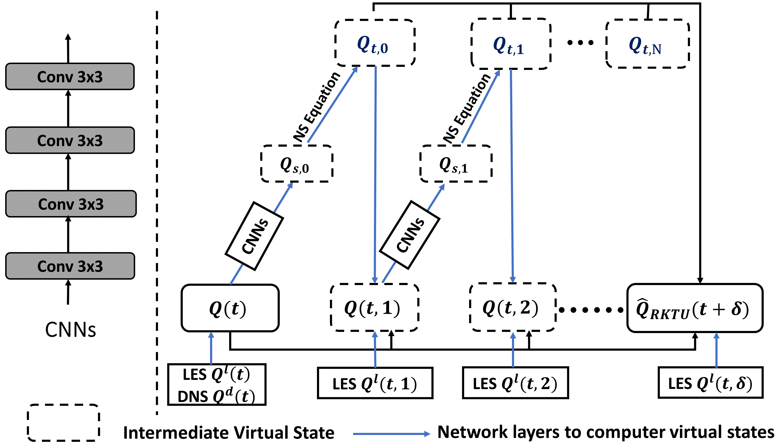
Figure 2. The RKTU based on Naiver Stoke equation for reconstructing turbulent flow data in the spatio-temporal field. $\textbf{Q}_{s,n}$ and $\textbf{Q}_{t,n}$ denote the spatial and temporal derivatives, respectively, at each intermediate time step.

For the starting data point $\textbf{Q}(t)$, an augmentation mechanism is adopted by combining the DNS and LES data: $\textbf{Q}(t)=W^{d}\textbf{Q}^{d}(t)+W^{l}\textbf{Q}^{l}(t)$, where $W^{d}$ and $W^{l}$ are trainable model parameters, and $\textbf{Q}^{l}(t)$ is the up-sampled LES data with the same resolution as DNS. The RKTU estimates the first temporal gradient $\textbf{Q}_{t,0}=\textbf{f}(\textbf{Q}(t))$ using the Navier-Stokes equation and computes the next intermediate state variable $\textbf{Q}(t,1)$ by moving the flow data $\textbf{Q}(t)$ along the direction of temporal derivatives. Given frequent LES data, the intermediate states $\textbf{Q}(t,n)$ are also augmented by using LES data $\textbf{Q}^{l}(t,n)$, as $\textbf{Q}(t,n)=W^{d}\textbf{Q}(t,n)+W^{l}\textbf{Q}^{l}(t,n)$, and they follow the same process to move $\textbf{Q}(t)$ along the estimated gradient $\textbf{Q}_{t,n}$ to compute the next intermediate states $\textbf{Q}(t,n+1)$.

(4) $$\textbf{Q}(t,{1}) =\textbf{Q}(t)+\delta\frac{\textbf{Q}_{t,0}}{2},$$

$$\textbf{Q}(t,{2}) =\textbf{Q}(t)+\delta\frac{\textbf{Q}_{t,1}}{2},$$

$$\textbf{Q}(t,{3}) =\textbf{Q}(t)+\delta\textbf{Q}_{t,2}.$$

The temporal derivative $\textbf{Q}_{t,3}$ is then computed from the last intermediate state by $\textbf{f}(\textbf{Q}(t,{3}))$. According to Eq. (4), the intermediate LES data $\textbf{Q}^{l}(t,n)$ are selected as $\textbf{Q}^{l}(t,1)=\textbf{Q}^{l}(t+\delta/2)$, $\textbf{Q}^{l}(t,2)=\textbf{Q}^{l}(t+\delta/2)$, and $\textbf{Q}^{l}(t,3)=\textbf{Q}^{l}(t+\delta)$. Finally, RKTU combines all the intermediate temporal derivatives as a composite gradient to calculate the final prediction of next step flow data $\hat{\textbf{Q}}_{\text{RKTU}}(t+\delta)$:

(5) $$\hat{\textbf{Q}}_{\text{RKTU}}(t+\delta)=\textbf{Q}(t)+\sum_{n=0}^{N}w_{n}\textbf{Q}_{t,n},$$

where $\{w_{n}\}_{n=1}^{N}$ are the trainable model parameters.

The RKTU requires the temporal derivatives in the Navier-Stokes equation. The RKTU estimates the temporal derivatives through the function ${\textbf{f}}(\cdot)$. According to Eq. (3), the evaluation of ${\textbf{f}}(\cdot)$ requires explicitly estimation of the first-order and second-order spatial derivatives. One of the most popular approaches for evaluating spatial derivatives is through finite difference methods (FDMs) (Wikipedia contributors, 2022a). However, the discretization in FDMs can cause larger errors for locations with complex dynamics. The RKTU structure, as depicted in Fig. (2), utilizes convolutional neural network layers (CNNs) to replace the FDMs. The CNNs have the inherent capability to learn additional non-linear relationships from data and capture the spatial derivatives required in the Navier-Stokes equation. After estimating the first-order and second-order spatial derivatives, they are used in Eq. (3) to obtain the temporal derivative $\textbf{Q}_{t,n}$.

The padding strategies for CNNs also need to be considered. Standard padding strategies (e.g., zero padding) do not satisfy the spatial boundary conditions of the flows considered here. These conditions describe how the flow data interact with the external environment. With the assumption of homogeneous turbulence, periodic boundary conditions are imposed on all three flow directions. Thus, periodic data augmentation is made for each of the $6$ faces (of the 3D cubic data) with an additional two layers of data before feeding it to the model.

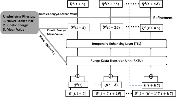
(a) Enhancing Method

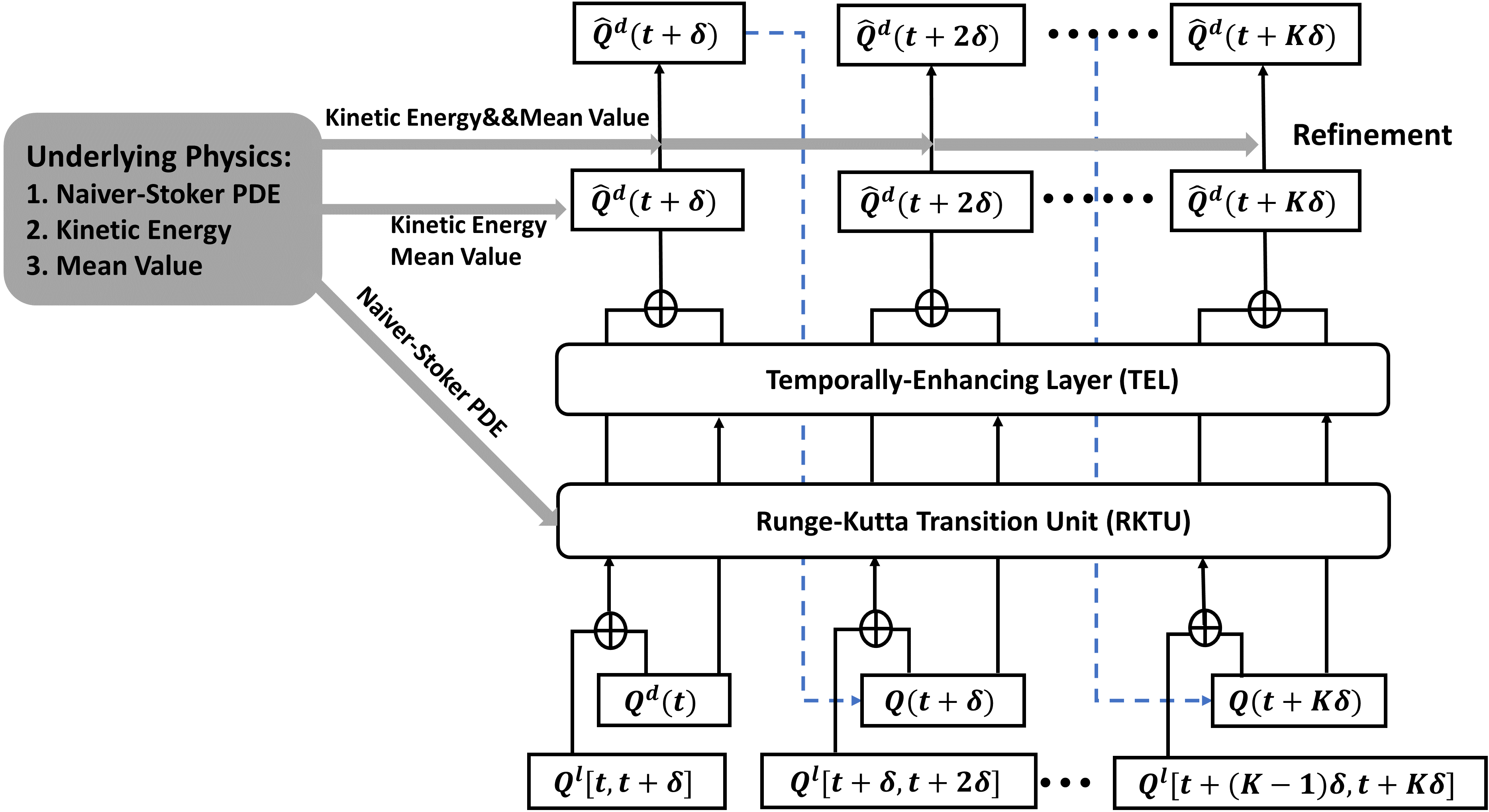
(b) Residual Learning Method

Figure 3. Details of “continuous networks using differential equations” (CNDE) for reconstructing Q. Parts (a) and (b) depict two different approaches to incorporating the TEL component. The solid lines represent the forwarding process in CNDE-based methods. The blue dashed lines represent the reconstructed flow data $\hat{\textbf{Q}}^{d}$ as used as input for the reconstruction of the next time step.

3.2. Temporally-Enhancing Layer (TEL)

The RKTU can capture the data in the spatial and temporal field between a pair of consecutive data points, but it may cause large reconstruction errors in the long-time prediction if the time interval $\delta$ is large. Temporal models, such as long-short-term memory (LSTM) (Hochreiter and Schmidhuber, 1997), and temporal convolutional network (TCN) (Lea et al., 2016) are widely used to capture the long-term dependencies in time series prediction. In this case, the LSTM model is incorporated in a temporally-enhancing layer (TEL) to further enhance the RKTU to capture long-term temporal dependencies. This TEL structure can be replaced by other existing temporal models such as TCN. Figure 3 shows two different approaches for integrating the TEL structure with the RKTU structure. In the first enhancing method shown in Fig. 3 (a), the RKTU output flow data $\hat{\textbf{Q}}_{\text{RKTU}}$ is fed to the TEL structure, which is essentially an LSTM layer. After further processing through the TEL structure, the model produces the reconstructed flow data $\hat{\textbf{Q}}^{\text{d}}(t)$. Given the true DNS data $\textbf{Q}^{d}(t)$ in the training set, the reconstructed loss $\mathcal{L}_{\text{recon}}$ can be expressed using the mean squared error (MSE) loss:

(6) $$\mathcal{L}_{\text{recon}}=\sum_{t}\text{MSE}(\hat{\textbf{Q}}^{d}(t),\textbf{Q}^{d}(t)).$$

The second method uses the TEL structure to complement the output of the RKTU structure, i.e., learning the residual of the RKTU output, as shown in Fig. 3 (b). In the training process, both true DNS data $\textbf{Q}^{d}$ at time $\{t,\dots t+(K-1)\delta\}$ and RKTU output $\hat{\textbf{Q}}_{\text{RKTU}}$ are used to produce the corresponding temporal output feature $\hat{\textbf{Q}}_{\text{TEL}}$ at time $\{t+\delta,\dots,t+K\delta\}$. Then in the testing process, this method uses only the initial true DNS data $\textbf{Q}^{d}$ in time $t+K\delta$ and the next series of predicted DNS data $\hat{\textbf{Q}}^{d}$ as the DNS input to generate $\hat{\textbf{Q}}_{\text{TEL}}$. Finally, this method adopts a linear combination to combine the RKTU output $\hat{\textbf{Q}}_{\text{RKTU}}$ and corresponding TEL output $\hat{\textbf{Q}}_{\text{TEL}}$ to obtain the final reconstructed output $\hat{\textbf{Q}}^{d}$, which can be represented as:

(7) $$\hat{\textbf{Q}}^{d}(t)=w_{r}^{t}\hat{\textbf{Q}}_{\text{RKTU}}(t)+w_{t}^{t}\hat{\textbf{Q}}_{\text{TEL}}(t),$$

where $w_{r}^{t}$ and $w_{t}^{t}$ are trainable parameters. Finally, the reconstructed loss $\mathcal{L}_{\text{recon}}$ can also be represented by Eq. (6).

3.3. Physical Constraints and Refinements

3.3.1. Physical Constraints

For a more accurately reconstructed field, some additional constraints are imposed on the data. Two such constraints are imposed by considering the consistency of (i) the mean velocity field, and (ii) the kinetic energy of turbulence. For (i), the loss function $\mathcal{L}_{\text{mean}}$ between reconstructed data $\hat{\textbf{Q}}^{d}$ and true DNS data $\textbf{Q}^{d}$ is considered:

(8) $$\mathcal{L}_{\text{mean}}=|\overline{\textbf{Q}^{d}}-\overline{\hat{\textbf{Q}}^{d}}|.$$

For (ii), the kinetic energy,], defined as:

(9) $$\mathcal{K}=\frac{1}{2}(u^{2}+v^{2}+w^{2}),$$

is monitored. For this, the loss function is $\mathcal{L}_{\text{kinetic}}$ is:

(10) $$\mathcal{L}_{\text{kinetic}}=|\mathcal{K}(\textbf{Q}^{d})-\mathcal{K}(\hat{\textbf{Q}}^{d})|,$$

where $\mathcal{K}(\textbf{Q}^{d})$ and $\mathcal{K}(\hat{\textbf{Q}}^{d})$ denote the kinetic energy of $\textbf{Q}^{d}$ and $\hat{\textbf{Q}}^{d}$, respectively. The overall loss function $\mathcal{L}$ is:

(11) $$\mathcal{L}=\alpha_{0}\mathcal{L}_{\text{recon}}+\alpha_{1}\mathcal{L}_{\text{mean}}+\alpha_{2}\mathcal{L}_{\text{kinetic}},$$

is considered in which $\alpha_{0}$, $\alpha_{1}$, and $\alpha_{2}$ represent the hyperparameters to control the balance amongst the three constituents.

3.3.2. Degradation-Based Refinement

As shown in Fig. 3, the scheme preserves the physical constraints in the training process and also employs these constraints in the degradation-based test-time refinement process. The objective is to mitigate accumulated errors and structural distortions over long-term prediction by enforcing the physical consistency. The refinement process includes the same set of the loss function: the degradation loss $\mathcal{L}_{\text{deg}}$, the equal-mean loss $\mathcal{L}^{{}^{\prime}}_{\text{mean}}$, and the kinetic energy loss $\mathcal{L}^{{}^{\prime}}_{\text{kinetic}}$ loss. Since it is not possible to access true DNS data during the testing phase, the difference between true DNS $\textbf{Q}^{d}$ and the reconstructed data $\hat{\textbf{Q}}^{d}$ cannot be directly minimized. Thus, in order to protect the overall structure of flow data, a reverse degradation process is employed by using a separate convolutional network, for mapping reconstructed data $\hat{\textbf{Q}}^{d}$ to the corresponding low-resolution LES data $\hat{\textbf{Q}}^{l}$. The loss $\mathcal{L}_{\text{deg}}$ between $\hat{\textbf{Q}}^{l}$ and real LES data $\textbf{Q}^{l}$ is:

(12) $$\mathcal{L}_{\text{deg}}=\text{MSE}(\hat{\textbf{Q}}^{l},\textbf{Q}^{l}).$$

Also, the mean values from the true DNS cannot be used in the equal-mean loss function. Therefore, the corresponding values from the LES data are used as an approximation. As such, the equal-mean loss $\mathcal{L}^{{}^{\prime}}_{\text{mean}}$ between the reconstructed flow data $\hat{\textbf{Q}}^{d}$ and the true LES data $\textbf{Q}^{l}$ can be directly minimized:

(13) $$\mathcal{L}^{{}^{\prime}}_{\text{mean}}=|\overline{\textbf{Q}^{l}}-\overline{\hat{\textbf{Q}}^{d}}|,$$

Similarly, the exact kinetic energy of flow data is not available during the testing period. These values are taken from the DNS in the training data:

(14) $$\mathcal{L^{{}^{\prime}}}_{\text{kinetic}}=|\mathcal{K}(\hat{\textbf{Q}}^{d})-\tilde{\mathcal{K}}|.$$

The final refinement loss function is in the same format $\mathcal{L}{{}^{\prime}}=\alpha_{0}\mathcal{L}_{\text{deg}}+\alpha_{1}\mathcal{L{{}^{\prime}}}_{\text{mean}}+\alpha_{2}\mathcal{L}{{}^{\prime}}_{\text{kinetic}}$. The loss $\mathcal{L}^{{}^{\prime}}$ is adopted to directly adjust the state of reconstructed data for 10 epochs at each test-time time step, and yield an improved reconstruction performance.

4. MODEL APPRAISAL

4.1. Flows Considered

To assess the performance of the proposed methodology, the data sets pertaining to two turbulent flows are considered: a forced isotropic turbulent flow (FIT) (Minping et al., 2012), and the Taylor-Green vortex (TGV)  (Brachet et al., 1984) flow. In both cases, the mean velocity is zero, $\overline{\bf V}(t)=0$, and the Reynolds number is large enough for the flow to exhibit turbulent characteristics.

The FIT data  (Minping et al., 2012) is publicly available from the Johns Hopkins University. This dataset contains the original DNS of forced isotropic turbulence on a $1024\times 1024\times 1024$ collocation points. The flow is forced by injecting energy into the flow at small waver numbers. The DNS data contains $5024$ time steps with time intervals of $0.002$s and includes both the velocity and the pressure fields. The original DNS data are downsampled to $64\times 64\times 64$ grids. The LES data are created on $16\times 16\times 16$ grids. The loss $\mathcal{L}{{}^{\prime}}_{\text{kinetic}}$ is not considered for this flow.

The Taylor-Green vortex (TGV) (Brachet et al., 1984) is an incompressible flow. The evolution of the TGV includes vorticity stretching and the consequent production of small-scale, dissipating eddies. A box flow, with a cubic periodic domain of $[-\pi,\pi]$ (in all three directions) is considered, with the initial conditions:

(15) $$u(x,y,z,0) =\sin(x)\cos(y)\cos(z),$$

$$v(x,y,z,0) =-\cos(x)\sin(y)\cos(z),$$

$$w(x,y,z,0) =0.$$

The LES and DNS resolutions are $32\times 32\times 65$ and $128\times 128\times 65$ respectively. Both LES and DNS data are produced along the $65$ equally-spaced grid points along the $z$ axis.

4.2. Comparative Assessments

Table 1. Reconstruction performance (measured by SSIM, and dissipation difference) on $(u,v,w)$ channels by different methods in the FIT dataset. The performance is measured by the average results of the first 10 time steps.

Method	SSIM	Dissipation Difference
SRCNN	(0.859, 0.851, 0.851)	(0.301, 0.303, 0.303)
RCAN	(0.861, 0.859, 0.859)	(0.299, 0.301, 0.300)
HDRN	(0.861, 0.860, 0.862)	(0.298, 0.298, 0.297)
FSR	(0.861, 0.860, 0.861)	(0.299, 0.297, 0.296)
DCS/MS	(0.861, 0.862, 0.862)	(0.298, 0.295, 0.294)
SRGAN	(0.862, 0.861, 0.863)	(0.296, 0.294, 0.294)
FNO	(0.874, 0.875, 0.874)	(0.265, 0.266, 0.273)
CTN	(0.881, 0.880, 0.881)	(0.253, 0.254, 0.254)
RKTU	(0.898, 0.899, 0.898)	(0.260, 0.261, 0.259)
CNDEp-E	(0.909, 0.909, 0.907)	(0.244, 0.243, 0.245)
CNDEp-R	(0.904, 0.905, 0.905)	(0.249, 0.248, 0.248)
CNDE-E	(0.927, 0.921, 0.922)	(0.193, 0.194, 0.197)
CNDE-R	(0.921, 0.919, 0.920)	(0.196, 0.196, 0.200)

Table 2. Reconstruction performance (measured by SSIM, and dissipation difference) on $(u,v,w)$ channels by different methods in the TGV dataset. The performance is measured by the average results of the first 10 time steps.

Method	SSIM	Dissipation Difference$\times$10
SRCNN	(0.602, 0.603, 0.626)	(0.083, 0.087, 0.079)
RCAN	(0.627, 0.622, 0.631)	(0.073, 0.074, 0.071)
HDRN	(0.638, 0.638, 0.641)	(0.072, 0.072, 0.068)
FSR	(0.646, 0.648, 0.649)	(0.070, 0.073, 0.066)
DSC/MS	(0.647, 0.649, 0.649)	(0.070, 0.071, 0.065)
SRGAN	(0.661, 0.658, 0.666)	(0.068, 0.067,0.058)
FNO	(0.645, 0.646, 0.648)	(0.072, 0.071, 0.072)
CTN	(0.623, 0.624, 0.627)	(0.093, 0.096, 0.087)
RKTU	(0.708, 0.708, 0.688)	(0.049, 0.046, 0.043)
CNDEp-E	(0.724, 0.723, 0.708)	(0.046, 0.041, 0.039)
CNDEp-R	(0.720, 0.719, 0.701)	(0.046, 0.045, 0.040)
CNDE-E	(0.938, 0.918, 0.876)	(0.031, 0.032, 0.026)
CNDE-R	(0.917, 0.909, 0.877)	(0.033, 0.034, 0.028)

4.2.1. CNDE Method and Baselines

The performance of the CNDE method is evaluated and compared with several existing methods for image SR and turbulent flow downscaling. Specifically, the proposed CNDE-based methods, CNDE-E (enhancing-based TEL method) and CNDE-R (residual learning-based TEL method), were implemented. Additionally, four popular SR methods, namely SRCNN (Dong et al., 2014), RCAN (Zhang et al., 2018a), HDRN (Van Duong et al., 2021), SRGAN (Ledig et al., 2017), two popular dynamic fluid downscaling methods, DCS/MS (Fukami et al., 2019) and FSR (Yang et al., 2023), and Fourier neural operator (FNO)(Li et al., 2020), are used as baselines. To better verify the effectiveness of each of the model’s components, four additional baselines are included: convolutional transition network (CTN), RKTU, CNDEp-E, and CNDEp-R. The CTN is created by combining SRCNN and LSTM (Hochreiter and Schmidhuber, 1997). CNDEp-E and CNDEp-R are similar to CNDE-E and CNDE-R, but they are created without using the degradation-based refinement process.

By comparing the CTN with the RKTU, the objective is to demonstrate the advantages of the RKTU in spatio-temporal DNS reconstruction. By comparing the RKTU with the CNDEp-based methods, the goal is to show the effectiveness of introducing the TEL structure. The advantages of the refinement process are demonstrated by comparing the CNDEp-based and CNDE-based methods.

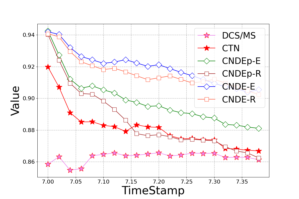
(a) $u$ Channel.

(b) $v$ Channel.

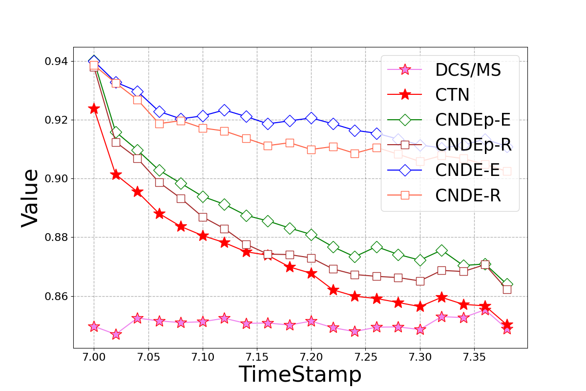
(c) $w$ Channel.

Figure 4. Change of SSIM values produced by different models from 1st (7s) to 20th (7.4s) time step in the FIT dataset.

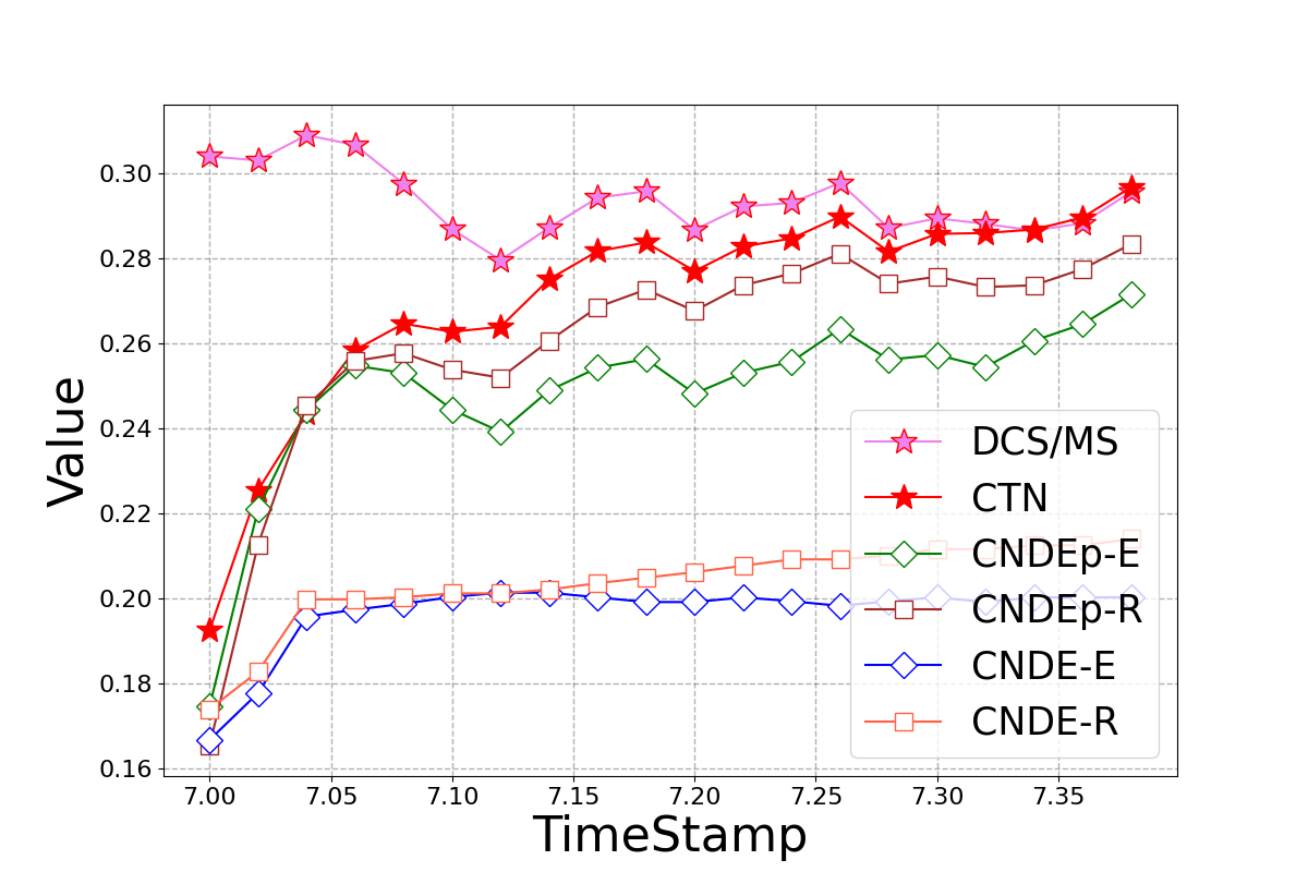
(a) $u$ Channel.

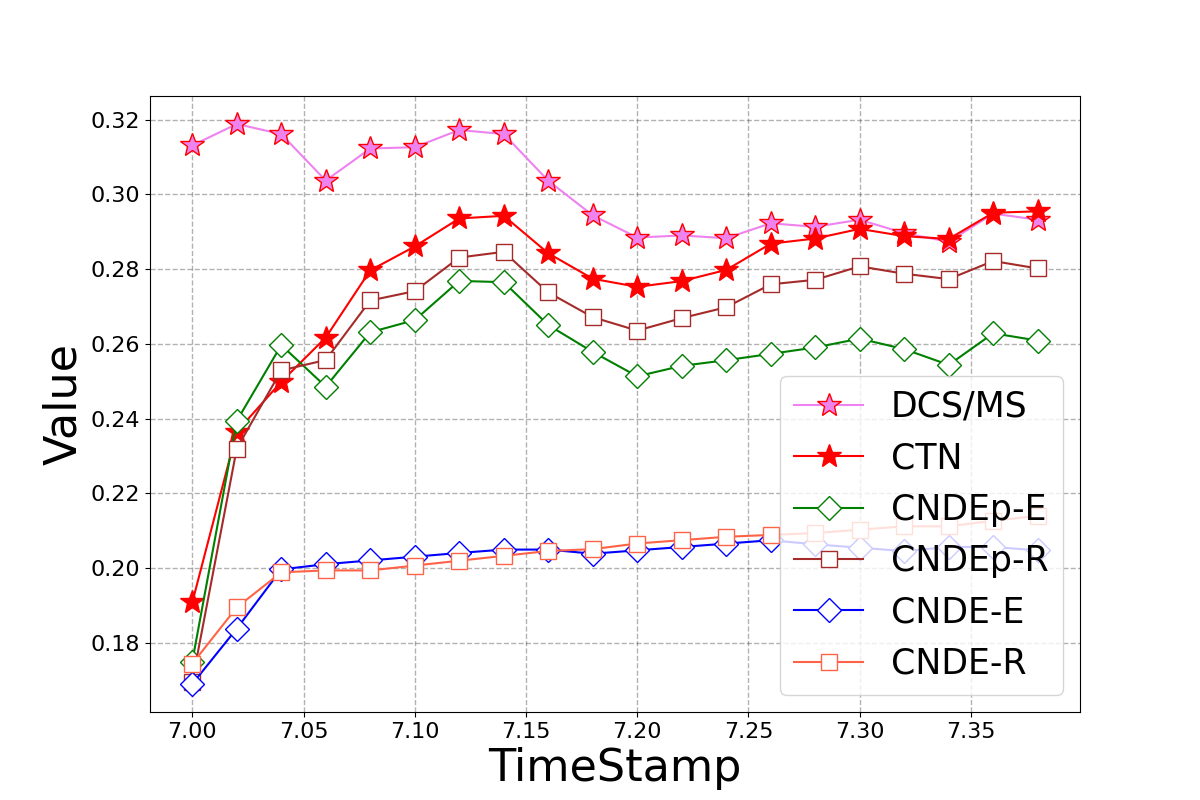
(b) $v$ Channel.

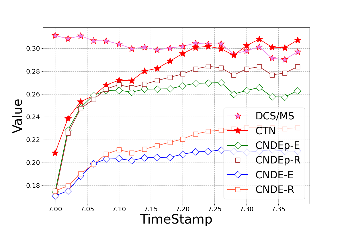
(c) $w$ Channel.

Figure 5. Change of dissipation difference by different models from 1st (7s) to 20th (7.4s) time step in the FIT dataset.

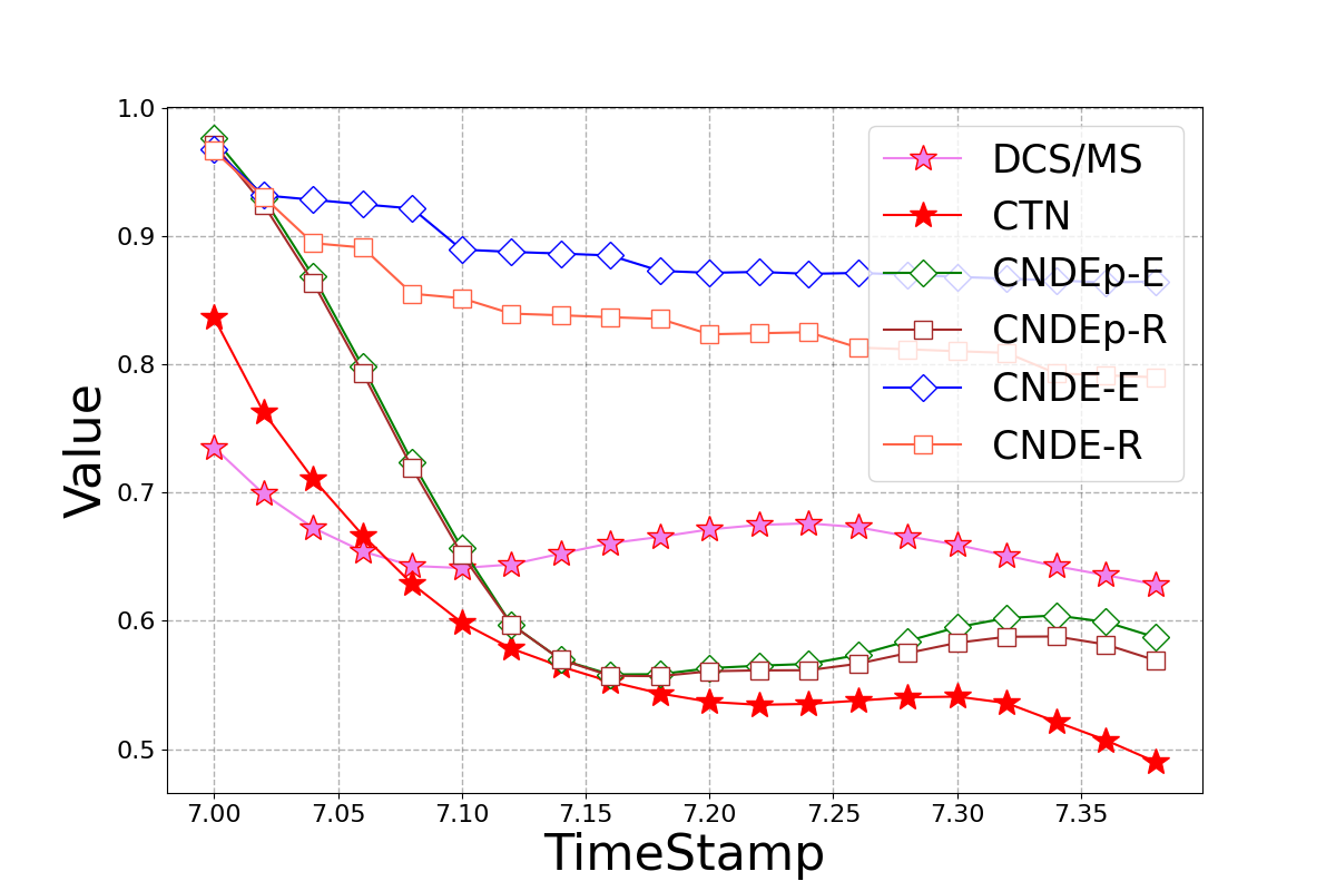
(a) $u$ Channel.

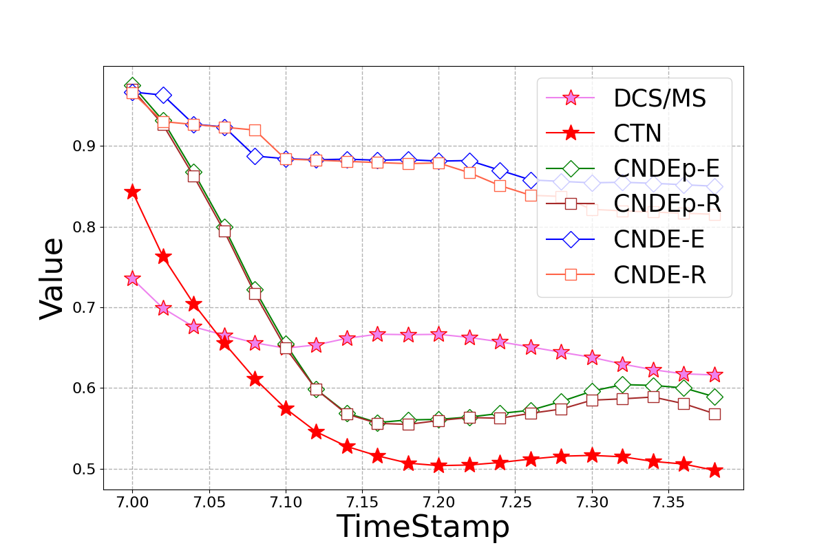
(b) $v$ Channel.

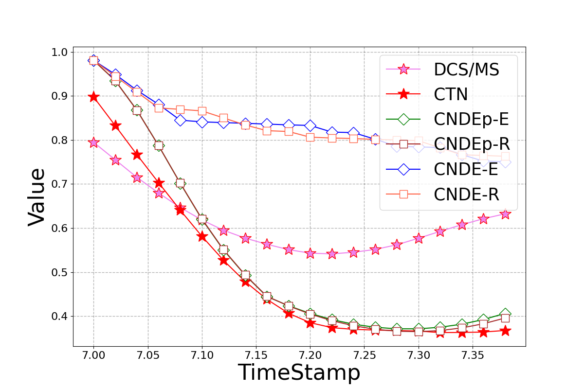
(c) $w$ Channel.

Figure 6. Change of SSIM values produced by different models from 1st (80s) to 20th (120s) time step in the TGV dataset.

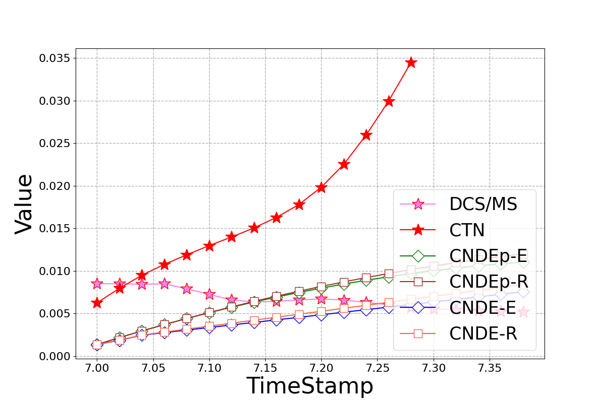
(a) $u$ Channel.

(b) $v$ Channel.

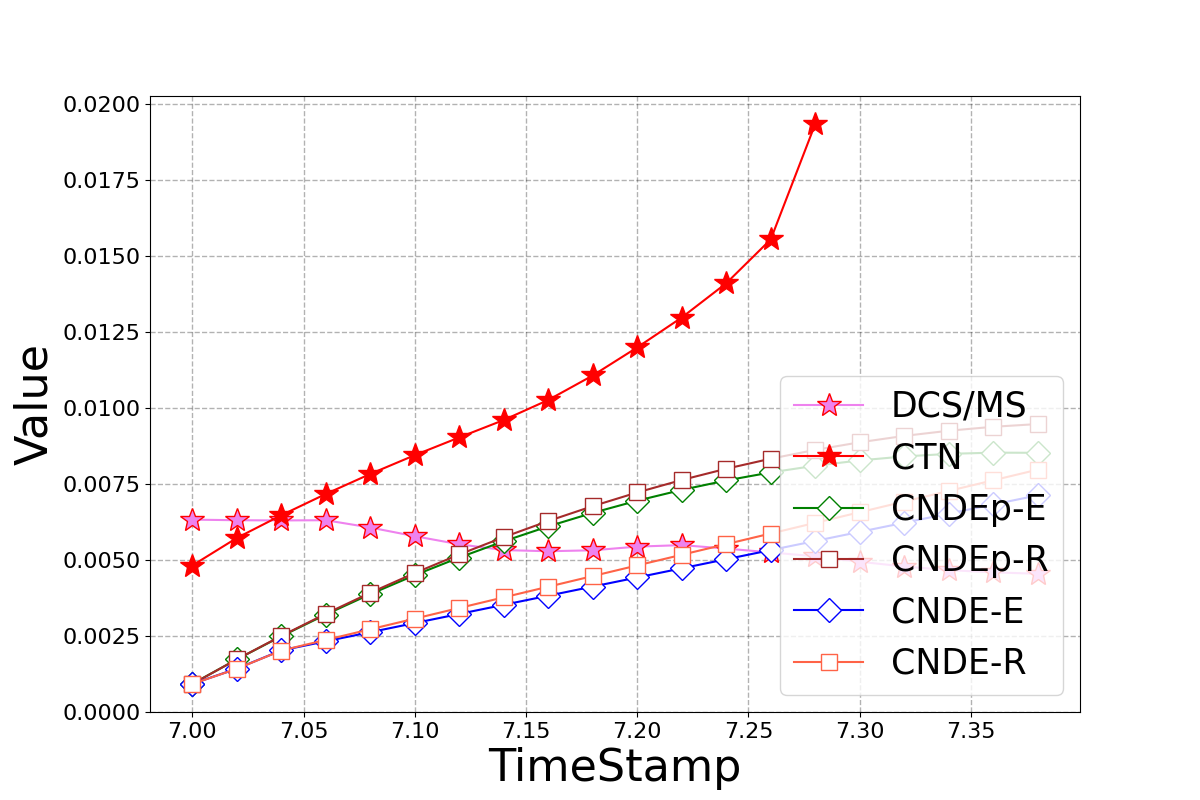
(c) $w$ Channel.

Figure 7. Change of dissipation difference produced by different models from 1st (80s) to 20th (120s) time step in the TGV dataset.

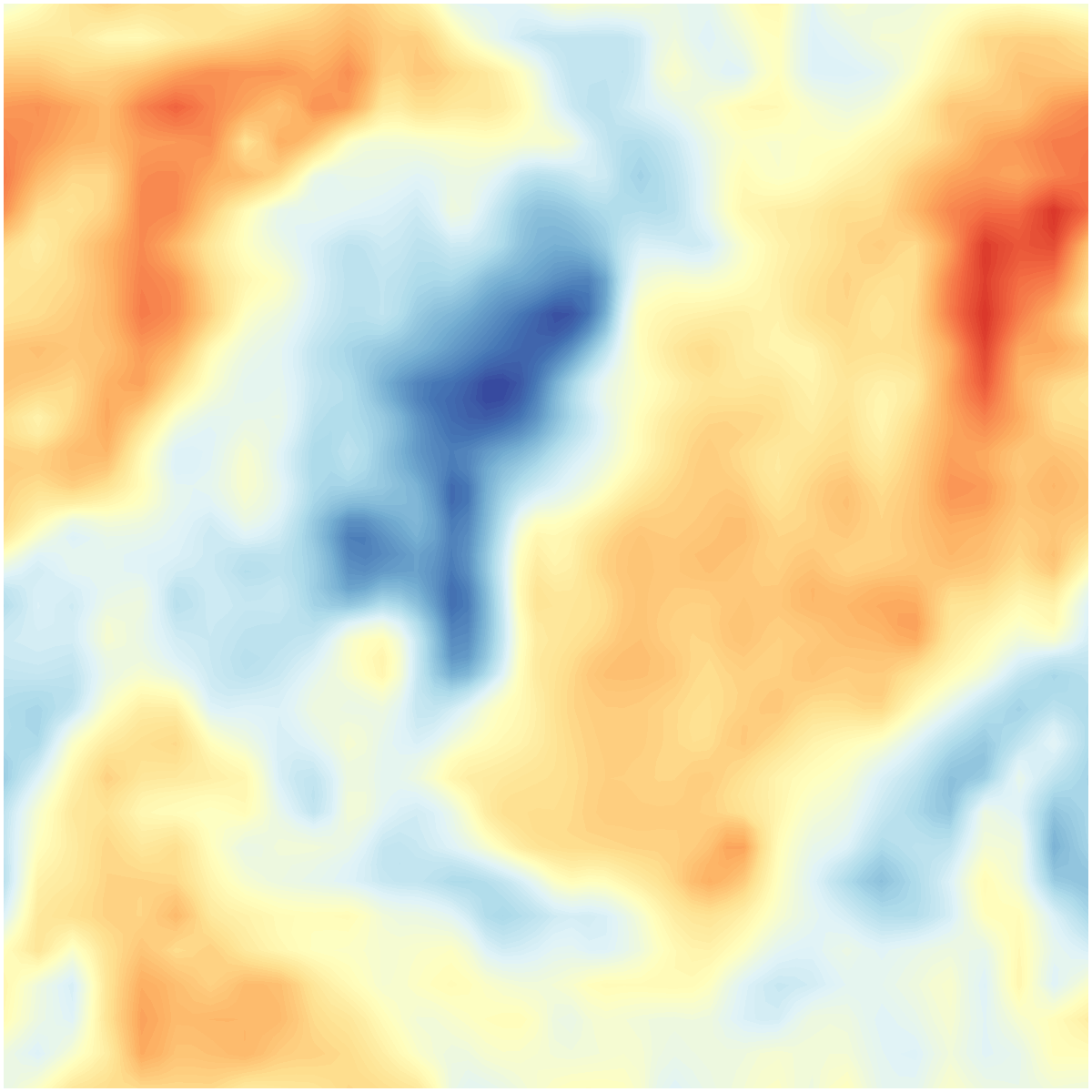
(a) LES Upsampling.

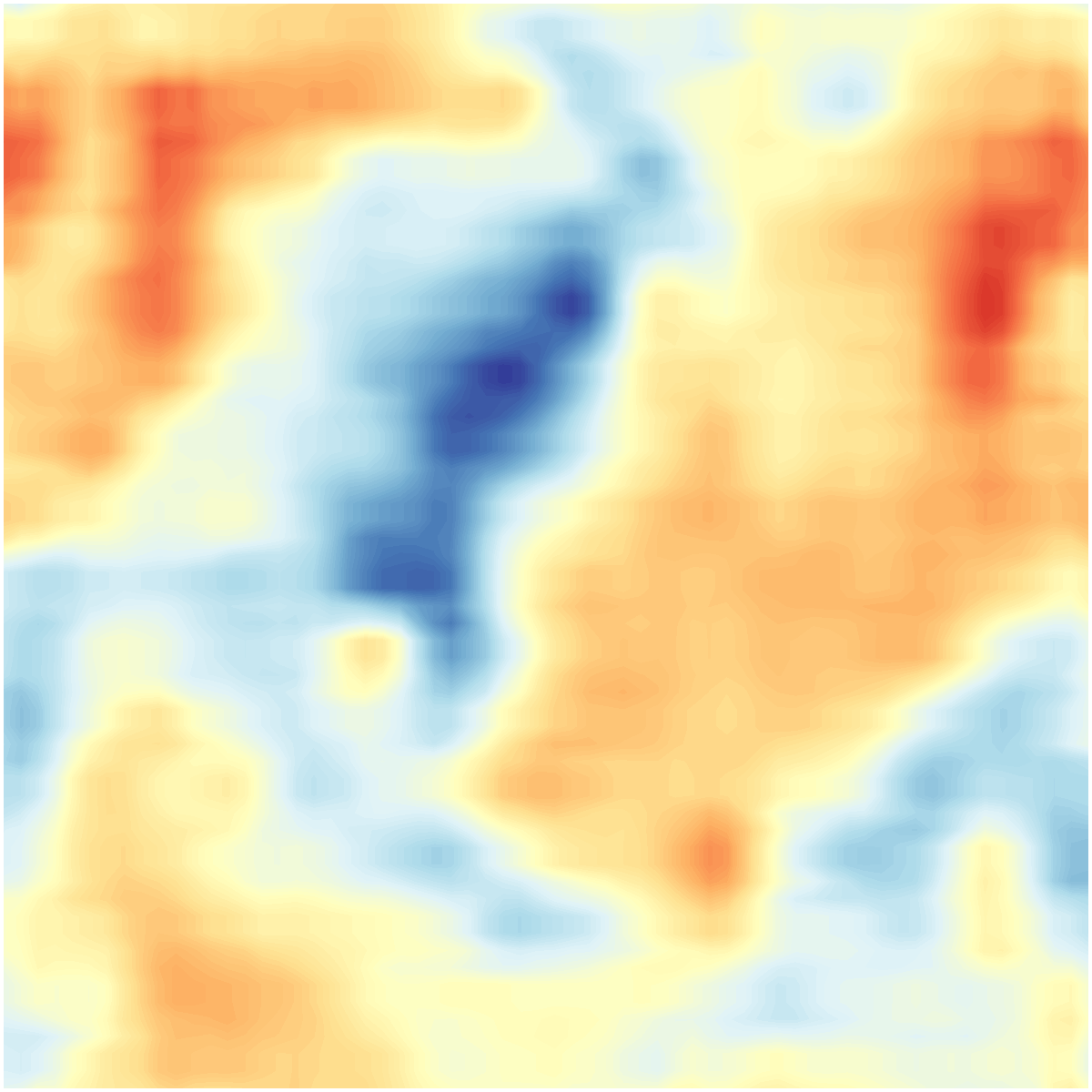
(b) DCS/MS.

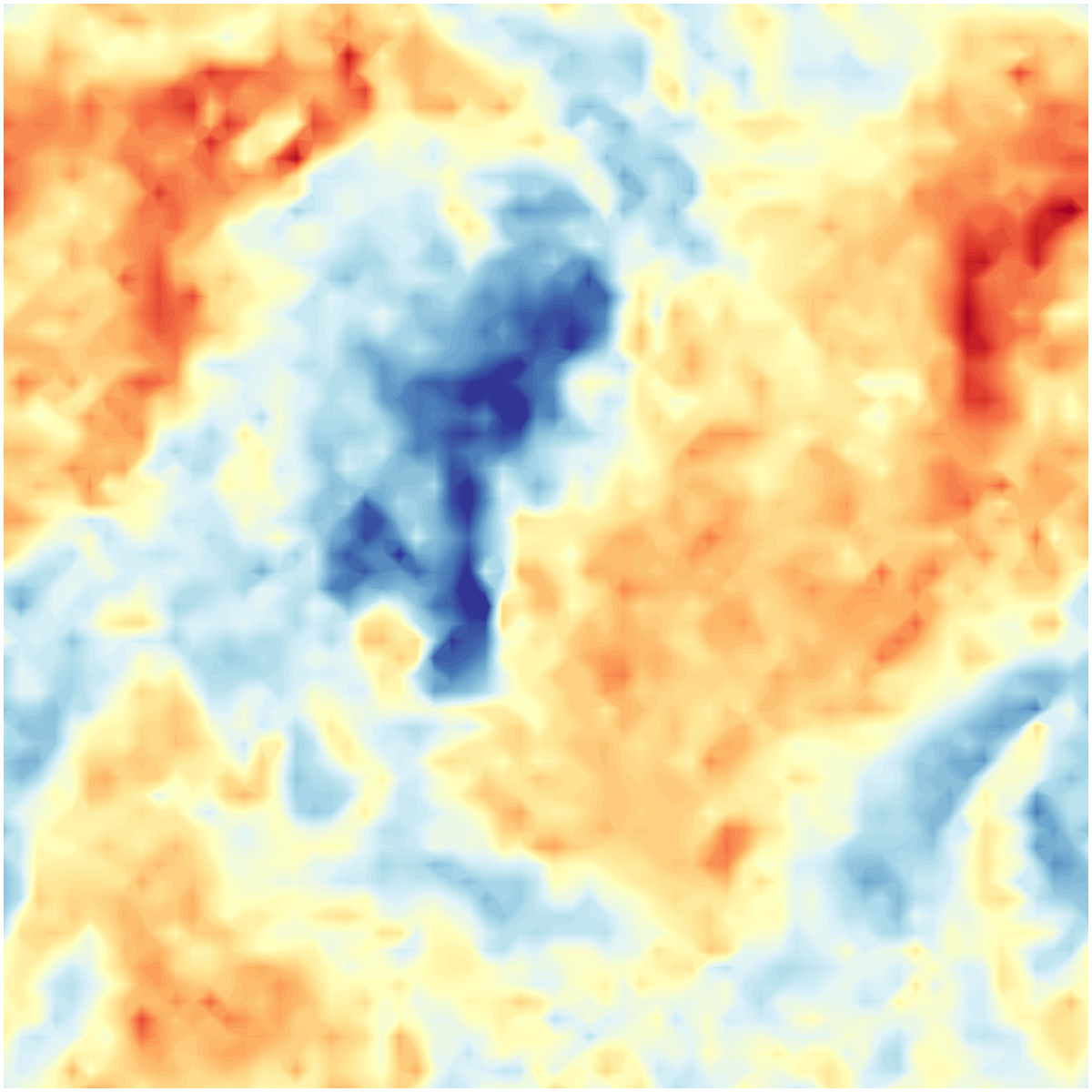
(c) CTN.

(d) CNDE-E.

(e) CNDE-R.

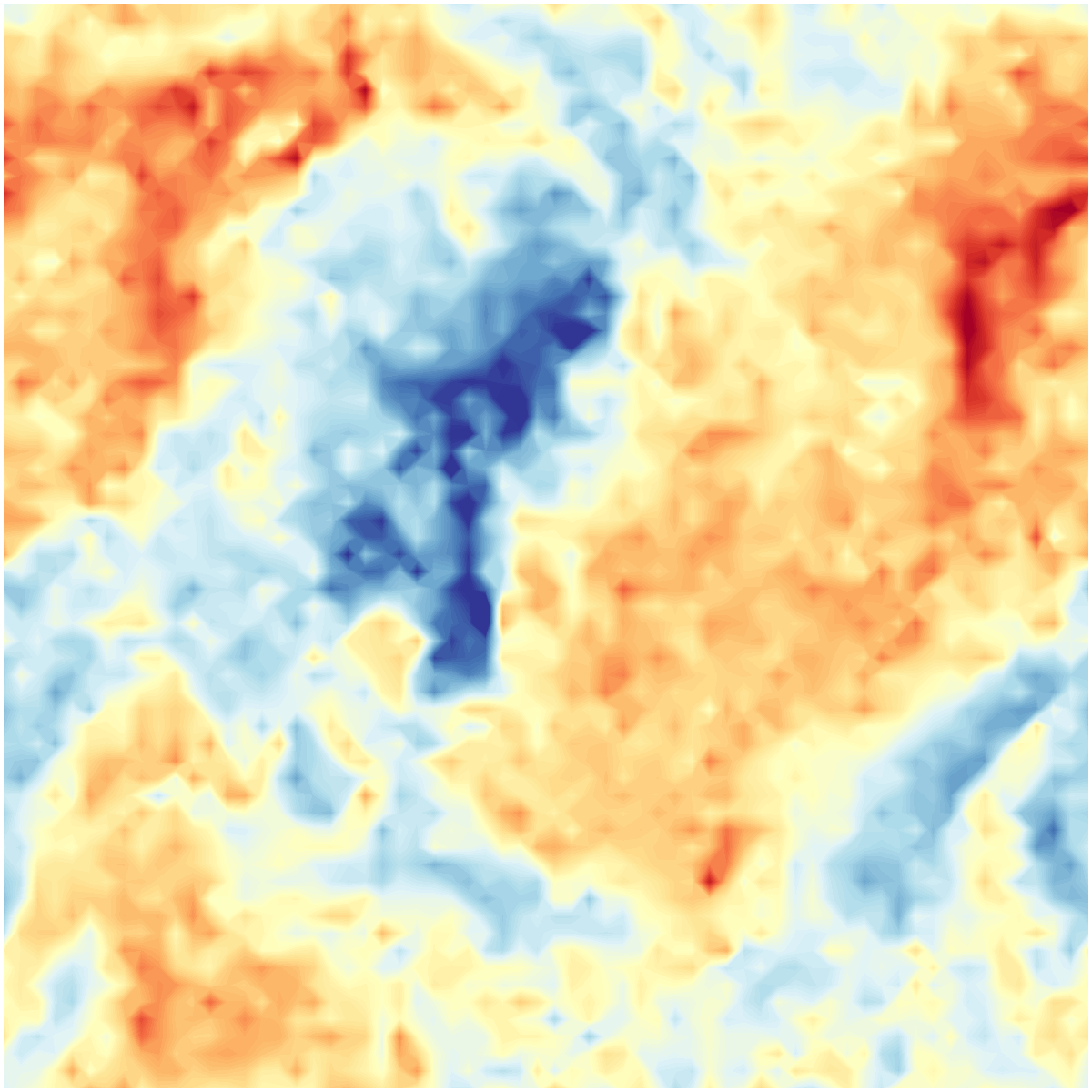
(f) Target DNS.

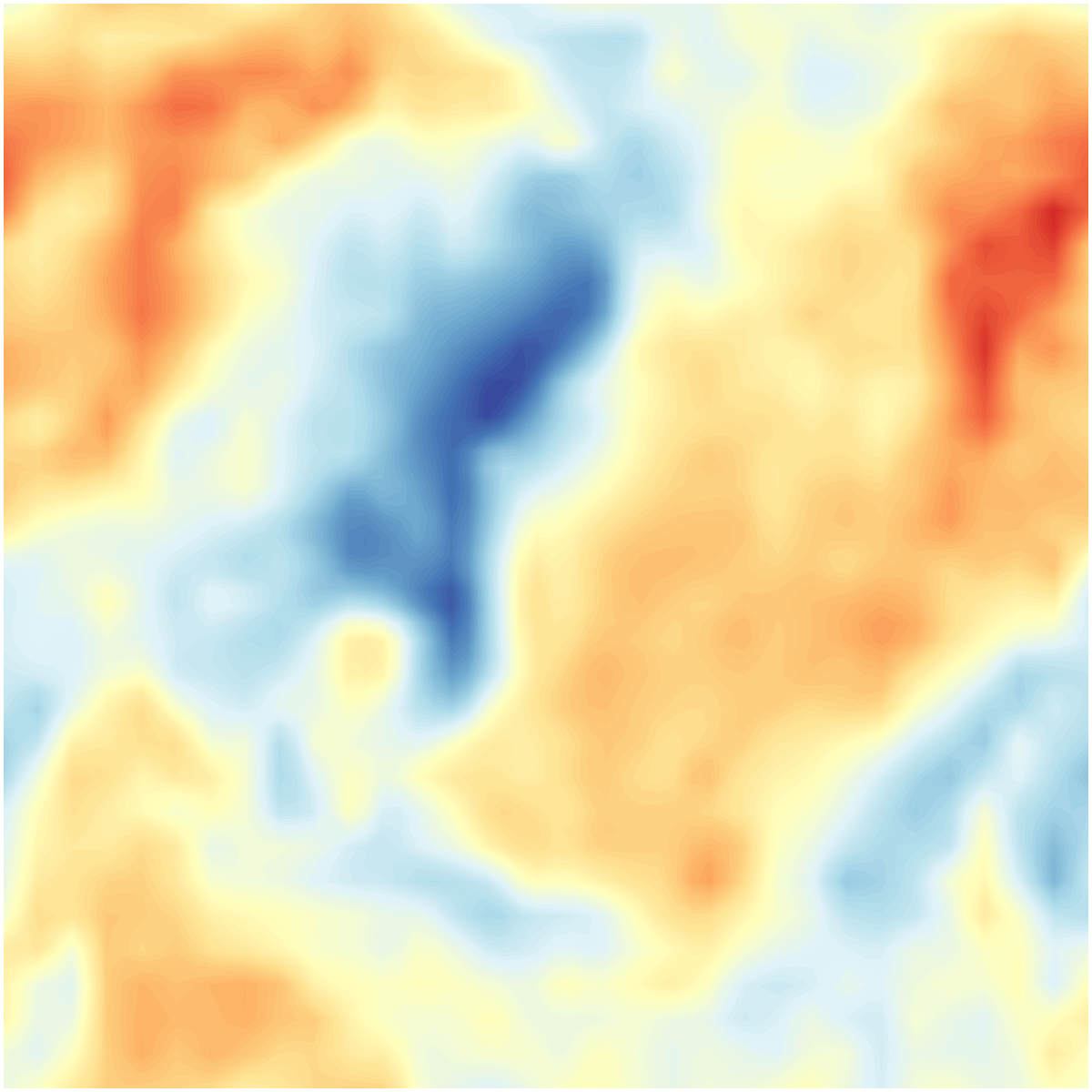
(g) LES Upsampling.

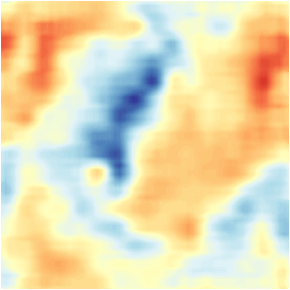
(h) DCS/MS.

(i) CTN.

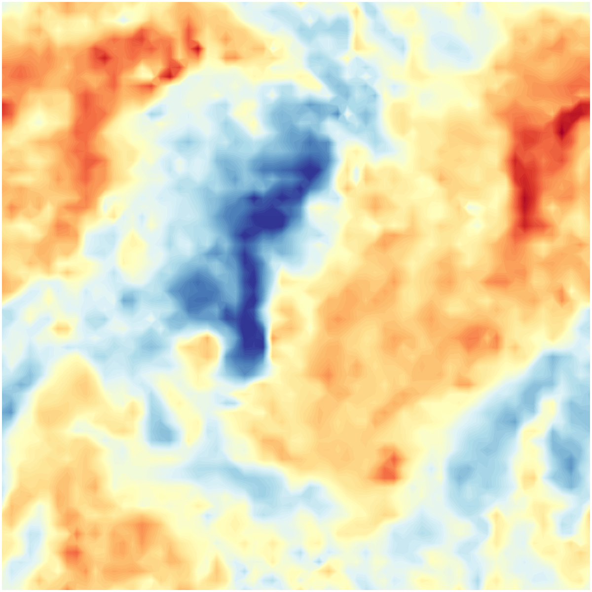
(j) CNDE-E.

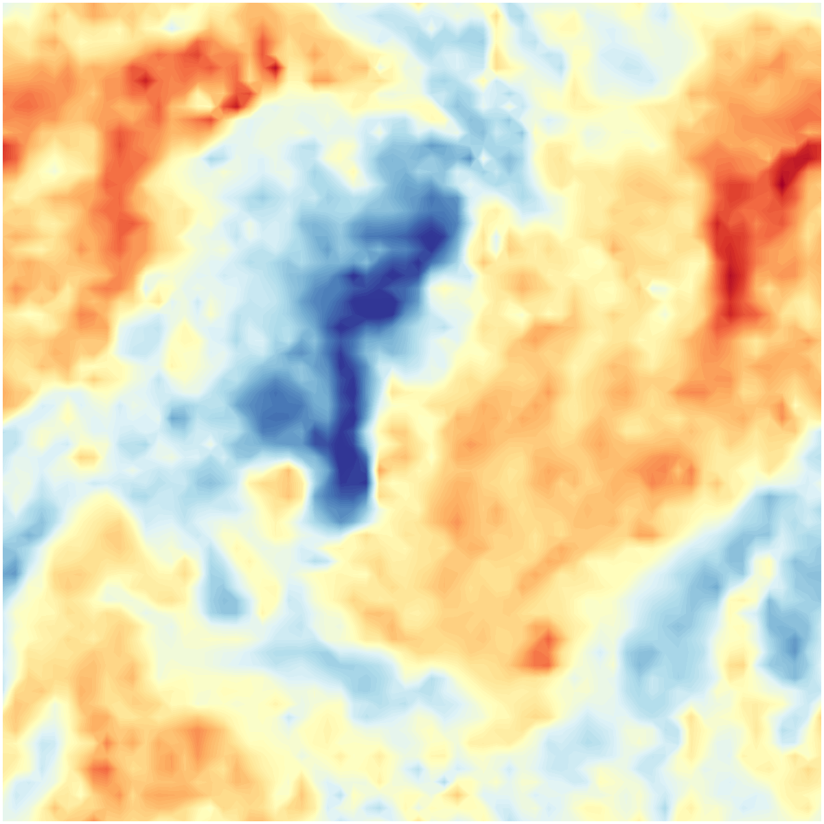
(k) CNDE-R.

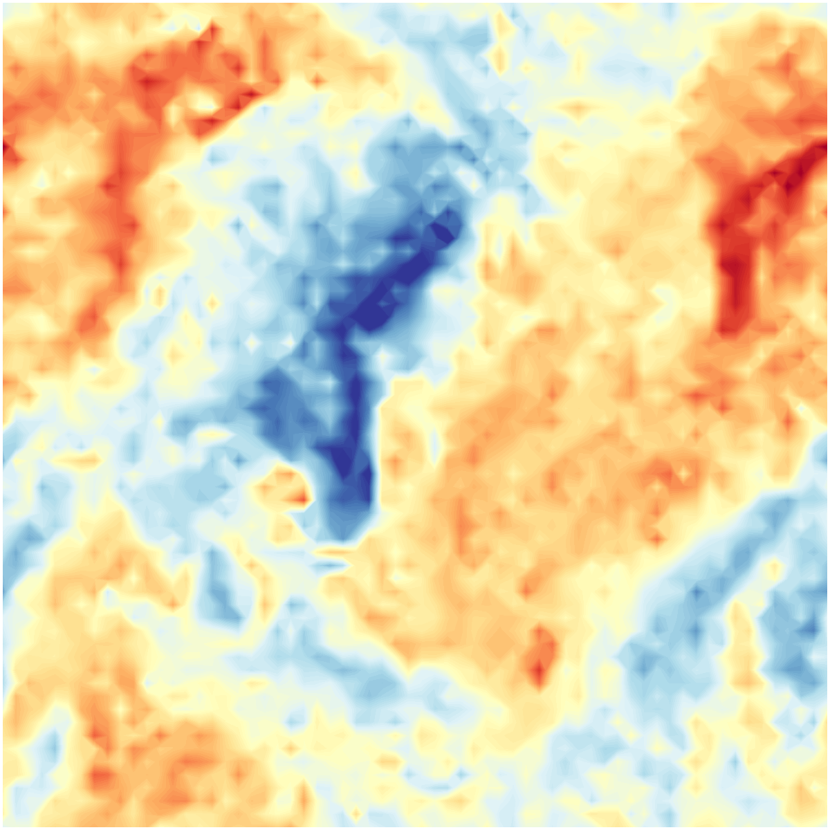
(l) Target DNS.

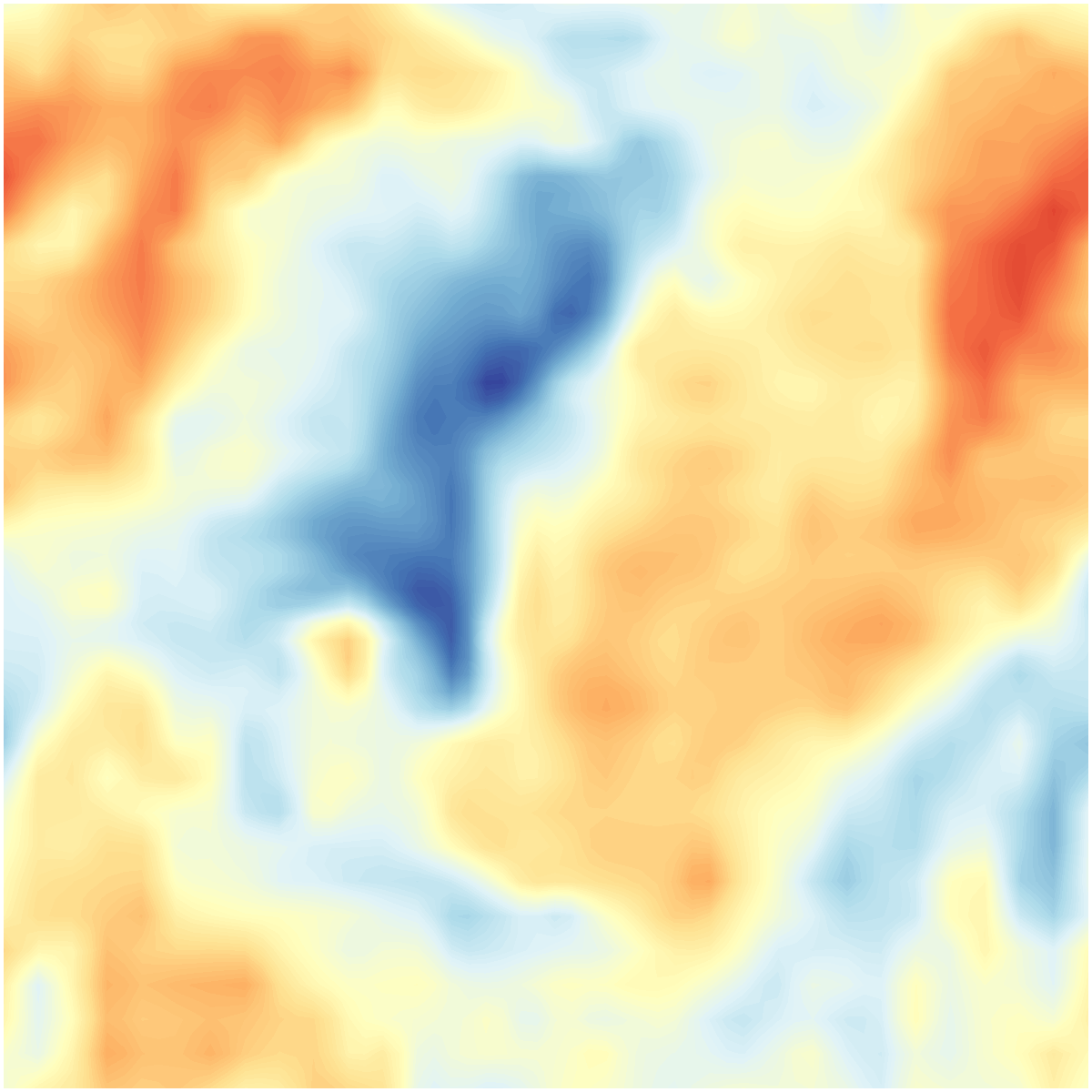
(m) LES Upsampling.

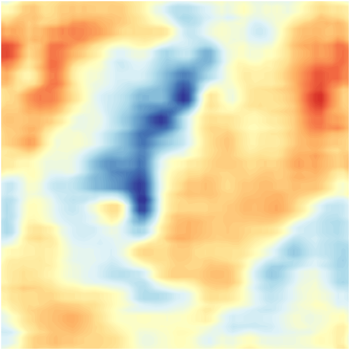
(n) DCS/MS.

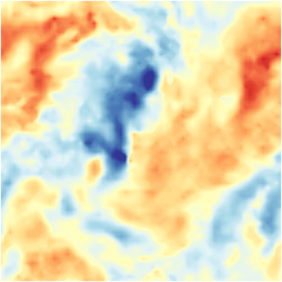
(o) CTN.

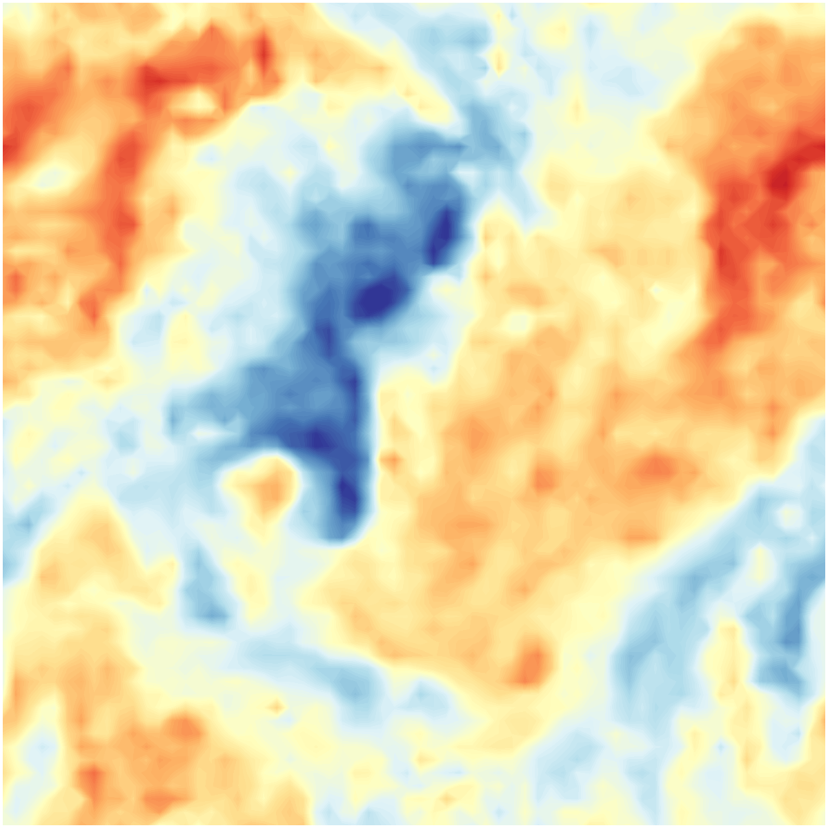
(p) CNDE-E.

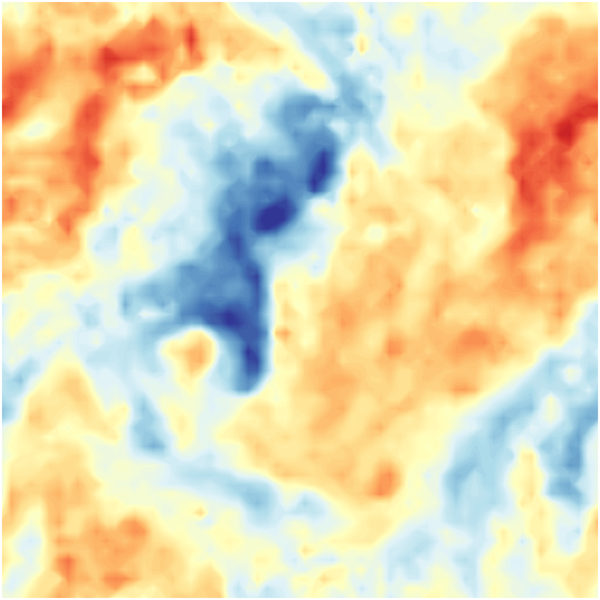
(q) CNDE-R.

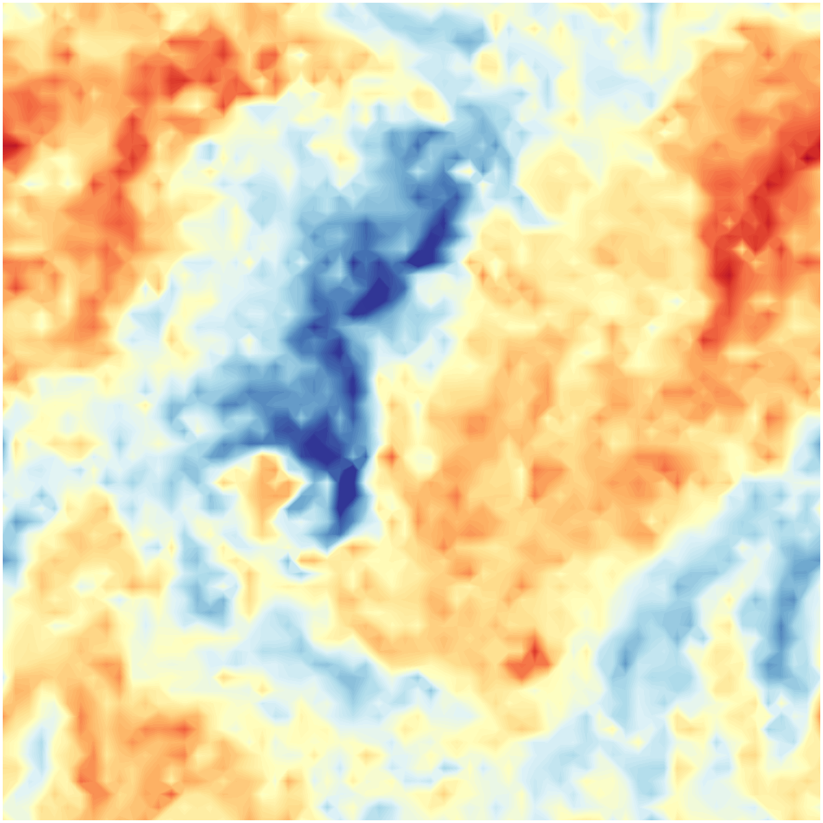
(r) Target DNS.

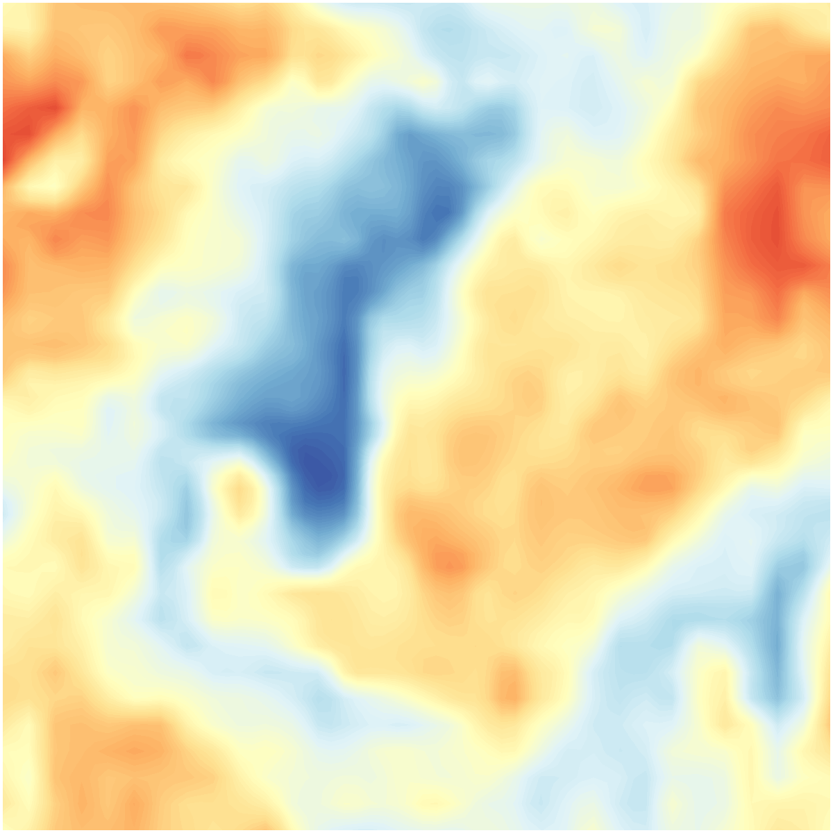
(s) LES Upsampling.

(t) DCS/MS.

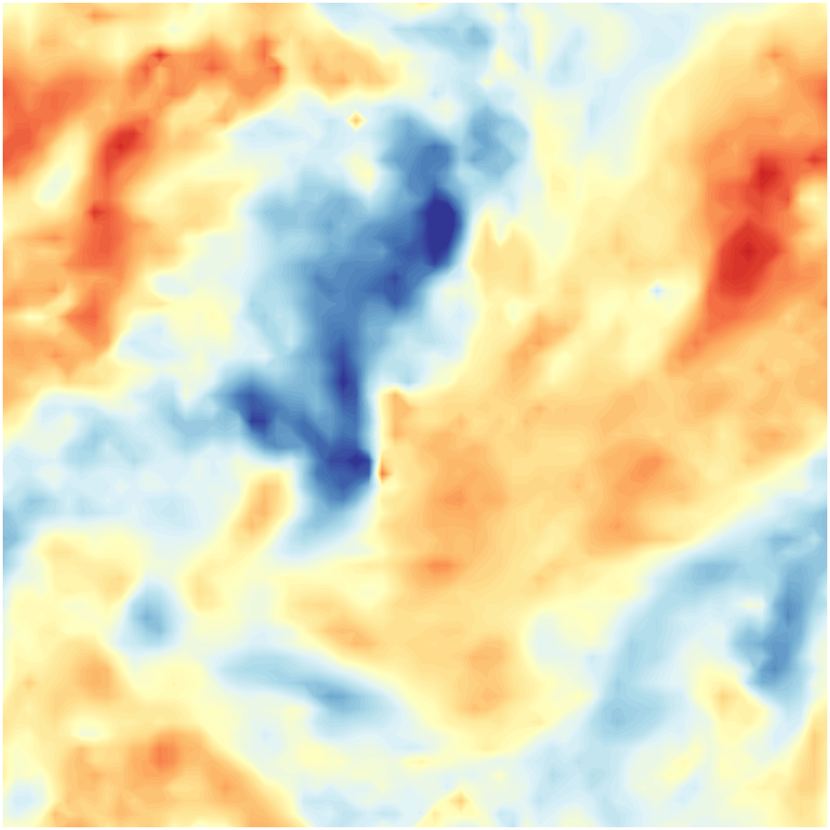
(u) CTN.

(v) CNDE-E.

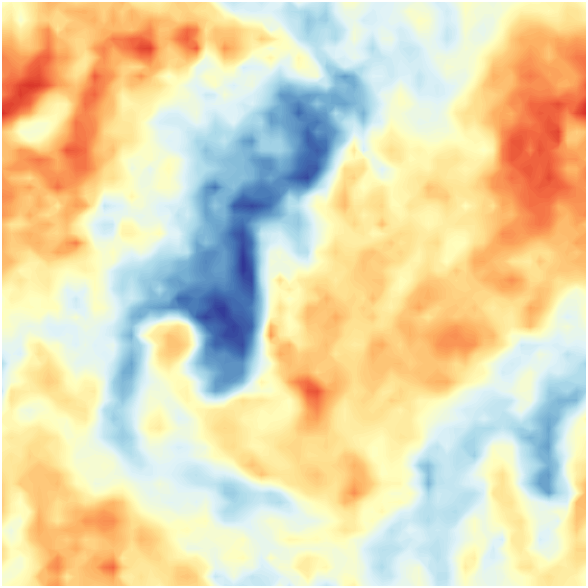
(w) CNDE-R.

(x) Target DNS.

Figure 8. Reconstructed $w$ channel by each method on a sample testing slice along the $z$ dimension in the FIT dataset. The reconstruction results are shown at 1st (7s), 5th (7.1s) 10th (7.2s) and 20th (7.4s) in (a)-(f), (g)-(l), (m)-(r) and (s)-(x), respectively.

(a) LES Upsampling.

(b) DCS/MS.

(c) CTN.

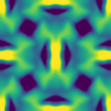
(d) CNDE-E.

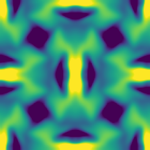
(e) CNDE-R.

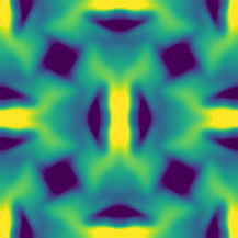
(f) Target DNS.

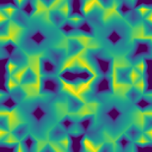
(g) LES Upsampling.

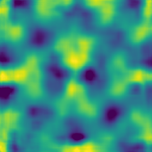
(h) DCS/MS.

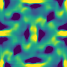
(i) CTN.

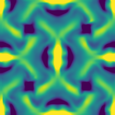
(j) CNDE-E.

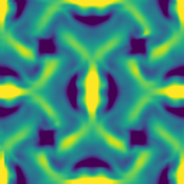
(k) CNDE-R.

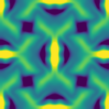
(l) Target DNS.

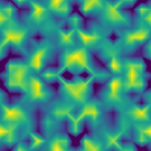
(m) LES Upsampling.

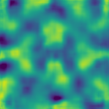
(n) DCS/MS.

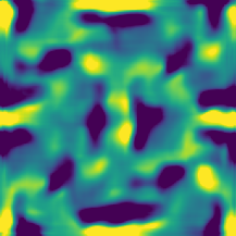
(o) CTN.

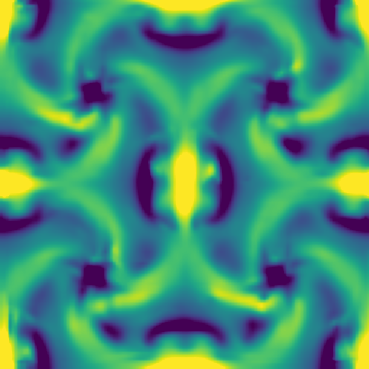
(p) CNDE-E.

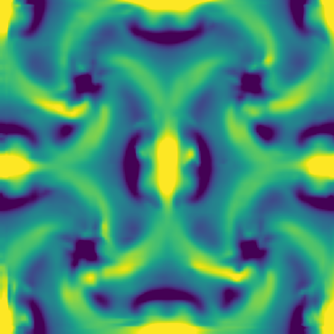
(q) CNDE-R.

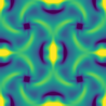
(r) Target DNS.

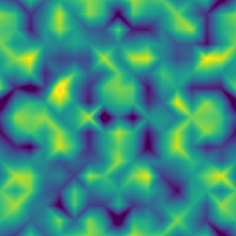
(s) LES Upsampling.

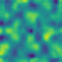
(t) DCS/MS.

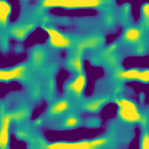
(u) CTN.

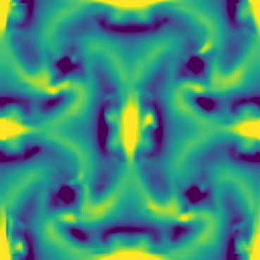
(v) CNDE-E.

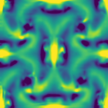
(w) CNDE-R.

(x) Target DNS.

Figure 9. Reconstructed $w$ channel by each method on a sample testing slice along the $z$ dimension in the TGV dataset. The reconstruction results are shown at 1st (80s), 5th (90s), 10th (100s), and 15th (110s) in (a)-(f), (g)-(l), (m)-(r) and (s)-(x), respectively.

4.2.2. Experimental Designs

The proposed methods and the baselines are tested on both the FIT and the TGV datasets. The models are trained by using the FIT data from a consecutive one-second period with a time interval $\delta=0.02s$ and a total of $50$ time steps, and then apply the trained model into the next $0.4$ second period (a total of $20$ time steps) for performance evaluation. For the TGV dataset, the models use a consecutive $40$-second period with a time interval $\delta=2s$ for training and the next $40$ seconds of data for testing.

The performance of DNS reconstruction is evaluated by using two different metrics, structural similarity index measure (SSIM) (Wang et al., 2004), and dissipation  (Wikipedia contributors, 2022b). SSIM is used to appraise the similarity between reconstructed data and target DNS on three aspects, luminance, contrast, and overall structure. The higher value of SSIM indicates better reconstruction performance. The dissipation operator is used to assess the performance of capturing the flow gradients. The dissipation of each of the three components of the velocity vector ($u$, $v$, and $w$) are evaluated. The dissipation operator is defined by:

(16) $$\chi(Q)\equiv\nabla Q\cdot\nabla Q=\left(\frac{\partial Q}{\partial x}\right)^{2}+\left(\frac{\partial Q}{\partial y}\right)^{2}+\left(\frac{\partial Q}{\partial z}\right)^{2}.$$

The dissipation is used to measure the difference of flow gradient between the true DNS and generated data. This is represented by $|\chi({Q}^{d})-\chi(\hat{{Q}}^{d})|$. The lower value of this difference indicates better performance. Compared with our previous work (Bao et al., 2022), the performance assessment is expanded by considering a new pixel-wise evaluation metric (dissipation) and a physical validation method based on the kinetic energy.

4.2.3. Environmental Settings and Implementation Details

The method is implemented via Tensorflow 2 with a GTX3080 GPU. The model is first trained in 500 epochs with ADAM optimizer (Kingma and Ba, 2014) from an initial learning rate of $0.001$. In the refinement step, the learning rate is lowered to $0.0005$, and the training rate is iterated by 10 epochs. All the hidden variables and gating variables are in $32$ dimensions. The values of $\alpha_{0}$, $\alpha_{1}$, and $\alpha_{2}$ are set as $1,\ 0.1,$ and $0.1$, respectively.

4.3. Reconstruction Performance

4.3.1. Quantitative Results.

Table 1 and Table 2 summarize the average performance over the first $10$ time steps in the testing phase on both the FIT dataset and the TGV dataset. Compared with the baselines, CNDE-based methods perform the best in both evaluations obtaining the highest SSIM value and lowest dissipation difference. Several observations are made: (1) When comparing the CNDE-based methods with SR baselines, DCS/MS, FNO, and FSR models, it is observed that these baseline methods cannot recover the overall flow well and get worse performance in terms of SSIM and dissipation difference. (2) Compared with the SRCNN, the CTN, which uses the LSTM model, shows a significant improvement in both evaluations. This confirms the effectiveness of a temporal model (e.g., LSTM) in capturing temporal dependency. (3) The comparison between CTN, RKTU, CNDEp-based methods, and CNDE-based methods, indicates significant improvements by incorporating each of the three components (RKTU, TEL, and refinement). In particular, the refinement method brings the most significant improvement in terms of SSIM and dissipation differences.

4.3.2. Temporal Analysis.

In the temporal analysis of the FIT dataset, the performance for reconstruction is measured for each step during a $0.4s$ period ($20$ time steps) in the testing phase. The performance change using the SSIM and the dissipation difference is shown in Figs. 4 and  5, respectively. These figures indicate that: (1) With larger time intervals between training data and prediction data, the performance becomes worse. In general, the CNDE-based methods are more stable over a long period, and show a much better performance than other methods. (2) The temporal model (e.g. LSTM) resutls in significant improvements in long-term predictions. (3) The CNDE-based methods outperform the CNDEp-based methods, which demonstrate the effectiveness of test-time refinement in reducing the prediction bias in long-term prediction. (4) The CNDEp-based methods yield a better performance after the 5th time steps compared with the temporal baseline CTN model. This indicates the advantage of the RKTU structure in the long-term prediction. (5) The CNDEp-E slightly outperforms the CNDEp-R in the long-term prediction. A similar observation is made by comparing two versions of CNDE-based methods.

In Figs. 6 and  7, the results for the TGV are presented. A better performance of the model developed here is indicated via the SSIM and dissipation differences. Several observations are made: (1) The CNDE-based methods using refinement perform much better than CNDEp-based methods and DCS/MS. Moreover, the performance of the CNDEp-based methods becomes worse than the baseline DCS/MS after the 5th time step. This is because of the variability of TGV data over larger time intervals ($\delta=2$s) and the testing data are very different from the initial data point. This causes the CNDEp-based methods to fail in capturing the correct flow dynamic without refinement. It also indicates the advantages of the refinement method for adjusting the state of flow data in the long-term prediction. (2) The CTN almost fails to capture the flow dynamics after the 5th time step, thus the CTN is not suitable for this dataset.

4.3.3. Visualization.

In Figs. 8, the reconstructed data are shown at multiple (1st, 5th, 10th, and 20th) time steps after the training period. For each time step, the slices of the $w$ component at a specified $z$ value are shown. In the 1st step, both the CNDE-based methods and the baseline CTN model yield ideal reconstruction results. This is because the test data are similar to the training data at the last time step. In contrast, the baseline DSC/MS (Fukami et al., 2019) leads to a poor performance starting from early time. Beginning at the 5th time step, the CNDE-based methods perform better than the baselines. A more significant difference is observed at the 20th time step. All the baselines almost fail to capture the correct flow transport pattern. The CNDE-based methods yield a much better performance in the late stage. Similar observations are made on the TGV dataset as shown in Fig. 9.

4.3.4. Validation via Physical Metrics.

The model performance is also assessed via of long-term prediction of the turbulent kinetic energy. Figure 10 show the energies corresponding to the target DNS, and the reconstructed flow data by the baselines and the CNDE-based methods for both the FIT and the TGV flows. The results in Fig. 10 (a) for the FIT dataset indicate: (1) The CNDE-based methods in general perform better than the baseline method DCS/MS and CTN. Even without using the refinement process, the CNDEp-based methods outperform the DCS/MS and CTN models. CNDE-based methods can follow the underlying physical rule well in the long-term prediction. (2) The performance of CNDEp-based methods becomes very poor after the 8th time step. This is because the accumulated error gets amplified in every time step. The results in Fig. 10 (b) yield similar conclusions.

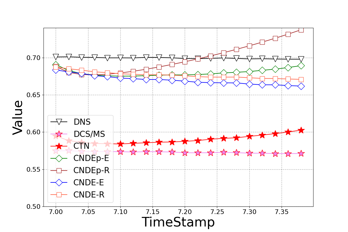
(a) FIT data.

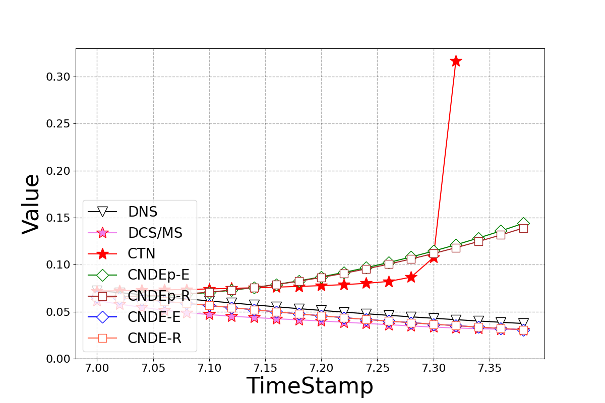
(b) TGV data.

Figure 10. Change of kinetic energy produced by the reference DNS and different models in both the FIT and the TGV datasets, respectively.

5. Summary & Concluding Remarks

A novel super-resolution (SR) methodology, termed “continuous networks using differential equations” (CNDE) is developed to reconstruct high-resolution flow data in spatial and temporal fields. The model is used in the setting of unsteady, incompressible, Newtonian turbulent flow under spatially homogeneous conditions. The SR method is to generate the high resolution direct numerical simulation (DNS) field from low resolution, large eddy simulation (LES) data. A Runge-Kutta transition unit (RKTU) is developed to leverage the physical knowledge embodied in the Navier-Stokes equation to capture the spatial resolution, and the temporal dynamics of the flow. A temporally-enhancing layer (TEL) is constructed to capture long-term temporal dynamics. A degradation-based refinement method is developed to adjust the reconstructed data over time by enforcing the consistency with physical constraints. The performance of the model is assessed in the setting of two flow configurations via flow visualization and statistical analysis. The results demonstrate the superiority of the CNDE for spatio-temporal reconstruction of the flow. The model’s constituents, the RKTU and the refinement methods can be used as building blocks to enhance existing deep learning models.

Despite its demonstrated capabilities, there are two limitations associated with the CNDE model in its current form. (1) The CNN layers are used to estimate spatial derivatives, which can introduce bias due to the approximation and due to data overfitting. (2) The method is, thus far, tailored and appraised for specific flows. Therefore, its generality cannot be warranted for other applications; especially in the absence of sufficient DNS data. Future work is recommended to find alternative ways to evaluate the spatial derivatives more accurately and to improve the model’s transferability.

- (1)
- Ahn et al. (2018) Namhyuk Ahn, Byungkon Kang, and Kyung-Ah Sohn. 2018. Fast, accurate, and lightweight super-resolution with cascading residual network. In Proceedings of the European conference on computer vision (ECCV). 252–268.
- Albawi et al. (2017) Saad Albawi, Tareq Abed Mohammed, and Saad Al-Zawi. 2017. Understanding of a convolutional neural network. In 2017 international conference on engineering and technology (ICET). IEEE, 1–6.
- Bao et al. (2022) Tianshu Bao, Shengyu Chen, Taylor T Johnson, Peyman Givi, Shervin Sammak, and Xiaowei Jia. 2022. Physics Guided Neural Networks for Spatio-temporal Super-resolution of Turbulent Flows. In The 38th Conference on Uncertainty in Artificial Intelligence.
- Boussif et al. (2022) Oussama Boussif, Yoshua Bengio, Loubna Benabbou, and Dan Assouline. 2022. MAgnet: Mesh agnostic neural PDE solver. Advances in Neural Information Processing Systems 35 (2022), 31972–31985.
- Brachet et al. (1984) Marc E Brachet, D Meiron, S Orszag, B Nickel, R Morf, and Uriel Frisch. 1984. The Taylor-Green vortex and fully developed turbulence. Journal of Statistical Physics 34, 5 (1984), 1049–1063.
- Butcher (2007) John Butcher. 2007. Runge-kutta methods. Scholarpedia 2, 9 (2007), 3147.
- Chen et al. (2023) Shengyu Chen, Nasrin Kalanat, Yiqun Xie, Sheng Li, Jacob A Zwart, Jeffrey M Sadler, Alison P Appling, Samantha K Oliver, Jordan S Read, and Xiaowei Jia. 2023. Physics-guided machine learning from simulated data with different physical parameters. Knowledge and Information Systems 65, 8 (2023), 3223–3250.
- Chen et al. (2021) Shengyu Chen, Shervin Sammak, Peyman Givi, Joseph P Yurko, and Xiaowei Jia. 2021. Reconstructing high-resolution turbulent flows using physics-guided neural networks. In 2021 IEEE International Conference on Big Data (Big Data). IEEE, 1369–1379.
- Chen et al. (2022) Shengyu Chen, Jacob A Zwart, and Xiaowei Jia. 2022. Physics-guided graph meta learning for predicting water temperature and streamflow in stream networks. In Proceedings of the 28th ACM SIGKDD Conference on Knowledge Discovery and Data Mining. 2752–2761.
- Chen et al. (2018) Yu Chen, Ying Tai, Xiaoming Liu, Chunhua Shen, and Jian Yang. 2018. Fsrnet: End-to-end learning face super-resolution with facial priors. In Proceedings of the IEEE conference on computer vision and pattern recognition. 2492–2501.
- Cheng et al. (2021) Wenlong Cheng, Mingbo Zhao, Zhiling Ye, and Shuhang Gu. 2021. Mfagan: A compression framework for memory-efficient on-device super-resolution gan. arXiv preprint arXiv:2107.12679 (2021).
- Dai et al. (2019) Tao Dai, Jianrui Cai, Yongbing Zhang, Shu-Tao Xia, and Lei Zhang. 2019. Second-Order Attention Network for Single Image Super-Resolution. In 2019 IEEE/CVF Conference on Computer Vision and Pattern Recognition (CVPR). 11057–11066. https://doi.org/10.1109/CVPR.2019.01132
- Daw et al. (2022) Arka Daw, Anuj Karpatne, William D Watkins, Jordan S Read, and Vipin Kumar. 2022. Physics-guided neural networks (pgnn): An application in lake temperature modeling. In Knowledge Guided Machine Learning. Chapman and Hall/CRC, 353–372.
- Deng et al. (2019) Zhiwen Deng, Chuangxin He, Yingzheng Liu, and Kyung Chun Kim. 2019. Super-resolution reconstruction of turbulent velocity fields using a generative adversarial network-based artificial intelligence framework. Physics of Fluids 31, 12 (2019), 125111.
- Dong et al. (2014) Chao Dong, Chen Change Loy, Kaiming He, and Xiaoou Tang. 2014. Learning a deep convolutional network for image super-resolution. In Computer Vision–ECCV 2014: 13th European Conference, Zurich, Switzerland, September 6-12, 2014, Proceedings, Part IV 13. Springer, 184–199.
- Equer et al. (2023) Léonard Equer, T Konstantin Rusch, and Siddhartha Mishra. 2023. Multi-scale message passing neural pde solvers. arXiv preprint arXiv:2302.03580 (2023).
- Fang et al. (2022b) Chaowei Fang, Dingwen Zhang, Liang Wang, Yulun Zhang, Lechao Cheng, and Junwei Han. 2022b. Cross-modality high-frequency transformer for mr image super-resolution. In Proceedings of the 30th ACM International Conference on Multimedia. 1584–1592.
- Fang et al. (2022a) Jinsheng Fang, Hanjiang Lin, Xinyu Chen, and Kun Zeng. 2022a. A hybrid network of cnn and transformer for lightweight image super-resolution. In Proceedings of the IEEE/CVF conference on computer vision and pattern recognition. 1103–1112.
- Fukami et al. (2019) Kai Fukami, Koji Fukagata, and Kunihiko Taira. 2019. Super-resolution reconstruction of turbulent flows with machine learning. Journal of Fluid Mechanics 870 (2019), 106–120.
- Fukami et al. (2021) Kai Fukami, Koji Fukagata, and Kunihiko Taira. 2021. Machine-learning-based spatio-temporal super resolution reconstruction of turbulent flows. Journal of Fluid Mechanics 909 (2021), A9.
- Givi (1994) P. Givi. 1994. Spectral and Random Vortex Methods in Turbulent Reacting Flows. In Turbulent Reacting Flows, P. A. Libby and F. A. Williams (Eds.). Academic Press, London, England, Chapter 8, 475–572.
- Hanson et al. (2020) Paul C Hanson et al. 2020. Predicting lake surface water phosphorus dynamics using process-guided machine learning. Ecological Modelling 430 (2020), 109136.
- He et al. (2023) Erhu He, Yiqun Xie, Licheng Liu, Weiye Chen, Zhenong Jin, and Xiaowei Jia. 2023. Physics Guided Neural Networks for Time-Aware Fairness: An Application in Crop Yield Prediction. In Proceedings of the AAAI Conference on Artificial Intelligence, Vol. 37. 14223–14231.
- Hochreiter and Schmidhuber (1997) Sepp Hochreiter and Jürgen Schmidhuber. 1997. Long short-term memory. Neural computation 9, 8 (1997), 1735–1780.
- Jia et al. (2023) Xiaowei Jia, Shengyu Chen, Can Zheng, Yiqun Xie, Zhe Jiang, and Nasrin Kalanat. 2023. Physics-guided Graph Diffusion Network for Combining Heterogeneous Simulated Data: An Application in Predicting Stream Water Temperature. In Proceedings of the 2023 SIAM International Conference on Data Mining (SDM). SIAM, 361–369.
- Jia et al. (2019) Xiaowei Jia, Jared Willard, Anuj Karpatne, Jordan Read, Jacob Zwart, Michael Steinbach, and Vipin Kumar. 2019. Physics guided RNNs for modeling dynamical systems: A case study in simulating lake temperature profiles. In Proceedings of the 2019 SIAM international conference on data mining. SIAM, 558–566.
- Jing et al. (2000) Cai Jing, Yang Jinsheng, and Ding Runtao. 2000. Fuzzy weighted average filter. In WCC 2000-ICSP 2000. 2000 5th International Conference on Signal Processing Proceedings. 16th World Computer Congress 2000, Vol. 1. IEEE, 525–528.
- Karras et al. (2017) Tero Karras, Timo Aila, Samuli Laine, and Jaakko Lehtinen. 2017. Progressive growing of gans for improved quality, stability, and variation. arXiv preprint arXiv:1710.10196 (2017).
- Khandelwal et al. (2020) Ankush Khandelwal, Shaoming Xu, Xiang Li, Xiaowei Jia, Michael Stienbach, Christopher Duffy, John Nieber, and Vipin Kumar. 2020. Physics guided machine learning methods for hydrology. arXiv preprint arXiv:2012.02854 (2020).
- Kingma and Ba (2014) Diederik P Kingma and Jimmy Ba. 2014. Adam: A method for stochastic optimization. arXiv preprint arXiv:1412.6980 (2014).
- Lea et al. (2016) Colin Lea, Rene Vidal, Austin Reiter, and Gregory D Hager. 2016. Temporal convolutional networks: A unified approach to action segmentation. In European conference on computer vision. Springer, 47–54.
- Ledig et al. (2017) Christian Ledig, Lucas Theis, Ferenc Huszár, Jose Caballero, Andrew Cunningham, Alejandro Acosta, Andrew Aitken, Alykhan Tejani, Johannes Totz, Zehan Wang, et al. 2017. Photo-realistic single image super-resolution using a generative adversarial network. In Proceedings of the IEEE conference on computer vision and pattern recognition. 4681–4690.
- Li et al. (2020) Zongyi Li, Nikola Kovachki, Kamyar Azizzadenesheli, Burigede Liu, Kaushik Bhattacharya, Andrew Stuart, and Anima Anandkumar. 2020. Fourier neural operator for parametric partial differential equations. arXiv preprint arXiv:2010.08895 (2020).
- Liang et al. (2022) Zhengyu Liang, Yingqian Wang, Longguang Wang, Jungang Yang, and Shilin Zhou. 2022. Light field image super-resolution with transformers. IEEE Signal Processing Letters 29 (2022), 563–567.
- Liu et al. (2020) Bo Liu, Jiupeng Tang, Haibo Huang, and Xi-Yun Lu. 2020. Deep learning methods for super-resolution reconstruction of turbulent flows. Physics of Fluids 32, 2 (2020), 025105.
- Liu et al. (2022) Licheng Liu, Shaoming Xu, Jinyun Tang, Kaiyu Guan, Timothy J Griffis, Matthew D Erickson, Alexander L Frie, Xiaowei Jia, Taegon Kim, Lee T Miller, et al. 2022. KGML-ag: a modeling framework of knowledge-guided machine learning to simulate agroecosystems: a case study of estimating N 2 O emission using data from mesocosm experiments. Geoscientific Model Development 15, 7 (2022), 2839–2858.
- Lu et al. (2022) Zhisheng Lu, Juncheng Li, Hong Liu, Chaoyan Huang, Linlin Zhang, and Tieyong Zeng. 2022. Transformer for single image super-resolution. In Proceedings of the IEEE/CVF conference on computer vision and pattern recognition. 457–466.
- Minping et al. (2012) Wan Minping, Shiyi Chen, Gregory Eyink, Charles Meneveau, Perry Johnson, Eric Perlman, Randal Burns, Yi Li, Alex Szalay, and Stephen Hamilton. 2012. Forced Isotropic Turbulence Data Set (Extended). (2012).
- Muralidhar et al. (2020) Nikhil Muralidhar, Jie Bu, Ze Cao, Long He, Naren Ramakrishnan, Danesh Tafti, and Anuj Karpatne. 2020. PhyNet: Physics Guided Neural Networks for Particle Drag Force Prediction in Assembly. In Proceedings of the 2020 SIAM International Conference on Data Mining. SIAM, 559–567.
- Nouri et al. (2017) Arash G Nouri, Mehdi B Nik, Pope Givi, Daniel Livescu, and Stephen B Pope. 2017. Self-contained filtered density function. Physical Review Fluids 2, 9 (2017), 094603.
- Park et al. (2003) Sung Cheol Park, Min Kyu Park, and Moon Gi Kang. 2003. Super-resolution image reconstruction: a technical overview. IEEE signal processing magazine 20, 3 (2003), 21–36.
- Parmar et al. (2018) Niki Parmar, Ashish Vaswani, Jakob Uszkoreit, Lukasz Kaiser, Noam Shazeer, Alexander Ku, and Dustin Tran. 2018. Image transformer. In International conference on machine learning. PMLR, 4055–4064.
- Read et al. (2019) Jordan S Read, Xiaowei Jia, Jared Willard, Alison P Appling, Jacob A Zwart, Samantha K Oliver, Anuj Karpatne, Gretchen JA Hansen, Paul C Hanson, William Watkins, et al. 2019. Process-guided deep learning predictions of lake water temperature. Water Resources Research 55, 11 (2019), 9173–9190.
- Sagaut (2005) Pierre Sagaut. 2005. Large eddy simulation for incompressible flows: an introduction. Springer Science & Business Media.
- Tai et al. (2017) Ying Tai, Jian Yang, and Xiaoming Liu. 2017. Image super-resolution via deep recursive residual network. In Proceedings of the IEEE conference on computer vision and pattern recognition. 3147–3155.
- Upadhyay and Awate (2019) Uddeshya Upadhyay and Suyash P Awate. 2019. Robust super-resolution GAN, with manifold-based and perception loss. In 2019 IEEE 16th International Symposium on Biomedical Imaging (ISBI 2019). IEEE, 1372–1376.
- Van Duong et al. (2021) Vinh Van Duong, Thuc Nguyen Huu, Jonghoon Yim, and Byeungwoo Jeon. 2021. A fast and efficient super-resolution network using hierarchical dense residual learning. In 2021 IEEE International Conference on Image Processing (ICIP). IEEE, 1809–1813.
- Vaswani et al. (2017) Ashish Vaswani, Noam Shazeer, Niki Parmar, Jakob Uszkoreit, Llion Jones, Aidan N Gomez, Łukasz Kaiser, and Illia Polosukhin. 2017. Attention is all you need. Advances in neural information processing systems 30 (2017).
- Wang et al. (2022) Shunzhou Wang, Tianfei Zhou, Yao Lu, and Huijun Di. 2022. Detail-preserving transformer for light field image super-resolution. In Proceedings of the AAAI Conference on Artificial Intelligence, Vol. 36. 2522–2530.
- Wang et al. (2018a) Xintao Wang, Ke Yu, Chao Dong, and Chen Change Loy. 2018a. Recovering realistic texture in image super-resolution by deep spatial feature transform. In Proceedings of the IEEE conference on computer vision and pattern recognition. 606–615.
- Wang et al. (2018b) Xintao Wang, Ke Yu, Shixiang Wu, Jinjin Gu, Yihao Liu, Chao Dong, Yu Qiao, and Chen Change Loy. 2018b. Esrgan: Enhanced super-resolution generative adversarial networks. In ECCV Workshops.
- Wang et al. (2004) Zhou Wang, Alan C Bovik, Hamid R Sheikh, and Eero P Simoncelli. 2004. Image quality assessment: from error visibility to structural similarity. IEEE transactions on image processing 13, 4 (2004), 600–612.
- Wenlong et al. (2021) Zhang Wenlong, Liu Yihao, Chao Dong, and Yu Qiao. 2021. RankSRGAN: Generative Adversarial Networks with Ranker for Image Super-Resolution. IEEE Transactions on Pattern Analysis and Machine Intelligence 44, 10 (2021), 1–1.
- Wikipedia contributors (2022a) Wikipedia contributors. 2022a. Finite difference method — Wikipedia, The Free Encyclopedia. https://en.wikipedia.org/w/index.php?title=Finite_difference_method&oldid=1126400243 [Online; accessed 25-January-2023].
- Wikipedia contributors (2022b) Wikipedia contributors. 2022b. Laplace operator — Wikipedia, The Free Encyclopedia. https://en.wikipedia.org/w/index.php?title=Laplace_operator&oldid=1127277109 [Online; accessed 23-January-2023].
- Willard et al. (2022) Jared Willard, Xiaowei Jia, Shaoming Xu, Michael Steinbach, and Vipin Kumar. 2022. Integrating scientific knowledge with machine learning for engineering and environmental systems. Comput. Surveys 55, 4 (2022), 1–37.
- Xie et al. (2018) You Xie, Erik Franz, Mengyu Chu, and Nils Thuerey. 2018. tempogan: A temporally coherent, volumetric gan for super-resolution fluid flow. ACM Transactions on Graphics (TOG) 37, 4 (2018), 1–15.
- Xu et al. (2023) Qin Xu, Zijian Zhuang, Yongcai Pan, and Binghai Wen. 2023. Super-resolution reconstruction of turbulent flows with a transformer-based deep learning framework. Physics of Fluids 35, 5 (2023).
- Yang et al. (2020) Fuzhi Yang, Huan Yang, Jianlong Fu, Hongtao Lu, and Baining Guo. 2020. Learning texture transformer network for image super-resolution. In Proceedings of the IEEE/CVF conference on computer vision and pattern recognition. 5791–5800.
- Yang et al. (2023) Zhen Yang, Hua Yang, and Zhouping Yin. 2023. Super-resolution reconstruction for the three-dimensional turbulence flows with a back-projection network. Physics of Fluids 35, 5 (2023).
- Zhang et al. (2018a) Yulun Zhang, Kunpeng Li, Kai Li, Lichen Wang, Bineng Zhong, and Yun Fu. 2018a. Image super-resolution using very deep residual channel attention networks. In Proceedings of the European conference on computer vision (ECCV). 286–301.
- Zhang et al. (2018b) Yulun Zhang, Yapeng Tian, Yu Kong, Bineng Zhong, and Yun Fu. 2018b. Residual Dense Network for Image Super-Resolution. arXiv preprint arXiv:1802.08797 (2018).
- Zou et al. (2022) Wenbin Zou, Tian Ye, Weixin Zheng, Yunchen Zhang, Liang Chen, and Yi Wu. 2022. Self-calibrated efficient transformer for lightweight super-resolution. In Proceedings of the IEEE/CVF Conference on Computer Vision and Pattern Recognition. 930–939.