Abstract
We consider two accelerating Unruh-DeWitt detectors coupled linearly or quadratically with a scalar field. We show that entanglement can be created by acceleration, and is divergent only when the two detectors coincide. For linear coupling, entanglment decreases monotonically with the increase of acceleration. For quadratic coupling, entanglement behaves non-monotonically.
1 Introduction
Quantum field theory in curved spacetime, in which the curvedness of the spacetime is considered but the gravity is not quantized Wald-1995 Unruh-1976 Hawking-1975 DeWitt-1979 ; Unruh-1984 Pozas-Kerstjens-2016 Φ ^ 2 superscript ^ Φ 2 \hat{\Phi}^{2} Takagi-1986 Sachs-2017
The Reeh-Schlieder theorem Reeh-1961 Maldacena-2003 Salton-2015
In this paper we focus on the entanglement harvesting of two uniformly accelerating detectors, both of which coupled quadratically with a scalar field. Other than working in the inertial frame, as in most of the previous studies, we tackle the problem from the Rindler observers’ perspective, which is more natural for our purpose, and the divergences appear only when these two detectors conincide in spacetime. Furthermore, for Φ 2 superscript Φ 2 \Phi^{2} Liu-2021 Yu-2009
This paper is organized as the following. In section 2 we will give a brief introduction to the Rindler modes, which are crucial in our calculation, and we will derive the reduced density matrix of our model which determines the entanglement properties. In section 3 and 4 we will study detectors that are linearly and quadratically coupled with the scalar field respectively. It can be seen that in these two different circumstances, the entanglement exhibits different features. In section 5, we will summarize our results and give an outlook.
2 Set up
Before we introduce the model, it is worthwhile to briefly review quantum field theory in the Rindler wedge since we will be working in the Rindler perspective.
The right Rindler coordinate ( τ , ξ , x , y ) 𝜏 𝜉 𝑥 𝑦 (\tau,\xi,x,y) ( t , x , y , z ) 𝑡 𝑥 𝑦 𝑧 (t,x,y,z)
t = a − 1 e a ξ sinh a τ , z = a − 1 e a ξ cosh a τ , formulae-sequence 𝑡 superscript 𝑎 1 superscript 𝑒 𝑎 𝜉 𝑎 𝜏 𝑧 superscript 𝑎 1 superscript 𝑒 𝑎 𝜉 𝑎 𝜏 t=a^{-1}e^{a\xi}\sinh a\tau,\,\,\,z=a^{-1}e^{a\xi}\cosh a\tau, (1)
while ( x , y ) ≡ 𝐱 ⊥ 𝑥 𝑦 subscript 𝐱 bottom (x,y)\equiv\mathbf{x}_{\bot} Crispino-2008
Φ ^ ( τ , ξ , 𝐱 ⊥ ) = ∫ 0 ∞ 𝑑 ω ∬ d 2 𝐤 ⊥ ( a ^ ω 𝐤 ⊥ R v ω 𝐤 ⊥ R + a ^ ω 𝐤 ⊥ R † v ω 𝐤 ⊥ R ∗ ) , ^ Φ 𝜏 𝜉 subscript 𝐱 bottom superscript subscript 0 differential-d 𝜔 double-integral superscript 𝑑 2 subscript 𝐤 bottom subscript superscript ^ 𝑎 𝑅 𝜔 subscript 𝐤 bottom subscript superscript 𝑣 𝑅 𝜔 subscript 𝐤 bottom subscript superscript ^ 𝑎 𝑅 †
𝜔 subscript 𝐤 bottom subscript superscript 𝑣 𝑅
𝜔 subscript 𝐤 bottom \hat{\Phi}(\tau,\xi,\mathbf{x}_{\bot})=\int_{0}^{\infty}d\omega\iint d^{2}\mathbf{k}_{\bot}\left(\hat{a}^{R}_{\omega\mathbf{k}_{\bot}}v^{R}_{\omega\mathbf{k}_{\bot}}+\hat{a}^{R{\dagger}}_{\omega\mathbf{k}_{\bot}}v^{R*}_{\omega\mathbf{k}_{\bot}}\right), (2)
where the lower bound of the integration over ω 𝜔 \omega 0 0
v ω 𝐤 ⊥ R = [ sinh ( π ω / a ) 4 π 4 a ] 1 / 2 K i ω / a ( κ a e a ξ ) e i 𝐤 ⊥ ⋅ 𝐱 ⊥ − i ω τ , subscript superscript 𝑣 𝑅 𝜔 subscript 𝐤 bottom superscript delimited-[] 𝜋 𝜔 𝑎 4 superscript 𝜋 4 𝑎 1 2 subscript 𝐾 𝑖 𝜔 𝑎 𝜅 𝑎 superscript 𝑒 𝑎 𝜉 superscript 𝑒 ⋅ 𝑖 subscript 𝐤 bottom subscript 𝐱 bottom 𝑖 𝜔 𝜏 v^{R}_{\omega\mathbf{k}_{\bot}}=\left[\frac{\sinh(\pi\omega/a)}{4\pi^{4}a}\right]^{1/2}K_{i\omega/a}\left(\frac{\kappa}{a}e^{a\xi}\right)e^{i\mathbf{k}_{\bot}\cdot\mathbf{x}_{\bot}-i\omega\tau}, (3)
with κ ≡ 𝐤 ⊥ 2 + m 2 𝜅 superscript subscript 𝐤 bottom 2 superscript 𝑚 2 \kappa\equiv\sqrt{\mathbf{k}_{\bot}^{2}+m^{2}} K ν ( x ) subscript 𝐾 𝜈 𝑥 K_{\nu}(x)
Since the annihilation operator for a certain mode a ^ ω 𝐤 ⊥ R subscript superscript ^ 𝑎 𝑅 𝜔 subscript 𝐤 bottom \hat{a}^{R}_{\omega\mathbf{k}_{\bot}}
The Minkowski vacuum can be expressed in the right Rindler wedge as Crispino-2008
| 0 M ⟩ = ∏ ω 𝐤 ⊥ ( C ω ∑ n ω 𝐤 ⊥ = 0 ∞ e − π n ω 𝐤 ⊥ ω / a | n ω 𝐤 ⊥ , R ⟩ ⊗ | n ω 𝐤 ⊥ , L ⟩ ) , ket subscript 0 𝑀 subscript product 𝜔 subscript 𝐤 bottom subscript 𝐶 𝜔 superscript subscript subscript 𝑛 𝜔 subscript 𝐤 bottom 0 tensor-product superscript 𝑒 𝜋 subscript 𝑛 𝜔 subscript 𝐤 bottom 𝜔 𝑎 ket subscript 𝑛 𝜔 subscript 𝐤 bottom 𝑅
ket subscript 𝑛 𝜔 subscript 𝐤 bottom 𝐿
|0_{M}\rangle=\prod_{\omega\mathbf{k}_{\bot}}\left(C_{\omega}\sum_{n_{\omega\mathbf{k}_{\bot}}=0}^{\infty}e^{-\pi n_{\omega\mathbf{k}_{\bot}}\omega/a}|n_{\omega\mathbf{k}_{\bot}},R\rangle\otimes|n_{\omega\mathbf{k}_{\bot}},L\rangle\right), (4)
where C ω = 1 − exp ( − 2 π ω / a ) subscript 𝐶 𝜔 1 2 𝜋 𝜔 𝑎 C_{\omega}=\sqrt{1-\exp(-2\pi\omega/a)} ω 𝜔 \omega 𝐤 ⊥ subscript 𝐤 bottom \mathbf{k}_{\bot} Wald-1995
Now we consider two Unruh-DeWitt detectors which accelerate in + z 𝑧 +z a 𝑎 a x 𝑥 x x 0 subscript 𝑥 0 x_{0}
H I = H A + H B , subscript 𝐻 𝐼 subscript 𝐻 𝐴 subscript 𝐻 𝐵 H_{I}=H_{A}+H_{B}, (5)
where, with j = A , B 𝑗 𝐴 𝐵
j=A,B
H j = λ j χ j ( τ ) ∫ Σ j 𝒪 ( τ , 𝐱 ) [ f j ( 𝐱 ) σ j + e i Ω j τ + f j ( 𝐱 ) ∗ σ j − e − i Ω j τ ] − g d 3 𝐱 , subscript 𝐻 𝑗 subscript 𝜆 𝑗 subscript 𝜒 𝑗 𝜏 subscript subscript Σ 𝑗 𝒪 𝜏 𝐱 delimited-[] subscript 𝑓 𝑗 𝐱 superscript subscript 𝜎 𝑗 superscript 𝑒 𝑖 subscript Ω 𝑗 𝜏 subscript 𝑓 𝑗 superscript 𝐱 superscript subscript 𝜎 𝑗 superscript 𝑒 𝑖 subscript Ω 𝑗 𝜏 𝑔 superscript 𝑑 3 𝐱 H_{j}=\lambda_{j}\chi_{j}(\tau)\int_{\Sigma_{j}}{\mathcal{O}}(\tau,\mathbf{x})\left[f_{j}(\mathbf{x})\sigma_{j}^{+}e^{i\Omega_{j}\tau}+f_{j}(\mathbf{x})^{*}\sigma_{j}^{-}e^{-i\Omega_{j}\tau}\right]\sqrt{-g}d^{3}\mathbf{x}, (6)
where λ j subscript 𝜆 𝑗 \lambda_{j} χ j subscript 𝜒 𝑗 \chi_{j} 𝒪 𝒪 {\mathcal{O}} Φ Φ {\Phi} Φ 2 superscript Φ 2 {\Phi}^{2} f ( 𝐱 ) 𝑓 𝐱 f(\mathbf{x}) σ j + superscript subscript 𝜎 𝑗 \sigma_{j}^{+} σ j − superscript subscript 𝜎 𝑗 \sigma_{j}^{-} Ω j subscript Ω 𝑗 \Omega_{j} g 𝑔 g | ψ 0 ⟩ = | G ⟩ | G ⟩ | 0 M ⟩ ket subscript 𝜓 0 ket 𝐺 ket 𝐺 ket subscript 0 𝑀 |\psi_{0}\rangle=|G\rangle|G\rangle|0_{M}\rangle | G ⟩ ket 𝐺 |G\rangle
U = 𝒯 e − i ∫ 𝑑 τ H I ( τ ) , 𝑈 𝒯 superscript 𝑒 𝑖 differential-d 𝜏 subscript 𝐻 𝐼 𝜏 U=\mathcal{T}e^{-i\int d\tau H_{I}(\tau)}, (7)
where 𝒯 𝒯 \mathcal{T}
U = 1 − i ∫ 𝑑 τ H I ( τ ) − ∫ 𝑑 τ 1 ∫ τ 1 𝑑 τ 2 H I ( τ 1 ) H I ( τ 2 ) + o ( λ 2 ) . 𝑈 1 𝑖 differential-d 𝜏 subscript 𝐻 𝐼 𝜏 differential-d subscript 𝜏 1 superscript subscript 𝜏 1 differential-d subscript 𝜏 2 subscript 𝐻 𝐼 subscript 𝜏 1 subscript 𝐻 𝐼 subscript 𝜏 2 𝑜 superscript 𝜆 2 U=1-i\int d\tau H_{I}(\tau)-\int d\tau_{1}\int^{\tau_{1}}d\tau_{2}H_{I}(\tau_{1})H_{I}(\tau_{2})+o(\lambda^{2}). (8)
The following steps are straigtfoward. We obtain the final state and subsequently the reduced density matrix of the detectors by tracing out the field state. Here we adopt the notations in Sachs-2017
ρ = ( 1 − P A − P B 0 0 − M ∗ 0 P A L A B ∗ 0 0 L A B P B 0 − M 0 0 0 ) + o ( λ 2 ) , 𝜌 matrix 1 subscript 𝑃 𝐴 subscript 𝑃 𝐵 0 0 superscript 𝑀 0 subscript 𝑃 𝐴 superscript subscript 𝐿 𝐴 𝐵 0 0 subscript 𝐿 𝐴 𝐵 subscript 𝑃 𝐵 0 𝑀 0 0 0 𝑜 superscript 𝜆 2 \begin{split}\rho=&\begin{pmatrix}1-P_{A}-P_{B}&0&0&-M^{*}\\
0&P_{A}&L_{AB}^{*}&0\\
0&L_{AB}&P_{B}&0\\
-M&0&0&0\end{pmatrix}+o(\lambda^{2}),\end{split} (9)
where
P j = λ j 2 ∫ 𝑑 τ 1 ∫ 𝑑 τ 2 χ j 1 χ j 2 e i Ω j ( τ 2 − τ 1 ) ∫ Σ j 2 − g 2 d 3 𝐱 2 f j 2 ∫ Σ j 1 − g 1 d 3 𝐱 1 f j 1 ∗ ⟨ 0 M | 𝒪 1 𝒪 2 | 0 M ⟩ , subscript 𝑃 𝑗 superscript subscript 𝜆 𝑗 2 differential-d subscript 𝜏 1 differential-d subscript 𝜏 2 subscript 𝜒 𝑗 1 subscript 𝜒 𝑗 2 superscript 𝑒 𝑖 subscript Ω 𝑗 subscript 𝜏 2 subscript 𝜏 1 subscript subscript Σ 𝑗 2 subscript 𝑔 2 superscript 𝑑 3 subscript 𝐱 2 subscript 𝑓 𝑗 2 subscript subscript Σ 𝑗 1 subscript 𝑔 1 superscript 𝑑 3 subscript 𝐱 1 superscript subscript 𝑓 𝑗 1 quantum-operator-product subscript 0 𝑀 subscript 𝒪 1 subscript 𝒪 2 subscript 0 𝑀 P_{j}=\lambda_{j}^{2}\int d\tau_{1}\int d\tau_{2}\chi_{j1}\chi_{j2}e^{i\Omega_{j}(\tau_{2}-\tau_{1})}\int_{\Sigma_{j2}}\sqrt{-g_{2}}d^{3}\mathbf{x}_{2}f_{j2}\int_{\Sigma_{j1}}\sqrt{-g_{1}}d^{3}\mathbf{x}_{1}f_{j1}^{*}\langle 0_{M}|{\mathcal{O}}_{1}{\mathcal{O}}_{2}|0_{M}\rangle, (10)
with j = A , B 𝑗 𝐴 𝐵
j=A,B A 𝐴 A B 𝐵 B
L A B = subscript 𝐿 𝐴 𝐵 absent \displaystyle L_{AB}= λ A λ B ∫ 𝑑 τ 1 ∫ 𝑑 τ 2 χ A 1 χ B 2 e − i Ω A τ 1 + i Ω B τ 2 ∫ Σ A 1 − g 1 d 3 𝐱 1 f A 1 ∗ ∫ Σ B 2 − g 2 d 3 𝐱 2 f B 2 ⟨ 0 M | 𝒪 1 𝒪 2 | 0 M ⟩ subscript 𝜆 𝐴 subscript 𝜆 𝐵 differential-d subscript 𝜏 1 differential-d subscript 𝜏 2 subscript 𝜒 𝐴 1 subscript 𝜒 𝐵 2 superscript 𝑒 𝑖 subscript Ω 𝐴 subscript 𝜏 1 𝑖 subscript Ω 𝐵 subscript 𝜏 2 subscript subscript Σ 𝐴 1 subscript 𝑔 1 superscript 𝑑 3 subscript 𝐱 1 superscript subscript 𝑓 𝐴 1 subscript subscript Σ 𝐵 2 subscript 𝑔 2 superscript 𝑑 3 subscript 𝐱 2 subscript 𝑓 𝐵 2 quantum-operator-product subscript 0 𝑀 subscript 𝒪 1 subscript 𝒪 2 subscript 0 𝑀 \displaystyle\lambda_{A}\lambda_{B}\int d\tau_{1}\int d\tau_{2}\chi_{A1}\chi_{B2}e^{-i\Omega_{A}\tau_{1}+i\Omega_{B}\tau_{2}}\int_{\Sigma_{A1}}\sqrt{-g_{1}}d^{3}\mathbf{x}_{1}f_{A1}^{*}\int_{\Sigma_{B2}}\sqrt{-g_{2}}d^{3}\mathbf{x}_{2}f_{B2}\langle 0_{M}|{\mathcal{O}}_{1}{\mathcal{O}}_{2}|0_{M}\rangle (11)
M = 𝑀 absent \displaystyle M= λ A λ B ∫ 𝑑 τ 1 ∫ 𝑑 τ 2 χ A 1 χ B 2 e i Ω A τ 1 + i Ω B τ 2 ∫ Σ A 1 f A 1 − g 1 d 3 𝐱 1 ∫ Σ B 2 f B 2 − g 2 d 3 𝐱 2 ⟨ 0 M | 𝒯 ( 𝒪 1 𝒪 2 ) | 0 M ⟩ . subscript 𝜆 𝐴 subscript 𝜆 𝐵 differential-d subscript 𝜏 1 differential-d subscript 𝜏 2 subscript 𝜒 𝐴 1 subscript 𝜒 𝐵 2 superscript 𝑒 𝑖 subscript Ω 𝐴 subscript 𝜏 1 𝑖 subscript Ω 𝐵 subscript 𝜏 2 subscript subscript Σ 𝐴 1 subscript 𝑓 𝐴 1 subscript 𝑔 1 superscript 𝑑 3 subscript 𝐱 1 subscript subscript Σ 𝐵 2 subscript 𝑓 𝐵 2 subscript 𝑔 2 superscript 𝑑 3 subscript 𝐱 2 quantum-operator-product subscript 0 𝑀 𝒯 subscript 𝒪 1 subscript 𝒪 2 subscript 0 𝑀 \displaystyle\lambda_{A}\lambda_{B}\int d\tau_{1}\int d\tau_{2}\chi_{A1}\chi_{B2}e^{i\Omega_{A}\tau_{1}+i\Omega_{B}\tau_{2}}\int_{\Sigma_{A1}}f_{A1}\sqrt{-g_{1}}d^{3}\mathbf{x}_{1}\int_{\Sigma_{B2}}f_{B2}\sqrt{-g_{2}}d^{3}\mathbf{x}_{2}\langle 0_{M}|\mathcal{T}\left({\mathcal{O}}_{1}{\mathcal{O}}_{2}\right)|0_{M}\rangle. (12)
Our task now is to calculate these matrix elements. We shall start with linear coupling as an illustration of the method, then we switch to quadratic coupling. Our method is to express the vacuum in terms of the states in the Fock space of Rindler modes. This means that we work in the reference frame of the accelerating observers. We will see that with this method, divergence of the elements appears only when these two detectors concide in spacetime.
3 Linear coupling
We start with the generic case and then focus on the special scenario in which the two detectors are identical. The main purpose is to calculate the Wightman function. Normally one expands the field operator in Minkowski spacetime and integrates over the momentum variables to obtain the Wightman function as a function of the spacetime coordinates. Then one could substitute the detectors’ trajectories into the coordinates, over which one integrates in the end to obtain the matrix elements.
Here we use a different method. By using the field expansion (2 4
⟨ 0 M | Φ ( τ 1 , 𝐱 1 ) Φ ( τ 2 , 𝐱 2 ) | 0 M ⟩ = ∏ ω ′ 𝐤 ⊥ ′ ( C ω ′ ∑ n ω ′ 𝐤 ⊥ ′ = 0 ∞ e − π n ω ′ 𝐤 ⊥ ′ ω / a ⟨ n ω ′ 𝐤 ⊥ ′ , R | ⊗ ⟨ n ω ′ 𝐤 ⊥ ′ , L | ) ∫ 0 ∞ 𝑑 ω 1 ∬ d 2 𝐤 1 ⊥ ( a ω 1 𝐤 1 ⊥ R v 1 ω 1 𝐤 1 ⊥ R + a ω 1 𝐤 1 ⊥ R † v 1 ω 1 𝐤 1 ⊥ R ∗ ) × ∫ 0 ∞ d ω 2 ∬ d 2 𝐤 2 ⊥ ( a ω 2 𝐤 2 ⊥ R v 2 ω 2 𝐤 2 ⊥ R + a ω 2 𝐤 2 ⊥ R † v 2 ω 2 𝐤 2 ⊥ R ∗ ) ∏ ω 𝐤 ⊥ ( C ω ∑ n ω 𝐤 ⊥ = 0 ∞ e − π n ω 𝐤 ⊥ ω / a | n ω 𝐤 ⊥ , R ⟩ ⊗ | n ω 𝐤 ⊥ , L ⟩ ) = ∫ 0 ∞ 𝑑 ω ∬ d 2 𝐤 ⊥ ( v 1 ω 𝐤 ⊥ R v 2 ω 𝐤 ⊥ R ∗ C ω 2 ∑ n = 0 ∞ ( n + 1 ) e − 2 π n ω / a + v 1 ω 𝐤 ⊥ R ∗ v 2 ω 𝐤 ⊥ R C ω 2 ∑ n = 1 ∞ n e − 2 π n ω / a ) = ∫ 0 ∞ 𝑑 ω ∬ d 2 𝐤 ⊥ ( v 1 ω 𝐤 ⊥ R v 2 ω 𝐤 ⊥ R ∗ + v 1 ω 𝐤 ⊥ R ∗ v 2 ω 𝐤 ⊥ R e − 2 π ω / a ) 1 1 − e − 2 π ω / a . quantum-operator-product subscript 0 𝑀 Φ subscript 𝜏 1 subscript 𝐱 1 Φ subscript 𝜏 2 subscript 𝐱 2 subscript 0 𝑀 subscript product superscript 𝜔 ′ subscript superscript 𝐤 ′ bottom subscript 𝐶 superscript 𝜔 ′ superscript subscript subscript 𝑛 superscript 𝜔 ′ subscript superscript 𝐤 ′ bottom 0 tensor-product superscript 𝑒 𝜋 subscript 𝑛 superscript 𝜔 ′ subscript superscript 𝐤 ′ bottom 𝜔 𝑎 bra subscript 𝑛 superscript 𝜔 ′ subscript superscript 𝐤 ′ bottom 𝑅
bra subscript 𝑛 superscript 𝜔 ′ subscript superscript 𝐤 ′ bottom 𝐿
superscript subscript 0 differential-d subscript 𝜔 1 double-integral superscript 𝑑 2 subscript 𝐤 limit-from 1 bottom subscript superscript 𝑎 𝑅 subscript 𝜔 1 subscript 𝐤 limit-from 1 bottom subscript superscript 𝑣 𝑅 1 subscript 𝜔 1 subscript 𝐤 limit-from 1 bottom subscript superscript 𝑎 𝑅 †
subscript 𝜔 1 subscript 𝐤 limit-from 1 bottom subscript superscript 𝑣 𝑅
1 subscript 𝜔 1 subscript 𝐤 limit-from 1 bottom superscript subscript 0 𝑑 subscript 𝜔 2 double-integral superscript 𝑑 2 subscript 𝐤 limit-from 2 bottom subscript superscript 𝑎 𝑅 subscript 𝜔 2 subscript 𝐤 limit-from 2 bottom subscript superscript 𝑣 𝑅 2 subscript 𝜔 2 subscript 𝐤 limit-from 2 bottom subscript superscript 𝑎 𝑅 †
subscript 𝜔 2 subscript 𝐤 limit-from 2 bottom subscript superscript 𝑣 𝑅
2 subscript 𝜔 2 subscript 𝐤 limit-from 2 bottom subscript product 𝜔 subscript 𝐤 bottom subscript 𝐶 𝜔 superscript subscript subscript 𝑛 𝜔 subscript 𝐤 bottom 0 tensor-product superscript 𝑒 𝜋 subscript 𝑛 𝜔 subscript 𝐤 bottom 𝜔 𝑎 ket subscript 𝑛 𝜔 subscript 𝐤 bottom 𝑅
ket subscript 𝑛 𝜔 subscript 𝐤 bottom 𝐿
superscript subscript 0 differential-d 𝜔 double-integral superscript 𝑑 2 subscript 𝐤 bottom subscript superscript 𝑣 𝑅 1 𝜔 subscript 𝐤 bottom subscript superscript 𝑣 𝑅
2 𝜔 subscript 𝐤 bottom superscript subscript 𝐶 𝜔 2 superscript subscript 𝑛 0 𝑛 1 superscript 𝑒 2 𝜋 𝑛 𝜔 𝑎 subscript superscript 𝑣 𝑅
1 𝜔 subscript 𝐤 bottom subscript superscript 𝑣 𝑅 2 𝜔 subscript 𝐤 bottom superscript subscript 𝐶 𝜔 2 superscript subscript 𝑛 1 𝑛 superscript 𝑒 2 𝜋 𝑛 𝜔 𝑎 superscript subscript 0 differential-d 𝜔 double-integral superscript 𝑑 2 subscript 𝐤 bottom subscript superscript 𝑣 𝑅 1 𝜔 subscript 𝐤 bottom subscript superscript 𝑣 𝑅
2 𝜔 subscript 𝐤 bottom subscript superscript 𝑣 𝑅
1 𝜔 subscript 𝐤 bottom subscript superscript 𝑣 𝑅 2 𝜔 subscript 𝐤 bottom superscript 𝑒 2 𝜋 𝜔 𝑎 1 1 superscript 𝑒 2 𝜋 𝜔 𝑎 \begin{split}&\langle 0_{M}|{\Phi}(\tau_{1},\mathbf{x}_{1}){\Phi}(\tau_{2},\mathbf{x}_{2})|0_{M}\rangle\\
=&\prod_{\omega^{\prime}\mathbf{k}^{\prime}_{\bot}}\left(C_{\omega^{\prime}}\sum_{n_{\omega^{\prime}\mathbf{k}^{\prime}_{\bot}}=0}^{\infty}e^{-\pi n_{\omega^{\prime}\mathbf{k}^{\prime}_{\bot}}\omega/a}\langle n_{\omega^{\prime}\mathbf{k}^{\prime}_{\bot}},R|\otimes\langle n_{\omega^{\prime}\mathbf{k}^{\prime}_{\bot}},L|\right)\int_{0}^{\infty}d\omega_{1}\iint d^{2}\mathbf{k}_{1\bot}\left({a}^{R}_{\omega_{1}\mathbf{k}_{1\bot}}v^{R}_{1\omega_{1}\mathbf{k}_{1\bot}}+{a}^{R{\dagger}}_{\omega_{1}\mathbf{k}_{1\bot}}v^{R*}_{1\omega_{1}\mathbf{k}_{1\bot}}\right)\\
&\times\int_{0}^{\infty}d\omega_{2}\iint d^{2}\mathbf{k}_{2\bot}\left({a}^{R}_{\omega_{2}\mathbf{k}_{2\bot}}v^{R}_{2\omega_{2}\mathbf{k}_{2\bot}}+{a}^{R{\dagger}}_{\omega_{2}\mathbf{k}_{2\bot}}v^{R*}_{2\omega_{2}\mathbf{k}_{2\bot}}\right)\prod_{\omega\mathbf{k}_{\bot}}\left(C_{\omega}\sum_{n_{\omega\mathbf{k}_{\bot}}=0}^{\infty}e^{-\pi n_{\omega\mathbf{k}_{\bot}}\omega/a}|n_{\omega\mathbf{k}_{\bot}},R\rangle\otimes|n_{\omega\mathbf{k}_{\bot}},L\rangle\right)\\
=&\int_{0}^{\infty}d\omega\iint d^{2}\mathbf{k}_{\bot}\left(v^{R}_{1\omega\mathbf{k}_{\bot}}v^{R*}_{2\omega\mathbf{k}_{\bot}}C_{\omega}^{2}\sum_{n=0}^{\infty}(n+1)e^{-2\pi n\omega/a}+v^{R*}_{1\omega\mathbf{k}_{\bot}}v^{R}_{2\omega\mathbf{k}_{\bot}}C_{\omega}^{2}\sum_{n=1}^{\infty}ne^{-2\pi n\omega/a}\right)\\
=&\int_{0}^{\infty}d\omega\iint d^{2}\mathbf{k}_{\bot}\left(v^{R}_{1\omega\mathbf{k}_{\bot}}v^{R*}_{2\omega\mathbf{k}_{\bot}}+v^{R*}_{1\omega\mathbf{k}_{\bot}}v^{R}_{2\omega\mathbf{k}_{\bot}}e^{-2\pi\omega/a}\right)\frac{1}{1-e^{-2\pi\omega/a}}.\end{split} (13)
Note that our detectors reside in the same Rindler wedge. This result can also be seen directly from the expectation value of the Rindler number operator on the Minkowski vacuum.
Subsequently we do not integrate in the momentum space to obtain an explicit form of the Wightman function. It should also be pointed out that expanding the field with Rindler modes gives the same Wightman function as Minkowski modes Crispino-2008
3.1 Calculation of P 𝑃 P
We can substitute the above equation into the transition probability and integrate over the spacetime variables, obtaining first
P = λ 2 ∫ 𝑑 τ 1 ∫ 𝑑 τ 2 χ ( τ 1 ) χ ( τ 2 ) e − i Ω ( τ 1 − τ 2 ) ∫ Σ 2 f ( 𝐱 2 ) − g 2 d 3 𝐱 2 ∫ Σ 1 f ( 𝐱 1 ) ∗ − g 1 d 3 𝐱 1 × ∫ 0 ∞ d ω ∬ d 2 𝐤 ⊥ ( v 1 ω 𝐤 ⊥ R v 2 ω 𝐤 ⊥ R ∗ + v 1 ω 𝐤 ⊥ R ∗ v 2 ω 𝐤 ⊥ R e − 2 π ω / a ) 1 1 − e − 2 π ω / a = λ 2 ∫ 0 ∞ 𝑑 ω ∬ d 2 𝐤 ⊥ ( | μ ω 𝐤 ⊥ ′ | 2 + | μ ω 𝐤 ⊥ | 2 e − 2 π ω / a ) 1 1 − e − 2 π ω / a , 𝑃 superscript 𝜆 2 differential-d subscript 𝜏 1 differential-d subscript 𝜏 2 𝜒 subscript 𝜏 1 𝜒 subscript 𝜏 2 superscript 𝑒 𝑖 Ω subscript 𝜏 1 subscript 𝜏 2 subscript subscript Σ 2 𝑓 subscript 𝐱 2 subscript 𝑔 2 superscript 𝑑 3 subscript 𝐱 2 subscript subscript Σ 1 𝑓 superscript subscript 𝐱 1 subscript 𝑔 1 superscript 𝑑 3 subscript 𝐱 1 superscript subscript 0 𝑑 𝜔 double-integral superscript 𝑑 2 subscript 𝐤 bottom subscript superscript 𝑣 𝑅 1 𝜔 subscript 𝐤 bottom subscript superscript 𝑣 𝑅
2 𝜔 subscript 𝐤 bottom subscript superscript 𝑣 𝑅
1 𝜔 subscript 𝐤 bottom subscript superscript 𝑣 𝑅 2 𝜔 subscript 𝐤 bottom superscript 𝑒 2 𝜋 𝜔 𝑎 1 1 superscript 𝑒 2 𝜋 𝜔 𝑎 superscript 𝜆 2 superscript subscript 0 differential-d 𝜔 double-integral superscript 𝑑 2 subscript 𝐤 bottom superscript subscript superscript 𝜇 ′ 𝜔 subscript 𝐤 bottom 2 superscript subscript 𝜇 𝜔 subscript 𝐤 bottom 2 superscript 𝑒 2 𝜋 𝜔 𝑎 1 1 superscript 𝑒 2 𝜋 𝜔 𝑎 \begin{split}P=&\lambda^{2}\int d\tau_{1}\int d\tau_{2}\chi(\tau_{1})\chi(\tau_{2})e^{-i\Omega(\tau_{1}-\tau_{2})}\int_{\Sigma_{2}}f(\mathbf{x}_{2})\sqrt{-g_{2}}d^{3}\mathbf{x}_{2}\int_{\Sigma_{1}}f(\mathbf{x}_{1})^{*}\sqrt{-g_{1}}d^{3}\mathbf{x}_{1}\\
&\times\int_{0}^{\infty}d\omega\iint d^{2}\mathbf{k}_{\bot}\left(v^{R}_{1\omega\mathbf{k}_{\bot}}v^{R*}_{2\omega\mathbf{k}_{\bot}}+v^{R*}_{1\omega\mathbf{k}_{\bot}}v^{R}_{2\omega\mathbf{k}_{\bot}}e^{-2\pi\omega/a}\right)\frac{1}{1-e^{-2\pi\omega/a}}\\
=&\lambda^{2}\int_{0}^{\infty}d\omega\iint d^{2}\mathbf{k}_{\bot}\left(|\mu^{\prime}_{\omega\mathbf{k}_{\bot}}|^{2}+|\mu_{\omega\mathbf{k}_{\bot}}|^{2}e^{-2\pi\omega/a}\right)\frac{1}{1-e^{-2\pi\omega/a}},\end{split} (14)
where
μ ω 𝐤 ⊥ = ∫ − g 𝑑 τ 𝑑 ξ d 2 𝐱 ⊥ χ ( τ ) v ω 𝐤 ⊥ R f ( ξ , 𝐱 ⊥ ) e i Ω τ = ∫ 𝑑 τ 𝑑 ξ d 2 𝐱 ⊥ e 2 a ξ 1 2 π ∫ 𝑑 ν G ( ν ) e − i ν τ f ( ξ , 𝐱 ⊥ ) [ sinh ( π ω / a ) 4 π 4 a ] 1 / 2 K i ω / a ( κ a e a ξ ) e i 𝐤 ⊥ ⋅ 𝐱 ⊥ − i ω τ + i Ω τ = 2 π ∫ 𝑑 ξ d 2 𝐱 ⊥ e 2 a ξ G ( Ω − ω ) f ( ξ , 𝐱 ⊥ ) [ sinh ( π ω / a ) 4 π 4 a ] 1 / 2 K i ω / a ( κ a e a ξ ) e i 𝐤 ⊥ ⋅ 𝐱 ⊥ , subscript 𝜇 𝜔 subscript 𝐤 bottom 𝑔 differential-d 𝜏 differential-d 𝜉 superscript 𝑑 2 subscript 𝐱 bottom 𝜒 𝜏 subscript superscript 𝑣 𝑅 𝜔 subscript 𝐤 bottom 𝑓 𝜉 subscript 𝐱 bottom superscript 𝑒 𝑖 Ω 𝜏 differential-d 𝜏 differential-d 𝜉 superscript 𝑑 2 subscript 𝐱 bottom superscript 𝑒 2 𝑎 𝜉 1 2 𝜋 differential-d 𝜈 𝐺 𝜈 superscript 𝑒 𝑖 𝜈 𝜏 𝑓 𝜉 subscript 𝐱 bottom superscript delimited-[] 𝜋 𝜔 𝑎 4 superscript 𝜋 4 𝑎 1 2 subscript 𝐾 𝑖 𝜔 𝑎 𝜅 𝑎 superscript 𝑒 𝑎 𝜉 superscript 𝑒 ⋅ 𝑖 subscript 𝐤 bottom subscript 𝐱 bottom 𝑖 𝜔 𝜏 𝑖 Ω 𝜏 2 𝜋 differential-d 𝜉 superscript 𝑑 2 subscript 𝐱 bottom superscript 𝑒 2 𝑎 𝜉 𝐺 Ω 𝜔 𝑓 𝜉 subscript 𝐱 bottom superscript delimited-[] 𝜋 𝜔 𝑎 4 superscript 𝜋 4 𝑎 1 2 subscript 𝐾 𝑖 𝜔 𝑎 𝜅 𝑎 superscript 𝑒 𝑎 𝜉 superscript 𝑒 ⋅ 𝑖 subscript 𝐤 bottom subscript 𝐱 bottom \begin{split}\mu_{\omega\mathbf{k}_{\bot}}=&\int\sqrt{-g}d\tau d\xi d^{2}\mathbf{x}_{\bot}\chi(\tau)v^{R}_{\omega\mathbf{k}_{\bot}}f(\xi,\mathbf{x}_{\bot})e^{i\Omega\tau}\\
=&\int d\tau d\xi d^{2}\mathbf{x}_{\bot}e^{2a\xi}\frac{1}{\sqrt{2\pi}}\int d\nu G(\nu)e^{-i\nu\tau}f(\xi,\mathbf{x}_{\bot})\left[\frac{\sinh(\pi\omega/a)}{4\pi^{4}a}\right]^{1/2}K_{i\omega/a}\left(\frac{\kappa}{a}e^{a\xi}\right)e^{i\mathbf{k}_{\bot}\cdot\mathbf{x}_{\bot}-i\omega\tau+i\Omega\tau}\\
=&\sqrt{2\pi}\int d\xi d^{2}\mathbf{x}_{\bot}e^{2a\xi}G(\Omega-\omega)f(\xi,\mathbf{x}_{\bot})\left[\frac{\sinh(\pi\omega/a)}{4\pi^{4}a}\right]^{1/2}K_{i\omega/a}\left(\frac{\kappa}{a}e^{a\xi}\right)e^{i\mathbf{k}_{\bot}\cdot\mathbf{x}_{\bot}},\\
\end{split} (15)
μ ω 𝐤 ⊥ ′ = ∫ − g 𝑑 τ 𝑑 ξ d 2 𝐱 ⊥ χ ( τ ) v ω 𝐤 ⊥ R ∗ f ( ξ , 𝐱 ⊥ ) e i Ω τ = ∫ 𝑑 τ 𝑑 ξ d 2 𝐱 ⊥ e 2 a ξ χ ( τ ) f ( ξ , 𝐱 ⊥ ) [ sinh ( π ω / a ) 4 π 4 a ] 1 / 2 K i ω / a ( κ a e a ξ ) e − i 𝐤 ⊥ ⋅ 𝐱 ⊥ + i ω τ + i Ω τ = ∫ 𝑑 τ 𝑑 ξ d 2 𝐱 ⊥ e 2 a ξ 1 2 π ∫ 𝑑 ν G ( ν ) e − i ν τ f ( ξ , 𝐱 ⊥ ) [ sinh ( π ω / a ) 4 π 4 a ] 1 / 2 K i ω / a ( κ a e a ξ ) e − i 𝐤 ⊥ ⋅ 𝐱 ⊥ + i ω τ + i Ω τ = 2 π ∫ 𝑑 ξ d 2 𝐱 ⊥ e 2 a ξ G ( Ω + ω ) f ( ξ , 𝐱 ⊥ ) [ sinh ( π ω / a ) 4 π 4 a ] 1 / 2 K i ω / a ( κ a e a ξ ) e − i 𝐤 ⊥ ⋅ 𝐱 ⊥ . subscript superscript 𝜇 ′ 𝜔 subscript 𝐤 bottom 𝑔 differential-d 𝜏 differential-d 𝜉 superscript 𝑑 2 subscript 𝐱 bottom 𝜒 𝜏 subscript superscript 𝑣 𝑅
𝜔 subscript 𝐤 bottom 𝑓 𝜉 subscript 𝐱 bottom superscript 𝑒 𝑖 Ω 𝜏 differential-d 𝜏 differential-d 𝜉 superscript 𝑑 2 subscript 𝐱 bottom superscript 𝑒 2 𝑎 𝜉 𝜒 𝜏 𝑓 𝜉 subscript 𝐱 bottom superscript delimited-[] 𝜋 𝜔 𝑎 4 superscript 𝜋 4 𝑎 1 2 subscript 𝐾 𝑖 𝜔 𝑎 𝜅 𝑎 superscript 𝑒 𝑎 𝜉 superscript 𝑒 ⋅ 𝑖 subscript 𝐤 bottom subscript 𝐱 bottom 𝑖 𝜔 𝜏 𝑖 Ω 𝜏 differential-d 𝜏 differential-d 𝜉 superscript 𝑑 2 subscript 𝐱 bottom superscript 𝑒 2 𝑎 𝜉 1 2 𝜋 differential-d 𝜈 𝐺 𝜈 superscript 𝑒 𝑖 𝜈 𝜏 𝑓 𝜉 subscript 𝐱 bottom superscript delimited-[] 𝜋 𝜔 𝑎 4 superscript 𝜋 4 𝑎 1 2 subscript 𝐾 𝑖 𝜔 𝑎 𝜅 𝑎 superscript 𝑒 𝑎 𝜉 superscript 𝑒 ⋅ 𝑖 subscript 𝐤 bottom subscript 𝐱 bottom 𝑖 𝜔 𝜏 𝑖 Ω 𝜏 2 𝜋 differential-d 𝜉 superscript 𝑑 2 subscript 𝐱 bottom superscript 𝑒 2 𝑎 𝜉 𝐺 Ω 𝜔 𝑓 𝜉 subscript 𝐱 bottom superscript delimited-[] 𝜋 𝜔 𝑎 4 superscript 𝜋 4 𝑎 1 2 subscript 𝐾 𝑖 𝜔 𝑎 𝜅 𝑎 superscript 𝑒 𝑎 𝜉 superscript 𝑒 ⋅ 𝑖 subscript 𝐤 bottom subscript 𝐱 bottom \begin{split}\mu^{\prime}_{\omega\mathbf{k}_{\bot}}=&\int\sqrt{-g}d\tau d\xi d^{2}\mathbf{x}_{\bot}\chi(\tau)v^{R*}_{\omega\mathbf{k}_{\bot}}f(\xi,\mathbf{x}_{\bot})e^{i\Omega\tau}\\
=&\int d\tau d\xi d^{2}\mathbf{x}_{\bot}e^{2a\xi}\chi(\tau)f(\xi,\mathbf{x}_{\bot})\left[\frac{\sinh(\pi\omega/a)}{4\pi^{4}a}\right]^{1/2}K_{i\omega/a}\left(\frac{\kappa}{a}e^{a\xi}\right)e^{-i\mathbf{k}_{\bot}\cdot\mathbf{x}_{\bot}+i\omega\tau+i\Omega\tau}\\
=&\int d\tau d\xi d^{2}\mathbf{x}_{\bot}e^{2a\xi}\frac{1}{\sqrt{2\pi}}\int d\nu G(\nu)e^{-i\nu\tau}f(\xi,\mathbf{x}_{\bot})\left[\frac{\sinh(\pi\omega/a)}{4\pi^{4}a}\right]^{1/2}K_{i\omega/a}\left(\frac{\kappa}{a}e^{a\xi}\right)e^{-i\mathbf{k}_{\bot}\cdot\mathbf{x}_{\bot}+i\omega\tau+i\Omega\tau}\\
=&\sqrt{2\pi}\int d\xi d^{2}\mathbf{x}_{\bot}e^{2a\xi}G(\Omega+\omega)f(\xi,\mathbf{x}_{\bot})\left[\frac{\sinh(\pi\omega/a)}{4\pi^{4}a}\right]^{1/2}K_{i\omega/a}\left(\frac{\kappa}{a}e^{a\xi}\right)e^{-i\mathbf{k}_{\bot}\cdot\mathbf{x}_{\bot}}.\\
\end{split} (16)
where K 𝐾 K G ( ν ) ≡ 1 2 π ∫ 𝑑 τ χ ( τ ) e i ν τ 𝐺 𝜈 1 2 𝜋 differential-d 𝜏 𝜒 𝜏 superscript 𝑒 𝑖 𝜈 𝜏 G(\nu)\equiv\frac{1}{\sqrt{2\pi}}\int d\tau\chi(\tau)e^{i\nu\tau}
We are specifically interested in the case where the scalar field is massless and the detectors are point-like ones with Gaussian switch functions, which means
χ ( τ ) = 1 2 π σ exp ( − τ 2 2 σ 2 ) , f ( ξ , x , y ) = δ ( ξ ) δ ( x ) δ ( y ) . formulae-sequence 𝜒 𝜏 1 2 𝜋 𝜎 superscript 𝜏 2 2 superscript 𝜎 2 𝑓 𝜉 𝑥 𝑦 𝛿 𝜉 𝛿 𝑥 𝛿 𝑦 \chi(\tau)=\frac{1}{\sqrt{2\pi}\sigma}\exp\left(-\frac{\tau^{2}}{2\sigma^{2}}\right),\,\,\,f(\xi,x,y)=\delta(\xi)\delta(x)\delta(y). (17)
Then the Fourier transformation takes the form
G ( ν ) = exp ( − σ 2 2 ν 2 ) . 𝐺 𝜈 superscript 𝜎 2 2 superscript 𝜈 2 G(\nu)=\exp\left(-\frac{\sigma^{2}}{2}\nu^{2}\right). (18)
Consequently,
μ ω 𝐤 ⊥ = 2 π exp [ − σ 2 2 ( Ω − ω ) 2 ] [ sinh ( π ω / a ) 4 π 4 a ] 1 / 2 K i ω / a ( κ a ) , subscript 𝜇 𝜔 subscript 𝐤 bottom 2 𝜋 superscript 𝜎 2 2 superscript Ω 𝜔 2 superscript delimited-[] 𝜋 𝜔 𝑎 4 superscript 𝜋 4 𝑎 1 2 subscript 𝐾 𝑖 𝜔 𝑎 𝜅 𝑎 \displaystyle\mu_{\omega\mathbf{k}_{\bot}}=\sqrt{2\pi}\exp\left[-\frac{\sigma^{2}}{2}(\Omega-\omega)^{2}\right]\left[\frac{\sinh(\pi\omega/a)}{4\pi^{4}a}\right]^{1/2}K_{i\omega/a}\left(\frac{\kappa}{a}\right), (19)
μ ω 𝐤 ⊥ ′ = 2 π exp [ − σ 2 2 ( Ω + ω ) 2 ] [ sinh ( π ω / a ) 4 π 4 a ] 1 / 2 K i ω / a ( κ a ) , subscript superscript 𝜇 ′ 𝜔 subscript 𝐤 bottom 2 𝜋 superscript 𝜎 2 2 superscript Ω 𝜔 2 superscript delimited-[] 𝜋 𝜔 𝑎 4 superscript 𝜋 4 𝑎 1 2 subscript 𝐾 𝑖 𝜔 𝑎 𝜅 𝑎 \displaystyle\mu^{\prime}_{\omega\mathbf{k}_{\bot}}=\sqrt{2\pi}\exp\left[-\frac{\sigma^{2}}{2}(\Omega+\omega)^{2}\right]\left[\frac{\sinh(\pi\omega/a)}{4\pi^{4}a}\right]^{1/2}K_{i\omega/a}\left(\frac{\kappa}{a}\right), (20)
Substitute the above equations into (14
P = λ 2 4 π ∫ 0 ∞ 𝑑 ω ω e − σ 2 ( Ω + ω ) 2 + π ω / a + e − σ 2 ( Ω − ω ) 2 − π ω / a sinh ( π ω / a ) . 𝑃 superscript 𝜆 2 4 𝜋 superscript subscript 0 differential-d 𝜔 𝜔 superscript 𝑒 superscript 𝜎 2 superscript Ω 𝜔 2 𝜋 𝜔 𝑎 superscript 𝑒 superscript 𝜎 2 superscript Ω 𝜔 2 𝜋 𝜔 𝑎 𝜋 𝜔 𝑎 P=\frac{\lambda^{2}}{4\pi}\int_{0}^{\infty}d\omega\omega\frac{e^{-\sigma^{2}(\Omega+\omega)^{2}+\pi\omega/a}+e^{-\sigma^{2}(\Omega-\omega)^{2}-\pi\omega/a}}{\sinh(\pi\omega/a)}. (21)
The details are given in the appendix.
3.2 Calculation of L A B subscript 𝐿 𝐴 𝐵 L_{AB}
This is quite similar to the calculation of P 𝑃 P 13 11 L A B subscript 𝐿 𝐴 𝐵 L_{AB}
L A B = λ A λ B ∫ 𝑑 τ 1 ∫ 𝑑 τ 2 χ A ( τ 1 ) χ B ( τ 2 ) e − i Ω A τ 1 + i Ω B τ 2 ∫ Σ A 1 − g 1 d 3 𝐱 1 f A ( 𝐱 1 ) ∗ ∫ Σ B 2 − g 2 d 3 𝐱 2 f B ( 𝐱 2 ) × ∫ 0 ∞ d ω ∬ d 2 𝐤 ⊥ ( v 1 ω 𝐤 ⊥ R v 2 ω 𝐤 ⊥ R ∗ + v 1 ω 𝐤 ⊥ R ∗ v 2 ω 𝐤 ⊥ R e − 2 π ω / a ) 1 1 − e − 2 π ω / a = λ A λ B ∫ 0 ∞ 𝑑 ω ∬ d 2 𝐤 ⊥ ( μ ω 𝐤 ⊥ ′ A ∗ μ ω 𝐤 ⊥ ′ B + μ ω 𝐤 ⊥ A ∗ μ ω 𝐤 ⊥ B e − 2 π ω / a ) 1 1 − e − 2 π ω / a , subscript 𝐿 𝐴 𝐵 subscript 𝜆 𝐴 subscript 𝜆 𝐵 differential-d subscript 𝜏 1 differential-d subscript 𝜏 2 subscript 𝜒 𝐴 subscript 𝜏 1 subscript 𝜒 𝐵 subscript 𝜏 2 superscript 𝑒 𝑖 subscript Ω 𝐴 subscript 𝜏 1 𝑖 subscript Ω 𝐵 subscript 𝜏 2 subscript subscript Σ 𝐴 1 subscript 𝑔 1 superscript 𝑑 3 subscript 𝐱 1 subscript 𝑓 𝐴 superscript subscript 𝐱 1 subscript subscript Σ 𝐵 2 subscript 𝑔 2 superscript 𝑑 3 subscript 𝐱 2 subscript 𝑓 𝐵 subscript 𝐱 2 superscript subscript 0 𝑑 𝜔 double-integral superscript 𝑑 2 subscript 𝐤 bottom subscript superscript 𝑣 𝑅 1 𝜔 subscript 𝐤 bottom subscript superscript 𝑣 𝑅
2 𝜔 subscript 𝐤 bottom subscript superscript 𝑣 𝑅
1 𝜔 subscript 𝐤 bottom subscript superscript 𝑣 𝑅 2 𝜔 subscript 𝐤 bottom superscript 𝑒 2 𝜋 𝜔 𝑎 1 1 superscript 𝑒 2 𝜋 𝜔 𝑎 subscript 𝜆 𝐴 subscript 𝜆 𝐵 superscript subscript 0 differential-d 𝜔 double-integral superscript 𝑑 2 subscript 𝐤 bottom subscript superscript 𝜇 ′ 𝐴
𝜔 subscript 𝐤 bottom subscript superscript 𝜇 ′ 𝐵
𝜔 subscript 𝐤 bottom subscript superscript 𝜇 𝐴
𝜔 subscript 𝐤 bottom subscript superscript 𝜇 𝐵 𝜔 subscript 𝐤 bottom superscript 𝑒 2 𝜋 𝜔 𝑎 1 1 superscript 𝑒 2 𝜋 𝜔 𝑎 \begin{split}L_{AB}=&\lambda_{A}\lambda_{B}\int d\tau_{1}\int d\tau_{2}\chi_{A}(\tau_{1})\chi_{B}(\tau_{2})e^{-i\Omega_{A}\tau_{1}+i\Omega_{B}\tau_{2}}\int_{\Sigma_{A1}}\sqrt{-g_{1}}d^{3}\mathbf{x}_{1}f_{A}(\mathbf{x}_{1})^{*}\int_{\Sigma_{B2}}\sqrt{-g_{2}}d^{3}\mathbf{x}_{2}f_{B}(\mathbf{x}_{2})\\
&\times\int_{0}^{\infty}d\omega\iint d^{2}\mathbf{k}_{\bot}\left(v^{R}_{1\omega\mathbf{k}_{\bot}}v^{R*}_{2\omega\mathbf{k}_{\bot}}+v^{R*}_{1\omega\mathbf{k}_{\bot}}v^{R}_{2\omega\mathbf{k}_{\bot}}e^{-2\pi\omega/a}\right)\frac{1}{1-e^{-2\pi\omega/a}}\\
=&\lambda_{A}\lambda_{B}\int_{0}^{\infty}d\omega\iint d^{2}\mathbf{k}_{\bot}\left(\mu^{\prime A*}_{\omega\mathbf{k}_{\bot}}\mu^{\prime B}_{\omega\mathbf{k}_{\bot}}+\mu^{A*}_{\omega\mathbf{k}_{\bot}}\mu^{B}_{\omega\mathbf{k}_{\bot}}e^{-2\pi\omega/a}\right)\frac{1}{1-e^{-2\pi\omega/a}},\end{split} (22)
where
μ ω 𝐤 ⊥ j = ∫ − g 𝑑 τ 𝑑 ξ d 2 𝐱 ⊥ χ j ( τ ) v ω 𝐤 ⊥ R f j ( ξ , 𝐱 ⊥ ) e i Ω j τ = 2 π ∫ 𝑑 ξ d 2 𝐱 ⊥ e 2 a ξ G j ( Ω j − ω ) f j ( ξ , 𝐱 ⊥ ) [ sinh ( π ω / a ) 4 π 4 a ] 1 / 2 K i ω / a ( κ a e a ξ ) e i 𝐤 ⊥ ⋅ 𝐱 ⊥ , subscript superscript 𝜇 𝑗 𝜔 subscript 𝐤 bottom 𝑔 differential-d 𝜏 differential-d 𝜉 superscript 𝑑 2 subscript 𝐱 bottom subscript 𝜒 𝑗 𝜏 subscript superscript 𝑣 𝑅 𝜔 subscript 𝐤 bottom subscript 𝑓 𝑗 𝜉 subscript 𝐱 bottom superscript 𝑒 𝑖 subscript Ω 𝑗 𝜏 2 𝜋 differential-d 𝜉 superscript 𝑑 2 subscript 𝐱 bottom superscript 𝑒 2 𝑎 𝜉 subscript 𝐺 𝑗 subscript Ω 𝑗 𝜔 subscript 𝑓 𝑗 𝜉 subscript 𝐱 bottom superscript delimited-[] 𝜋 𝜔 𝑎 4 superscript 𝜋 4 𝑎 1 2 subscript 𝐾 𝑖 𝜔 𝑎 𝜅 𝑎 superscript 𝑒 𝑎 𝜉 superscript 𝑒 ⋅ 𝑖 subscript 𝐤 bottom subscript 𝐱 bottom \begin{split}\mu^{j}_{\omega\mathbf{k}_{\bot}}=&\int\sqrt{-g}d\tau d\xi d^{2}\mathbf{x}_{\bot}\chi_{j}(\tau)v^{R}_{\omega\mathbf{k}_{\bot}}f_{j}(\xi,\mathbf{x}_{\bot})e^{i\Omega_{j}\tau}\\
=&\sqrt{2\pi}\int d\xi d^{2}\mathbf{x}_{\bot}e^{2a\xi}G_{j}(\Omega_{j}-\omega)f_{j}(\xi,\mathbf{x}_{\bot})\left[\frac{\sinh(\pi\omega/a)}{4\pi^{4}a}\right]^{1/2}K_{i\omega/a}\left(\frac{\kappa}{a}e^{a\xi}\right)e^{i\mathbf{k}_{\bot}\cdot\mathbf{x}_{\bot}},\end{split} (23)
and
μ ω 𝐤 ⊥ ′ j = ∫ − g 𝑑 τ 𝑑 ξ d 2 𝐱 ⊥ χ j ( τ ) v ω 𝐤 ⊥ R ∗ f j ( ξ , 𝐱 ⊥ ) e i Ω j τ = 2 π ∫ 𝑑 ξ d 2 𝐱 ⊥ e 2 a ξ G j ( Ω j + ω ) f j ( ξ , 𝐱 ⊥ ) [ sinh ( π ω / a ) 4 π 4 a ] 1 / 2 K i ω / a ( κ a e a ξ ) e − i 𝐤 ⊥ ⋅ 𝐱 ⊥ . subscript superscript 𝜇 ′ 𝑗
𝜔 subscript 𝐤 bottom 𝑔 differential-d 𝜏 differential-d 𝜉 superscript 𝑑 2 subscript 𝐱 bottom subscript 𝜒 𝑗 𝜏 subscript superscript 𝑣 𝑅
𝜔 subscript 𝐤 bottom subscript 𝑓 𝑗 𝜉 subscript 𝐱 bottom superscript 𝑒 𝑖 subscript Ω 𝑗 𝜏 2 𝜋 differential-d 𝜉 superscript 𝑑 2 subscript 𝐱 bottom superscript 𝑒 2 𝑎 𝜉 subscript 𝐺 𝑗 subscript Ω 𝑗 𝜔 subscript 𝑓 𝑗 𝜉 subscript 𝐱 bottom superscript delimited-[] 𝜋 𝜔 𝑎 4 superscript 𝜋 4 𝑎 1 2 subscript 𝐾 𝑖 𝜔 𝑎 𝜅 𝑎 superscript 𝑒 𝑎 𝜉 superscript 𝑒 ⋅ 𝑖 subscript 𝐤 bottom subscript 𝐱 bottom \begin{split}\mu^{\prime j}_{\omega\mathbf{k}_{\bot}}=&\int\sqrt{-g}d\tau d\xi d^{2}\mathbf{x}_{\bot}\chi_{j}(\tau)v^{R*}_{\omega\mathbf{k}_{\bot}}f_{j}(\xi,\mathbf{x}_{\bot})e^{i\Omega_{j}\tau}\\
=&\sqrt{2\pi}\int d\xi d^{2}\mathbf{x}_{\bot}e^{2a\xi}G_{j}(\Omega_{j}+\omega)f_{j}(\xi,\mathbf{x}_{\bot})\left[\frac{\sinh(\pi\omega/a)}{4\pi^{4}a}\right]^{1/2}K_{i\omega/a}\left(\frac{\kappa}{a}e^{a\xi}\right)e^{-i\mathbf{k}_{\bot}\cdot\mathbf{x}_{\bot}}.\\
\end{split} (24)
Now we assume that these two detectors seperate in x 𝑥 x x 0 subscript 𝑥 0 x_{0} τ 0 subscript 𝜏 0 \tau_{0}
χ A ( τ ) = 1 2 π σ A exp ( − τ 2 2 σ A 2 ) , f A ( ξ , x , y ) = δ ( ξ ) δ ( x ) δ ( y ) , formulae-sequence subscript 𝜒 𝐴 𝜏 1 2 𝜋 subscript 𝜎 𝐴 superscript 𝜏 2 2 superscript subscript 𝜎 𝐴 2 subscript 𝑓 𝐴 𝜉 𝑥 𝑦 𝛿 𝜉 𝛿 𝑥 𝛿 𝑦 \displaystyle\chi_{A}(\tau)=\frac{1}{\sqrt{2\pi}\sigma_{A}}\exp\left(-\frac{\tau^{2}}{2\sigma_{A}^{2}}\right),f_{A}(\xi,x,y)=\delta(\xi)\delta(x)\delta(y), (25)
χ B ( τ ) = 1 2 π σ B exp [ − ( τ − τ 0 ) 2 2 σ B 2 ] , f B ( ξ , x , y ) = δ ( ξ ) δ ( x − x 0 ) δ ( y ) . formulae-sequence subscript 𝜒 𝐵 𝜏 1 2 𝜋 subscript 𝜎 𝐵 superscript 𝜏 subscript 𝜏 0 2 2 superscript subscript 𝜎 𝐵 2 subscript 𝑓 𝐵 𝜉 𝑥 𝑦 𝛿 𝜉 𝛿 𝑥 subscript 𝑥 0 𝛿 𝑦 \displaystyle\chi_{B}(\tau)=\frac{1}{\sqrt{2\pi}\sigma_{B}}\exp\left[-\frac{(\tau-\tau_{0})^{2}}{2\sigma_{B}^{2}}\right],f_{B}(\xi,x,y)=\delta(\xi)\delta(x-x_{0})\delta(y). (26)
Then we have (details are given in the appendix)
L A B = λ A λ B π 1 x 0 a 2 x 0 2 + 4 ∫ 0 ∞ 𝑑 ω sin 2 ω arcsinh ( a x 0 / 2 ) a e − σ A 2 ( Ω A 2 + ω 2 ) / 2 − σ B 2 ( ( Ω B 2 + ω 2 ) / 2 + i Ω B τ 0 × cosh ( σ A 2 Ω A ω + σ B 2 Ω B ω − i ω τ 0 − π ω / a ) sinh ( π ω / a ) . \begin{split}L_{AB}=&\frac{\lambda_{A}\lambda_{B}}{\pi}\frac{1}{x_{0}\sqrt{a^{2}x_{0}^{2}+4}}\int_{0}^{\infty}d\omega\sin\frac{2\omega\text{arcsinh}(ax_{0}/2)}{a}e^{-\sigma_{A}^{2}(\Omega_{A}^{2}+\omega^{2})/2-\sigma_{B}^{2}((\Omega_{B}^{2}+\omega^{2})/2+i\Omega_{B}\tau_{0}}\\
&\times\frac{\cosh\left(\sigma_{A}^{2}\Omega_{A}\omega+\sigma_{B}^{2}\Omega_{B}\omega-i\omega\tau_{0}-\pi\omega/a\right)}{\sinh(\pi\omega/a)}.\end{split} (27)
3.3 Calculation of M 𝑀 M
This is where things can get quite messy. We first calculate the time-ordered Minkowski vacuum expectation value
⟨ 0 M | 𝒯 ( Φ 1 Φ 2 ) | 0 M ⟩ = θ ( τ 1 − τ 2 ) ⟨ 0 M | Φ ( τ 1 , 𝐱 1 ) Φ ( τ 2 , 𝐱 2 ) | 0 M ⟩ + θ ( τ 2 − τ 1 ) ⟨ 0 M | Φ ( τ 2 , 𝐱 2 ) Φ ( τ 1 , 𝐱 1 ) | 0 M ⟩ = θ ( τ 1 − τ 2 ) ∫ 0 ∞ 𝑑 ω ∬ d 2 𝐤 ⊥ ( v 1 ω 𝐤 ⊥ R v 2 ω 𝐤 ⊥ R ∗ + v 1 ω 𝐤 ⊥ R ∗ v 2 ω 𝐤 ⊥ R e − 2 π ω / a ) 1 1 − e − 2 π ω / a + θ ( τ 2 − τ 1 ) ∫ 0 ∞ 𝑑 ω ∬ d 2 𝐤 ⊥ ( v 2 ω 𝐤 ⊥ R v 1 ω 𝐤 ⊥ R ∗ + v 2 ω 𝐤 ⊥ R ∗ v 1 ω 𝐤 ⊥ R e − 2 π ω / a ) 1 1 − e − 2 π ω / a , quantum-operator-product subscript 0 𝑀 𝒯 subscript Φ 1 subscript Φ 2 subscript 0 𝑀 𝜃 subscript 𝜏 1 subscript 𝜏 2 quantum-operator-product subscript 0 𝑀 Φ subscript 𝜏 1 subscript 𝐱 1 Φ subscript 𝜏 2 subscript 𝐱 2 subscript 0 𝑀 𝜃 subscript 𝜏 2 subscript 𝜏 1 quantum-operator-product subscript 0 𝑀 Φ subscript 𝜏 2 subscript 𝐱 2 Φ subscript 𝜏 1 subscript 𝐱 1 subscript 0 𝑀 𝜃 subscript 𝜏 1 subscript 𝜏 2 superscript subscript 0 differential-d 𝜔 double-integral superscript 𝑑 2 subscript 𝐤 bottom subscript superscript 𝑣 𝑅 1 𝜔 subscript 𝐤 bottom subscript superscript 𝑣 𝑅
2 𝜔 subscript 𝐤 bottom subscript superscript 𝑣 𝑅
1 𝜔 subscript 𝐤 bottom subscript superscript 𝑣 𝑅 2 𝜔 subscript 𝐤 bottom superscript 𝑒 2 𝜋 𝜔 𝑎 1 1 superscript 𝑒 2 𝜋 𝜔 𝑎 𝜃 subscript 𝜏 2 subscript 𝜏 1 superscript subscript 0 differential-d 𝜔 double-integral superscript 𝑑 2 subscript 𝐤 bottom subscript superscript 𝑣 𝑅 2 𝜔 subscript 𝐤 bottom subscript superscript 𝑣 𝑅
1 𝜔 subscript 𝐤 bottom subscript superscript 𝑣 𝑅
2 𝜔 subscript 𝐤 bottom subscript superscript 𝑣 𝑅 1 𝜔 subscript 𝐤 bottom superscript 𝑒 2 𝜋 𝜔 𝑎 1 1 superscript 𝑒 2 𝜋 𝜔 𝑎 \begin{split}&\langle 0_{M}|\mathcal{T}\left({\Phi}_{1}{\Phi}_{2}\right)|0_{M}\rangle\\
=&\theta(\tau_{1}-\tau_{2})\langle 0_{M}|{\Phi}(\tau_{1},\mathbf{x}_{1}){\Phi}(\tau_{2},\mathbf{x}_{2})|0_{M}\rangle+\theta(\tau_{2}-\tau_{1})\langle 0_{M}|{\Phi}(\tau_{2},\mathbf{x}_{2}){\Phi}(\tau_{1},\mathbf{x}_{1})|0_{M}\rangle\\
=&\theta(\tau_{1}-\tau_{2})\int_{0}^{\infty}d\omega\iint d^{2}\mathbf{k}_{\bot}\left(v^{R}_{1\omega\mathbf{k}_{\bot}}v^{R*}_{2\omega\mathbf{k}_{\bot}}+v^{R*}_{1\omega\mathbf{k}_{\bot}}v^{R}_{2\omega\mathbf{k}_{\bot}}e^{-2\pi\omega/a}\right)\frac{1}{1-e^{-2\pi\omega/a}}\\
&+\theta(\tau_{2}-\tau_{1})\int_{0}^{\infty}d\omega\iint d^{2}\mathbf{k}_{\bot}\left(v^{R}_{2\omega\mathbf{k}_{\bot}}v^{R*}_{1\omega\mathbf{k}_{\bot}}+v^{R*}_{2\omega\mathbf{k}_{\bot}}v^{R}_{1\omega\mathbf{k}_{\bot}}e^{-2\pi\omega/a}\right)\frac{1}{1-e^{-2\pi\omega/a}},\end{split} (28)
in which θ ( τ ) 𝜃 𝜏 \theta(\tau) 12
M = λ A λ B ∫ 𝑑 τ 1 ∫ 𝑑 τ 2 χ A ( τ 1 ) χ B ( τ 2 ) e i Ω A τ 1 + i Ω B τ 2 ∫ Σ A 1 f A ( 𝐱 1 ) − g 1 d 3 𝐱 1 ∫ Σ B 2 f B ( 𝐱 2 ) − g 2 d 3 𝐱 2 × [ θ ( τ 1 − τ 2 ) ∫ 0 ∞ d ω ∬ d 2 𝐤 ⊥ ( v 1 ω 𝐤 ⊥ R v 2 ω 𝐤 ⊥ R ∗ + v 1 ω 𝐤 ⊥ R ∗ v 2 ω 𝐤 ⊥ R e − 2 π ω / a ) 1 1 − e − 2 π ω / a + θ ( τ 2 − τ 1 ) ∫ 0 ∞ d ω ∬ d 2 𝐤 ⊥ ( v 2 ω 𝐤 ⊥ R v 1 ω 𝐤 ⊥ R ∗ + v 2 ω 𝐤 ⊥ R ∗ v 1 ω 𝐤 ⊥ R e − 2 π ω / a ) 1 1 − e − 2 π ω / a ] = λ A λ B ∫ 0 ∞ 𝑑 ω ∬ d 2 𝐤 ⊥ ( W ω 𝐤 ⊥ ′ + W ω 𝐤 ⊥ e − 2 π ω / a ) 1 1 − e − 2 π ω / a , 𝑀 subscript 𝜆 𝐴 subscript 𝜆 𝐵 differential-d subscript 𝜏 1 differential-d subscript 𝜏 2 subscript 𝜒 𝐴 subscript 𝜏 1 subscript 𝜒 𝐵 subscript 𝜏 2 superscript 𝑒 𝑖 subscript Ω 𝐴 subscript 𝜏 1 𝑖 subscript Ω 𝐵 subscript 𝜏 2 subscript subscript Σ 𝐴 1 subscript 𝑓 𝐴 subscript 𝐱 1 subscript 𝑔 1 superscript 𝑑 3 subscript 𝐱 1 subscript subscript Σ 𝐵 2 subscript 𝑓 𝐵 subscript 𝐱 2 subscript 𝑔 2 superscript 𝑑 3 subscript 𝐱 2 delimited-[] 𝜃 subscript 𝜏 1 subscript 𝜏 2 superscript subscript 0 𝑑 𝜔 double-integral superscript 𝑑 2 subscript 𝐤 bottom subscript superscript 𝑣 𝑅 1 𝜔 subscript 𝐤 bottom subscript superscript 𝑣 𝑅
2 𝜔 subscript 𝐤 bottom subscript superscript 𝑣 𝑅
1 𝜔 subscript 𝐤 bottom subscript superscript 𝑣 𝑅 2 𝜔 subscript 𝐤 bottom superscript 𝑒 2 𝜋 𝜔 𝑎 1 1 superscript 𝑒 2 𝜋 𝜔 𝑎 𝜃 subscript 𝜏 2 subscript 𝜏 1 superscript subscript 0 𝑑 𝜔 double-integral superscript 𝑑 2 subscript 𝐤 bottom subscript superscript 𝑣 𝑅 2 𝜔 subscript 𝐤 bottom subscript superscript 𝑣 𝑅
1 𝜔 subscript 𝐤 bottom subscript superscript 𝑣 𝑅
2 𝜔 subscript 𝐤 bottom subscript superscript 𝑣 𝑅 1 𝜔 subscript 𝐤 bottom superscript 𝑒 2 𝜋 𝜔 𝑎 1 1 superscript 𝑒 2 𝜋 𝜔 𝑎 subscript 𝜆 𝐴 subscript 𝜆 𝐵 superscript subscript 0 differential-d 𝜔 double-integral superscript 𝑑 2 subscript 𝐤 bottom subscript superscript 𝑊 ′ 𝜔 subscript 𝐤 bottom subscript 𝑊 𝜔 subscript 𝐤 bottom superscript 𝑒 2 𝜋 𝜔 𝑎 1 1 superscript 𝑒 2 𝜋 𝜔 𝑎 \begin{split}M=&\lambda_{A}\lambda_{B}\int d\tau_{1}\int d\tau_{2}\chi_{A}(\tau_{1})\chi_{B}(\tau_{2})e^{i\Omega_{A}\tau_{1}+i\Omega_{B}\tau_{2}}\int_{\Sigma_{A1}}f_{A}(\mathbf{x}_{1})\sqrt{-g_{1}}d^{3}\mathbf{x}_{1}\int_{\Sigma_{B2}}f_{B}(\mathbf{x}_{2})\sqrt{-g_{2}}d^{3}\mathbf{x}_{2}\\
&\times\left[\theta(\tau_{1}-\tau_{2})\int_{0}^{\infty}d\omega\iint d^{2}\mathbf{k}_{\bot}\left(v^{R}_{1\omega\mathbf{k}_{\bot}}v^{R*}_{2\omega\mathbf{k}_{\bot}}+v^{R*}_{1\omega\mathbf{k}_{\bot}}v^{R}_{2\omega\mathbf{k}_{\bot}}e^{-2\pi\omega/a}\right)\frac{1}{1-e^{-2\pi\omega/a}}\right.\\
&\left.+\theta(\tau_{2}-\tau_{1})\int_{0}^{\infty}d\omega\iint d^{2}\mathbf{k}_{\bot}\left(v^{R}_{2\omega\mathbf{k}_{\bot}}v^{R*}_{1\omega\mathbf{k}_{\bot}}+v^{R*}_{2\omega\mathbf{k}_{\bot}}v^{R}_{1\omega\mathbf{k}_{\bot}}e^{-2\pi\omega/a}\right)\frac{1}{1-e^{-2\pi\omega/a}}\right]\\
=&\lambda_{A}\lambda_{B}\int_{0}^{\infty}d\omega\iint d^{2}\mathbf{k}_{\bot}\left(W^{\prime}_{\omega\mathbf{k}_{\bot}}+W_{\omega\mathbf{k}_{\bot}}e^{-2\pi\omega/a}\right)\frac{1}{1-e^{-2\pi\omega/a}},\end{split} (29)
with
W ω 𝐤 ⊥ = ∫ 𝑑 τ 1 ∫ 𝑑 τ 2 χ A ( τ 1 ) χ B ( τ 2 ) e i Ω A τ 1 + i Ω B τ 2 ∫ Σ A 1 f A ( 𝐱 1 ) − g 1 d 3 𝐱 1 ∫ Σ B 2 f B ( 𝐱 2 ) − g 2 d 3 𝐱 2 × [ θ ( τ 1 − τ 2 ) v 1 ω 𝐤 ⊥ R ∗ v 2 ω 𝐤 ⊥ R + θ ( τ 2 − τ 1 ) v 2 ω 𝐤 ⊥ R ∗ v 1 ω 𝐤 ⊥ R ] = ∫ 𝑑 τ 1 ∫ 𝑑 τ 2 χ A ( τ 1 ) χ B ( τ 2 ) e i Ω A τ 1 + i Ω B τ 2 ∫ Σ A 1 f A ( 𝐱 1 ) − g 1 d 3 𝐱 1 ∫ Σ B 2 f B ( 𝐱 2 ) − g 2 d 3 𝐱 2 sinh ( π ω / a ) 4 π 4 a K i ω / a ( κ a e a ξ 1 ) K i ω / a ( κ a e a ξ 2 ) 2 ω 2 π i ∫ − ∞ ∞ 𝑑 u e i u ( τ 1 − τ 2 ) − i 𝐤 ⊥ ⋅ ( 𝐱 1 ⊥ − 𝐱 2 ⊥ ) u 2 − ω 2 − i ϵ = 2 ω sinh ( π ω / a ) 2 π 3 a ( 2 π i ) ∫ 𝑑 u 1 u 2 − ω 2 − i ϵ G A ( u + Ω A ) ∫ 𝑑 ξ 1 d 2 𝐱 1 ⊥ e 2 a ξ 1 f A ( ξ 1 , 𝐱 1 ⊥ ) K i ω / a ( κ a e a ξ 1 ) × G B ( Ω B − u ) ∫ 𝑑 ξ 2 d 2 𝐱 2 ⊥ e 2 a ξ 2 f B ( ξ 2 , 𝐱 2 ⊥ ) K i ω / a ( κ a e a ξ 2 ) e − i 𝐤 ⊥ ⋅ ( 𝐱 1 ⊥ − 𝐱 2 ⊥ ) , subscript 𝑊 𝜔 subscript 𝐤 bottom differential-d subscript 𝜏 1 differential-d subscript 𝜏 2 subscript 𝜒 𝐴 subscript 𝜏 1 subscript 𝜒 𝐵 subscript 𝜏 2 superscript 𝑒 𝑖 subscript Ω 𝐴 subscript 𝜏 1 𝑖 subscript Ω 𝐵 subscript 𝜏 2 subscript subscript Σ 𝐴 1 subscript 𝑓 𝐴 subscript 𝐱 1 subscript 𝑔 1 superscript 𝑑 3 subscript 𝐱 1 subscript subscript Σ 𝐵 2 subscript 𝑓 𝐵 subscript 𝐱 2 subscript 𝑔 2 superscript 𝑑 3 subscript 𝐱 2 delimited-[] 𝜃 subscript 𝜏 1 subscript 𝜏 2 subscript superscript 𝑣 𝑅
1 𝜔 subscript 𝐤 bottom subscript superscript 𝑣 𝑅 2 𝜔 subscript 𝐤 bottom 𝜃 subscript 𝜏 2 subscript 𝜏 1 subscript superscript 𝑣 𝑅
2 𝜔 subscript 𝐤 bottom subscript superscript 𝑣 𝑅 1 𝜔 subscript 𝐤 bottom differential-d subscript 𝜏 1 differential-d subscript 𝜏 2 subscript 𝜒 𝐴 subscript 𝜏 1 subscript 𝜒 𝐵 subscript 𝜏 2 superscript 𝑒 𝑖 subscript Ω 𝐴 subscript 𝜏 1 𝑖 subscript Ω 𝐵 subscript 𝜏 2 subscript subscript Σ 𝐴 1 subscript 𝑓 𝐴 subscript 𝐱 1 subscript 𝑔 1 superscript 𝑑 3 subscript 𝐱 1 subscript subscript Σ 𝐵 2 subscript 𝑓 𝐵 subscript 𝐱 2 subscript 𝑔 2 superscript 𝑑 3 subscript 𝐱 2 𝜋 𝜔 𝑎 4 superscript 𝜋 4 𝑎 subscript 𝐾 𝑖 𝜔 𝑎 𝜅 𝑎 superscript 𝑒 𝑎 subscript 𝜉 1 subscript 𝐾 𝑖 𝜔 𝑎 𝜅 𝑎 superscript 𝑒 𝑎 subscript 𝜉 2 2 𝜔 2 𝜋 𝑖 superscript subscript differential-d 𝑢 superscript 𝑒 𝑖 𝑢 subscript 𝜏 1 subscript 𝜏 2 ⋅ 𝑖 subscript 𝐤 bottom subscript 𝐱 limit-from 1 bottom subscript 𝐱 limit-from 2 bottom superscript 𝑢 2 superscript 𝜔 2 𝑖 italic-ϵ 2 𝜔 𝜋 𝜔 𝑎 2 superscript 𝜋 3 𝑎 2 𝜋 𝑖 differential-d 𝑢 1 superscript 𝑢 2 superscript 𝜔 2 𝑖 italic-ϵ subscript 𝐺 𝐴 𝑢 subscript Ω 𝐴 differential-d subscript 𝜉 1 superscript 𝑑 2 subscript 𝐱 limit-from 1 bottom superscript 𝑒 2 𝑎 subscript 𝜉 1 subscript 𝑓 𝐴 subscript 𝜉 1 subscript 𝐱 limit-from 1 bottom subscript 𝐾 𝑖 𝜔 𝑎 𝜅 𝑎 superscript 𝑒 𝑎 subscript 𝜉 1 subscript 𝐺 𝐵 subscript Ω 𝐵 𝑢 differential-d subscript 𝜉 2 superscript 𝑑 2 subscript 𝐱 limit-from 2 bottom superscript 𝑒 2 𝑎 subscript 𝜉 2 subscript 𝑓 𝐵 subscript 𝜉 2 subscript 𝐱 limit-from 2 bottom subscript 𝐾 𝑖 𝜔 𝑎 𝜅 𝑎 superscript 𝑒 𝑎 subscript 𝜉 2 superscript 𝑒 ⋅ 𝑖 subscript 𝐤 bottom subscript 𝐱 limit-from 1 bottom subscript 𝐱 limit-from 2 bottom \begin{split}W_{\omega\mathbf{k}_{\bot}}=&\int d\tau_{1}\int d\tau_{2}\chi_{A}(\tau_{1})\chi_{B}(\tau_{2})e^{i\Omega_{A}\tau_{1}+i\Omega_{B}\tau_{2}}\int_{\Sigma_{A1}}f_{A}(\mathbf{x}_{1})\sqrt{-g_{1}}d^{3}\mathbf{x}_{1}\int_{\Sigma_{B2}}f_{B}(\mathbf{x}_{2})\sqrt{-g_{2}}d^{3}\mathbf{x}_{2}\\
&\times\left[\theta(\tau_{1}-\tau_{2})v^{R*}_{1\omega\mathbf{k}_{\bot}}v^{R}_{2\omega\mathbf{k}_{\bot}}+\theta(\tau_{2}-\tau_{1})v^{R*}_{2\omega\mathbf{k}_{\bot}}v^{R}_{1\omega\mathbf{k}_{\bot}}\right]\\
=&\int d\tau_{1}\int d\tau_{2}\chi_{A}(\tau_{1})\chi_{B}(\tau_{2})e^{i\Omega_{A}\tau_{1}+i\Omega_{B}\tau_{2}}\int_{\Sigma_{A1}}f_{A}(\mathbf{x}_{1})\sqrt{-g_{1}}d^{3}\mathbf{x}_{1}\int_{\Sigma_{B2}}f_{B}(\mathbf{x}_{2})\sqrt{-g_{2}}d^{3}\mathbf{x}_{2}\\
&\frac{\sinh(\pi\omega/a)}{4\pi^{4}a}K_{i\omega/a}\left(\frac{\kappa}{a}e^{a\xi_{1}}\right)K_{i\omega/a}\left(\frac{\kappa}{a}e^{a\xi_{2}}\right)\frac{2\omega}{2\pi i}\int_{-\infty}^{\infty}du\frac{e^{iu(\tau_{1}-\tau_{2})-i\mathbf{k}_{\bot}\cdot(\mathbf{x}_{1\bot}-\mathbf{x}_{2\bot})}}{u^{2}-\omega^{2}-i\epsilon}\\
=&2\omega\frac{\sinh(\pi\omega/a)}{2\pi^{3}a(2\pi i)}\int du\frac{1}{u^{2}-\omega^{2}-i\epsilon}G_{A}(u+\Omega_{A})\int d\xi_{1}d^{2}\mathbf{x}_{1\bot}e^{2a\xi_{1}}f_{A}(\xi_{1},\mathbf{x}_{1\bot})K_{i\omega/a}\left(\frac{\kappa}{a}e^{a\xi_{1}}\right)\\
&\times G_{B}(\Omega_{B}-u)\int d\xi_{2}d^{2}\mathbf{x}_{2\bot}e^{2a\xi_{2}}f_{B}(\xi_{2},\mathbf{x}_{2\bot})K_{i\omega/a}\left(\frac{\kappa}{a}e^{a\xi_{2}}\right)e^{-i\mathbf{k}_{\bot}\cdot(\mathbf{x}_{1\bot}-\mathbf{x}_{2\bot})},\end{split} (30)
where ϵ italic-ϵ \epsilon
W ω 𝐤 ⊥ ′ = − 2 ω sinh ( π ω / a ) 2 π 3 a ( 2 π i ) ∫ 𝑑 u 1 u 2 − ω 2 + i ϵ G A ( u + Ω A ) ∫ 𝑑 ξ 1 d 2 𝐱 1 ⊥ e 2 a ξ 1 f A ( ξ 1 , 𝐱 1 ⊥ ) K i ω / a ( κ a e a ξ 1 ) × G B ( Ω B − u ) ∫ 𝑑 ξ 2 d 2 𝐱 2 ⊥ e 2 a ξ 2 f B ( ξ 2 , 𝐱 2 ⊥ ) K i ω / a ( κ a e a ξ 2 ) e − i 𝐤 ⊥ ⋅ ( 𝐱 1 ⊥ − 𝐱 2 ⊥ ) . subscript superscript 𝑊 ′ 𝜔 subscript 𝐤 bottom 2 𝜔 𝜋 𝜔 𝑎 2 superscript 𝜋 3 𝑎 2 𝜋 𝑖 differential-d 𝑢 1 superscript 𝑢 2 superscript 𝜔 2 𝑖 italic-ϵ subscript 𝐺 𝐴 𝑢 subscript Ω 𝐴 differential-d subscript 𝜉 1 superscript 𝑑 2 subscript 𝐱 limit-from 1 bottom superscript 𝑒 2 𝑎 subscript 𝜉 1 subscript 𝑓 𝐴 subscript 𝜉 1 subscript 𝐱 limit-from 1 bottom subscript 𝐾 𝑖 𝜔 𝑎 𝜅 𝑎 superscript 𝑒 𝑎 subscript 𝜉 1 subscript 𝐺 𝐵 subscript Ω 𝐵 𝑢 differential-d subscript 𝜉 2 superscript 𝑑 2 subscript 𝐱 limit-from 2 bottom superscript 𝑒 2 𝑎 subscript 𝜉 2 subscript 𝑓 𝐵 subscript 𝜉 2 subscript 𝐱 limit-from 2 bottom subscript 𝐾 𝑖 𝜔 𝑎 𝜅 𝑎 superscript 𝑒 𝑎 subscript 𝜉 2 superscript 𝑒 ⋅ 𝑖 subscript 𝐤 bottom subscript 𝐱 limit-from 1 bottom subscript 𝐱 limit-from 2 bottom \begin{split}W^{\prime}_{\omega\mathbf{k}_{\bot}}=&-2\omega\frac{\sinh(\pi\omega/a)}{2\pi^{3}a(2\pi i)}\int du\frac{1}{u^{2}-\omega^{2}+i\epsilon}G_{A}(u+\Omega_{A})\int d\xi_{1}d^{2}\mathbf{x}_{1\bot}e^{2a\xi_{1}}f_{A}(\xi_{1},\mathbf{x}_{1\bot})K_{i\omega/a}\left(\frac{\kappa}{a}e^{a\xi_{1}}\right)\\
&\times G_{B}(\Omega_{B}-u)\int d\xi_{2}d^{2}\mathbf{x}_{2\bot}e^{2a\xi_{2}}f_{B}(\xi_{2},\mathbf{x}_{2\bot})K_{i\omega/a}\left(\frac{\kappa}{a}e^{a\xi_{2}}\right)e^{-i\mathbf{k}_{\bot}\cdot(\mathbf{x}_{1\bot}-\mathbf{x}_{2\bot})}.\end{split} (31)
To further simplify the expressions, we assume Ω A = Ω B = Ω , σ A = σ B = σ formulae-sequence subscript Ω 𝐴 subscript Ω 𝐵 Ω subscript 𝜎 𝐴 subscript 𝜎 𝐵 𝜎 \Omega_{A}=\Omega_{B}=\Omega,\sigma_{A}=\sigma_{B}=\sigma τ 0 = 0 subscript 𝜏 0 0 \tau_{0}=0
W ω 𝐤 ⊥ = 4 ω sinh ( π ω / a ) 2 π 3 a ( 2 π i ) e − σ 2 Ω 2 K i ω / a ( κ a ) 2 e i k x x 0 ∫ 0 ∞ 𝑑 u e − σ 2 u 2 u 2 − ω 2 − i ϵ , subscript 𝑊 𝜔 subscript 𝐤 bottom 4 𝜔 𝜋 𝜔 𝑎 2 superscript 𝜋 3 𝑎 2 𝜋 𝑖 superscript 𝑒 superscript 𝜎 2 superscript Ω 2 subscript 𝐾 𝑖 𝜔 𝑎 superscript 𝜅 𝑎 2 superscript 𝑒 𝑖 subscript 𝑘 𝑥 subscript 𝑥 0 superscript subscript 0 differential-d 𝑢 superscript 𝑒 superscript 𝜎 2 superscript 𝑢 2 superscript 𝑢 2 superscript 𝜔 2 𝑖 italic-ϵ \displaystyle\begin{split}W_{\omega\mathbf{k}_{\bot}}=&4\omega\frac{\sinh(\pi\omega/a)}{2\pi^{3}a(2\pi i)}e^{-\sigma^{2}\Omega^{2}}K_{i\omega/a}\left(\frac{\kappa}{a}\right)^{2}e^{ik_{x}x_{0}}\int_{0}^{\infty}du\frac{e^{-\sigma^{2}u^{2}}}{u^{2}-\omega^{2}-i\epsilon},\end{split} (32)
W ω 𝐤 ⊥ ′ = − 4 ω sinh ( π ω / a ) 2 π 3 a ( 2 π i ) e − σ 2 Ω 2 K i ω / a ( κ a ) 2 e i k x x 0 ∫ 0 ∞ 𝑑 u e − σ 2 u 2 u 2 − ω 2 + i ϵ , subscript superscript 𝑊 ′ 𝜔 subscript 𝐤 bottom 4 𝜔 𝜋 𝜔 𝑎 2 superscript 𝜋 3 𝑎 2 𝜋 𝑖 superscript 𝑒 superscript 𝜎 2 superscript Ω 2 subscript 𝐾 𝑖 𝜔 𝑎 superscript 𝜅 𝑎 2 superscript 𝑒 𝑖 subscript 𝑘 𝑥 subscript 𝑥 0 superscript subscript 0 differential-d 𝑢 superscript 𝑒 superscript 𝜎 2 superscript 𝑢 2 superscript 𝑢 2 superscript 𝜔 2 𝑖 italic-ϵ \displaystyle\begin{split}W^{\prime}_{\omega\mathbf{k}_{\bot}}=&-4\omega\frac{\sinh(\pi\omega/a)}{2\pi^{3}a(2\pi i)}e^{-\sigma^{2}\Omega^{2}}K_{i\omega/a}\left(\frac{\kappa}{a}\right)^{2}e^{ik_{x}x_{0}}\int_{0}^{\infty}du\frac{e^{-\sigma^{2}u^{2}}}{u^{2}-\omega^{2}+i\epsilon},\end{split} (33)
The details are given in the Appendix. The final results are
W ω 𝐤 ⊥ = − sinh ( π ω / a ) 2 π 3 a e − σ 2 Ω 2 K i ω / a ( κ a ) 2 e i k x x 0 e − σ 2 ω 2 erfc ( i σ ω − 2 ) , subscript 𝑊 𝜔 subscript 𝐤 bottom 𝜋 𝜔 𝑎 2 superscript 𝜋 3 𝑎 superscript 𝑒 superscript 𝜎 2 superscript Ω 2 subscript 𝐾 𝑖 𝜔 𝑎 superscript 𝜅 𝑎 2 superscript 𝑒 𝑖 subscript 𝑘 𝑥 subscript 𝑥 0 superscript 𝑒 superscript 𝜎 2 superscript 𝜔 2 erfc 𝑖 𝜎 𝜔 2 \displaystyle\begin{split}W_{\omega\mathbf{k}_{\bot}}=&-\frac{\sinh(\pi\omega/a)}{2\pi^{3}a}e^{-\sigma^{2}\Omega^{2}}K_{i\omega/a}\left(\frac{\kappa}{a}\right)^{2}e^{ik_{x}x_{0}}e^{-\sigma^{2}\omega^{2}}\text{erfc}(i\sigma\omega-2),\end{split} (34)
W ω 𝐤 ⊥ ′ = sinh ( π ω / a ) 2 π 3 a e − σ 2 Ω 2 K i ω / a ( κ a ) 2 e i k x x 0 e − σ 2 ω 2 erfc ( i σ ω ) . subscript superscript 𝑊 ′ 𝜔 subscript 𝐤 bottom 𝜋 𝜔 𝑎 2 superscript 𝜋 3 𝑎 superscript 𝑒 superscript 𝜎 2 superscript Ω 2 subscript 𝐾 𝑖 𝜔 𝑎 superscript 𝜅 𝑎 2 superscript 𝑒 𝑖 subscript 𝑘 𝑥 subscript 𝑥 0 superscript 𝑒 superscript 𝜎 2 superscript 𝜔 2 erfc 𝑖 𝜎 𝜔 \displaystyle\begin{split}W^{\prime}_{\omega\mathbf{k}_{\bot}}=&\frac{\sinh(\pi\omega/a)}{2\pi^{3}a}e^{-\sigma^{2}\Omega^{2}}K_{i\omega/a}\left(\frac{\kappa}{a}\right)^{2}e^{ik_{x}x_{0}}e^{-\sigma^{2}\omega^{2}}\text{erfc}(i\sigma\omega).\end{split} (35)
Substitute these into M 𝑀 M
M = λ A λ B ∫ 0 ∞ 𝑑 ω ∬ d 2 𝐤 ⊥ ( W ω 𝐤 ⊥ ′ + W ω 𝐤 ⊥ e − 2 π ω / a ) 1 1 − e − 2 π ω / a = λ A λ B e − σ 2 Ω 2 2 π 3 a ∫ 0 ∞ 𝑑 ω sinh ( π ω / a ) e − σ 2 ω 2 erfc ( i σ ω ) ∬ d 2 𝐤 ⊥ K i ω / a ( κ a ) 2 e i k x x 0 = λ A λ B e − σ 2 Ω 2 2 π 3 a ∫ 0 ∞ 𝑑 ω sinh ( π ω / a ) e − σ 2 ω 2 erfc ( i σ ω ) ∫ 0 ∞ k ⊥ 𝑑 k ⊥ K i ω / a ( k ⊥ 2 + m 2 a ) 2 ∫ 0 2 π 𝑑 α e i k ⊥ x 0 cos α = λ A λ B e − σ 2 Ω 2 π 2 a ∫ 0 ∞ 𝑑 ω sinh ( π ω / a ) e − σ 2 ω 2 erfc ( i σ ω ) ∫ 0 ∞ k ⊥ 𝑑 k ⊥ K i ω / a ( k ⊥ 2 + m 2 a ) 2 J 0 ( k ⊥ x 0 ) = λ A λ B e − σ 2 Ω 2 π x 0 a 2 x 0 2 + 4 ∫ 0 ∞ 𝑑 ω e − σ 2 ω 2 [ erfc ( i σ ω ) + 2 e − 2 π ω / a 1 − e − 2 π ω / a ] sin 2 ω arcsinh ( a x 0 / 2 ) a . 𝑀 subscript 𝜆 𝐴 subscript 𝜆 𝐵 superscript subscript 0 differential-d 𝜔 double-integral superscript 𝑑 2 subscript 𝐤 bottom subscript superscript 𝑊 ′ 𝜔 subscript 𝐤 bottom subscript 𝑊 𝜔 subscript 𝐤 bottom superscript 𝑒 2 𝜋 𝜔 𝑎 1 1 superscript 𝑒 2 𝜋 𝜔 𝑎 subscript 𝜆 𝐴 subscript 𝜆 𝐵 superscript 𝑒 superscript 𝜎 2 superscript Ω 2 2 superscript 𝜋 3 𝑎 superscript subscript 0 differential-d 𝜔 𝜋 𝜔 𝑎 superscript 𝑒 superscript 𝜎 2 superscript 𝜔 2 erfc 𝑖 𝜎 𝜔 double-integral superscript 𝑑 2 subscript 𝐤 bottom subscript 𝐾 𝑖 𝜔 𝑎 superscript 𝜅 𝑎 2 superscript 𝑒 𝑖 subscript 𝑘 𝑥 subscript 𝑥 0 subscript 𝜆 𝐴 subscript 𝜆 𝐵 superscript 𝑒 superscript 𝜎 2 superscript Ω 2 2 superscript 𝜋 3 𝑎 superscript subscript 0 differential-d 𝜔 𝜋 𝜔 𝑎 superscript 𝑒 superscript 𝜎 2 superscript 𝜔 2 erfc 𝑖 𝜎 𝜔 superscript subscript 0 subscript 𝑘 bottom differential-d subscript 𝑘 bottom subscript 𝐾 𝑖 𝜔 𝑎 superscript superscript subscript 𝑘 bottom 2 superscript 𝑚 2 𝑎 2 superscript subscript 0 2 𝜋 differential-d 𝛼 superscript 𝑒 𝑖 subscript 𝑘 bottom subscript 𝑥 0 𝛼 subscript 𝜆 𝐴 subscript 𝜆 𝐵 superscript 𝑒 superscript 𝜎 2 superscript Ω 2 superscript 𝜋 2 𝑎 superscript subscript 0 differential-d 𝜔 𝜋 𝜔 𝑎 superscript 𝑒 superscript 𝜎 2 superscript 𝜔 2 erfc 𝑖 𝜎 𝜔 superscript subscript 0 subscript 𝑘 bottom differential-d subscript 𝑘 bottom subscript 𝐾 𝑖 𝜔 𝑎 superscript superscript subscript 𝑘 bottom 2 superscript 𝑚 2 𝑎 2 subscript 𝐽 0 subscript 𝑘 bottom subscript 𝑥 0 subscript 𝜆 𝐴 subscript 𝜆 𝐵 superscript 𝑒 superscript 𝜎 2 superscript Ω 2 𝜋 subscript 𝑥 0 superscript 𝑎 2 superscript subscript 𝑥 0 2 4 superscript subscript 0 differential-d 𝜔 superscript 𝑒 superscript 𝜎 2 superscript 𝜔 2 delimited-[] erfc 𝑖 𝜎 𝜔 2 superscript 𝑒 2 𝜋 𝜔 𝑎 1 superscript 𝑒 2 𝜋 𝜔 𝑎 2 𝜔 arcsinh 𝑎 subscript 𝑥 0 2 𝑎 \begin{split}M=&\lambda_{A}\lambda_{B}\int_{0}^{\infty}d\omega\iint d^{2}\mathbf{k}_{\bot}\left(W^{\prime}_{\omega\mathbf{k}_{\bot}}+W_{\omega\mathbf{k}_{\bot}}e^{-2\pi\omega/a}\right)\frac{1}{1-e^{-2\pi\omega/a}}\\
=&\frac{\lambda_{A}\lambda_{B}e^{-\sigma^{2}\Omega^{2}}}{2\pi^{3}a}\int_{0}^{\infty}d\omega\sinh(\pi\omega/a)e^{-\sigma^{2}\omega^{2}}\text{erfc}(i\sigma\omega)\iint d^{2}\mathbf{k}_{\bot}K_{i\omega/a}\left(\frac{\kappa}{a}\right)^{2}e^{ik_{x}x_{0}}\\
=&\frac{\lambda_{A}\lambda_{B}e^{-\sigma^{2}\Omega^{2}}}{2\pi^{3}a}\int_{0}^{\infty}d\omega\sinh(\pi\omega/a)e^{-\sigma^{2}\omega^{2}}\text{erfc}(i\sigma\omega)\int_{0}^{\infty}k_{\bot}dk_{\bot}K_{i\omega/a}\left(\frac{\sqrt{k_{\bot}^{2}+m^{2}}}{a}\right)^{2}\int_{0}^{2\pi}d\alpha e^{ik_{\bot}x_{0}\cos\alpha}\\
=&\frac{\lambda_{A}\lambda_{B}e^{-\sigma^{2}\Omega^{2}}}{\pi^{2}a}\int_{0}^{\infty}d\omega\sinh(\pi\omega/a)e^{-\sigma^{2}\omega^{2}}\text{erfc}(i\sigma\omega)\int_{0}^{\infty}k_{\bot}dk_{\bot}K_{i\omega/a}\left(\frac{\sqrt{k_{\bot}^{2}+m^{2}}}{a}\right)^{2}J_{0}(k_{\bot}x_{0})\\
=&\frac{\lambda_{A}\lambda_{B}e^{-\sigma^{2}\Omega^{2}}}{\pi x_{0}\sqrt{a^{2}x_{0}^{2}+4}}\int_{0}^{\infty}d\omega e^{-\sigma^{2}\omega^{2}}\bigg{[}\text{erfc}(i\sigma\omega)+\frac{2e^{-2\pi\omega/a}}{1-e^{-2\pi\omega/a}}\bigg{]}\sin\frac{2\omega\text{arcsinh}(ax_{0}/2)}{a}.\end{split} (36)
where in the equality we’ve taken the field to be massless.
Here is where the divergence may occur. If and only if two detectors concide in spacetime, i.e. x 0 = 0 subscript 𝑥 0 0 x_{0}=0 M 𝑀 M
M = λ 2 2 π e − σ 2 Ω 2 ∫ 0 ∞ 𝑑 ω ω e − σ 2 ω 2 [ erfc ( i σ ω ) + 2 e − 2 π ω / a 1 − e − 2 π ω / a ] . 𝑀 superscript 𝜆 2 2 𝜋 superscript 𝑒 superscript 𝜎 2 superscript Ω 2 superscript subscript 0 differential-d 𝜔 𝜔 superscript 𝑒 superscript 𝜎 2 superscript 𝜔 2 delimited-[] erfc 𝑖 𝜎 𝜔 2 superscript 𝑒 2 𝜋 𝜔 𝑎 1 superscript 𝑒 2 𝜋 𝜔 𝑎 \begin{split}M=&\frac{\lambda^{2}}{2\pi}e^{-\sigma^{2}\Omega^{2}}\int_{0}^{\infty}d\omega\omega e^{-\sigma^{2}\omega^{2}}\bigg{[}\text{erfc}(i\sigma\omega)+\frac{2e^{-2\pi\omega/a}}{1-e^{-2\pi\omega/a}}\bigg{]}.\end{split} (37)
3.4 Calculation of Negativity
Now we can calculate the entanglement between the two detectors, with m = 0 , λ A = λ B = λ , Ω A = Ω B = Ω , σ A = σ B = σ , τ 0 = 0 , x 0 ≠ 0 formulae-sequence formulae-sequence 𝑚 0 subscript 𝜆 𝐴 subscript 𝜆 𝐵 𝜆 subscript Ω 𝐴 subscript Ω 𝐵 Ω subscript 𝜎 𝐴 subscript 𝜎 𝐵 𝜎 formulae-sequence subscript 𝜏 0 0 subscript 𝑥 0 0 m=0,\lambda_{A}=\lambda_{B}=\lambda,\Omega_{A}=\Omega_{B}=\Omega,\sigma_{A}=\sigma_{B}=\sigma,\tau_{0}=0,x_{0}\neq 0
M = 𝑀 absent \displaystyle M= λ 2 π x 0 a 2 x 0 2 + 4 e − σ 2 Ω 2 ∫ 0 ∞ 𝑑 ω e − σ 2 ω 2 [ erfc ( i σ ω ) + 2 e − 2 π ω / a 1 − e − 2 π ω / a ] sin 2 ω arcsinh ( a x 0 / 2 ) a , superscript 𝜆 2 𝜋 subscript 𝑥 0 superscript 𝑎 2 superscript subscript 𝑥 0 2 4 superscript 𝑒 superscript 𝜎 2 superscript Ω 2 superscript subscript 0 differential-d 𝜔 superscript 𝑒 superscript 𝜎 2 superscript 𝜔 2 delimited-[] erfc 𝑖 𝜎 𝜔 2 superscript 𝑒 2 𝜋 𝜔 𝑎 1 superscript 𝑒 2 𝜋 𝜔 𝑎 2 𝜔 arcsinh 𝑎 subscript 𝑥 0 2 𝑎 \displaystyle\frac{\lambda^{2}}{\pi x_{0}\sqrt{a^{2}x_{0}^{2}+4}}e^{-\sigma^{2}\Omega^{2}}\int_{0}^{\infty}d\omega e^{-\sigma^{2}\omega^{2}}\bigg{[}\text{erfc}(i\sigma\omega)+\frac{2e^{-2\pi\omega/a}}{1-e^{-2\pi\omega/a}}\bigg{]}\sin\frac{2\omega\text{arcsinh}(ax_{0}/2)}{a}, (38)
L A B = subscript 𝐿 𝐴 𝐵 absent \displaystyle L_{AB}= λ 2 π x 0 a 2 x 0 2 + 4 e − σ 2 Ω 2 ∫ 0 ∞ 𝑑 ω e − σ 2 ω 2 sin 2 ω arcsinh ( a x 0 / 2 ) a cosh ( 2 σ 2 Ω ω − π ω / a ) sinh ( π ω / a ) , superscript 𝜆 2 𝜋 subscript 𝑥 0 superscript 𝑎 2 superscript subscript 𝑥 0 2 4 superscript 𝑒 superscript 𝜎 2 superscript Ω 2 superscript subscript 0 differential-d 𝜔 superscript 𝑒 superscript 𝜎 2 superscript 𝜔 2 2 𝜔 arcsinh 𝑎 subscript 𝑥 0 2 𝑎 2 superscript 𝜎 2 Ω 𝜔 𝜋 𝜔 𝑎 𝜋 𝜔 𝑎 \displaystyle\frac{\lambda^{2}}{\pi x_{0}\sqrt{a^{2}x_{0}^{2}+4}}e^{-\sigma^{2}\Omega^{2}}\int_{0}^{\infty}d\omega e^{-\sigma^{2}\omega^{2}}\sin\frac{2\omega\text{arcsinh}(ax_{0}/2)}{a}\frac{\cosh\left(2\sigma^{2}\Omega\omega-\pi\omega/a\right)}{\sinh(\pi\omega/a)}, (39)
P = 𝑃 absent \displaystyle P= P A = P B = λ 2 2 π e − σ 2 Ω 2 ∫ 0 ∞ 𝑑 ω ω e − σ 2 ω 2 cosh ( 2 σ 2 Ω ω − π ω / a ) sinh ( π ω / a ) . subscript 𝑃 𝐴 subscript 𝑃 𝐵 superscript 𝜆 2 2 𝜋 superscript 𝑒 superscript 𝜎 2 superscript Ω 2 superscript subscript 0 differential-d 𝜔 𝜔 superscript 𝑒 superscript 𝜎 2 superscript 𝜔 2 2 superscript 𝜎 2 Ω 𝜔 𝜋 𝜔 𝑎 𝜋 𝜔 𝑎 \displaystyle P_{A}=P_{B}=\frac{\lambda^{2}}{2\pi}e^{-\sigma^{2}\Omega^{2}}\int_{0}^{\infty}d\omega\omega e^{-\sigma^{2}\omega^{2}}\frac{\cosh(2\sigma^{2}\Omega\omega-\pi\omega/a)}{\sinh(\pi\omega/a)}. (40)
The reduced density matrix has already been given in Sec. 2,
ρ = ( 1 − 2 P 0 0 − M ∗ 0 P L A B 0 0 L A B P 0 − M 0 0 0 ) + o ( λ 2 ) . 𝜌 matrix 1 2 𝑃 0 0 superscript 𝑀 0 𝑃 subscript 𝐿 𝐴 𝐵 0 0 subscript 𝐿 𝐴 𝐵 𝑃 0 𝑀 0 0 0 𝑜 superscript 𝜆 2 \rho=\begin{pmatrix}1-2P&0&0&-M^{*}\\
0&P&L_{AB}&0\\
0&L_{AB}&P&0\\
-M&0&0&0\end{pmatrix}+o(\lambda^{2}). (41)
The partial transpose of it with respect to qubit A is
ρ T A = ( 1 − 2 P 0 0 L A B 0 P − M ∗ 0 0 − M P 0 L A B 0 0 0 ) + o ( λ 2 ) , superscript 𝜌 𝑇 𝐴 matrix 1 2 𝑃 0 0 subscript 𝐿 𝐴 𝐵 0 𝑃 superscript 𝑀 0 0 𝑀 𝑃 0 subscript 𝐿 𝐴 𝐵 0 0 0 𝑜 superscript 𝜆 2 \rho^{TA}=\begin{pmatrix}1-2P&0&0&L_{AB}\\
0&P&-M^{*}&0\\
0&-M&P&0\\
L_{AB}&0&0&0\end{pmatrix}+o(\lambda^{2}), (42)
with the four eigenvalues
λ 1 = subscript 𝜆 1 absent \displaystyle\lambda_{1}= 1 − 2 P + ( 1 − 2 P ) 2 + 4 L 2 2 > 0 , 1 2 𝑃 superscript 1 2 𝑃 2 4 superscript 𝐿 2 2 0 \displaystyle\frac{1-2P+\sqrt{(1-2P)^{2}+4L^{2}}}{2}>0, (43)
λ 2 = subscript 𝜆 2 absent \displaystyle\lambda_{2}= 1 − 2 P − ( 1 − 2 P ) 2 + 4 L 2 2 ∝ λ 4 , proportional-to 1 2 𝑃 superscript 1 2 𝑃 2 4 superscript 𝐿 2 2 superscript 𝜆 4 \displaystyle\frac{1-2P-\sqrt{(1-2P)^{2}+4L^{2}}}{2}\propto\lambda^{4}, (44)
λ 3 = subscript 𝜆 3 absent \displaystyle\lambda_{3}= P + | M | > 0 , 𝑃 𝑀 0 \displaystyle P+|M|>0, (45)
λ 4 = subscript 𝜆 4 absent \displaystyle\lambda_{4}= P − | M | . 𝑃 𝑀 \displaystyle P-|M|. (46)
Thus the negativity of the reduced density matrix of eahc detector is
𝒩 = max ( | M | − P , 0 ) . 𝒩 𝑀 𝑃 0 \mathcal{N}=\max(|M|-P,0). (47)
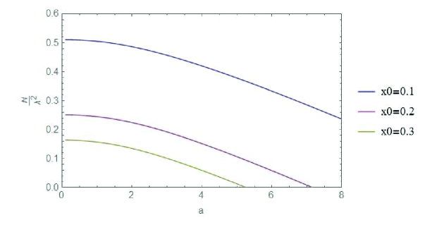
We obtained the numerical result as in Fig. 1
Figure 1: The graph for the negativity of the two detectors linearly coupled with the scalar field versus the acceleration (σ = 1 , Ω = 1 formulae-sequence 𝜎 1 Ω 1 \sigma=1,\Omega=1
It can be seen that the negativity decreases with the acceleration and comes to zero at a certain point. In addition, the entanglement decreases with the increase of the distance between the detectors, as anticipated.
4 Quadratic coupling
Now we consider two detectors which are quadratically coupled with a scalar field. The Hamiltonian in the interaction picture is
H = H A + H B , 𝐻 subscript 𝐻 𝐴 subscript 𝐻 𝐵 H=H_{A}+H_{B}, (48)
where
H j = λ j χ j ( τ ) ∫ Σ j N [ Φ ( τ , 𝐱 ) 2 ] [ f j ( 𝐱 ) σ j + e i Ω j τ + f j ( 𝐱 ) ∗ σ j − e − i Ω j τ ] − g d 3 𝐱 , subscript 𝐻 𝑗 subscript 𝜆 𝑗 subscript 𝜒 𝑗 𝜏 subscript subscript Σ 𝑗 𝑁 delimited-[] Φ superscript 𝜏 𝐱 2 delimited-[] subscript 𝑓 𝑗 𝐱 superscript subscript 𝜎 𝑗 superscript 𝑒 𝑖 subscript Ω 𝑗 𝜏 subscript 𝑓 𝑗 superscript 𝐱 superscript subscript 𝜎 𝑗 superscript 𝑒 𝑖 subscript Ω 𝑗 𝜏 𝑔 superscript 𝑑 3 𝐱 H_{j}=\lambda_{j}\chi_{j}(\tau)\int_{\Sigma_{j}}N\left[{\Phi}(\tau,\mathbf{x})^{2}\right]\left[f_{j}(\mathbf{x})\sigma_{j}^{+}e^{i\Omega_{j}\tau}+f_{j}(\mathbf{x})^{*}\sigma_{j}^{-}e^{-i\Omega_{j}\tau}\right]\sqrt{-g}d^{3}\mathbf{x}, (49)
j=A,B. Here we take the field operator to be Wick ordered to avoid potential divergences. There are two equivalent ways to realize Wick ordering, one being putting the creation operators to the left of the annihilation operators, the other one being taking the field to be the original one minus its vacuum expectation value. Both ways may cause ambiguity since the notion of mode expansion and the vacuum state is not uniquely defined in quantum field theory in curved spacetime. In this paper, we use the latter way.
In this way, the Wightman function for the quadratic coupling is related to the that for the linear coupling, which has been calculated in the last section.
The reduced density matrix shares the same structure with the case of Φ Φ {\Phi}
ρ = ( 1 − P A − P B 0 0 − M ∗ 0 P A L A B ∗ 0 0 L A B P B 0 − M 0 0 0 ) + o ( λ 2 ) , 𝜌 matrix 1 subscript 𝑃 𝐴 subscript 𝑃 𝐵 0 0 superscript 𝑀 0 subscript 𝑃 𝐴 superscript subscript 𝐿 𝐴 𝐵 0 0 subscript 𝐿 𝐴 𝐵 subscript 𝑃 𝐵 0 𝑀 0 0 0 𝑜 superscript 𝜆 2 \rho=\begin{pmatrix}1-P_{A}-P_{B}&0&0&-M^{*}\\
0&P_{A}&L_{AB}^{*}&0\\
0&L_{AB}&P_{B}&0\\
-M&0&0&0\end{pmatrix}+o(\lambda^{2}), (50)
where the matrix elements are
P j = subscript 𝑃 𝑗 absent \displaystyle P_{j}= λ j 2 ∫ 𝑑 τ 1 ∫ 𝑑 τ 2 χ j 1 χ j 2 e i Ω j ( τ 2 − τ 1 ) ∫ Σ j 2 − g 2 d 3 𝐱 2 f j 2 ∫ Σ j 1 − g 1 d 3 𝐱 1 f j 1 ∗ ⟨ 0 M | N ( Φ 1 2 ) N ( Φ 2 2 ) | 0 M ⟩ , j = A , B , formulae-sequence superscript subscript 𝜆 𝑗 2 differential-d subscript 𝜏 1 differential-d subscript 𝜏 2 subscript 𝜒 𝑗 1 subscript 𝜒 𝑗 2 superscript 𝑒 𝑖 subscript Ω 𝑗 subscript 𝜏 2 subscript 𝜏 1 subscript subscript Σ 𝑗 2 subscript 𝑔 2 superscript 𝑑 3 subscript 𝐱 2 subscript 𝑓 𝑗 2 subscript subscript Σ 𝑗 1 subscript 𝑔 1 superscript 𝑑 3 subscript 𝐱 1 superscript subscript 𝑓 𝑗 1 quantum-operator-product subscript 0 𝑀 𝑁 superscript subscript Φ 1 2 𝑁 superscript subscript Φ 2 2 subscript 0 𝑀 𝑗
𝐴 𝐵 \displaystyle\lambda_{j}^{2}\int d\tau_{1}\int d\tau_{2}\chi_{j1}\chi_{j2}e^{i\Omega_{j}(\tau_{2}-\tau_{1})}\int_{\Sigma_{j2}}\sqrt{-g_{2}}d^{3}\mathbf{x}_{2}f_{j2}\int_{\Sigma_{j1}}\sqrt{-g_{1}}d^{3}\mathbf{x}_{1}f_{j1}^{*}\langle 0_{M}|N\left({\Phi}_{1}^{2}\right)N\left({\Phi}_{2}^{2}\right)|0_{M}\rangle,j=A,B, (51)
L A B = subscript 𝐿 𝐴 𝐵 absent \displaystyle L_{AB}= λ A λ B ∫ 𝑑 τ 1 ∫ 𝑑 τ 2 χ A 1 χ B 2 e − i Ω A τ 1 + i Ω B τ 2 ∫ Σ A 1 − g 1 d 3 𝐱 1 f A 1 ∗ ∫ Σ B 2 − g 2 d 3 𝐱 2 f B 2 ⟨ 0 M | N ( Φ 1 2 ) N ( Φ 2 2 ) | 0 M ⟩ , subscript 𝜆 𝐴 subscript 𝜆 𝐵 differential-d subscript 𝜏 1 differential-d subscript 𝜏 2 subscript 𝜒 𝐴 1 subscript 𝜒 𝐵 2 superscript 𝑒 𝑖 subscript Ω 𝐴 subscript 𝜏 1 𝑖 subscript Ω 𝐵 subscript 𝜏 2 subscript subscript Σ 𝐴 1 subscript 𝑔 1 superscript 𝑑 3 subscript 𝐱 1 superscript subscript 𝑓 𝐴 1 subscript subscript Σ 𝐵 2 subscript 𝑔 2 superscript 𝑑 3 subscript 𝐱 2 subscript 𝑓 𝐵 2 quantum-operator-product subscript 0 𝑀 𝑁 superscript subscript Φ 1 2 𝑁 superscript subscript Φ 2 2 subscript 0 𝑀 \displaystyle\lambda_{A}\lambda_{B}\int d\tau_{1}\int d\tau_{2}\chi_{A1}\chi_{B2}e^{-i\Omega_{A}\tau_{1}+i\Omega_{B}\tau_{2}}\int_{\Sigma_{A1}}\sqrt{-g_{1}}d^{3}\mathbf{x}_{1}f_{A1}^{*}\int_{\Sigma_{B2}}\sqrt{-g_{2}}d^{3}\mathbf{x}_{2}f_{B2}\langle 0_{M}|N\left({\Phi}_{1}^{2}\right)N\left({\Phi}_{2}^{2}\right)|0_{M}\rangle, (52)
M = 𝑀 absent \displaystyle M= λ A λ B ∫ 𝑑 τ 1 ∫ 𝑑 τ 2 χ A 1 χ B 2 e i Ω A τ 1 + i Ω B τ 2 ∫ Σ A 1 f A 1 − g 1 d 3 𝐱 1 ∫ Σ B 2 f B 2 − g 2 d 3 𝐱 2 ⟨ 0 M | 𝒯 [ N ( Φ 1 2 ) N ( Φ 2 2 ) ] | 0 M ⟩ . subscript 𝜆 𝐴 subscript 𝜆 𝐵 differential-d subscript 𝜏 1 differential-d subscript 𝜏 2 subscript 𝜒 𝐴 1 subscript 𝜒 𝐵 2 superscript 𝑒 𝑖 subscript Ω 𝐴 subscript 𝜏 1 𝑖 subscript Ω 𝐵 subscript 𝜏 2 subscript subscript Σ 𝐴 1 subscript 𝑓 𝐴 1 subscript 𝑔 1 superscript 𝑑 3 subscript 𝐱 1 subscript subscript Σ 𝐵 2 subscript 𝑓 𝐵 2 subscript 𝑔 2 superscript 𝑑 3 subscript 𝐱 2 quantum-operator-product subscript 0 𝑀 𝒯 delimited-[] 𝑁 superscript subscript Φ 1 2 𝑁 superscript subscript Φ 2 2 subscript 0 𝑀 \displaystyle\lambda_{A}\lambda_{B}\int d\tau_{1}\int d\tau_{2}\chi_{A1}\chi_{B2}e^{i\Omega_{A}\tau_{1}+i\Omega_{B}\tau_{2}}\int_{\Sigma_{A1}}f_{A1}\sqrt{-g_{1}}d^{3}\mathbf{x}_{1}\int_{\Sigma_{B2}}f_{B2}\sqrt{-g_{2}}d^{3}\mathbf{x}_{2}\langle 0_{M}|\mathcal{T}\left[N\left({\Phi}_{1}^{2}\right)N\left({\Phi}_{2}^{2}\right)\right]|0_{M}\rangle. (53)
It should be clear now that we are to calculate the vacuum expectation value V Φ 2 subscript 𝑉 superscript Φ 2 V_{\Phi^{2}} 13
V Φ 2 = ⟨ 0 M | N ( Φ 1 2 ) N ( Φ 2 2 ) | 0 M ⟩ = 2 ⟨ 0 M | Φ 1 Φ 2 | 0 M ⟩ 2 = 2 ∫ 0 ∞ 𝑑 ω 1 ∫ 0 ∞ 𝑑 ω 2 ∬ d 2 𝐤 1 ⊥ ∬ d 2 𝐤 2 ⊥ 1 1 − e − 2 π ω 1 / a 1 1 − e − 2 π ω 2 / a × ( v 1 ω 1 𝐤 1 ⊥ R v 1 ω 2 𝐤 2 ⊥ R v 2 ω 1 𝐤 1 ⊥ R ∗ v 2 ω 2 𝐤 2 ⊥ R ∗ + v 1 ω 1 𝐤 1 ⊥ R v 1 ω 2 𝐤 2 ⊥ R ∗ v 2 ω 1 𝐤 1 ⊥ R ∗ v 2 ω 2 𝐤 2 ⊥ R e − 2 π ω 2 / a + v 1 ω 1 𝐤 1 ⊥ R ∗ v 1 ω 2 𝐤 2 ⊥ R v 2 ω 1 𝐤 1 ⊥ R v 2 ω 2 𝐤 2 ⊥ R ∗ e − 2 π ω 1 / a + v 1 ω 1 𝐤 1 ⊥ R ∗ v 1 ω 2 𝐤 2 ⊥ R ∗ v 2 ω 1 𝐤 1 ⊥ R v 2 ω 2 𝐤 2 ⊥ R e − 2 π ( ω 1 + ω 2 ) / a ) . subscript 𝑉 superscript Φ 2 quantum-operator-product subscript 0 𝑀 𝑁 superscript subscript Φ 1 2 𝑁 superscript subscript Φ 2 2 subscript 0 𝑀 2 superscript quantum-operator-product subscript 0 𝑀 subscript Φ 1 subscript Φ 2 subscript 0 𝑀 2 2 superscript subscript 0 differential-d subscript 𝜔 1 superscript subscript 0 differential-d subscript 𝜔 2 double-integral superscript 𝑑 2 subscript 𝐤 limit-from 1 bottom double-integral superscript 𝑑 2 subscript 𝐤 limit-from 2 bottom 1 1 superscript 𝑒 2 𝜋 subscript 𝜔 1 𝑎 1 1 superscript 𝑒 2 𝜋 subscript 𝜔 2 𝑎 subscript superscript 𝑣 𝑅 1 subscript 𝜔 1 subscript 𝐤 limit-from 1 bottom subscript superscript 𝑣 𝑅 1 subscript 𝜔 2 subscript 𝐤 limit-from 2 bottom subscript superscript 𝑣 𝑅
2 subscript 𝜔 1 subscript 𝐤 limit-from 1 bottom subscript superscript 𝑣 𝑅
2 subscript 𝜔 2 subscript 𝐤 limit-from 2 bottom subscript superscript 𝑣 𝑅 1 subscript 𝜔 1 subscript 𝐤 limit-from 1 bottom subscript superscript 𝑣 𝑅
1 subscript 𝜔 2 subscript 𝐤 limit-from 2 bottom subscript superscript 𝑣 𝑅
2 subscript 𝜔 1 subscript 𝐤 limit-from 1 bottom subscript superscript 𝑣 𝑅 2 subscript 𝜔 2 subscript 𝐤 limit-from 2 bottom superscript 𝑒 2 𝜋 subscript 𝜔 2 𝑎 subscript superscript 𝑣 𝑅
1 subscript 𝜔 1 subscript 𝐤 limit-from 1 bottom subscript superscript 𝑣 𝑅 1 subscript 𝜔 2 subscript 𝐤 limit-from 2 bottom subscript superscript 𝑣 𝑅 2 subscript 𝜔 1 subscript 𝐤 limit-from 1 bottom subscript superscript 𝑣 𝑅
2 subscript 𝜔 2 subscript 𝐤 limit-from 2 bottom superscript 𝑒 2 𝜋 subscript 𝜔 1 𝑎 subscript superscript 𝑣 𝑅
1 subscript 𝜔 1 subscript 𝐤 limit-from 1 bottom subscript superscript 𝑣 𝑅
1 subscript 𝜔 2 subscript 𝐤 limit-from 2 bottom subscript superscript 𝑣 𝑅 2 subscript 𝜔 1 subscript 𝐤 limit-from 1 bottom subscript superscript 𝑣 𝑅 2 subscript 𝜔 2 subscript 𝐤 limit-from 2 bottom superscript 𝑒 2 𝜋 subscript 𝜔 1 subscript 𝜔 2 𝑎 \begin{split}V_{\Phi^{2}}=&\langle 0_{M}|N\left({\Phi}_{1}^{2}\right)N\left({\Phi}_{2}^{2}\right)|0_{M}\rangle\\
=&2\langle 0_{M}|{\Phi}_{1}{\Phi}_{2}|0_{M}\rangle^{2}\\
=&2\int_{0}^{\infty}d\omega_{1}\int_{0}^{\infty}d\omega_{2}\iint d^{2}\mathbf{k}_{1\bot}\iint d^{2}\mathbf{k}_{2\bot}\frac{1}{1-e^{-2\pi\omega_{1}/a}}\frac{1}{1-e^{-2\pi\omega_{2}/a}}\\
&\times\left(v^{R}_{1\omega_{1}\mathbf{k}_{1\bot}}v^{R}_{1\omega_{2}\mathbf{k}_{2\bot}}v^{R*}_{2\omega_{1}\mathbf{k}_{1\bot}}v^{R*}_{2\omega_{2}\mathbf{k}_{2\bot}}+v^{R}_{1\omega_{1}\mathbf{k}_{1\bot}}v^{R*}_{1\omega_{2}\mathbf{k}_{2\bot}}v^{R*}_{2\omega_{1}\mathbf{k}_{1\bot}}v^{R}_{2\omega_{2}\mathbf{k}_{2\bot}}e^{-2\pi\omega_{2}/a}\right.\\
&\left.+v^{R*}_{1\omega_{1}\mathbf{k}_{1\bot}}v^{R}_{1\omega_{2}\mathbf{k}_{2\bot}}v^{R}_{2\omega_{1}\mathbf{k}_{1\bot}}v^{R*}_{2\omega_{2}\mathbf{k}_{2\bot}}e^{-2\pi\omega_{1}/a}+v^{R*}_{1\omega_{1}\mathbf{k}_{1\bot}}v^{R*}_{1\omega_{2}\mathbf{k}_{2\bot}}v^{R}_{2\omega_{1}\mathbf{k}_{1\bot}}v^{R}_{2\omega_{2}\mathbf{k}_{2\bot}}e^{-2\pi(\omega_{1}+\omega_{2})/a}\right).\end{split} (54)
Now it is a good time to make a digression to say a few words about the general structure of the interaction between detectors and quantum fields. The structure is well studied in Hummer-2016 M 𝑀 M 𝒯 [ e − i Ω ( τ 1 − τ 2 ) ] 𝒯 delimited-[] superscript 𝑒 𝑖 Ω subscript 𝜏 1 subscript 𝜏 2 \mathcal{T}\left[e^{-i\Omega(\tau_{1}-\tau_{2})}\right]
We follow the same procedure as in section 3 to calculate the matrix elements. The approach is the same but the calculation could be tedious so we leave the details in the Appendix and only describe the main steps and results.
4.1 Calculation of P j subscript 𝑃 𝑗 P_{j} L A B subscript 𝐿 𝐴 𝐵 L_{AB}
Let’s start with P j subscript 𝑃 𝑗 P_{j} L A B subscript 𝐿 𝐴 𝐵 L_{AB}
P j = 2 λ j 2 ∫ 0 ∞ 𝑑 ω 1 ∫ 0 ∞ 𝑑 ω 2 ∬ d 2 𝐤 1 ⊥ ∬ d 2 𝐤 2 ⊥ 1 1 − e − 2 π ω 1 / a 1 1 − e − 2 π ω 2 / a × ( | η ω 1 𝐤 1 ⊥ , ω 2 𝐤 2 ⊥ 0 j | 2 + | η ω 1 𝐤 1 ⊥ , ω 2 𝐤 2 ⊥ 2 j | 2 e − 2 π ω 2 / a + | η ω 1 𝐤 1 ⊥ , ω 2 𝐤 2 ⊥ 1 j | 2 e − 2 π ω 1 / a + | η ω 1 𝐤 1 ⊥ , ω 2 𝐤 2 ⊥ 12 j | 2 e − 2 π ( ω 1 + ω 2 ) / a ) , subscript 𝑃 𝑗 2 superscript subscript 𝜆 𝑗 2 superscript subscript 0 differential-d subscript 𝜔 1 superscript subscript 0 differential-d subscript 𝜔 2 double-integral superscript 𝑑 2 subscript 𝐤 limit-from 1 bottom double-integral superscript 𝑑 2 subscript 𝐤 limit-from 2 bottom 1 1 superscript 𝑒 2 𝜋 subscript 𝜔 1 𝑎 1 1 superscript 𝑒 2 𝜋 subscript 𝜔 2 𝑎 superscript subscript superscript 𝜂 0 𝑗 subscript 𝜔 1 subscript 𝐤 limit-from 1 bottom subscript 𝜔 2 subscript 𝐤 limit-from 2 bottom
2 superscript subscript superscript 𝜂 2 𝑗 subscript 𝜔 1 subscript 𝐤 limit-from 1 bottom subscript 𝜔 2 subscript 𝐤 limit-from 2 bottom
2 superscript 𝑒 2 𝜋 subscript 𝜔 2 𝑎 superscript subscript superscript 𝜂 1 𝑗 subscript 𝜔 1 subscript 𝐤 limit-from 1 bottom subscript 𝜔 2 subscript 𝐤 limit-from 2 bottom
2 superscript 𝑒 2 𝜋 subscript 𝜔 1 𝑎 superscript subscript superscript 𝜂 12 𝑗 subscript 𝜔 1 subscript 𝐤 limit-from 1 bottom subscript 𝜔 2 subscript 𝐤 limit-from 2 bottom
2 superscript 𝑒 2 𝜋 subscript 𝜔 1 subscript 𝜔 2 𝑎 \displaystyle\begin{split}P_{j}=&2\lambda_{j}^{2}\int_{0}^{\infty}d\omega_{1}\int_{0}^{\infty}d\omega_{2}\iint d^{2}\mathbf{k}_{1\bot}\iint d^{2}\mathbf{k}_{2\bot}\frac{1}{1-e^{-2\pi\omega_{1}/a}}\frac{1}{1-e^{-2\pi\omega_{2}/a}}\\
&\times\left(|\eta^{0j}_{\omega_{1}\mathbf{k}_{1\bot},\omega_{2}\mathbf{k}_{2\bot}}|^{2}+|\eta^{2j}_{\omega_{1}\mathbf{k}_{1\bot},\omega_{2}\mathbf{k}_{2\bot}}|^{2}e^{-2\pi\omega_{2}/a}+|\eta^{1j}_{\omega_{1}\mathbf{k}_{1\bot},\omega_{2}\mathbf{k}_{2\bot}}|^{2}e^{-2\pi\omega_{1}/a}+|\eta^{12j}_{\omega_{1}\mathbf{k}_{1\bot},\omega_{2}\mathbf{k}_{2\bot}}|^{2}e^{-2\pi(\omega_{1}+\omega_{2})/a}\right),\end{split} (55)
L A B = 2 λ A λ B ∫ 0 ∞ 𝑑 ω 1 ∫ 0 ∞ 𝑑 ω 2 ∬ d 2 𝐤 1 ⊥ ∬ d 2 𝐤 2 ⊥ 1 1 − e − 2 π ω 1 / a 1 1 − e − 2 π ω 2 / a × ( η ω 1 𝐤 1 ⊥ , ω 2 𝐤 2 ⊥ 0 A ∗ η ω 1 𝐤 1 ⊥ , ω 2 𝐤 2 ⊥ 0 B + η ω 1 𝐤 1 ⊥ , ω 2 𝐤 2 ⊥ 2 A ∗ η ω 1 𝐤 1 ⊥ , ω 2 𝐤 2 ⊥ 2 B e − 2 π ω 2 / a + η ω 1 𝐤 1 ⊥ , ω 2 𝐤 2 ⊥ 1 A ∗ η ω 1 𝐤 1 ⊥ , ω 2 𝐤 2 ⊥ 1 B e − 2 π ω 1 / a + η ω 1 𝐤 1 ⊥ , ω 2 𝐤 2 ⊥ 12 A ∗ η ω 1 𝐤 1 ⊥ , ω 2 𝐤 2 ⊥ 12 B e − 2 π ( ω 1 + ω 2 ) / a ) . subscript 𝐿 𝐴 𝐵 2 subscript 𝜆 𝐴 subscript 𝜆 𝐵 superscript subscript 0 differential-d subscript 𝜔 1 superscript subscript 0 differential-d subscript 𝜔 2 double-integral superscript 𝑑 2 subscript 𝐤 limit-from 1 bottom double-integral superscript 𝑑 2 subscript 𝐤 limit-from 2 bottom 1 1 superscript 𝑒 2 𝜋 subscript 𝜔 1 𝑎 1 1 superscript 𝑒 2 𝜋 subscript 𝜔 2 𝑎 subscript superscript 𝜂 0 𝐴
subscript 𝜔 1 subscript 𝐤 limit-from 1 bottom subscript 𝜔 2 subscript 𝐤 limit-from 2 bottom
subscript superscript 𝜂 0 𝐵 subscript 𝜔 1 subscript 𝐤 limit-from 1 bottom subscript 𝜔 2 subscript 𝐤 limit-from 2 bottom
subscript superscript 𝜂 2 𝐴
subscript 𝜔 1 subscript 𝐤 limit-from 1 bottom subscript 𝜔 2 subscript 𝐤 limit-from 2 bottom
subscript superscript 𝜂 2 𝐵 subscript 𝜔 1 subscript 𝐤 limit-from 1 bottom subscript 𝜔 2 subscript 𝐤 limit-from 2 bottom
superscript 𝑒 2 𝜋 subscript 𝜔 2 𝑎 subscript superscript 𝜂 1 𝐴
subscript 𝜔 1 subscript 𝐤 limit-from 1 bottom subscript 𝜔 2 subscript 𝐤 limit-from 2 bottom
subscript superscript 𝜂 1 𝐵 subscript 𝜔 1 subscript 𝐤 limit-from 1 bottom subscript 𝜔 2 subscript 𝐤 limit-from 2 bottom
superscript 𝑒 2 𝜋 subscript 𝜔 1 𝑎 subscript superscript 𝜂 12 𝐴
subscript 𝜔 1 subscript 𝐤 limit-from 1 bottom subscript 𝜔 2 subscript 𝐤 limit-from 2 bottom
subscript superscript 𝜂 12 𝐵 subscript 𝜔 1 subscript 𝐤 limit-from 1 bottom subscript 𝜔 2 subscript 𝐤 limit-from 2 bottom
superscript 𝑒 2 𝜋 subscript 𝜔 1 subscript 𝜔 2 𝑎 \displaystyle\begin{split}L_{AB}=&2\lambda_{A}\lambda_{B}\int_{0}^{\infty}d\omega_{1}\int_{0}^{\infty}d\omega_{2}\iint d^{2}\mathbf{k}_{1\bot}\iint d^{2}\mathbf{k}_{2\bot}\frac{1}{1-e^{-2\pi\omega_{1}/a}}\frac{1}{1-e^{-2\pi\omega_{2}/a}}\\
&\times\left(\eta^{0A*}_{\omega_{1}\mathbf{k}_{1\bot},\omega_{2}\mathbf{k}_{2\bot}}\eta^{0B}_{\omega_{1}\mathbf{k}_{1\bot},\omega_{2}\mathbf{k}_{2\bot}}+\eta^{2A*}_{\omega_{1}\mathbf{k}_{1\bot},\omega_{2}\mathbf{k}_{2\bot}}\eta^{2B}_{\omega_{1}\mathbf{k}_{1\bot},\omega_{2}\mathbf{k}_{2\bot}}e^{-2\pi\omega_{2}/a}+\eta^{1A*}_{\omega_{1}\mathbf{k}_{1\bot},\omega_{2}\mathbf{k}_{2\bot}}\eta^{1B}_{\omega_{1}\mathbf{k}_{1\bot},\omega_{2}\mathbf{k}_{2\bot}}e^{-2\pi\omega_{1}/a}\right.\\
&\left.+\eta^{12A*}_{\omega_{1}\mathbf{k}_{1\bot},\omega_{2}\mathbf{k}_{2\bot}}\eta^{12B}_{\omega_{1}\mathbf{k}_{1\bot},\omega_{2}\mathbf{k}_{2\bot}}e^{-2\pi(\omega_{1}+\omega_{2})/a}\right).\end{split} (56)
It is straightforward to write down the form of the η 𝜂 \eta
η ω 1 𝐤 1 ⊥ , ω 2 𝐤 2 ⊥ 0 = ∫ 𝑑 τ χ ( τ ) e i Ω τ ∫ Σ − g d 3 𝐱 f ( 𝐱 ) v ω 1 𝐤 1 ⊥ R ∗ v ω 2 𝐤 2 ⊥ R ∗ = ∫ 𝑑 τ 𝑑 ξ d 2 𝐱 ⊥ χ ( τ ) e 2 a ξ f ( ξ , 𝐱 ⊥ ) [ sinh ( π ω 1 / a ) 4 π 4 a ] 1 / 2 K i ω 1 / a ( κ 1 a e a ξ ) e − i 𝐤 1 ⊥ ⋅ 𝐱 ⊥ + i ω 1 τ × [ sinh ( π ω 2 / a ) 4 π 4 a ] 1 / 2 K i ω 2 / a ( κ 2 a e a ξ ) e − i 𝐤 2 ⊥ ⋅ 𝐱 ⊥ + i ω 2 τ e i Ω τ = ∫ 𝑑 τ 𝑑 ξ d 2 𝐱 ⊥ 1 2 π ∫ 𝑑 ν G ( ν ) e − i ν τ e 2 a ξ f ( ξ , 𝐱 ⊥ ) e − i ( 𝐤 1 ⊥ + 𝐤 2 ⊥ ) ⋅ 𝐱 ⊥ + i ( ω 1 + ω 2 + Ω ) τ × [ sinh ( π ω 1 / a ) 4 π 4 a ] 1 / 2 K i ω 1 / a ( κ 1 a e a ξ ) [ sinh ( π ω 2 / a ) 4 π 4 a ] 1 / 2 K i ω 2 / a ( κ 2 a e a ξ ) = 2 π 4 π 4 a ∫ 𝑑 ξ d 2 𝐱 ⊥ G ( ω 1 + ω 2 + Ω ) e 2 a ξ f ( ξ , 𝐱 ⊥ ) e − i ( 𝐤 1 ⊥ + 𝐤 2 ⊥ ) ⋅ 𝐱 ⊥ × sinh ( π ω 1 / a ) sinh ( π ω 2 / a ) K i ω 1 / a ( κ 1 a e a ξ ) K i ω 2 / a ( κ 2 a e a ξ ) . subscript superscript 𝜂 0 subscript 𝜔 1 subscript 𝐤 limit-from 1 bottom subscript 𝜔 2 subscript 𝐤 limit-from 2 bottom
differential-d 𝜏 𝜒 𝜏 superscript 𝑒 𝑖 Ω 𝜏 subscript Σ 𝑔 superscript 𝑑 3 𝐱 𝑓 𝐱 subscript superscript 𝑣 𝑅
subscript 𝜔 1 subscript 𝐤 limit-from 1 bottom subscript superscript 𝑣 𝑅
subscript 𝜔 2 subscript 𝐤 limit-from 2 bottom differential-d 𝜏 differential-d 𝜉 superscript 𝑑 2 subscript 𝐱 bottom 𝜒 𝜏 superscript 𝑒 2 𝑎 𝜉 𝑓 𝜉 subscript 𝐱 bottom superscript delimited-[] 𝜋 subscript 𝜔 1 𝑎 4 superscript 𝜋 4 𝑎 1 2 subscript 𝐾 𝑖 subscript 𝜔 1 𝑎 subscript 𝜅 1 𝑎 superscript 𝑒 𝑎 𝜉 superscript 𝑒 ⋅ 𝑖 subscript 𝐤 limit-from 1 bottom subscript 𝐱 bottom 𝑖 subscript 𝜔 1 𝜏 superscript delimited-[] 𝜋 subscript 𝜔 2 𝑎 4 superscript 𝜋 4 𝑎 1 2 subscript 𝐾 𝑖 subscript 𝜔 2 𝑎 subscript 𝜅 2 𝑎 superscript 𝑒 𝑎 𝜉 superscript 𝑒 ⋅ 𝑖 subscript 𝐤 limit-from 2 bottom subscript 𝐱 bottom 𝑖 subscript 𝜔 2 𝜏 superscript 𝑒 𝑖 Ω 𝜏 differential-d 𝜏 differential-d 𝜉 superscript 𝑑 2 subscript 𝐱 bottom 1 2 𝜋 differential-d 𝜈 𝐺 𝜈 superscript 𝑒 𝑖 𝜈 𝜏 superscript 𝑒 2 𝑎 𝜉 𝑓 𝜉 subscript 𝐱 bottom superscript 𝑒 ⋅ 𝑖 subscript 𝐤 limit-from 1 bottom subscript 𝐤 limit-from 2 bottom subscript 𝐱 bottom 𝑖 subscript 𝜔 1 subscript 𝜔 2 Ω 𝜏 superscript delimited-[] 𝜋 subscript 𝜔 1 𝑎 4 superscript 𝜋 4 𝑎 1 2 subscript 𝐾 𝑖 subscript 𝜔 1 𝑎 subscript 𝜅 1 𝑎 superscript 𝑒 𝑎 𝜉 superscript delimited-[] 𝜋 subscript 𝜔 2 𝑎 4 superscript 𝜋 4 𝑎 1 2 subscript 𝐾 𝑖 subscript 𝜔 2 𝑎 subscript 𝜅 2 𝑎 superscript 𝑒 𝑎 𝜉 2 𝜋 4 superscript 𝜋 4 𝑎 differential-d 𝜉 superscript 𝑑 2 subscript 𝐱 bottom 𝐺 subscript 𝜔 1 subscript 𝜔 2 Ω superscript 𝑒 2 𝑎 𝜉 𝑓 𝜉 subscript 𝐱 bottom superscript 𝑒 ⋅ 𝑖 subscript 𝐤 limit-from 1 bottom subscript 𝐤 limit-from 2 bottom subscript 𝐱 bottom 𝜋 subscript 𝜔 1 𝑎 𝜋 subscript 𝜔 2 𝑎 subscript 𝐾 𝑖 subscript 𝜔 1 𝑎 subscript 𝜅 1 𝑎 superscript 𝑒 𝑎 𝜉 subscript 𝐾 𝑖 subscript 𝜔 2 𝑎 subscript 𝜅 2 𝑎 superscript 𝑒 𝑎 𝜉 \begin{split}\eta^{0}_{\omega_{1}\mathbf{k}_{1\bot},\omega_{2}\mathbf{k}_{2\bot}}=&\int d\tau\chi(\tau)e^{i\Omega\tau}\int_{\Sigma}\sqrt{-g}d^{3}\mathbf{x}f(\mathbf{x})v^{R*}_{\omega_{1}\mathbf{k}_{1\bot}}v^{R*}_{\omega_{2}\mathbf{k}_{2\bot}}\\
=&\int d\tau d\xi d^{2}\mathbf{x}_{\bot}\chi(\tau)e^{2a\xi}f(\xi,\mathbf{x}_{\bot})\left[\frac{\sinh(\pi\omega_{1}/a)}{4\pi^{4}a}\right]^{1/2}K_{i\omega_{1}/a}\left(\frac{\kappa_{1}}{a}e^{a\xi}\right)e^{-i\mathbf{k}_{1\bot}\cdot\mathbf{x}_{\bot}+i\omega_{1}\tau}\\
&\times\left[\frac{\sinh(\pi\omega_{2}/a)}{4\pi^{4}a}\right]^{1/2}K_{i\omega_{2}/a}\left(\frac{\kappa_{2}}{a}e^{a\xi}\right)e^{-i\mathbf{k}_{2\bot}\cdot\mathbf{x}_{\bot}+i\omega_{2}\tau}e^{i\Omega\tau}\\
=&\int d\tau d\xi d^{2}\mathbf{x}_{\bot}\frac{1}{\sqrt{2\pi}}\int d\nu G(\nu)e^{-i\nu\tau}e^{2a\xi}f(\xi,\mathbf{x}_{\bot})e^{-i(\mathbf{k}_{1\bot}+\mathbf{k}_{2\bot})\cdot\mathbf{x}_{\bot}+i(\omega_{1}+\omega_{2}+\Omega)\tau}\\
&\times\left[\frac{\sinh(\pi\omega_{1}/a)}{4\pi^{4}a}\right]^{1/2}K_{i\omega_{1}/a}\left(\frac{\kappa_{1}}{a}e^{a\xi}\right)\left[\frac{\sinh(\pi\omega_{2}/a)}{4\pi^{4}a}\right]^{1/2}K_{i\omega_{2}/a}\left(\frac{\kappa_{2}}{a}e^{a\xi}\right)\\
=&\frac{\sqrt{2\pi}}{4\pi^{4}a}\int d\xi d^{2}\mathbf{x}_{\bot}G(\omega_{1}+\omega_{2}+\Omega)e^{2a\xi}f(\xi,\mathbf{x}_{\bot})e^{-i(\mathbf{k}_{1\bot}+\mathbf{k}_{2\bot})\cdot\mathbf{x}_{\bot}}\\
&\times\sqrt{\sinh(\pi\omega_{1}/a)\sinh(\pi\omega_{2}/a)}K_{i\omega_{1}/a}\left(\frac{\kappa_{1}}{a}e^{a\xi}\right)K_{i\omega_{2}/a}\left(\frac{\kappa_{2}}{a}e^{a\xi}\right).\end{split} (57)
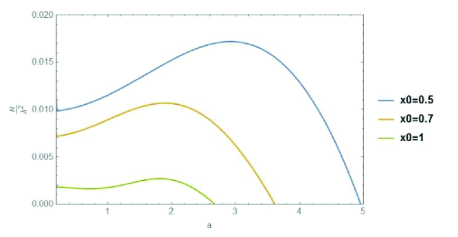
The final expression for the parameter values m = 0 , λ A = λ B = λ , Ω A = Ω B = Ω , σ A = σ B = σ , τ 0 = 0 , x 0 ≠ 0 formulae-sequence formulae-sequence 𝑚 0 subscript 𝜆 𝐴 subscript 𝜆 𝐵 𝜆 subscript Ω 𝐴 subscript Ω 𝐵 Ω subscript 𝜎 𝐴 subscript 𝜎 𝐵 𝜎 formulae-sequence subscript 𝜏 0 0 subscript 𝑥 0 0 m=0,\lambda_{A}=\lambda_{B}=\lambda,\Omega_{A}=\Omega_{B}=\Omega,\sigma_{A}=\sigma_{B}=\sigma,\tau_{0}=0,x_{0}\neq 0 M 𝑀 M
4.2 Calculation of M 𝑀 M
Now we calculate M 𝑀 M
D Φ 2 = ⟨ 0 M | 𝒯 [ N ( Φ 1 2 ) N ( Φ 2 2 ) ] | 0 M ⟩ = 2 θ ( τ 1 − τ 2 ) ⟨ 0 M | Φ ( τ 1 , 𝐱 1 ) Φ ( τ 2 , 𝐱 2 ) | 0 M ⟩ 2 + 2 θ ( τ 2 − τ 1 ) ⟨ 0 M | Φ ( τ 2 , 𝐱 2 ) Φ ( τ 1 , 𝐱 1 ) | 0 M ⟩ 2 = 2 ∫ 0 ∞ 𝑑 ω 1 ∫ 0 ∞ 𝑑 ω 2 ∬ d 2 𝐤 1 ⊥ ∬ d 2 𝐤 2 ⊥ 1 1 − e − 2 π ω 1 / a 1 1 − e − 2 π ω 2 / a × [ θ ( τ 1 − τ 2 ) ( v 1 ω 1 𝐤 1 ⊥ R v 1 ω 2 𝐤 2 ⊥ R v 2 ω 1 𝐤 1 ⊥ R ∗ v 2 ω 2 𝐤 2 ⊥ R ∗ + v 1 ω 1 𝐤 1 ⊥ R v 1 ω 2 𝐤 2 ⊥ R ∗ v 2 ω 1 𝐤 1 ⊥ R ∗ v 2 ω 2 𝐤 2 ⊥ R e − 2 π ω 2 / a + v 1 ω 1 𝐤 1 ⊥ R ∗ v 1 ω 2 𝐤 2 ⊥ R v 2 ω 1 𝐤 1 ⊥ R v 2 ω 2 𝐤 2 ⊥ R ∗ e − 2 π ω 1 / a + v 1 ω 1 𝐤 1 ⊥ R ∗ v 1 ω 2 𝐤 2 ⊥ R ∗ v 2 ω 1 𝐤 1 ⊥ R v 2 ω 2 𝐤 2 ⊥ R e − 2 π ( ω 1 + ω 2 ) / a ) + θ ( τ 2 − τ 1 ) ( v 2 ω 1 𝐤 1 ⊥ R v 2 ω 2 𝐤 2 ⊥ R v 1 ω 1 𝐤 1 ⊥ R ∗ v 1 ω 2 𝐤 2 ⊥ R ∗ + v 2 ω 1 𝐤 1 ⊥ R v 2 ω 2 𝐤 2 ⊥ R ∗ v 1 ω 1 𝐤 1 ⊥ R ∗ v 1 ω 2 𝐤 2 ⊥ R e − 2 π ω 2 / a + v 2 ω 1 𝐤 1 ⊥ R ∗ v 2 ω 2 𝐤 2 ⊥ R v 1 ω 1 𝐤 1 ⊥ R v 1 ω 2 𝐤 2 ⊥ R ∗ e − 2 π ω 1 / a + v 2 ω 1 𝐤 1 ⊥ R ∗ v 2 ω 2 𝐤 2 ⊥ R ∗ v 1 ω 1 𝐤 1 ⊥ R v 1 ω 2 𝐤 2 ⊥ R e − 2 π ( ω 1 + ω 2 ) / a ) ] . subscript 𝐷 superscript Φ 2 quantum-operator-product subscript 0 𝑀 𝒯 delimited-[] 𝑁 superscript subscript Φ 1 2 𝑁 superscript subscript Φ 2 2 subscript 0 𝑀 2 𝜃 subscript 𝜏 1 subscript 𝜏 2 superscript quantum-operator-product subscript 0 𝑀 Φ subscript 𝜏 1 subscript 𝐱 1 Φ subscript 𝜏 2 subscript 𝐱 2 subscript 0 𝑀 2 2 𝜃 subscript 𝜏 2 subscript 𝜏 1 superscript quantum-operator-product subscript 0 𝑀 Φ subscript 𝜏 2 subscript 𝐱 2 Φ subscript 𝜏 1 subscript 𝐱 1 subscript 0 𝑀 2 2 superscript subscript 0 differential-d subscript 𝜔 1 superscript subscript 0 differential-d subscript 𝜔 2 double-integral superscript 𝑑 2 subscript 𝐤 limit-from 1 bottom double-integral superscript 𝑑 2 subscript 𝐤 limit-from 2 bottom 1 1 superscript 𝑒 2 𝜋 subscript 𝜔 1 𝑎 1 1 superscript 𝑒 2 𝜋 subscript 𝜔 2 𝑎 delimited-[] 𝜃 subscript 𝜏 1 subscript 𝜏 2 subscript superscript 𝑣 𝑅 1 subscript 𝜔 1 subscript 𝐤 limit-from 1 bottom subscript superscript 𝑣 𝑅 1 subscript 𝜔 2 subscript 𝐤 limit-from 2 bottom subscript superscript 𝑣 𝑅
2 subscript 𝜔 1 subscript 𝐤 limit-from 1 bottom subscript superscript 𝑣 𝑅
2 subscript 𝜔 2 subscript 𝐤 limit-from 2 bottom subscript superscript 𝑣 𝑅 1 subscript 𝜔 1 subscript 𝐤 limit-from 1 bottom subscript superscript 𝑣 𝑅
1 subscript 𝜔 2 subscript 𝐤 limit-from 2 bottom subscript superscript 𝑣 𝑅
2 subscript 𝜔 1 subscript 𝐤 limit-from 1 bottom subscript superscript 𝑣 𝑅 2 subscript 𝜔 2 subscript 𝐤 limit-from 2 bottom superscript 𝑒 2 𝜋 subscript 𝜔 2 𝑎 subscript superscript 𝑣 𝑅
1 subscript 𝜔 1 subscript 𝐤 limit-from 1 bottom subscript superscript 𝑣 𝑅 1 subscript 𝜔 2 subscript 𝐤 limit-from 2 bottom subscript superscript 𝑣 𝑅 2 subscript 𝜔 1 subscript 𝐤 limit-from 1 bottom subscript superscript 𝑣 𝑅
2 subscript 𝜔 2 subscript 𝐤 limit-from 2 bottom superscript 𝑒 2 𝜋 subscript 𝜔 1 𝑎 subscript superscript 𝑣 𝑅
1 subscript 𝜔 1 subscript 𝐤 limit-from 1 bottom subscript superscript 𝑣 𝑅
1 subscript 𝜔 2 subscript 𝐤 limit-from 2 bottom subscript superscript 𝑣 𝑅 2 subscript 𝜔 1 subscript 𝐤 limit-from 1 bottom subscript superscript 𝑣 𝑅 2 subscript 𝜔 2 subscript 𝐤 limit-from 2 bottom superscript 𝑒 2 𝜋 subscript 𝜔 1 subscript 𝜔 2 𝑎 𝜃 subscript 𝜏 2 subscript 𝜏 1 subscript superscript 𝑣 𝑅 2 subscript 𝜔 1 subscript 𝐤 limit-from 1 bottom subscript superscript 𝑣 𝑅 2 subscript 𝜔 2 subscript 𝐤 limit-from 2 bottom subscript superscript 𝑣 𝑅
1 subscript 𝜔 1 subscript 𝐤 limit-from 1 bottom subscript superscript 𝑣 𝑅
1 subscript 𝜔 2 subscript 𝐤 limit-from 2 bottom subscript superscript 𝑣 𝑅 2 subscript 𝜔 1 subscript 𝐤 limit-from 1 bottom subscript superscript 𝑣 𝑅
2 subscript 𝜔 2 subscript 𝐤 limit-from 2 bottom subscript superscript 𝑣 𝑅
1 subscript 𝜔 1 subscript 𝐤 limit-from 1 bottom subscript superscript 𝑣 𝑅 1 subscript 𝜔 2 subscript 𝐤 limit-from 2 bottom superscript 𝑒 2 𝜋 subscript 𝜔 2 𝑎 subscript superscript 𝑣 𝑅
2 subscript 𝜔 1 subscript 𝐤 limit-from 1 bottom subscript superscript 𝑣 𝑅 2 subscript 𝜔 2 subscript 𝐤 limit-from 2 bottom subscript superscript 𝑣 𝑅 1 subscript 𝜔 1 subscript 𝐤 limit-from 1 bottom subscript superscript 𝑣 𝑅
1 subscript 𝜔 2 subscript 𝐤 limit-from 2 bottom superscript 𝑒 2 𝜋 subscript 𝜔 1 𝑎 subscript superscript 𝑣 𝑅
2 subscript 𝜔 1 subscript 𝐤 limit-from 1 bottom subscript superscript 𝑣 𝑅
2 subscript 𝜔 2 subscript 𝐤 limit-from 2 bottom subscript superscript 𝑣 𝑅 1 subscript 𝜔 1 subscript 𝐤 limit-from 1 bottom subscript superscript 𝑣 𝑅 1 subscript 𝜔 2 subscript 𝐤 limit-from 2 bottom superscript 𝑒 2 𝜋 subscript 𝜔 1 subscript 𝜔 2 𝑎 \begin{split}D_{\Phi^{2}}=&\langle 0_{M}|\mathcal{T}\left[N\left({\Phi}_{1}^{2}\right)N\left({\Phi}_{2}^{2}\right)\right]|0_{M}\rangle\\
=&2\theta(\tau_{1}-\tau_{2})\langle 0_{M}|{\Phi}(\tau_{1},\mathbf{x}_{1}){\Phi}(\tau_{2},\mathbf{x}_{2})|0_{M}\rangle^{2}+2\theta(\tau_{2}-\tau_{1})\langle 0_{M}|{\Phi}(\tau_{2},\mathbf{x}_{2}){\Phi}(\tau_{1},\mathbf{x}_{1})|0_{M}\rangle^{2}\\
=&2\int_{0}^{\infty}d\omega_{1}\int_{0}^{\infty}d\omega_{2}\iint d^{2}\mathbf{k}_{1\bot}\iint d^{2}\mathbf{k}_{2\bot}\frac{1}{1-e^{-2\pi\omega_{1}/a}}\frac{1}{1-e^{-2\pi\omega_{2}/a}}\\
&\times\left[\theta(\tau_{1}-\tau_{2})\left(v^{R}_{1\omega_{1}\mathbf{k}_{1\bot}}v^{R}_{1\omega_{2}\mathbf{k}_{2\bot}}v^{R*}_{2\omega_{1}\mathbf{k}_{1\bot}}v^{R*}_{2\omega_{2}\mathbf{k}_{2\bot}}+v^{R}_{1\omega_{1}\mathbf{k}_{1\bot}}v^{R*}_{1\omega_{2}\mathbf{k}_{2\bot}}v^{R*}_{2\omega_{1}\mathbf{k}_{1\bot}}v^{R}_{2\omega_{2}\mathbf{k}_{2\bot}}e^{-2\pi\omega_{2}/a}\right.\right.\\
&\left.+v^{R*}_{1\omega_{1}\mathbf{k}_{1\bot}}v^{R}_{1\omega_{2}\mathbf{k}_{2\bot}}v^{R}_{2\omega_{1}\mathbf{k}_{1\bot}}v^{R*}_{2\omega_{2}\mathbf{k}_{2\bot}}e^{-2\pi\omega_{1}/a}+v^{R*}_{1\omega_{1}\mathbf{k}_{1\bot}}v^{R*}_{1\omega_{2}\mathbf{k}_{2\bot}}v^{R}_{2\omega_{1}\mathbf{k}_{1\bot}}v^{R}_{2\omega_{2}\mathbf{k}_{2\bot}}e^{-2\pi(\omega_{1}+\omega_{2})/a}\right)\\
&+\theta(\tau_{2}-\tau_{1})\left(v^{R}_{2\omega_{1}\mathbf{k}_{1\bot}}v^{R}_{2\omega_{2}\mathbf{k}_{2\bot}}v^{R*}_{1\omega_{1}\mathbf{k}_{1\bot}}v^{R*}_{1\omega_{2}\mathbf{k}_{2\bot}}+v^{R}_{2\omega_{1}\mathbf{k}_{1\bot}}v^{R*}_{2\omega_{2}\mathbf{k}_{2\bot}}v^{R*}_{1\omega_{1}\mathbf{k}_{1\bot}}v^{R}_{1\omega_{2}\mathbf{k}_{2\bot}}e^{-2\pi\omega_{2}/a}\right.\\
&\left.\left.+v^{R*}_{2\omega_{1}\mathbf{k}_{1\bot}}v^{R}_{2\omega_{2}\mathbf{k}_{2\bot}}v^{R}_{1\omega_{1}\mathbf{k}_{1\bot}}v^{R*}_{1\omega_{2}\mathbf{k}_{2\bot}}e^{-2\pi\omega_{1}/a}+v^{R*}_{2\omega_{1}\mathbf{k}_{1\bot}}v^{R*}_{2\omega_{2}\mathbf{k}_{2\bot}}v^{R}_{1\omega_{1}\mathbf{k}_{1\bot}}v^{R}_{1\omega_{2}\mathbf{k}_{2\bot}}e^{-2\pi(\omega_{1}+\omega_{2})/a}\right)\right].\end{split} (58)
Substituting this expression into M 𝑀 M
M = 2 λ A λ B ∫ 𝑑 τ 1 ∫ 𝑑 τ 2 χ A 1 χ B 2 e i Ω A τ 1 + i Ω B τ 2 ∫ Σ A 1 f A 1 − g 1 d 3 𝐱 1 ∫ Σ B 2 f B 2 − g 2 d 3 𝐱 2 ∫ 0 ∞ 𝑑 ω 1 ∫ 0 ∞ 𝑑 ω 2 ∬ d 2 𝐤 1 ⊥ ∬ d 2 𝐤 2 ⊥ 1 1 − e − 2 π ω 1 / a 1 1 − e − 2 π ω 2 / a × [ θ ( τ 1 − τ 2 ) ( v 1 ω 1 𝐤 1 ⊥ R v 1 ω 2 𝐤 2 ⊥ R v 2 ω 1 𝐤 1 ⊥ R ∗ v 2 ω 2 𝐤 2 ⊥ R ∗ + v 1 ω 1 𝐤 1 ⊥ R v 1 ω 2 𝐤 2 ⊥ R ∗ v 2 ω 1 𝐤 1 ⊥ R ∗ v 2 ω 2 𝐤 2 ⊥ R e − 2 π ω 2 / a + v 1 ω 1 𝐤 1 ⊥ R ∗ v 1 ω 2 𝐤 2 ⊥ R v 2 ω 1 𝐤 1 ⊥ R v 2 ω 2 𝐤 2 ⊥ R ∗ e − 2 π ω 1 / a + v 1 ω 1 𝐤 1 ⊥ R ∗ v 1 ω 2 𝐤 2 ⊥ R ∗ v 2 ω 1 𝐤 1 ⊥ R v 2 ω 2 𝐤 2 ⊥ R e − 2 π ( ω 1 + ω 2 ) / a ) + θ ( τ 2 − τ 1 ) ( v 2 ω 1 𝐤 1 ⊥ R v 2 ω 2 𝐤 2 ⊥ R v 1 ω 1 𝐤 1 ⊥ R ∗ v 1 ω 2 𝐤 2 ⊥ R ∗ + v 2 ω 1 𝐤 1 ⊥ R v 2 ω 2 𝐤 2 ⊥ R ∗ v 1 ω 1 𝐤 1 ⊥ R ∗ v 1 ω 2 𝐤 2 ⊥ R e − 2 π ω 2 / a + v 2 ω 1 𝐤 1 ⊥ R ∗ v 2 ω 2 𝐤 2 ⊥ R v 1 ω 1 𝐤 1 ⊥ R v 1 ω 2 𝐤 2 ⊥ R ∗ e − 2 π ω 1 / a + v 2 ω 1 𝐤 1 ⊥ R ∗ v 2 ω 2 𝐤 2 ⊥ R ∗ v 1 ω 1 𝐤 1 ⊥ R v 1 ω 2 𝐤 2 ⊥ R e − 2 π ( ω 1 + ω 2 ) / a ) ] = 2 λ A λ B ∫ 0 ∞ 𝑑 ω 1 ∫ 0 ∞ 𝑑 ω 2 ∬ d 2 𝐤 1 ⊥ ∬ d 2 𝐤 2 ⊥ 1 1 − e − 2 π ω 1 / a 1 1 − e − 2 π ω 2 / a × [ W ω 1 𝐤 1 ⊥ , ω 2 𝐤 2 ⊥ 0 + W ω 1 𝐤 1 ⊥ , ω 2 𝐤 2 ⊥ 2 e − 2 π ω 2 / a + W ω 1 𝐤 1 ⊥ , ω 2 𝐤 2 ⊥ 1 e − 2 π ω 1 / a + W ω 1 𝐤 1 ⊥ , ω 2 𝐤 2 ⊥ 12 e − 2 π ( ω 1 + ω 2 ) / a ] . 𝑀 2 subscript 𝜆 𝐴 subscript 𝜆 𝐵 differential-d subscript 𝜏 1 differential-d subscript 𝜏 2 subscript 𝜒 𝐴 1 subscript 𝜒 𝐵 2 superscript 𝑒 𝑖 subscript Ω 𝐴 subscript 𝜏 1 𝑖 subscript Ω 𝐵 subscript 𝜏 2 subscript subscript Σ 𝐴 1 subscript 𝑓 𝐴 1 subscript 𝑔 1 superscript 𝑑 3 subscript 𝐱 1 subscript subscript Σ 𝐵 2 subscript 𝑓 𝐵 2 subscript 𝑔 2 superscript 𝑑 3 subscript 𝐱 2 superscript subscript 0 differential-d subscript 𝜔 1 superscript subscript 0 differential-d subscript 𝜔 2 double-integral superscript 𝑑 2 subscript 𝐤 limit-from 1 bottom double-integral superscript 𝑑 2 subscript 𝐤 limit-from 2 bottom 1 1 superscript 𝑒 2 𝜋 subscript 𝜔 1 𝑎 1 1 superscript 𝑒 2 𝜋 subscript 𝜔 2 𝑎 delimited-[] 𝜃 subscript 𝜏 1 subscript 𝜏 2 subscript superscript 𝑣 𝑅 1 subscript 𝜔 1 subscript 𝐤 limit-from 1 bottom subscript superscript 𝑣 𝑅 1 subscript 𝜔 2 subscript 𝐤 limit-from 2 bottom subscript superscript 𝑣 𝑅
2 subscript 𝜔 1 subscript 𝐤 limit-from 1 bottom subscript superscript 𝑣 𝑅
2 subscript 𝜔 2 subscript 𝐤 limit-from 2 bottom subscript superscript 𝑣 𝑅 1 subscript 𝜔 1 subscript 𝐤 limit-from 1 bottom subscript superscript 𝑣 𝑅
1 subscript 𝜔 2 subscript 𝐤 limit-from 2 bottom subscript superscript 𝑣 𝑅
2 subscript 𝜔 1 subscript 𝐤 limit-from 1 bottom subscript superscript 𝑣 𝑅 2 subscript 𝜔 2 subscript 𝐤 limit-from 2 bottom superscript 𝑒 2 𝜋 subscript 𝜔 2 𝑎 subscript superscript 𝑣 𝑅
1 subscript 𝜔 1 subscript 𝐤 limit-from 1 bottom subscript superscript 𝑣 𝑅 1 subscript 𝜔 2 subscript 𝐤 limit-from 2 bottom subscript superscript 𝑣 𝑅 2 subscript 𝜔 1 subscript 𝐤 limit-from 1 bottom subscript superscript 𝑣 𝑅
2 subscript 𝜔 2 subscript 𝐤 limit-from 2 bottom superscript 𝑒 2 𝜋 subscript 𝜔 1 𝑎 subscript superscript 𝑣 𝑅
1 subscript 𝜔 1 subscript 𝐤 limit-from 1 bottom subscript superscript 𝑣 𝑅
1 subscript 𝜔 2 subscript 𝐤 limit-from 2 bottom subscript superscript 𝑣 𝑅 2 subscript 𝜔 1 subscript 𝐤 limit-from 1 bottom subscript superscript 𝑣 𝑅 2 subscript 𝜔 2 subscript 𝐤 limit-from 2 bottom superscript 𝑒 2 𝜋 subscript 𝜔 1 subscript 𝜔 2 𝑎 𝜃 subscript 𝜏 2 subscript 𝜏 1 subscript superscript 𝑣 𝑅 2 subscript 𝜔 1 subscript 𝐤 limit-from 1 bottom subscript superscript 𝑣 𝑅 2 subscript 𝜔 2 subscript 𝐤 limit-from 2 bottom subscript superscript 𝑣 𝑅
1 subscript 𝜔 1 subscript 𝐤 limit-from 1 bottom subscript superscript 𝑣 𝑅
1 subscript 𝜔 2 subscript 𝐤 limit-from 2 bottom subscript superscript 𝑣 𝑅 2 subscript 𝜔 1 subscript 𝐤 limit-from 1 bottom subscript superscript 𝑣 𝑅
2 subscript 𝜔 2 subscript 𝐤 limit-from 2 bottom subscript superscript 𝑣 𝑅
1 subscript 𝜔 1 subscript 𝐤 limit-from 1 bottom subscript superscript 𝑣 𝑅 1 subscript 𝜔 2 subscript 𝐤 limit-from 2 bottom superscript 𝑒 2 𝜋 subscript 𝜔 2 𝑎 subscript superscript 𝑣 𝑅
2 subscript 𝜔 1 subscript 𝐤 limit-from 1 bottom subscript superscript 𝑣 𝑅 2 subscript 𝜔 2 subscript 𝐤 limit-from 2 bottom subscript superscript 𝑣 𝑅 1 subscript 𝜔 1 subscript 𝐤 limit-from 1 bottom subscript superscript 𝑣 𝑅
1 subscript 𝜔 2 subscript 𝐤 limit-from 2 bottom superscript 𝑒 2 𝜋 subscript 𝜔 1 𝑎 subscript superscript 𝑣 𝑅
2 subscript 𝜔 1 subscript 𝐤 limit-from 1 bottom subscript superscript 𝑣 𝑅
2 subscript 𝜔 2 subscript 𝐤 limit-from 2 bottom subscript superscript 𝑣 𝑅 1 subscript 𝜔 1 subscript 𝐤 limit-from 1 bottom subscript superscript 𝑣 𝑅 1 subscript 𝜔 2 subscript 𝐤 limit-from 2 bottom superscript 𝑒 2 𝜋 subscript 𝜔 1 subscript 𝜔 2 𝑎 2 subscript 𝜆 𝐴 subscript 𝜆 𝐵 superscript subscript 0 differential-d subscript 𝜔 1 superscript subscript 0 differential-d subscript 𝜔 2 double-integral superscript 𝑑 2 subscript 𝐤 limit-from 1 bottom double-integral superscript 𝑑 2 subscript 𝐤 limit-from 2 bottom 1 1 superscript 𝑒 2 𝜋 subscript 𝜔 1 𝑎 1 1 superscript 𝑒 2 𝜋 subscript 𝜔 2 𝑎 delimited-[] subscript superscript 𝑊 0 subscript 𝜔 1 subscript 𝐤 limit-from 1 bottom subscript 𝜔 2 subscript 𝐤 limit-from 2 bottom
subscript superscript 𝑊 2 subscript 𝜔 1 subscript 𝐤 limit-from 1 bottom subscript 𝜔 2 subscript 𝐤 limit-from 2 bottom
superscript 𝑒 2 𝜋 subscript 𝜔 2 𝑎 subscript superscript 𝑊 1 subscript 𝜔 1 subscript 𝐤 limit-from 1 bottom subscript 𝜔 2 subscript 𝐤 limit-from 2 bottom
superscript 𝑒 2 𝜋 subscript 𝜔 1 𝑎 subscript superscript 𝑊 12 subscript 𝜔 1 subscript 𝐤 limit-from 1 bottom subscript 𝜔 2 subscript 𝐤 limit-from 2 bottom
superscript 𝑒 2 𝜋 subscript 𝜔 1 subscript 𝜔 2 𝑎 \begin{split}M=&2\lambda_{A}\lambda_{B}\int d\tau_{1}\int d\tau_{2}\chi_{A1}\chi_{B2}e^{i\Omega_{A}\tau_{1}+i\Omega_{B}\tau_{2}}\int_{\Sigma_{A1}}f_{A1}\sqrt{-g_{1}}d^{3}\mathbf{x}_{1}\int_{\Sigma_{B2}}f_{B2}\sqrt{-g_{2}}d^{3}\mathbf{x}_{2}\\
&\int_{0}^{\infty}d\omega_{1}\int_{0}^{\infty}d\omega_{2}\iint d^{2}\mathbf{k}_{1\bot}\iint d^{2}\mathbf{k}_{2\bot}\frac{1}{1-e^{-2\pi\omega_{1}/a}}\frac{1}{1-e^{-2\pi\omega_{2}/a}}\\
&\times\left[\theta(\tau_{1}-\tau_{2})\left(v^{R}_{1\omega_{1}\mathbf{k}_{1\bot}}v^{R}_{1\omega_{2}\mathbf{k}_{2\bot}}v^{R*}_{2\omega_{1}\mathbf{k}_{1\bot}}v^{R*}_{2\omega_{2}\mathbf{k}_{2\bot}}+v^{R}_{1\omega_{1}\mathbf{k}_{1\bot}}v^{R*}_{1\omega_{2}\mathbf{k}_{2\bot}}v^{R*}_{2\omega_{1}\mathbf{k}_{1\bot}}v^{R}_{2\omega_{2}\mathbf{k}_{2\bot}}e^{-2\pi\omega_{2}/a}\right.\right.\\
&\left.+v^{R*}_{1\omega_{1}\mathbf{k}_{1\bot}}v^{R}_{1\omega_{2}\mathbf{k}_{2\bot}}v^{R}_{2\omega_{1}\mathbf{k}_{1\bot}}v^{R*}_{2\omega_{2}\mathbf{k}_{2\bot}}e^{-2\pi\omega_{1}/a}+v^{R*}_{1\omega_{1}\mathbf{k}_{1\bot}}v^{R*}_{1\omega_{2}\mathbf{k}_{2\bot}}v^{R}_{2\omega_{1}\mathbf{k}_{1\bot}}v^{R}_{2\omega_{2}\mathbf{k}_{2\bot}}e^{-2\pi(\omega_{1}+\omega_{2})/a}\right)\\
&+\theta(\tau_{2}-\tau_{1})\left(v^{R}_{2\omega_{1}\mathbf{k}_{1\bot}}v^{R}_{2\omega_{2}\mathbf{k}_{2\bot}}v^{R*}_{1\omega_{1}\mathbf{k}_{1\bot}}v^{R*}_{1\omega_{2}\mathbf{k}_{2\bot}}+v^{R}_{2\omega_{1}\mathbf{k}_{1\bot}}v^{R*}_{2\omega_{2}\mathbf{k}_{2\bot}}v^{R*}_{1\omega_{1}\mathbf{k}_{1\bot}}v^{R}_{1\omega_{2}\mathbf{k}_{2\bot}}e^{-2\pi\omega_{2}/a}\right.\\
&\left.\left.+v^{R*}_{2\omega_{1}\mathbf{k}_{1\bot}}v^{R}_{2\omega_{2}\mathbf{k}_{2\bot}}v^{R}_{1\omega_{1}\mathbf{k}_{1\bot}}v^{R*}_{1\omega_{2}\mathbf{k}_{2\bot}}e^{-2\pi\omega_{1}/a}+v^{R*}_{2\omega_{1}\mathbf{k}_{1\bot}}v^{R*}_{2\omega_{2}\mathbf{k}_{2\bot}}v^{R}_{1\omega_{1}\mathbf{k}_{1\bot}}v^{R}_{1\omega_{2}\mathbf{k}_{2\bot}}e^{-2\pi(\omega_{1}+\omega_{2})/a}\right)\right]\\
=&2\lambda_{A}\lambda_{B}\int_{0}^{\infty}d\omega_{1}\int_{0}^{\infty}d\omega_{2}\iint d^{2}\mathbf{k}_{1\bot}\iint d^{2}\mathbf{k}_{2\bot}\frac{1}{1-e^{-2\pi\omega_{1}/a}}\frac{1}{1-e^{-2\pi\omega_{2}/a}}\\
&\times\left[W^{0}_{\omega_{1}\mathbf{k}_{1\bot},\omega_{2}\mathbf{k}_{2\bot}}+W^{2}_{\omega_{1}\mathbf{k}_{1\bot},\omega_{2}\mathbf{k}_{2\bot}}e^{-2\pi\omega_{2}/a}+W^{1}_{\omega_{1}\mathbf{k}_{1\bot},\omega_{2}\mathbf{k}_{2\bot}}e^{-2\pi\omega_{1}/a}+W^{12}_{\omega_{1}\mathbf{k}_{1\bot},\omega_{2}\mathbf{k}_{2\bot}}e^{-2\pi(\omega_{1}+\omega_{2})/a}\right].\end{split} (59)
These terms looks complicated but can be calculated straightforwardly. Here we take W ω 1 𝐤 1 ⊥ , ω 2 𝐤 2 ⊥ 0 subscript superscript 𝑊 0 subscript 𝜔 1 subscript 𝐤 limit-from 1 bottom subscript 𝜔 2 subscript 𝐤 limit-from 2 bottom
W^{0}_{\omega_{1}\mathbf{k}_{1\bot},\omega_{2}\mathbf{k}_{2\bot}}
W ω 1 𝐤 1 ⊥ , ω 2 𝐤 2 ⊥ 0 = subscript superscript 𝑊 0 subscript 𝜔 1 subscript 𝐤 limit-from 1 bottom subscript 𝜔 2 subscript 𝐤 limit-from 2 bottom
absent \displaystyle W^{0}_{\omega_{1}\mathbf{k}_{1\bot},\omega_{2}\mathbf{k}_{2\bot}}= ∫ 𝑑 τ 1 ∫ 𝑑 τ 2 χ A 1 χ B 2 e i Ω A τ 1 + i Ω B τ 2 ∫ Σ A 1 f A 1 − g 1 d 3 𝐱 1 ∫ Σ B 2 f B 2 − g 2 d 3 𝐱 2 differential-d subscript 𝜏 1 differential-d subscript 𝜏 2 subscript 𝜒 𝐴 1 subscript 𝜒 𝐵 2 superscript 𝑒 𝑖 subscript Ω 𝐴 subscript 𝜏 1 𝑖 subscript Ω 𝐵 subscript 𝜏 2 subscript subscript Σ 𝐴 1 subscript 𝑓 𝐴 1 subscript 𝑔 1 superscript 𝑑 3 subscript 𝐱 1 subscript subscript Σ 𝐵 2 subscript 𝑓 𝐵 2 subscript 𝑔 2 superscript 𝑑 3 subscript 𝐱 2 \displaystyle\int d\tau_{1}\int d\tau_{2}\chi_{A1}\chi_{B2}e^{i\Omega_{A}\tau_{1}+i\Omega_{B}\tau_{2}}\int_{\Sigma_{A1}}f_{A1}\sqrt{-g_{1}}d^{3}\mathbf{x}_{1}\int_{\Sigma_{B2}}f_{B2}\sqrt{-g_{2}}d^{3}\mathbf{x}_{2}
× [ θ ( τ 1 − τ 2 ) v 1 ω 1 𝐤 1 ⊥ R v 1 ω 2 𝐤 2 ⊥ R v 2 ω 1 𝐤 1 ⊥ R ∗ v 2 ω 2 𝐤 2 ⊥ R ∗ + θ ( τ 2 − τ 1 ) v 2 ω 1 𝐤 1 ⊥ R v 2 ω 2 𝐤 2 ⊥ R v 1 ω 1 𝐤 1 ⊥ R ∗ v 1 ω 2 𝐤 2 ⊥ R ∗ ] absent delimited-[] 𝜃 subscript 𝜏 1 subscript 𝜏 2 subscript superscript 𝑣 𝑅 1 subscript 𝜔 1 subscript 𝐤 limit-from 1 bottom subscript superscript 𝑣 𝑅 1 subscript 𝜔 2 subscript 𝐤 limit-from 2 bottom subscript superscript 𝑣 𝑅
2 subscript 𝜔 1 subscript 𝐤 limit-from 1 bottom subscript superscript 𝑣 𝑅
2 subscript 𝜔 2 subscript 𝐤 limit-from 2 bottom 𝜃 subscript 𝜏 2 subscript 𝜏 1 subscript superscript 𝑣 𝑅 2 subscript 𝜔 1 subscript 𝐤 limit-from 1 bottom subscript superscript 𝑣 𝑅 2 subscript 𝜔 2 subscript 𝐤 limit-from 2 bottom subscript superscript 𝑣 𝑅
1 subscript 𝜔 1 subscript 𝐤 limit-from 1 bottom subscript superscript 𝑣 𝑅
1 subscript 𝜔 2 subscript 𝐤 limit-from 2 bottom \displaystyle\times\left[\theta(\tau_{1}-\tau_{2})v^{R}_{1\omega_{1}\mathbf{k}_{1\bot}}v^{R}_{1\omega_{2}\mathbf{k}_{2\bot}}v^{R*}_{2\omega_{1}\mathbf{k}_{1\bot}}v^{R*}_{2\omega_{2}\mathbf{k}_{2\bot}}+\theta(\tau_{2}-\tau_{1})v^{R}_{2\omega_{1}\mathbf{k}_{1\bot}}v^{R}_{2\omega_{2}\mathbf{k}_{2\bot}}v^{R*}_{1\omega_{1}\mathbf{k}_{1\bot}}v^{R*}_{1\omega_{2}\mathbf{k}_{2\bot}}\right]
= \displaystyle= sinh ( π ω 1 / a ) sinh ( π ω 2 / a ) ( 4 π 4 a ) 2 ∫ 𝑑 τ 1 ∫ 𝑑 τ 2 χ A 1 χ B 2 e i Ω A τ 1 + i Ω B τ 2 ∫ Σ A 1 f A 1 − g 1 d 3 𝐱 1 ∫ Σ B 2 f B 2 − g 2 d 3 𝐱 2 𝜋 subscript 𝜔 1 𝑎 𝜋 subscript 𝜔 2 𝑎 superscript 4 superscript 𝜋 4 𝑎 2 differential-d subscript 𝜏 1 differential-d subscript 𝜏 2 subscript 𝜒 𝐴 1 subscript 𝜒 𝐵 2 superscript 𝑒 𝑖 subscript Ω 𝐴 subscript 𝜏 1 𝑖 subscript Ω 𝐵 subscript 𝜏 2 subscript subscript Σ 𝐴 1 subscript 𝑓 𝐴 1 subscript 𝑔 1 superscript 𝑑 3 subscript 𝐱 1 subscript subscript Σ 𝐵 2 subscript 𝑓 𝐵 2 subscript 𝑔 2 superscript 𝑑 3 subscript 𝐱 2 \displaystyle\frac{\sinh(\pi\omega_{1}/a)\sinh(\pi\omega_{2}/a)}{(4\pi^{4}a)^{2}}\int d\tau_{1}\int d\tau_{2}\chi_{A1}\chi_{B2}e^{i\Omega_{A}\tau_{1}+i\Omega_{B}\tau_{2}}\int_{\Sigma_{A1}}f_{A1}\sqrt{-g_{1}}d^{3}\mathbf{x}_{1}\int_{\Sigma_{B2}}f_{B2}\sqrt{-g_{2}}d^{3}\mathbf{x}_{2}
× K i ω 1 / a ( κ 1 a e a ξ 1 ) K i ω 2 / a ( κ 2 a e a ξ 1 ) K i ω 1 / a ( κ 1 a e a ξ 2 ) K i ω 2 / a ( κ 2 a e a ξ 2 ) absent subscript 𝐾 𝑖 subscript 𝜔 1 𝑎 subscript 𝜅 1 𝑎 superscript 𝑒 𝑎 subscript 𝜉 1 subscript 𝐾 𝑖 subscript 𝜔 2 𝑎 subscript 𝜅 2 𝑎 superscript 𝑒 𝑎 subscript 𝜉 1 subscript 𝐾 𝑖 subscript 𝜔 1 𝑎 subscript 𝜅 1 𝑎 superscript 𝑒 𝑎 subscript 𝜉 2 subscript 𝐾 𝑖 subscript 𝜔 2 𝑎 subscript 𝜅 2 𝑎 superscript 𝑒 𝑎 subscript 𝜉 2 \displaystyle\times K_{i\omega_{1}/a}\left(\frac{\kappa_{1}}{a}e^{a\xi_{1}}\right)K_{i\omega_{2}/a}\left(\frac{\kappa_{2}}{a}e^{a\xi_{1}}\right)K_{i\omega_{1}/a}\left(\frac{\kappa_{1}}{a}e^{a\xi_{2}}\right)K_{i\omega_{2}/a}\left(\frac{\kappa_{2}}{a}e^{a\xi_{2}}\right)
× [ θ ( τ 1 − τ 2 ) e i ( 𝐤 1 ⊥ + 𝐤 2 ⊥ ) ⋅ ( 𝐱 1 ⊥ − 𝐱 2 ⊥ ) − i ( ω 1 + ω 2 ) ( τ 1 − τ 2 ) + θ ( τ 2 − τ 1 ) e − i ( 𝐤 1 ⊥ + 𝐤 2 ⊥ ) ⋅ ( 𝐱 1 ⊥ − 𝐱 2 ⊥ ) + i ( ω 1 + ω 2 ) ( τ 1 − τ 2 ) ] absent delimited-[] 𝜃 subscript 𝜏 1 subscript 𝜏 2 superscript 𝑒 ⋅ 𝑖 subscript 𝐤 limit-from 1 bottom subscript 𝐤 limit-from 2 bottom subscript 𝐱 limit-from 1 bottom subscript 𝐱 limit-from 2 bottom 𝑖 subscript 𝜔 1 subscript 𝜔 2 subscript 𝜏 1 subscript 𝜏 2 𝜃 subscript 𝜏 2 subscript 𝜏 1 superscript 𝑒 ⋅ 𝑖 subscript 𝐤 limit-from 1 bottom subscript 𝐤 limit-from 2 bottom subscript 𝐱 limit-from 1 bottom subscript 𝐱 limit-from 2 bottom 𝑖 subscript 𝜔 1 subscript 𝜔 2 subscript 𝜏 1 subscript 𝜏 2 \displaystyle\times\left[\theta(\tau_{1}-\tau_{2})e^{i(\mathbf{k}_{1\bot}+\mathbf{k}_{2\bot})\cdot(\mathbf{x}_{1\bot}-\mathbf{x}_{2\bot})-i(\omega_{1}+\omega_{2})(\tau_{1}-\tau_{2})}+\theta(\tau_{2}-\tau_{1})e^{-i(\mathbf{k}_{1\bot}+\mathbf{k}_{2\bot})\cdot(\mathbf{x}_{1\bot}-\mathbf{x}_{2\bot})+i(\omega_{1}+\omega_{2})(\tau_{1}-\tau_{2})}\right]
= \displaystyle= sinh ( π ω 1 / a ) sinh ( π ω 2 / a ) ( 4 π 4 a ) 2 ∫ 𝑑 τ 1 ∫ 𝑑 τ 2 χ A 1 χ B 2 e i Ω A τ 1 + i Ω B τ 2 ∫ Σ A 1 f A 1 − g 1 d 3 𝐱 1 ∫ Σ B 2 f B 2 − g 2 d 3 𝐱 2 𝜋 subscript 𝜔 1 𝑎 𝜋 subscript 𝜔 2 𝑎 superscript 4 superscript 𝜋 4 𝑎 2 differential-d subscript 𝜏 1 differential-d subscript 𝜏 2 subscript 𝜒 𝐴 1 subscript 𝜒 𝐵 2 superscript 𝑒 𝑖 subscript Ω 𝐴 subscript 𝜏 1 𝑖 subscript Ω 𝐵 subscript 𝜏 2 subscript subscript Σ 𝐴 1 subscript 𝑓 𝐴 1 subscript 𝑔 1 superscript 𝑑 3 subscript 𝐱 1 subscript subscript Σ 𝐵 2 subscript 𝑓 𝐵 2 subscript 𝑔 2 superscript 𝑑 3 subscript 𝐱 2 \displaystyle\frac{\sinh(\pi\omega_{1}/a)\sinh(\pi\omega_{2}/a)}{(4\pi^{4}a)^{2}}\int d\tau_{1}\int d\tau_{2}\chi_{A1}\chi_{B2}e^{i\Omega_{A}\tau_{1}+i\Omega_{B}\tau_{2}}\int_{\Sigma_{A1}}f_{A1}\sqrt{-g_{1}}d^{3}\mathbf{x}_{1}\int_{\Sigma_{B2}}f_{B2}\sqrt{-g_{2}}d^{3}\mathbf{x}_{2}
× K i ω 1 / a ( κ 1 a e a ξ 1 ) K i ω 2 / a ( κ 2 a e a ξ 1 ) K i ω 1 / a ( κ 1 a e a ξ 2 ) K i ω 2 / a ( κ 2 a e a ξ 2 ) absent subscript 𝐾 𝑖 subscript 𝜔 1 𝑎 subscript 𝜅 1 𝑎 superscript 𝑒 𝑎 subscript 𝜉 1 subscript 𝐾 𝑖 subscript 𝜔 2 𝑎 subscript 𝜅 2 𝑎 superscript 𝑒 𝑎 subscript 𝜉 1 subscript 𝐾 𝑖 subscript 𝜔 1 𝑎 subscript 𝜅 1 𝑎 superscript 𝑒 𝑎 subscript 𝜉 2 subscript 𝐾 𝑖 subscript 𝜔 2 𝑎 subscript 𝜅 2 𝑎 superscript 𝑒 𝑎 subscript 𝜉 2 \displaystyle\times K_{i\omega_{1}/a}\left(\frac{\kappa_{1}}{a}e^{a\xi_{1}}\right)K_{i\omega_{2}/a}\left(\frac{\kappa_{2}}{a}e^{a\xi_{1}}\right)K_{i\omega_{1}/a}\left(\frac{\kappa_{1}}{a}e^{a\xi_{2}}\right)K_{i\omega_{2}/a}\left(\frac{\kappa_{2}}{a}e^{a\xi_{2}}\right)
× − 2 ( ω 1 + ω 2 ) 2 π i ∫ 𝑑 u e i u ( τ 1 − τ 2 ) − i ( 𝐤 1 ⊥ + 𝐤 2 ⊥ ) ⋅ ( 𝐱 1 ⊥ − 𝐱 2 ⊥ ) u 2 − ( ω 1 + ω 2 ) 2 + i ϵ absent 2 subscript 𝜔 1 subscript 𝜔 2 2 𝜋 𝑖 differential-d 𝑢 superscript 𝑒 𝑖 𝑢 subscript 𝜏 1 subscript 𝜏 2 ⋅ 𝑖 subscript 𝐤 limit-from 1 bottom subscript 𝐤 limit-from 2 bottom subscript 𝐱 limit-from 1 bottom subscript 𝐱 limit-from 2 bottom superscript 𝑢 2 superscript subscript 𝜔 1 subscript 𝜔 2 2 𝑖 italic-ϵ \displaystyle\times\frac{-2(\omega_{1}+\omega_{2})}{2\pi i}\int du\frac{e^{iu(\tau_{1}-\tau_{2})-i(\mathbf{k}_{1\bot}+\mathbf{k}_{2\bot})\cdot(\mathbf{x}_{1\bot}-\mathbf{x}_{2\bot})}}{u^{2}-(\omega_{1}+\omega_{2})^{2}+i\epsilon}
= \displaystyle= sinh ( π ω 1 / a ) sinh ( π ω 2 / a ) ( 4 π 4 a ) 2 / ( 2 π ) − 2 ( ω 1 + ω 2 ) 2 π i ∫ 𝑑 u G A ( Ω A + u ) G B ( Ω B − u ) u 2 − ( ω 1 + ω 2 ) 2 + i ϵ ∫ Σ A 1 f A 1 − g 1 d 3 𝐱 1 ∫ Σ B 2 f B 2 − g 2 d 3 𝐱 2 𝜋 subscript 𝜔 1 𝑎 𝜋 subscript 𝜔 2 𝑎 superscript 4 superscript 𝜋 4 𝑎 2 2 𝜋 2 subscript 𝜔 1 subscript 𝜔 2 2 𝜋 𝑖 differential-d 𝑢 subscript 𝐺 𝐴 subscript Ω 𝐴 𝑢 subscript 𝐺 𝐵 subscript Ω 𝐵 𝑢 superscript 𝑢 2 superscript subscript 𝜔 1 subscript 𝜔 2 2 𝑖 italic-ϵ subscript subscript Σ 𝐴 1 subscript 𝑓 𝐴 1 subscript 𝑔 1 superscript 𝑑 3 subscript 𝐱 1 subscript subscript Σ 𝐵 2 subscript 𝑓 𝐵 2 subscript 𝑔 2 superscript 𝑑 3 subscript 𝐱 2 \displaystyle\frac{\sinh(\pi\omega_{1}/a)\sinh(\pi\omega_{2}/a)}{(4\pi^{4}a)^{2}/(2\pi)}\frac{-2(\omega_{1}+\omega_{2})}{2\pi i}\int du\frac{G_{A}(\Omega_{A}+u)G_{B}(\Omega_{B}-u)}{u^{2}-(\omega_{1}+\omega_{2})^{2}+i\epsilon}\int_{\Sigma_{A1}}f_{A1}\sqrt{-g_{1}}d^{3}\mathbf{x}_{1}\int_{\Sigma_{B2}}f_{B2}\sqrt{-g_{2}}d^{3}\mathbf{x}_{2}
× K i ω 1 / a ( κ 1 a e a ξ 1 ) K i ω 2 / a ( κ 2 a e a ξ 1 ) K i ω 1 / a ( κ 1 a e a ξ 2 ) K i ω 2 / a ( κ 2 a e a ξ 2 ) e − i ( 𝐤 1 ⊥ + 𝐤 2 ⊥ ) ⋅ ( 𝐱 1 ⊥ − 𝐱 2 ⊥ ) . absent subscript 𝐾 𝑖 subscript 𝜔 1 𝑎 subscript 𝜅 1 𝑎 superscript 𝑒 𝑎 subscript 𝜉 1 subscript 𝐾 𝑖 subscript 𝜔 2 𝑎 subscript 𝜅 2 𝑎 superscript 𝑒 𝑎 subscript 𝜉 1 subscript 𝐾 𝑖 subscript 𝜔 1 𝑎 subscript 𝜅 1 𝑎 superscript 𝑒 𝑎 subscript 𝜉 2 subscript 𝐾 𝑖 subscript 𝜔 2 𝑎 subscript 𝜅 2 𝑎 superscript 𝑒 𝑎 subscript 𝜉 2 superscript 𝑒 ⋅ 𝑖 subscript 𝐤 limit-from 1 bottom subscript 𝐤 limit-from 2 bottom subscript 𝐱 limit-from 1 bottom subscript 𝐱 limit-from 2 bottom \displaystyle\times K_{i\omega_{1}/a}\left(\frac{\kappa_{1}}{a}e^{a\xi_{1}}\right)K_{i\omega_{2}/a}\left(\frac{\kappa_{2}}{a}e^{a\xi_{1}}\right)K_{i\omega_{1}/a}\left(\frac{\kappa_{1}}{a}e^{a\xi_{2}}\right)K_{i\omega_{2}/a}\left(\frac{\kappa_{2}}{a}e^{a\xi_{2}}\right)e^{-i(\mathbf{k}_{1\bot}+\mathbf{k}_{2\bot})\cdot(\mathbf{x}_{1\bot}-\mathbf{x}_{2\bot})}.
As before, keep in mind that in the end we will integrate over 𝐤 1 ⊥ subscript 𝐤 limit-from 1 bottom \mathbf{k}_{1\bot} 𝐤 2 ⊥ subscript 𝐤 limit-from 2 bottom \mathbf{k}_{2\bot} u 𝑢 u
W ω 1 𝐤 1 ⊥ , ω 2 𝐤 2 ⊥ 0 = sinh ( π ω 1 / a ) sinh ( π ω 2 / a ) ( 4 π 4 a ) 2 / ( 2 π ) K i ω 1 / a ( κ 1 a ) 2 K i ω 2 / a ( κ 2 a ) 2 e − σ 2 Ω 2 × e i ( k 1 x + k 2 x ) x 0 e − σ 2 ( ω 1 + ω 2 ) 2 erfc [ i σ ( ω 1 + ω 2 ) ] . subscript superscript 𝑊 0 subscript 𝜔 1 subscript 𝐤 limit-from 1 bottom subscript 𝜔 2 subscript 𝐤 limit-from 2 bottom
𝜋 subscript 𝜔 1 𝑎 𝜋 subscript 𝜔 2 𝑎 superscript 4 superscript 𝜋 4 𝑎 2 2 𝜋 subscript 𝐾 𝑖 subscript 𝜔 1 𝑎 superscript subscript 𝜅 1 𝑎 2 subscript 𝐾 𝑖 subscript 𝜔 2 𝑎 superscript subscript 𝜅 2 𝑎 2 superscript 𝑒 superscript 𝜎 2 superscript Ω 2 superscript 𝑒 𝑖 subscript 𝑘 1 𝑥 subscript 𝑘 2 𝑥 subscript 𝑥 0 superscript 𝑒 superscript 𝜎 2 superscript subscript 𝜔 1 subscript 𝜔 2 2 erfc delimited-[] 𝑖 𝜎 subscript 𝜔 1 subscript 𝜔 2 \displaystyle\begin{split}W^{0}_{\omega_{1}\mathbf{k}_{1\bot},\omega_{2}\mathbf{k}_{2\bot}}=&\frac{\sinh(\pi\omega_{1}/a)\sinh(\pi\omega_{2}/a)}{(4\pi^{4}a)^{2}/(2\pi)}K_{i\omega_{1}/a}\left(\frac{\kappa_{1}}{a}\right)^{2}K_{i\omega_{2}/a}\left(\frac{\kappa_{2}}{a}\right)^{2}e^{-\sigma^{2}\Omega^{2}}\\
&\times e^{i(k_{1x}+k_{2x})x_{0}}e^{-\sigma^{2}(\omega_{1}+\omega_{2})^{2}}\text{erfc}[i\sigma(\omega_{1}+\omega_{2})].\end{split} (60)
The other W 𝑊 W W 𝑊 W M 𝑀 M
M = λ A λ B π 3 x 0 2 ( a 2 x 0 2 + 4 ) e − σ 2 Ω 2 ∫ 0 ∞ d ω 1 ∫ 0 ∞ d ω 2 { sin 2 ω 1 arcsinh ( a x 0 / 2 ) a 2 sinh ( π ω 1 / a ) sin 2 ω 2 arcsinh ( a x 0 / 2 ) a sinh ( π ω 2 / a ) × [ e − σ 2 ( ω 1 + ω 2 ) 2 erfc [ i σ ( ω 1 + ω 2 ) ] sinh [ π ( ω 1 + ω 2 ) / a ] + e − σ 2 ( ω 1 − ω 2 ) 2 erfc [ i σ ( ω 1 − ω 2 ) ] sinh [ π ( ω 1 − ω 2 ) / a ] ] + sin 2 ω 1 arcsinh ( a x 0 / 2 ) a sin 2 ω 2 arcsinh ( a x 0 / 2 ) a ( 1 − e − 2 π ω 1 / a ) ( 1 − e − 2 π ω 2 / a ) × [ e − σ 2 ( ω 1 − ω 2 ) 2 − 2 π ω 2 / a ( sgn ( ω 1 − ω 2 ) − 1 ) + e − σ 2 ( ω 1 − ω 2 ) 2 − 2 π ω 1 / a ( sgn ( ω 1 − ω 2 ) + 1 ) + 2 e − σ 2 ( ω 1 + ω 2 ) 2 − 2 π ( ω 1 + ω 2 ) / a ] } . 𝑀 subscript 𝜆 𝐴 subscript 𝜆 𝐵 superscript 𝜋 3 superscript subscript 𝑥 0 2 superscript 𝑎 2 superscript subscript 𝑥 0 2 4 superscript 𝑒 superscript 𝜎 2 superscript Ω 2 superscript subscript 0 𝑑 subscript 𝜔 1 superscript subscript 0 𝑑 subscript 𝜔 2 2 subscript 𝜔 1 arcsinh 𝑎 subscript 𝑥 0 2 𝑎 2 𝜋 subscript 𝜔 1 𝑎 2 subscript 𝜔 2 arcsinh 𝑎 subscript 𝑥 0 2 𝑎 𝜋 subscript 𝜔 2 𝑎 delimited-[] superscript 𝑒 superscript 𝜎 2 superscript subscript 𝜔 1 subscript 𝜔 2 2 erfc delimited-[] 𝑖 𝜎 subscript 𝜔 1 subscript 𝜔 2 𝜋 subscript 𝜔 1 subscript 𝜔 2 𝑎 superscript 𝑒 superscript 𝜎 2 superscript subscript 𝜔 1 subscript 𝜔 2 2 erfc delimited-[] 𝑖 𝜎 subscript 𝜔 1 subscript 𝜔 2 𝜋 subscript 𝜔 1 subscript 𝜔 2 𝑎 2 subscript 𝜔 1 arcsinh 𝑎 subscript 𝑥 0 2 𝑎 2 subscript 𝜔 2 arcsinh 𝑎 subscript 𝑥 0 2 𝑎 1 superscript 𝑒 2 𝜋 subscript 𝜔 1 𝑎 1 superscript 𝑒 2 𝜋 subscript 𝜔 2 𝑎 delimited-[] superscript 𝑒 superscript 𝜎 2 superscript subscript 𝜔 1 subscript 𝜔 2 2 2 𝜋 subscript 𝜔 2 𝑎 sgn subscript 𝜔 1 subscript 𝜔 2 1 superscript 𝑒 superscript 𝜎 2 superscript subscript 𝜔 1 subscript 𝜔 2 2 2 𝜋 subscript 𝜔 1 𝑎 sgn subscript 𝜔 1 subscript 𝜔 2 1 2 superscript 𝑒 superscript 𝜎 2 superscript subscript 𝜔 1 subscript 𝜔 2 2 2 𝜋 subscript 𝜔 1 subscript 𝜔 2 𝑎 \begin{split}M=&\frac{\lambda_{A}\lambda_{B}}{\pi^{3}x_{0}^{2}(a^{2}x_{0}^{2}+4)}e^{-\sigma^{2}\Omega^{2}}\int_{0}^{\infty}d\omega_{1}\int_{0}^{\infty}d\omega_{2}\Bigg{\{}\frac{\sin\frac{2\omega_{1}\text{arcsinh}(ax_{0}/2)}{a}}{2\sinh(\pi\omega_{1}/a)}\frac{\sin\frac{2\omega_{2}\text{arcsinh}(ax_{0}/2)}{a}}{\sinh(\pi\omega_{2}/a)}\\
&\times\left[e^{-\sigma^{2}(\omega_{1}+\omega_{2})^{2}}\text{erfc}[i\sigma(\omega_{1}+\omega_{2})]\sinh[\pi(\omega_{1}+\omega_{2})/a]+e^{-\sigma^{2}(\omega_{1}-\omega_{2})^{2}}\text{erfc}[i\sigma(\omega_{1}-\omega_{2})]\sinh[\pi(\omega_{1}-\omega_{2})/a]\right]\\
&+\frac{\sin\frac{2\omega_{1}\text{arcsinh}(ax_{0}/2)}{a}\sin\frac{2\omega_{2}\text{arcsinh}(ax_{0}/2)}{a}}{(1-e^{-2\pi\omega_{1}/a})(1-e^{-2\pi\omega_{2}/a})}\times\big{[}e^{-\sigma^{2}(\omega_{1}-\omega_{2})^{2}-2\pi\omega_{2}/a}(\text{sgn}(\omega_{1}-\omega_{2})-1)\\
&+e^{-\sigma^{2}(\omega_{1}-\omega_{2})^{2}-2\pi\omega_{1}/a}(\text{sgn}(\omega_{1}-\omega_{2})+1)+2e^{-\sigma^{2}(\omega_{1}+\omega_{2})^{2}-2\pi(\omega_{1}+\omega_{2})/a}\big{]}\Bigg{\}}.\end{split} (61)
As in the linear case, M 𝑀 M x 0 = 0 subscript 𝑥 0 0 x_{0}=0
M = λ 2 4 π 3 e − σ 2 Ω 2 ∫ 0 ∞ d ω 1 ∫ 0 ∞ d ω 2 { ω 1 2 sinh ( π ω 1 / a ) ω 2 sinh ( π ω 2 / a ) × [ e − σ 2 ( ω 1 + ω 2 ) 2 erfc [ i σ ( ω 1 + ω 2 ) ] sinh [ π ( ω 1 + ω 2 ) / a ] + e − σ 2 ( ω 1 − ω 2 ) 2 erfc [ i σ ( ω 1 − ω 2 ) ] sinh [ π ( ω 1 − ω 2 ) / a ] ] + ω 1 ω 2 ( 1 − e − 2 π ω 1 / a ) ( 1 − e − 2 π ω 2 / a ) × [ e − σ 2 ( ω 1 − ω 2 ) 2 − 2 π ω 2 / a ( sgn ( ω 1 − ω 2 ) − 1 ) + e − σ 2 ( ω 1 − ω 2 ) 2 − 2 π ω 1 / a ( sgn ( ω 1 − ω 2 ) + 1 ) + 2 e − σ 2 ( ω 1 + ω 2 ) 2 − 2 π ( ω 1 + ω 2 ) / a ] } . 𝑀 superscript 𝜆 2 4 superscript 𝜋 3 superscript 𝑒 superscript 𝜎 2 superscript Ω 2 superscript subscript 0 𝑑 subscript 𝜔 1 superscript subscript 0 𝑑 subscript 𝜔 2 subscript 𝜔 1 2 𝜋 subscript 𝜔 1 𝑎 subscript 𝜔 2 𝜋 subscript 𝜔 2 𝑎 delimited-[] superscript 𝑒 superscript 𝜎 2 superscript subscript 𝜔 1 subscript 𝜔 2 2 erfc delimited-[] 𝑖 𝜎 subscript 𝜔 1 subscript 𝜔 2 𝜋 subscript 𝜔 1 subscript 𝜔 2 𝑎 superscript 𝑒 superscript 𝜎 2 superscript subscript 𝜔 1 subscript 𝜔 2 2 erfc delimited-[] 𝑖 𝜎 subscript 𝜔 1 subscript 𝜔 2 𝜋 subscript 𝜔 1 subscript 𝜔 2 𝑎 subscript 𝜔 1 subscript 𝜔 2 1 superscript 𝑒 2 𝜋 subscript 𝜔 1 𝑎 1 superscript 𝑒 2 𝜋 subscript 𝜔 2 𝑎 delimited-[] superscript 𝑒 superscript 𝜎 2 superscript subscript 𝜔 1 subscript 𝜔 2 2 2 𝜋 subscript 𝜔 2 𝑎 sgn subscript 𝜔 1 subscript 𝜔 2 1 superscript 𝑒 superscript 𝜎 2 superscript subscript 𝜔 1 subscript 𝜔 2 2 2 𝜋 subscript 𝜔 1 𝑎 sgn subscript 𝜔 1 subscript 𝜔 2 1 2 superscript 𝑒 superscript 𝜎 2 superscript subscript 𝜔 1 subscript 𝜔 2 2 2 𝜋 subscript 𝜔 1 subscript 𝜔 2 𝑎 \begin{split}M=&\frac{\lambda^{2}}{4\pi^{3}}e^{-\sigma^{2}\Omega^{2}}\int_{0}^{\infty}d\omega_{1}\int_{0}^{\infty}d\omega_{2}\Bigg{\{}\frac{\omega_{1}}{2\sinh(\pi\omega_{1}/a)}\frac{\omega_{2}}{\sinh(\pi\omega_{2}/a)}\\
&\times\left[e^{-\sigma^{2}(\omega_{1}+\omega_{2})^{2}}\text{erfc}[i\sigma(\omega_{1}+\omega_{2})]\sinh[\pi(\omega_{1}+\omega_{2})/a]+e^{-\sigma^{2}(\omega_{1}-\omega_{2})^{2}}\text{erfc}[i\sigma(\omega_{1}-\omega_{2})]\sinh[\pi(\omega_{1}-\omega_{2})/a]\right]\\
&+\frac{\omega_{1}\omega_{2}}{(1-e^{-2\pi\omega_{1}/a})(1-e^{-2\pi\omega_{2}/a})}\times\big{[}e^{-\sigma^{2}(\omega_{1}-\omega_{2})^{2}-2\pi\omega_{2}/a}(\text{sgn}(\omega_{1}-\omega_{2})-1)\\
&+e^{-\sigma^{2}(\omega_{1}-\omega_{2})^{2}-2\pi\omega_{1}/a}(\text{sgn}(\omega_{1}-\omega_{2})+1)+2e^{-\sigma^{2}(\omega_{1}+\omega_{2})^{2}-2\pi(\omega_{1}+\omega_{2})/a}\big{]}\Bigg{\}}.\end{split} (62)
Calculation of Negativity
Now under the same parameter values as in section 3, i.e. m = 0 , λ A = λ B = λ , Ω A = Ω B = Ω , σ A = σ B = σ , τ 0 = 0 , x 0 ≠ 0 formulae-sequence formulae-sequence 𝑚 0 subscript 𝜆 𝐴 subscript 𝜆 𝐵 𝜆 subscript Ω 𝐴 subscript Ω 𝐵 Ω subscript 𝜎 𝐴 subscript 𝜎 𝐵 𝜎 formulae-sequence subscript 𝜏 0 0 subscript 𝑥 0 0 m=0,\lambda_{A}=\lambda_{B}=\lambda,\Omega_{A}=\Omega_{B}=\Omega,\sigma_{A}=\sigma_{B}=\sigma,\tau_{0}=0,x_{0}\neq 0
M = λ 2 π 3 x 0 2 ( a 2 x 0 2 + 4 ) e − σ 2 Ω 2 ∫ 0 ∞ d ω 1 ∫ 0 ∞ d ω 2 { sin 2 ω 1 arcsinh ( a x 0 / 2 ) a 2 sinh ( π ω 1 / a ) sin 2 ω 2 arcsinh ( a x 0 / 2 ) a sinh ( π ω 2 / a ) × [ e − σ 2 ( ω 1 + ω 2 ) 2 erfc [ i σ ( ω 1 + ω 2 ) ] sinh [ π ( ω 1 + ω 2 ) / a ] + e − σ 2 ( ω 1 − ω 2 ) 2 erfc [ i σ ( ω 1 − ω 2 ) ] sinh [ π ( ω 1 − ω 2 ) / a ] ] + sin 2 ω 1 arcsinh ( a x 0 / 2 ) a sin 2 ω 2 arcsinh ( a x 0 / 2 ) a ( 1 − e − 2 π ω 1 / a ) ( 1 − e − 2 π ω 2 / a ) × [ e − σ 2 ( ω 1 − ω 2 ) 2 − 2 π ω 2 / a ( sgn ( ω 1 − ω 2 ) − 1 ) + e − σ 2 ( ω 1 − ω 2 ) 2 − 2 π ω 1 / a ( sgn ( ω 1 − ω 2 ) + 1 ) + 2 e − σ 2 ( ω 1 + ω 2 ) 2 − 2 π ( ω 1 + ω 2 ) / a ] } , 𝑀 superscript 𝜆 2 superscript 𝜋 3 superscript subscript 𝑥 0 2 superscript 𝑎 2 superscript subscript 𝑥 0 2 4 superscript 𝑒 superscript 𝜎 2 superscript Ω 2 superscript subscript 0 𝑑 subscript 𝜔 1 superscript subscript 0 𝑑 subscript 𝜔 2 2 subscript 𝜔 1 arcsinh 𝑎 subscript 𝑥 0 2 𝑎 2 𝜋 subscript 𝜔 1 𝑎 2 subscript 𝜔 2 arcsinh 𝑎 subscript 𝑥 0 2 𝑎 𝜋 subscript 𝜔 2 𝑎 delimited-[] superscript 𝑒 superscript 𝜎 2 superscript subscript 𝜔 1 subscript 𝜔 2 2 erfc delimited-[] 𝑖 𝜎 subscript 𝜔 1 subscript 𝜔 2 𝜋 subscript 𝜔 1 subscript 𝜔 2 𝑎 superscript 𝑒 superscript 𝜎 2 superscript subscript 𝜔 1 subscript 𝜔 2 2 erfc delimited-[] 𝑖 𝜎 subscript 𝜔 1 subscript 𝜔 2 𝜋 subscript 𝜔 1 subscript 𝜔 2 𝑎 2 subscript 𝜔 1 arcsinh 𝑎 subscript 𝑥 0 2 𝑎 2 subscript 𝜔 2 arcsinh 𝑎 subscript 𝑥 0 2 𝑎 1 superscript 𝑒 2 𝜋 subscript 𝜔 1 𝑎 1 superscript 𝑒 2 𝜋 subscript 𝜔 2 𝑎 delimited-[] superscript 𝑒 superscript 𝜎 2 superscript subscript 𝜔 1 subscript 𝜔 2 2 2 𝜋 subscript 𝜔 2 𝑎 sgn subscript 𝜔 1 subscript 𝜔 2 1 superscript 𝑒 superscript 𝜎 2 superscript subscript 𝜔 1 subscript 𝜔 2 2 2 𝜋 subscript 𝜔 1 𝑎 sgn subscript 𝜔 1 subscript 𝜔 2 1 2 superscript 𝑒 superscript 𝜎 2 superscript subscript 𝜔 1 subscript 𝜔 2 2 2 𝜋 subscript 𝜔 1 subscript 𝜔 2 𝑎 \displaystyle\begin{split}M=&\frac{\lambda^{2}}{\pi^{3}x_{0}^{2}(a^{2}x_{0}^{2}+4)}e^{-\sigma^{2}\Omega^{2}}\int_{0}^{\infty}d\omega_{1}\int_{0}^{\infty}d\omega_{2}\Bigg{\{}\frac{\sin\frac{2\omega_{1}\text{arcsinh}(ax_{0}/2)}{a}}{2\sinh(\pi\omega_{1}/a)}\frac{\sin\frac{2\omega_{2}\text{arcsinh}(ax_{0}/2)}{a}}{\sinh(\pi\omega_{2}/a)}\\
&\times\left[e^{-\sigma^{2}(\omega_{1}+\omega_{2})^{2}}\text{erfc}[i\sigma(\omega_{1}+\omega_{2})]\sinh[\pi(\omega_{1}+\omega_{2})/a]+e^{-\sigma^{2}(\omega_{1}-\omega_{2})^{2}}\text{erfc}[i\sigma(\omega_{1}-\omega_{2})]\sinh[\pi(\omega_{1}-\omega_{2})/a]\right]\\
&+\frac{\sin\frac{2\omega_{1}\text{arcsinh}(ax_{0}/2)}{a}\sin\frac{2\omega_{2}\text{arcsinh}(ax_{0}/2)}{a}}{(1-e^{-2\pi\omega_{1}/a})(1-e^{-2\pi\omega_{2}/a})}\times\big{[}e^{-\sigma^{2}(\omega_{1}-\omega_{2})^{2}-2\pi\omega_{2}/a}(\text{sgn}(\omega_{1}-\omega_{2})-1)\\
&+e^{-\sigma^{2}(\omega_{1}-\omega_{2})^{2}-2\pi\omega_{1}/a}(\text{sgn}(\omega_{1}-\omega_{2})+1)+2e^{-\sigma^{2}(\omega_{1}+\omega_{2})^{2}-2\pi(\omega_{1}+\omega_{2})/a}\big{]}\Bigg{\}},\end{split} (63)
P = λ 2 16 π 3 ∫ 0 ∞ 𝑑 ω 1 ∫ 0 ∞ 𝑑 ω 2 ω 1 sinh ( π ω 1 / a ) ω 2 sinh ( π ω 2 / a ) × { exp [ − σ 2 ( ω 1 + ω 2 + Ω ) 2 + π ( ω 1 + ω 2 ) / a ] + exp [ − σ 2 ( Ω + ω 1 − ω 2 ) 2 + π ( ω 1 − ω 2 ) / a ] + exp [ − σ 2 ( Ω − ω 1 + ω 2 ) 2 − π ( ω 1 − ω 2 ) / a ] + exp [ − σ 2 ( Ω − ω 1 − ω 2 ) 2 − π ( ω 1 + ω 2 ) / a ] } . 𝑃 superscript 𝜆 2 16 superscript 𝜋 3 superscript subscript 0 differential-d subscript 𝜔 1 superscript subscript 0 differential-d subscript 𝜔 2 subscript 𝜔 1 𝜋 subscript 𝜔 1 𝑎 subscript 𝜔 2 𝜋 subscript 𝜔 2 𝑎 superscript 𝜎 2 superscript subscript 𝜔 1 subscript 𝜔 2 Ω 2 𝜋 subscript 𝜔 1 subscript 𝜔 2 𝑎 superscript 𝜎 2 superscript Ω subscript 𝜔 1 subscript 𝜔 2 2 𝜋 subscript 𝜔 1 subscript 𝜔 2 𝑎 superscript 𝜎 2 superscript Ω subscript 𝜔 1 subscript 𝜔 2 2 𝜋 subscript 𝜔 1 subscript 𝜔 2 𝑎 superscript 𝜎 2 superscript Ω subscript 𝜔 1 subscript 𝜔 2 2 𝜋 subscript 𝜔 1 subscript 𝜔 2 𝑎 \displaystyle\begin{split}P=&\frac{\lambda^{2}}{16\pi^{3}}\int_{0}^{\infty}d\omega_{1}\int_{0}^{\infty}d\omega_{2}\frac{\omega_{1}}{\sinh(\pi\omega_{1}/a)}\frac{\omega_{2}}{\sinh(\pi\omega_{2}/a)}\\
&\times\left\{\exp\left[-\sigma^{2}(\omega_{1}+\omega_{2}+\Omega)^{2}+\pi(\omega_{1}+\omega_{2})/a\right]+\exp\left[-\sigma^{2}(\Omega+\omega_{1}-\omega_{2})^{2}+\pi(\omega_{1}-\omega_{2})/a\right]\right.\\
&\left.+\exp\left[-\sigma^{2}(\Omega-\omega_{1}+\omega_{2})^{2}-\pi(\omega_{1}-\omega_{2})/a\right]+\exp\left[-\sigma^{2}(\Omega-\omega_{1}-\omega_{2})^{2}-\pi(\omega_{1}+\omega_{2})/a\right]\right\}.\end{split} (64)
As before, the negativity for the reduced density matrix of the detectors is
𝒩 = max ( | M | − P , 0 ) 𝒩 𝑀 𝑃 0 \mathcal{N}=\max(|M|-P,0) (65)
and the numerical result is depicted in Figure 4.1.
Figure 2: Negativity of the two detectors quadratically coupled with the scalar field, as a function of the acceleration (σ = 1 , τ = 1 formulae-sequence 𝜎 1 𝜏 1 \sigma=1,\tau=1
It can be seen that now the negativity can be enhanced by the acceleration, though it still vanishes when the acceleration is large enough. The entanglement also decreases with the increase of the distance.
5 Conclusion
We have studied two Unruh-DeWitt detectors coupled with a scalar field linearly or quadratically. Other than working in the inertial frame, as people usually do, we use Rindler coordinates, as the Hamiltonian itself depends on the proper time of the detectors. In our calculations, the divergence people usually encounter in calculating correlations only appears when the detectors coincide in spacetime. Moreover, the dependence of the entanglement on the acceleration is more complex in the quadratic-coupling case, and the dependence is not monotonic. In all cases studied, the entanglement decreases with the increase of the distance between the detectors, in consistency with our intuition.
To deal with the Wightman function, which is divergent at certain points in spacetime, our approach is different from previous ones, and is based on the field expansion in the Rindler coordinates. Moreover,in calculating the matrix elements of the reduced density matrix, rather than making integration over the momentum variables immediately, we first integrate over the spacetime coordinates. This may be the reason why we do not encounter divergence except when the detectors coincide in spacetime.
Given the equivalence between the Rindler spacetime and the Schwarzchild spacetime near the horizon, our results can be applied to the case of black hole. We hope that our method can extended to more general cases. In our model, it is supposed that the two detectors reside in the same Rindler wedge to avoid ambiguities. Moreover, it is quite promising that we could apply our method to the case of Dirac interaction. Further extension can be made to consider the case that the detectors are entangled initially.