From Feynman’s ratchet to timecrystalline molecular motors

Abstract

Cats use the connection governing parallel transport in the space of shapes to land safely on their feet. Here we argue that this connection also explains the impressive performance of molecular motors by enabling molecules to evade conclusions of Feynman’s ratchet-and-pawl analysis. We first demonstrate, using simple molecular models, how directed rotational motion can emerge from shape changes even without angular momentum. We then computationally design knotted polyalanine molecules and show how their shape space connection organizes individual atom thermal vibrations into collective rotational motion, independently of angular momentum. Our simulations show that rotational motion arises effortlessly even in ambient water, making the molecule an effective theory time crystal. Our findings have potential for practical molecular motor design and engineering and can be verified through high-precision nuclear magnetic resonance measurements.

Introduction

Exploring the physical principles governing the operation of biomolecular machines, including proteins that are vital to all living cells, is a challenging task yet has the potential to improve various aspects of human life thema-mm . However, developing synthetic and artificial molecular machines that can replicate their motion control and functionality remains a daunting undertaking Hanggi-2009 ; Kassem-2017 ; Hanggi-2002 . The current understanding is that nonequilibrium statistical physics is the best approach Brown-2020 . This perspective originates from Feynman’s exploration of the Brownian ratchet-and-pawl Feynman . He showed that a ratchet in thermal equilibrium with its surroundings would only exhibit random thermal tumbling, and the concept of a Brownian motor aims to overcome the limitations he identified thema-mm ; Hanggi-2009 ; Kassem-2017 ; Hanggi-2002 . Subsequent investigations of linked and knotted molecular structures propose that topology also holds promise for advancing the field Gil-2015 ; horner-2016 ; Segawa-2019 ; vanraden-2019 ; Sawada-2019 .

Here we propose a novel perspective on how biomolecular motors generate and sustain directed rotational motion, even in the viscous environment of water at physiological temperatures. While Feynman’s ratchet-and-pawl analysis posits that the ratchet relies on an external torque from the pawl to direct its rotation, we suggest that biomolecular motors are deformable bodies that utilize the geometry of their shape space to autonomously direct their thermal shape changes into a collective and sustainable rotational motion, without requiring any external torque or angular momentum. Our novel paradigm builds on two theoretical ideas that were both unknown to Feynman. The first is the geometric concept of a connection in the shape space, originally introduced by Guichardet Guichardet-1984 , Shapere and Wilczek Shapere-1989a . They explained why a deformable body can perform rotational motion simply by changing its shape. In mathematical terms, a continuous shape change is a trajectory in a space of all possible shapes, and the connection in this space relates a continuous shape change to parallel transport Montgomery-1993 ; Iwai ; Littlejohn-1997 ; Marsden-1997 . For cyclic shape deformations the result is a rotational motion with a direction that depends on the connection. The second idea is the notion of a time crystal Wilczek-2012 ; Shapere-2012 that explains how a physical object can rotate continually and effortlessly, even in the lowest energy ground state of its thermodynamical free energy. In the case of a biomolecular motor, the ambient water provides a thermodynamically stable environment, with recurrent thermal collisions that continually change the shape of the molecule. The connection Guichardet-1984 ; Shapere-1989a ; Montgomery-1993 ; Iwai ; Littlejohn-1997 ; Marsden-1997 organizes these minute shape changes into a directed, effective theory timecrystalline rotational motion of the entire molecule that can persist indefinitely even in the absence of any angular momentum, until the system changes.

Theoretical considerations

We gain insight into our proposal, by examining the time evolution of a deformable triangle with three point-like interaction centers such as atoms or small molecules at the vertices $\mathbf{r}_{a}(t)$ ($a=1,2,3$); for clarity we assign to each of them an equal unit mass. Steric effects prevent the vertices from overlapping, and with no external forces the center of mass is stationary and we place it at the origin $\mathbf{r}_{1}(t)+\mathbf{r}_{2}(t)+\mathbf{r}_{3}(t)=0$. The shape can change arbitrary, provided the angular momentum vanishes

$$\mathbf{L}\ =\ \mathbf{r}_{1}\times\dot{\mathbf{r}}_{1}+\mathbf{r}_{2}\times\dot{\mathbf{r}}_{2}+\mathbf{r}_{3}\times\dot{\mathbf{r}}_{3}\ =\ 0$$ (1)

The triangle then moves only on its own plane Guichardet-1984 that we take to coincide with the $z=0$ plane. Two shapes are the same when they differ at most by a rigid rotation around the $z$-axis. To describe shape changes, we assign to the vertices shape coordinates ${\mathbf{s}}_{a}=(s_{ax},s_{ay})$. They describe all possible shapes of the triangle except a rotation, when we subject them to the following three conditions: First, the vertex ${\mathbf{s}}_{1}(t)$ can move back and forth along the positive $x$-axis, but it can never leave this axis. Second, the vertex ${\mathbf{s}}_{2}(t)$ can move freely on the upper half-plane $s_{2y}(t)>0$. The position of the remaining vertex ${\mathbf{s}}_{3}(t)$ is determined by our third condition ${\mathbf{s}}_{3}(t)=-{\mathbf{s}}_{1}(t)-{\mathbf{s}}_{2}(t)$. The actual space coordinates $\mathbf{r}_{a}(t)$ can then deviate from the ${\mathbf{s}}_{a}(t)$ at most by an overall spatial rotation of the triangle around the $z$-axis

$$\left(\begin{array}[]{c}r_{ax}(t)\\ r_{ay}(t)\end{array}\right)=\left(\begin{array}[]{cc}\cos\theta(t)&-\sin\theta(t)\\ \sin\theta(t)&\ \cos\theta(t)\end{array}\right)\left(\begin{array}[]{c}s_{ax}(t)\\ s_{ay}(t)\end{array}\right)$$ (2)

and we take $\theta(0)=0$ so that $\mathbf{r}_{a}(0)={\mathbf{s}}_{a}(0)$ initially. To check whether there is any rotational motion, we substitute (2) into (1). With

$$I_{zz}=\sum\limits_{i=1}^{3}\mathbf{s}^{2}_{i}\ \ \ \ \&\ \ \ \mathcal{L}_{z}\ =\ \sum\limits_{a=1}^{3}\left(s_{ay}\dot{s}_{ax}-s_{ax}\dot{s}_{ay}\right)$$

the $zz$-component of the moment of inertia tensor and the $z$-component of the angular momentum in the shape space, respectively, the rotation angle at time $t$ is

$$\theta(t)\ \equiv\ \int\limits_{0}^{t_{1}}\!dt^{\prime}\,\frac{d\theta(t^{\prime})}{dt^{\prime}}\,\ =\ \int\limits_{0}^{t}\!dt^{\prime}\,I^{-1}_{zz}\mathcal{L}_{z}$$ (3)

Guichardet, Shapere and Wilczek Guichardet-1984 ; Shapere-1989a realized that the r.h.s. of (3) defines a connection one-form that is in general non-vanishing. Its integral along different shape space trajectories evaluates the rotational effect of different periodic shape deformations.

We have analyzed two simple molecule-inspired Wang-2021 examples; additional examples can be found in Katz-2019 ; Peng-2021 . In both, we describe shape deformations using bond lengths $D_{ab}=|\mathbf{s}_{a}-\mathbf{s}_{b}|$ that we combine into the distance matrix

$$M_{ab}\ =\ \frac{1}{2}(D_{1b}^{2}+D_{a1}^{2}-D_{ab}^{2})\ =\ (\mathbf{s}_{a}-\mathbf{s}_{1})\cdot(\mathbf{s}_{b}-\mathbf{s}_{1})$$ (4)

and we use Gram decomposition together with our three conditions to solve for $\mathbf{s}_{a}(t)$, and evaluate (3).

In the first example we have an initially equilateral triangle that changes its shape stepwise, with $D_{12}$ and $D_{13}$ shrinking and expanding cyclically while $D_{23}\equiv 1$ remains fixed as shown in panel A of figure 1. The panel B shows the motion in shape space, and panel C shows its rotational effect. The triangle oscillates back-and-forth and after six cycles we observe a $\sim 90^{\rm o}$ rotational motion.

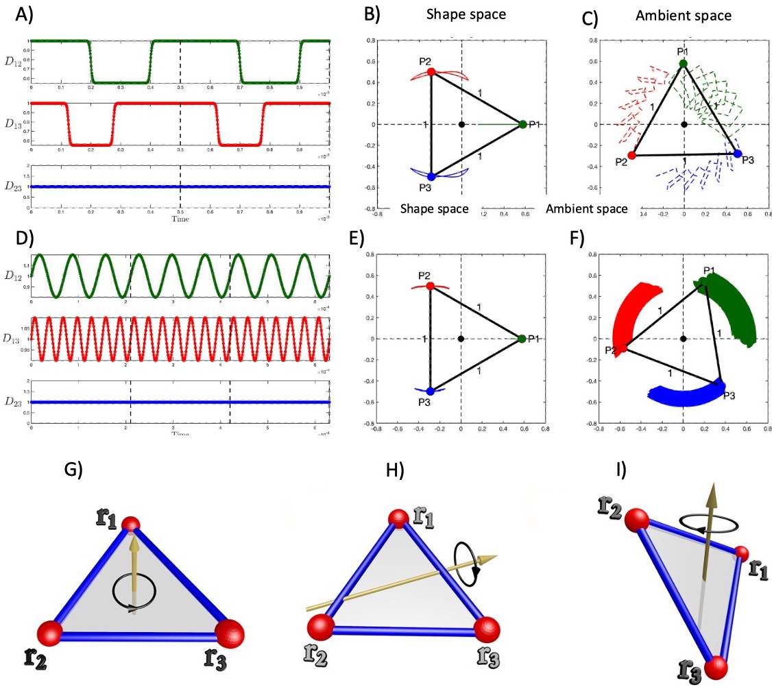
Figure 1: Panel A depicts stepwise changes of bond lengths $D_{12}$ and $D_{13}$ between $D_{1a}=1.0$ and $D_{1a}=0.55$ in an initially equilateral triangle, with $D_{23}=1$ fixed. Panel B shows the motion in shape space, and panel C shows the actual rotational motion. Panels D-F show the same, in case of harmonic bond length oscillations (5) in an initially equilateral triangle $D_{ab}=1$ for $t\in[0,0.1]$ with amplitudes $\Delta D_{12}=0.2$, $\Delta D_{13}=0.1$ and $T_{1}=7\times 10^{-5}$ and $T_{2}=3\times 10^{-5}$. Panel G and H show rotational motions with Hamiltonians (6) and (8) respectively, and panel I depicts a generic rotational motion, as a combination of G and H.

The second example describes the rotational effect of bond length oscillations when $D_{12}$ and $D_{13}$ evolve according to the harmonic oscillator Lagrangian while $D_{23}=1$ is fixed.

$$L=\sum\limits_{a=2,3}\left\{\frac{1}{2}(\frac{dD_{1a}}{dt})^{2}-\frac{1}{2}(\frac{2\pi}{T_{a}})^{2}(D_{1a}-1)^{2}\right\}$$ (5)

At $t=0$ the triangle is equilateral. It then oscillates around its symmetry axis, so that for generic parameter values we observe a net drift as exemplified in panels D-F of Figure 1.

In both examples we observe a qualitative change in the dynamics in the limit of very small amplitudes and very high frequencies. This is the relevant limit for biomolecular applications, where the length and time scales are significantly larger than the individual atom oscillatory amplitudes and periods. The supplementary material’s movie 1 demonstrates how, in both examples, the limit is an equilateral triangle rotating uniformly around its symmetry axis, as in panel G of figure 1. This transition from a triangle with oscillating sites to a uniformly rotating equilateral triangle exemplifies the separation of scales, a general phenomenon that often enables the description of complex systems in terms of a few key variables and commonly introduces qualitatively new features such as self-organization, collective oscillations, and emergent topological order. To describe this limit in our two examples, we take the bond vectors $\mathbf{n}_{i}=\mathbf{r}_{i+1}-\mathbf{r}_{i}$ with $\mathbf{r}_{4}=\mathbf{r}_{1}$ as effective theory dynamical variables, with SO(3) Lie-Poisson brackets Laurent and Hamiltonian

$$H=e\,\mathbf{n}_{1}\cdot\mathbf{n}_{2}\times\mathbf{n}_{3}$$ (6)

Together with the equilateral triangle condition $\mathbf{n}_{1}+\mathbf{n}_{2}+\mathbf{n}_{3}=0$ Hamilton’s equation for $\mathbf{n}_{1}$ is

$$\frac{d\mathbf{n}_{1}}{dt}=\{\mathbf{n}_{1},H\}=-\mathbf{n}_{1}\times\frac{\partial H}{\partial\mathbf{n}_{1}}=\frac{e}{2}(\mathbf{n}_{2}-\mathbf{n}_{3})\ \not=\ 0$$ (7)

with cyclic permutations for $\mathbf{n}_{2}$, $\mathbf{n}_{3}$, and the solution is a uniformly rotating equilateral triangle as in panel G of figure 1. Note that (6) vanishes for a triangle, but the derivatives of $H$ do not vanish. In fact, (7) has no time independent solutions whatsoever, in the case of an equilateral triangle. This qualifies it as an example of a Hamiltonian time crystal Dai-2019 ; Alekseev-2020 , an energy conserving physical system that is in motion even at the minimum of its mechanical free energy Wilczek-2012 ; Shapere-2012 . Apparently cyclopropane C₃H₆ represents this universality class Peng-2021 . The following effective theory Hamiltonian can also be introduced, in the case of a triangle.

$$H=\mathbf{n}_{1}\cdot\mathbf{n}_{2}+g\mathbf{n}_{2}\cdot\mathbf{n}_{3}$$ (8)

For $g\not=1$ it also describes a time crystal, with uniform rotational motion around an axis that lies on the plane of the triangle and goes thru its center with a direction that depends on the parameter $g$, as shown in panel H of figure 1. Finally, panel I depicts a time crystal with a Hamiltonian that is a combination of (6) and (8). With time dependent $e(t)$ and $g(t)$ it can describe any rotational motion of an equilateral triangle around any axis that goes through the center of the triangle.

For tangible molecular examples, we designed polyalanine trefoil knots with varying lengths and studied the impact of their shape deformations using all-atom molecular dynamics simulations in both vacuum and water. We selected polyalanine as it is the simplest side-chained proteinomic amino acid. A closed chain was chosen to limit conformational entropy, making free energy minimization computationally feasible using available computers; notably in the case of an open protein chain the free energy minimization remains a daunting task even for specialized supercomputers Shaw-2021 . The choice of trefoil knot topology for the chain was partially inspired by previous studies Gil-2015 ; horner-2016 ; Segawa-2019 ; vanraden-2019 ; Sawada-2019 that highlighted the potential significance of topology in the functionality of molecular motors. We also anticipate that the chirality of the trefoil knot aids in directing any rotational motion.

For simulations we have utilized GROMACS gromacs with the all-atom CHARMM36m force field charmm36m . We have employed a three-step potential energy minimization protocol that we explain in detail in the Methods section. For our observations, following our triangular examples we have selected a reference triangle defined by three points that are located along the molecule’s backbone, ideally symmetrically and at the positions of C$\alpha$ atoms. We connected these points using virtual segments and used the resulting triangle’s time evolution to characterize the molecule’s rotational motion. For this we used a quaternion representation of rotations Hanson-book :

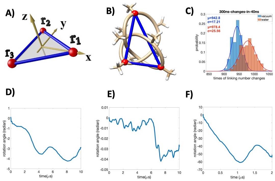
Figure 2: Panel A shows the coordinate system and panel B is the minimum energy 9-ALA, together with the triangle we use to describe its rotational motion. Panel C compares histograms for 9-ALA Gauss linking number changes between -2 and -3 during a 40 $n$s observation period, in vacuum and in water. Panel D shows 9-ALA 2 $\mu$s moving average actual evolution of $\vartheta_{i}$ in (9) in vacuum, panel E shows evolution of $\vartheta_{i}$ in vacuum when evaluated from angular momentum using (10) and panel F shows 0.4 $\mu$s moving average actual evolution of $\vartheta_{i}$ in water.

As shown in panel A of Figure 2, at each time step $t_{i}$ we introduced a cartesian coordinate system, with origin at the center of mass of the entire molecule, and we adjusted the reference triangle so that its geometric center coincided with the molecule’s center of mass. We then assigned to the axes an orthonormal basis of unit quaternions ($\mathbf{\hat{i}}_{i},\mathbf{\hat{j}}_{i},\mathbf{\hat{k}}_{i}$) with $\mathbf{\hat{i}}_{i}$ pointing from the center of mass to one of the vertices of the triangle ($\mathbf{r}_{1}$ in the figure), with $\mathbf{\hat{k}}_{i}$ the normal to the plane of the triangle, and with $\mathbf{\hat{j}}_{i}$ determined by right-handed orthonormality. At time step $t_{i}$ the instantaneous Euler axis of rotation determines a unit quaternion $\mathbf{N}_{i}=x_{i}\mathbf{\hat{i}}_{i}+y_{i}\mathbf{\hat{j}}_{i}+z_{i}\mathbf{\hat{k}}_{i}$ where $x_{i}^{2}+y_{i}^{2}+z_{i}^{2}=1$. The unit normal $\mathbf{k}_{i}$ at time $t_{i}$ is then related to the initial normal vector $\mathbf{k}_{1}$ by

$$\mathbf{k}_{i}=\exp\{-\frac{\vartheta_{i}}{2}\mathbf{N}_{i}\}\,\mathbf{k}_{1}\,\exp\{\frac{\vartheta_{i}}{2}\mathbf{N}_{i}\}$$ (9)

where $\vartheta_{i}$ is the rotation angle around the Euler axis, and we use it to characterize the rotational motion of the triangle relative to the initial triangle: In the case of a rotational motion on a plane $\vartheta_{i}$ coincides with the rotation angle $\theta$ of our triangular examples.

In our simulations the initial molecule had vanishing angular momentum, but due to round-up error accumulation, and Brownian rotational tumbling when water-molecule interactions are present, the angular momentum can fluctuate during the simulation. Thus we monitored its value, to isolate its contribution from the rotational motion of the molecule that is due to shape deformations. For this, imagine that between time steps $t_{i}$ and $t_{i+1}$ the molecule rotates as a rigid body. To describe this ”rigid body” i.e. proper rotation of the molecule, we evaluated the components of the instantaneous moment of inertia tensor $\mathbb{I}_{ab}(i)$ and the components $L_{a}(i)$ of the instantaneous angular momentum. We then evaluated the components of the instantaneous ”rigid body” angular velocity $\omega_{a}(i)=\mathbb{I}^{-1}_{ab}(i)L_{b}(i)$. With $\mathbf{r}_{i}$ is the position of a generic atom with respect to the molecule’s center of mass at time $t_{i}$, its putative ”rigid body” rotated position at $t_{i+1}$ is then

$$\mathbf{r}_{i+1}\ =\ \mathbf{r}_{i}+(t_{i+1}-t_{i})\,\boldsymbol{\omega}_{i}\times\mathbf{r}_{i}$$ (10)

The difference between the actual orientation and the putative orientation evaluated according to (10) is then the rotational motion that we attributed to the molecule’s shape changes; we found that the rotation evaluated using (10) is quite small in comparison to the rotational motion by shape changes. We note that the ”rigid body” rotation (10) is tantamount to a description using instantaneous Eckart frames Eckart-1935 where a rotational motion due to shape changes can not be detected.

Results

We now describe our simulation results for 9 amino acid polyalanine trefoil which is the shortest trefoil knot that we can design without any steric conflicts, and 42-ALA with is the shortest trefoil knot that we can design with all peptide planes in the trans-conformation at energy minimum. In the case of 9-ALA our minimum energy all-atom structure together with the triangle that we used to follow its rotational motion, is shown in Panel B of figure 2. The peptide planes are neither in trans nor in cis conformation implying that the backbone is strained. Notably, the energy minimum breaks spontaneously the three-fold $D_{3}$ trefoil symmetry into a $C_{2}$ symmetry with three distinct, degenerate minimum energy trefoils that are related to each other by $i\to i+3$ $mod(9)$ shift along the backbone. In the case of 42-ALA the $D_{3}$ trefoil symmetry is similarly spontaneously broken into $C_{2}$, with the three energy minima related to each other by a $i\to i+14$ $mod(42)$ shift.

Our vacuum trajectories were 10 $\mu$s long at constant 310 K internal molecular temperature; note that thermal effects could be thought of as rudimental approximation of quantum mechanical zero point fluctuations. In the case of 9-ALA the average C$\alpha$ backbone root-mean-square distance (RMSD) between the initial structure and those along the trajectory was stable at 0.14 $\pm$0.02 Å, and for 42-ALA we obtained RMSD 0.69 $\pm$0.15 Å. The $D_{3}$ symmetries remained broken in both cases. We used Topoly Dabrowski-2021 to evaluate the evolution of Gauss linking number between the C$\alpha$ trace and the virtual C$\beta$ trace, which in the present case is a local topological invariant. For 9-ALA the initial value was -2 and along the trajectory it oscillated frequently between -2 and -3, as shown in panel C of figure 2. For 42-ALA the initial value was -1 and along the trajectory it oscillated between 0 and -2.

Panel D of figure 2 shows the 2 $\mu$s moving average time evolution of the rotation angle $\vartheta_{i}$ in (9), in the case of 9-ALA. Panel A of figure 3 shows the same for 42-ALA. In both, we have back-and-forth oscillations in combination of an overall directed rotational motion, in resemblance of panels C and F in figure 1. The panel E of figure 2 shows the evolution of $\vartheta_{i}$ when evaluated from (10) for 9-ALA, and B of figure 3 shows the same for 42-ALA. Clearly, the contribution from angular momentum fluctuations to the rotational motion due to shape deformations was vanishingly small, in both cases.

We have simulated the 9-ALA trefoil extensively in a solvent with 1157 explicit water molecules at 310 K, and we find that the molecule retains its (average) shape with no indication of $D_{3}$ symmetry restoration: The C$\alpha$ backbone RMSD between the initial structure and those along the trajectory is 0.13 $\pm$0.02 Å. But the water-molecule interactions intensify the frequency of shape fluctuations that drive the molecule’s rotational motion. This can be seen in panel C of figure 2 that shows how the Gauss linking number oscillates between -2 and -3 and a comparison between panels D and F shows how the rotational motion is clearly faster in water. But it becomes difficult to compare the actual rotational motion with the instantaneous rigid body rotation computed from (10). This is because water exchanges angular momentum with the molecule, and in a box with periodic boundary conditions it is problematic to ensure conservation of total angular momentum.

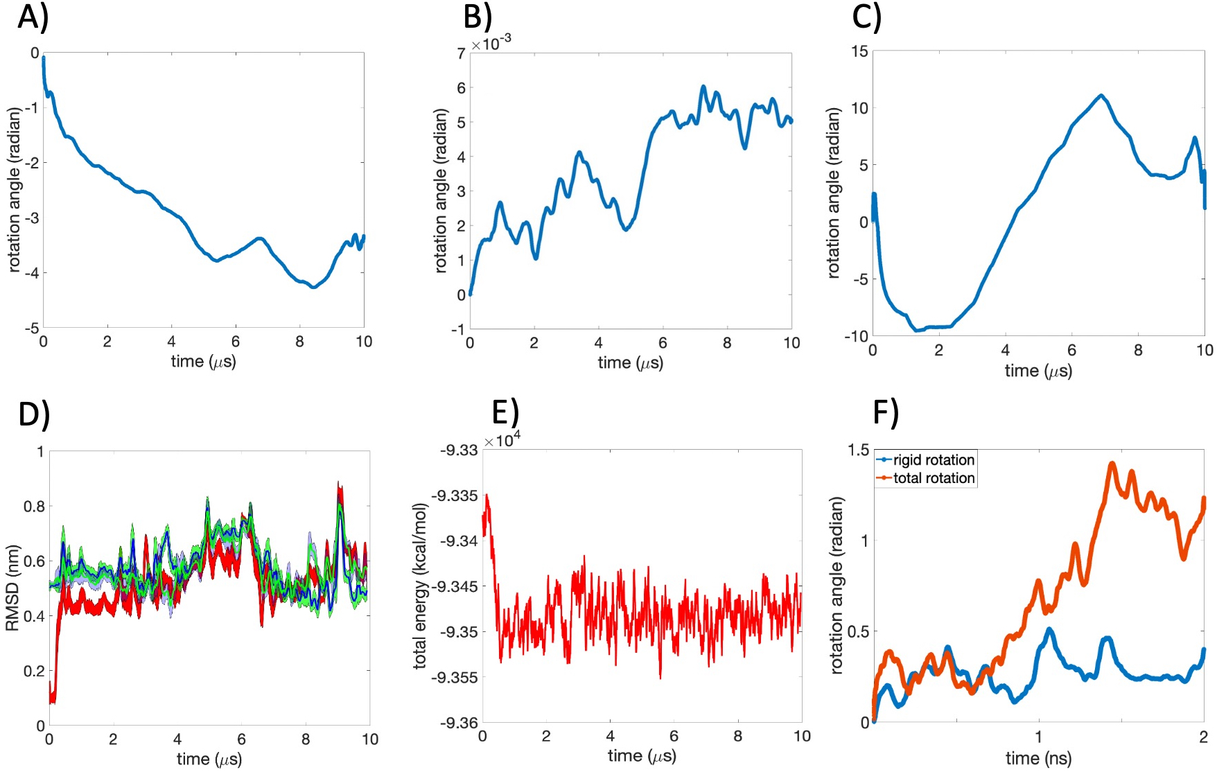
Figure 3: Panel A shows rotational motion of 42-ALA in vacuum in terms of $\vartheta_{i}$ in (9). Panel B shows the $\vartheta_{i}$ evolution in vacuum, when evaluated from instantaneous angular momentum. Panel C shows evolution of $\vartheta_{i}$ in water. Panel D shows RMSD from 42-ALA trajectory in water to initial energy minimum (red), and to the other two $\mathbb{Z}_{3}$ symmetric energy minima (blue and green). Panel E shows total energy along water trajectory of 42-ALA. Panel F shows a generic short segment of the water trajectory, comparing the actual rotational motion to that evaluated from (10). The difference is the rotational motion due to shape deformations.

We have embedded the minimum energy 42-ALA vacuum structure in solvent with 2445 explicit water molecules, and minimized the total energy by gradient descent. The length of our 310 K dynamical production run is 10 $\mu$s. Initially, $\vartheta_{i}$ decreases. But after 200-300 $n$s there is a rapid transition where the direction of rotational motion appears to reverse (panel C of figure-3), the RMSD between the initial structure and those along the trajectory increases to $\sim$4.5 Å, the RMSD from the trajectory to the two other $C_{2}$ symmetric energy minima approach the same value (panel D), and the Gauss linking number of the C$\alpha$-C$\beta$ traces changes from -1 $\pm 1$ to -9 $\pm$2. The total energy also decreases, as shown in panel E: We conclude that the spontaneously broken $D_{3}$ symmetry becomes restored, in a manner that resembles a second order phase transition akin the ferromagnetic to paramagnetic phase transition in magnetic materials. Panel F in figure 3 compares the observed rotational motion to that computed from (10). There is a clear distinction between the two.

In the limit of large stroboscopic time steps where an effective theory description becomes valid, the dynamics both in the case of 9-ALA and 42-ALA resembles a tumbling time crystal with the evolution of the reference triangle described by a Hamiltonian that is a sum of (6) and (8) with time dependent parameters $e(t)$ and $g(t)$

Conclusions

Our high-precision all-atom molecular dynamics study shows that the concept of a connection can be essential to the design and control of effective molecular machines. Our results demonstrate how biomolecules can convert individual atom thermal vibrations into a rotational motion of the entire molecule by utilizing the connection in their shape space. This challenges the prevailing view of molecular motors as rigid bodies by highlighting the crucial role of deformability in their functionality. In particular, we have discovered that the impressive effectiveness of many biomolecular motors can be modeled by an effective theory Hamiltonian time crystal while at the atomic level the dynamics is driven by the heat bath of ambient water molecules. We have also exposed the dynamical consequences of a spontaneous symmetry breakdown and restoration. Finally, although simulations of open protein chains are computationally much more demanding we expect our findings to hold true for such systems as well.

Additional information

Data and code availability: Raw data and analysis codes are available from the corresponding author.

Supplementary material:

The supplementary material consists of two movies, and description of simulation methods

$\bullet~{}$ The first movie in file movie1.mp4 describes the qualitative change in dynamics in the case of the model Lagrangian defined in equation (5) in the text. The movie starts with parameter values that describe an oscillating triangle, with no observable rotational motion. Then the parameters including time scale change stepwise. As a consequence the frequency of oscillations increase and their amplitudes decrease and eventually become vanishingly small. At the same time the rotational motion becomes more apparent, until the triangle appears to rotate uniformly in line with the scaling limit effective theory timecrystalline Hamiltonian (6), even though the angular momentum vanishes.

$\bullet~{}$ The second movie in file movie2.mp4 displays a segment of the trajectory of the 42-ALA in water at 310 K, as described in the text. It shows the first 1.0 $\mu$s with 10 $n$s between frames, starting from the initial condition and covering the $C_{2}\to D_{3}$ symmetry restoring transition. The rotational motion is clear from the orientation of the reference triangle, and the structural change during the symmetry restoration can be seen by comparing the first and last frames.

Simulation Methods

In our all-atom polyalanine trefoil knot simulations we use GROMACS gromacs with the all-atom CHARMM36m force field charmm36m . We first minimize the free energy, using a three-step protocol. For this we start with vacuum, with free boundary conditions and both Coulomb and van der Waals interactions extending over all atom pairs in the molecule with no cut-off approximation.

$\bullet$ In step one we start with the trefoil template

$$\begin{split}&x(s)=(2+\cos 3s)\cos 2s\\ &y(s)=(2+\cos 3s)\sin 2s\ \ \ \ \ \ \ \ \ s\in[0,2\pi]\\ &z(s)=\sin 3s\end{split}$$

We discretize this into a linear polygonal chain with $n$ equidistant vertices; $n=9$ and 42 in othe examples we describe in the text. The neighboring vertices are 3.8 Å apart, which is the average distance between neighboring C$\alpha$ atoms along a protein backbone. We use PULCHRA Rotkiewicz-2008 to construct an initial all-atom representation.

$\bullet$ Step two minimizes the energy using a kinetic diffusion process. This consists of an iterative series of energy conserving double precision all-atom runs. For each run we choose the initial kinetic energies of all the atoms to be zero. The typical length of a single run is 1.0 $p$s, during which some of the excess potential energy becomes converted into kinetic energy of the atoms, that we remove to start the next iteration. We repeat the process until we observe no kinetic energy, and minimize the final potential energy using LBFG Byrd-1995 .

$\bullet$ Step three aims to remove the above structure from a putative local energy minimum towards a global minimum, using double precision annealing. We start with a 10 $n$s heating phase from 0 K to 500 K followed by a 5 $n$s stabilization. We then proceed to a 985 $n$s cooling simulation that brings the temperature back to 0 K.

We repeat the steps two and three until we observe no energy decrease in the final 0 K configuration. This proposes that we have reached the minimum of the molecule’s potential energy. In the case of 9-ALA our minimization algorithm decreases the CHARMM36m energy from the initial value 25583 kJ/mol down to 6120 kJ/mol and in the case of 42-ALA the CHARMM36m energy goes down from 6255 kJ/mol to 1764 kJ/mol.

We then employ energy drift, a common phenomenon in all-atom simulations, to construct the corresponding finite temperature minimum energy configuration: We initiate a single precision run with 1.0 $f$s time step. Due to error accumulation the internal temperature of the molecule starts increasing, and we let the energy drift proceed until the temperature has reached a target value, 310 K in the examples that we present here. This gives us the initial configuration of our production runs in vacuum.

A tight knotted protein such as our polyalanine trefoils, is subject to steric restraints proposing that the minimum energy configurations in vacuum and in water should be geometrically close to each other. Thus, we start all our water simulations by placing the above 310 K minimum energy molecule at the center of a cubic box with periodic boundary condition, with 12 Å  distance to the edges. We fill the box with explicit TIP3P TIP3P water, with 12 Å  cutoff for Coulomb and van der Waals interactions. We then minimize the potential energy of the entire system, using gradient descent to construct a minimum energy ensemble. We bring the entire system in thermal equilibrium at 310 K, and we start the production run always with vanishing initial angular momentum. We keep the simulation time step short enough to eliminate detectable energy drift, and we use double precision as need be.