Fully-Passive Twin-Field Quantum Key Distribution

Abstract

We propose a fully-passive twin-field quantum key distribution (QKD) setup where basis choice, decoy-state preparation and encoding are all implemented entirely by post-processing without any active modulation. Our protocol can remove the potential side-channels from both source modulators and detectors, and additionally retain the high key rate advantage offered by twin-field QKD, thus offering great implementation security and good performance. Importantly, we also propose a post-processing strategy that uses mismatched phase slices and minimizes the effect of sifting. We show with numerical simulation that the new protocol can still beat the repeaterless bound and provide satisfactory key rate.

Background. For a practical quantum key distribution (QKD) system, active modulation devices in a source might introduce additional side-channels [1, 2] or be susceptible to Trojan horse attacks [3, 4], leaking information to Eve. Therefore, it would be ideal if we can remove the modulation devices in the source and implement decoy-state setting choice [5, 6, 7] and the encoding of signals passively by post-selection or post-processing only.

Passive decoy-state [8, 9] and passive encoding [10] schemes have both been proposed for BB84 systems. More recently, fully passive BB84 schemes [11, 12] combining both passive decoy-state preparation and encoding have also been proposed, which entirely remove active modulators in the source. Passive state-preparation has also been implemented for Gaussian-modulated continuous-variable (CV) QKD [13] and very recently for discrete-modulated CV-QKD [14].

All the above passive schemes, however, aim at removing side-channels in source modulators. We can further improve the implementation security of the system if we can apply passive encoding and decoy-state choice to measurement-device-independent (MDI) protocols [15, 16], which can remove side-channels in detectors. Particularly, the new twin-field (TF) QKD [16] protocol can provide both measurement-device-independence and exceptionally high key rate. In fact it can beat the upper bound for the rate-distance trade-off relation without a repeater [17] and so far has enabled QKD over as far as 1000 kilometers [18]. Ever since its proposal, TF-QKD has led to much theoretical interest [19, 20, 21, 22, 23, 24, 27, 26, 25] in recent years and many experimental demonstrations [28, 29, 30, 31, 32, 34, 35, 36, 37, 33]. While there has been a recent proposal for passive decoy-state TF-QKD [38], it still requires active modulators for encoding. So far, there has never been any passive-encoding (or fully-passive) scheme for TF-QKD.

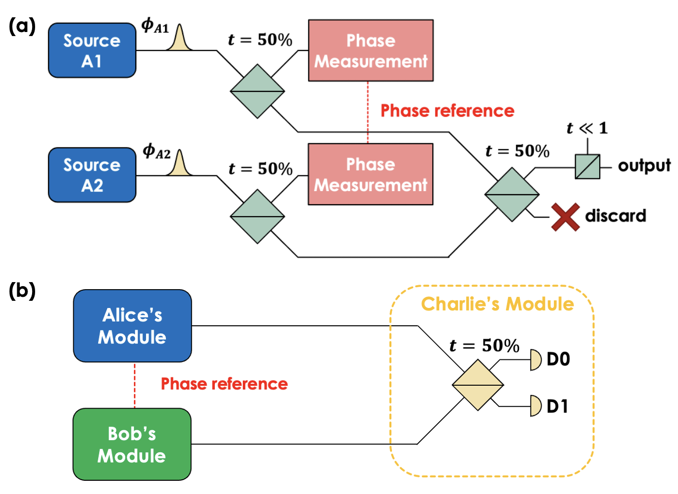
Figure 1: (a) The setup for a single source module for Alice (Bob holds an identical module with sources B1 and B2). Alice prepares two strong laser pulses and splits off each of them respectively to measure the phases $\phi_{A1}$ and $\phi_{A2}$. She then let the two pulses interfere, and attenuates one of the output port to single-photon level before sending off the output signal to Charlie. Alice can also replace the “discard” port with a classical detector, but the detection results are already implied by $\phi_{A1}$ and $\phi_{A2}$. (b) The overall setup for fully passive TF-QKD where Alice and Bob prepare signals and send them to a third untrusted party Charlie, who performs a swap test and publicly announces the results. Alice and Bob also need a common phase reference, e.g. sent by Charlie, or established by Alice and Bob sending strong pulses to Charlie for comparison and feedback.

In this work, we build upon the CAL TF-QKD protocol [23] and propose the first fully passive TF-QKD scheme, where all the encoding, decoy-state setting choice, as well as even the basis choice, are entirely generated by post-processing, and all the degrees-of-freedom (DOFs) come from the randomness of the phases from the laser sources themselves. To address the main challenge of heavy sifting (which would occur if one performs naive post-selection), we also propose a set of post-processing strategies that match phase slices and maximize the amount of signals used, reducing loss in key rate due to sifting. This allows us to have a protocol with very high implementation security with no side-channels in either detectors or source modulators [39] as well as satisfactory key rate.

Setup. In the passive setup, we make use of two independent laser sources for each of Alice and Bob, which we denote as sources A1,A2,B1 and B2. The pulses are first generated at strong intensity levels, which allow us to split off the pulses and measure classically the phases of all pulses (e.g. by interfering with a reference laser), which we can denote as $\phi_{A1},\phi_{A2},\phi_{B1}$ and $\phi_{B2}$. For simplicity, we set the four laser sources to all output pulses at the same intensity $\mu_{max}/2$.

The most crucial assumption here is that the phases are all independent and random, i.e. uniformly distributed between $[0,2\pi)$. Such inherent phase randomness in laser sources have already been used for QKD systems and quantum random number generators (QRNGs) [40, 41, 42, 43, 44]. We also assume that Alice and Bob can establish a common phase reference for all their measurements.

Alice (Bob) first lets A1 and A2 (B1 and B2) interfere, and the signal from one output port is then attenuated to single-photon level, and sent to the relay Charlie, who lets the incoming two beams interfere and announces the click events from detectors D0 and D1. Alice (Bob) can optionally observe the other output port of their local interferometer to obtain the output intensity, but this information is also already contained in $|\phi_{A1}-\phi_{A2}|$ ($|\phi_{B1}-\phi_{B2}|$). The setup can be seen in Fig. 1.

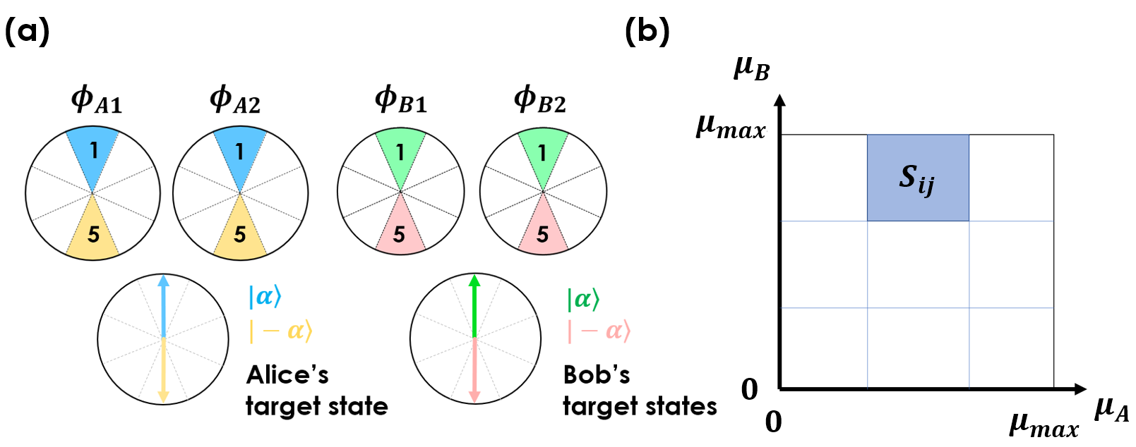
Figure 2: (a) The post-selection of phase-slices for Alice and Bob in the coding phase (X basis). Alice and Bob each only post-select cases where their local two phases are in the same slice and the slice happens to have an index of $k=1$ or $k=N/2+1$ corresponding to $0$ and $\pi$ phases (here total slice number is $N=8$). Note that Alice and Bob can further use mismatched slices to generate key (details are described in Appendix C). (b) The post-selection of decoy intensities for Alice and Bob. They can e.g. divide the domain into a $3\times 3$ grid where each $S_{ij}$ corresponds to a decoy setting.

Protocol. We can use the above setup to implement fully passive CAL TFQKD [23].

1. Alice and Bob simply prepare the states based on the setup in Fig. 1 and send out the signals without any modulation, while recording the locally measured $\phi_{A1},\phi_{A2},\phi_{B1}$ and $\phi_{B2}$. Charlie announces the detection results $k_{c},k_{d}$ from detectors $D_{0}$ and $D_{1}$.

2. During post-processing, Alice and Bob first each randomly chooses between a coding phase (X basis) and a decoy phase (Z) based on local random classical bits. They announce their basis choice.

   (1) In the signal X basis, Alice and Bob divide up the $[0,2\pi)$ domain of phases into N slices (N is an even number), and assign each of the phases they measured into a slice, indexed by $k$ (we can denote the indices respectively by $k_{A1},k_{A2},k_{B1}$ and $k_{B2}$). In the simplest form of post-selection, Alice (Bob) only announces a successful event if the two local phases $\phi_{A1}$ and $\phi_{A2}$ ($\phi_{B1}$ and $\phi_{B2}$) fall within the same slice, and the slice happens to have an index of $k=1$ or $k=N/2+1$ (i.e. target states are $\phi=0$ or $\phi=\pi$) and discard the event otherwise, as shown in Fig. 2 (a). Alice and Bob keep their slice indices secret (which correspond to their classical bits $0$ or $1$).

   (2) In the decoy Z basis, Alice and Bob each post-selects their signals based on $|\phi_{A1}-\phi_{A2}|$ and $|\phi_{B1}-\phi_{B2}|$, which is equivalent to measuring and post-selecting the output intensities $\mu_{A}$ and $\mu_{B}$, both of which randomly lie between $[0,\mu_{max}]$ following an intensity probability distribution $p(\mu)=1/(\pi\sqrt{\mu(\mu_{max}-\mu)})$ [11]. Alice and Bob can simply divide the ranges into continuous post-selection regions $S_{ij}$ (similar to passive decoy-state method [8]) and announce the region the signal each falls in. For instance, they can simply divide the domain equally into $3\times 3$ square regions, which conceptually correspond to the intensity set of $\{\mu,\nu,\omega\}\times\{\mu,\nu,\omega\}$ for active TF-QKD. They can then perform decoy-state analysis and estimate photon-number yields $Y_{mn}$.

3. Alice and Bob perform sifting of basis, perform error-correction on their raw key obtained from the coding phase, and perform privacy amplification, the amount of which is estimated using the upper-bounded phase error rate and also the classical information leakage (in the same fashion as active TF-QKD).

While the above protocol is already a functioning fully-passive CAL TF-QKD scheme, the main drawback of it would be the heavy sifting due to post-selection (there is only a low probability that scales with $1/N^{4}$ for Alice and Bob’s slices to follow the pattern in Fig. 2). To address this problem, we propose a post-processing strategy where Alice and Bob can match up the originally-discarded slices that do not have the same index to improve sifting. Any combination of $\{k_{A1},k_{A2},k_{B1},k_{B2}\}$ can be potentially used to generate key. Some highly mismatched combinations might have zero key rate, but they will have no detrimental effect to the total key rate since we can choose only the combinations with positive key rate to generate key.

In the improved sifting scheme, Alice and Bob do not have to choose slices corresponding to $0$ and $\pi$ phases, but instead, any pair of $\phi_{G}$ and $\phi_{G}+\pi$ can be used to generate key (since Charlie only measures the phase difference between incoming pulses), i.e. Alice and Bob can use any pair of $k=l$ or $k=N/2+l$ and publicly announce their reference point index $l$ (so long as they each still choose between states with $0$ or $\pi$ phase differences with respect to the reference point $\phi_{G}$ and keep this choice secret). Additionally, it is possible to have mismatched local slices ($k_{A1}\neq k_{A2}$ and $k_{B1}\neq k_{B2}$, which correspond to smaller and potentially unequal signal intensities for Alice and Bob) and mismatched phase references between Alice and Bob ($k_{A1}\neq k_{B1}$, which corresponds to a misalignment between Alice and Bob). More details on this strategy can be found in Appendix C. The final key rate can simply be a summation of the key rates from all combinations for Alice’s and Bob’s slices.

$$R= {1\over{N^{4}}}\sum_{k_{A1}=1}^{N}\sum_{k_{A2}=1}^{N}\sum_{k_{B1}=1}^{N}\sum_{k_{B2}=1}^{N}$$ (1)

$$[\max(0,R_{0,1}(k_{A1},k_{A2},k_{B1},k_{B2}))$$

$$+\max(0,R_{1,0}(k_{A1},k_{A2},k_{B1},k_{B2}))],$$

which includes a sifting factor of $1/N^{4}$ corresponding to the probability of signals falling within each pattern of slices [45]. The subscripts of $R_{k_{c},k_{d}}$ corresponds to detection patterns from Charlie.

Importantly, since we add up all combinations of phase slices, increasing the slice number $N$ does not affect the sifting factor and only increases the key rate. Our slice size is only limited by the accuracy and resolution of the classical local detection (at least in the asymptotic scenario with infinite data size, which is the focus of this work. Finite-size analysis will be the subject of future studies.). This is the main reason why, as we will later show, our key rate is only moderately lower than the active counterpart, despite we are slicing and matching the phases for four independent sources.

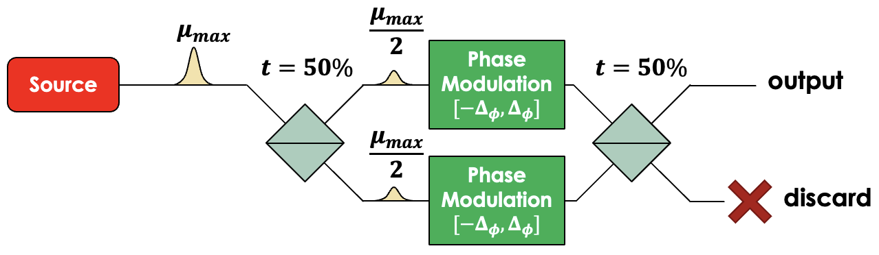
Figure 3: (a) An equivalent local quantum channel $\mathcal{E}_{A}$ inside Alice’s lab, which perturbs an otherwise perfect laser source with intensity $\mu_{max}$ into the physical output signal from the setup in Fig. 1 (a). The same channel can be assumed inside Bob’s lab.

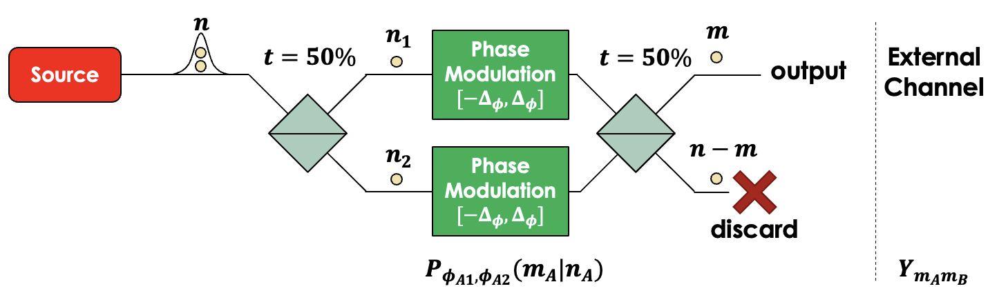
Figure 4: After we apply the Cauchy-Schwartz inequality and convert the source into a summation of $n_{A}$ photon number states, the local channel $\mathcal{E}_{A}$ is equivalent to a local lossy channel for an $n_{A}$ photon state and potentially reduces it to $m_{A}$ photons with probability of $P_{\phi_{A1},\phi_{A2}}(m_{A}|n_{A})$. A similar process applies to Bob. The local transmittances at Alice and Bob are multiplied to the external channel yield $Y_{m_{A}m_{B}}$, which can be estimated from the decoy-state analysis.

Security. In the fully passive CAL TF-QKD scheme, the main difference from the active counterpart would be the finite size of the phase slices, $\Delta_{\phi}=\pi/N$ (for convenience, we define a slice to be $2\Delta_{\phi}$). This can be considered as a type of source preparation imperfection: (1) the signal state QBER would be inherently higher due to the slightly mismatched phases of Alice and Bob’s signals, even if they choose the same slice, e.g. $k=1$; (2) the characterization of the source states (which were just $\ket{\alpha},\ket{-\alpha}$ for active TF-QKD) is imperfect, since the interference of e.g. sources A1 and A2 with finite phase slices results in fluctuations in both the source intensity and the source encoding (phase). This may result in a security loophole and need more careful discussions.

Here we consider a local quantum channel [46, 47, 48] $\mathcal{E}_{A}$ ($\mathcal{E}_{B}$) inside Alice’s (Bob’s) lab, as shown in 3. The channel accepts a perfectly prepared source with intensity $\mu_{max}$. The signal is split evenly in two and a random phase modulation between $[-\Delta_{\phi},\Delta_{\phi}]$ is applied on each path. The signals are re-combined to interfere at a second beam splitter, one output of which is directed to the output and the other port is discarded. A perfect source going through this quantum channel will generate the exact same statistics as that of the physical source in Fig. 1 (a) after Alice post-selects slices $k_{A1}=1$ and $k_{A2}=1$ [49].

Therefore, we can pessimistically “yield” this quantum channel to Eve and consider it as part of the external channel under Eve’s control. In the signal X basis, this simply means that the higher QBER (physically due to finite phase slices) can be considered part of the channel and it only increases error-correction cost.

For the conjugate Z basis, we recall that in CAL TF-QKD [23], we establish a virtual protocol with cat states in Z basis, and apply the Cauchy-Schwartz inequality to bound their statistics (the phase error rate) with yields from photon number states, $Y_{m_{A}m_{B}}$ we estimate from real WCP states as decoy-states. Here for passive TF-QKD, the yields we obtain from decoy-state analysis only represent the external physical channel and do not include the effect of $\mathcal{E}_{A}$ and $\mathcal{E}_{B}$. We observe that the local channels can in fact be represented as just local losses, as shown in Fig. 4, which reduce e.g. $n_{A}$ photons to $m_{A}$ photons with probability $P_{\phi_{A1},\phi_{A2}}(m_{A}|n_{A})$. The actual yield can be written as:

$$Y_{n_{A}n_{B}}=\int_{-\Delta_{\phi}}^{\Delta_{\phi}}\int_{-\Delta_{\phi}}^{\Delta_{\phi}}\int_{-\Delta_{\phi}}^{\Delta_{\phi}}\int_{-\Delta_{\phi}}^{\Delta_{\phi}}$$ (2)

$$\sum_{m_{A}=0}^{n_{A}}\sum_{m_{B}=0}^{n_{B}}P_{\phi_{A1},\phi_{A2}}(m_{A}|n_{A})P_{\phi_{B1},\phi_{B2}}(m_{B}|n_{B})Y_{m_{A}m_{B}}$$

$$d\phi_{A1}d\phi_{A2}d\phi_{B1}d\phi_{B2},$$

which can be used to calculate the corrected phase error rate. The detailed expressions and derivation can be found in Appendix D.

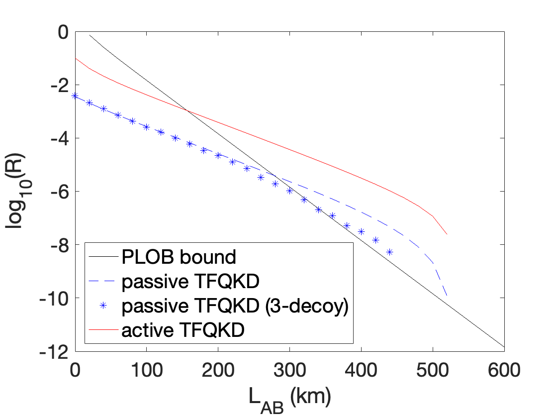
Figure 5: Simulation of the key rate for passive TF-QKD versus active TF-QKD. Here we only consider the scenario of infinite data size. The PLOB bound [17] is also included for comparison. We generate key rate for passive TF-QKD for both the asymptotic case with infinite decoys and the case with three decoy settings for each of Alice and Bob. As can be seen, passive TF-QKD only has moderately lower key rate than the active counterpart and is still able to surpass the PLOB bound under practical settings.

Results. Here we perform a simple simulation for passive TF-QKD versus its active counterpart in the asymptotic limit of infinite data size and infinite decoys (i.e. we assume Alice and Bob can estimate $Y_{m_{A}m_{B}}$ perfectly). We set a dark count rate of $p_{d}=10^{-8}$, no misalignment, a fiber loss of $0.2dB/km$, detector efficiency of $\eta_{d}=1$ (the efficiency can be equivalently incorporated into channel loss) and an error correction efficiency of $f_{e}=1$. Here for simplicity, the signal intensity is first optimized for active TF-QKD and also used for the passive protocol (ranging from approximately $\mu_{max}=0.01$ to $0.12$ depending on distance) [50] and we fix the slice number to a reasonably large value $N=24$.

We also plot the key rate with three passive decoy settings for each of Alice and Bob (using the $3\times 3$ grid decoy regions as shown in Fig. 2 (b)), where we choose regions of $[0,0.3\mu_{max})$, $[0.3\mu_{max},0.7\mu_{max})$, and $[0.7\mu_{max},\mu_{max}]$. More details on the active and passive decoy analysis models used in the simulation are included in Appendix F.

The results are shown in Fig. 5. As can be seen, the passive TF-QKD scheme still yields satisfactory key rate and can exceed the linear repeaterless bound [17]. The asymptotic key rate is about 1.2 orders-of-magnitude lower than the active counterpart, due to the inherent QBER and increased local losses resulting from finite phase slices, in exchange for the much better implementation security. The key rate using three decoy settings is lower than that of the infinite-decoy case at longer distances, mainly due to decoy intensities being relatively small (since all decoy intensities are no larger than $\mu_{max}$), although it can still beat the PLOB bound.

Note that, however, the main purpose of the passive TF-QKD scheme is not to reach a record-breaking key rate, but rather to provide a higher implementation security than either active BB84 or active TF-QKD (while still maintaining good key rate), and it would be useful not only at long distances, but even at close-to-medium distances (where it does not beat the PLOB bound), such as in a metropolitan network with untrusted relays and multiple users.

Discussions. In this work, we have proposed a passive TF-QKD protocol that removes both detector and source modulator side-channels while also offering satisfactory key rate.

A main challenge for implementing the scheme experimentally would be maintaining (1) a common phase reference between the distant parties Alice and Bob, as well as (2) a good interference visibility between all four laser sources (including timing and frequency stability). Stability of interference between the local pairs of sources can be addressed by using a time-delay scheme [11] that allows each of Alice and Bob to just use a single laser. The bigger challenge, on the other hand, is to remotely establish the global phase reference and maintain the frequency stability between Alice and Bob. This is also a challenge for active TF-QKD schemes, which usually use phase-locking schemes that send reference signals (from Charlie or locally from Alice) through service fibers to Alice and Bob respectively, implementing optical phase locked loops [30, 31, 34, 36, 37], time-frequency metrology [29, 37], or injection locking [32, 35] (citing categorization from Ref. [52] Table I). However, a unique challenge passive TF-QKD faces is that we need independent phase randomness between Alice’s and Bob’s sources, making phase-locking no longer viable. In principle, though, Alice and Bob can send strong signals to Charlie and evaluate their phase drift, and use classical feedback mechanisms (e.g. temperature control at source, or post-processing/compensation at Charlie) to maintain the frequency stability between signals [51]. For instance, there have very recently been proposals for TF-QKD schemes that achieve frequency stability without phase-locking using compensation at Charlie’s station only [52, 53]. An experimental demonstration of the fully passive TF-QKD scheme as well as a finite-size analysis for the passive TF-QKD protocol would be subjects of future work.

Appendix A Comparison with Fully Passive BB84

We have recently proposed a fully-passive BB84 scheme [11], which can impressively also remove active modulators for both decoy-state choice and encoding. The scheme can also potentially be used for fully passive measurement-device-independent QKD.

However, Ref. [11] focuses on a polarization encoding setup (or an equivalent time-bin phase encoding scheme) involving two different optical modes, and post-selects from states spanning the entire 3D Bloch sphere. This is a very different idea from what we propose in this work for TF-QKD, which always prepares states in the same polarization mode and performs slicing and matching for just the different relative phases between pulses.

Additionally, fully passive TF-QKD can eliminate side-channels from not only source detectors, but also detectors, enabling higher implementation security than either fully-passive BB84 or active QKD. While future applications of the fully passive source in Ref. [11] to MDI-QKD can potentially offer similar protection against detector side-channels, a fully passive TF-QKD scheme can potentially provide better scaling of key rate versus distance.

Appendix B The CAL Twin-Field QKD Protocol

Here we present a brief recapitulation of the CAL TF-QKD protocol [23], which the passive protocol in this work is based on.

In the encoding basis X, Alice and Bob encode information by sending the states (for simplicity here we only show Alice’s system, and Bob’s system has the identical form but with suffixes $B$ and $b$):

$$\ket{+}_{A}\ket{\alpha}_{a}+\ket{-}_{A}\ket{-\alpha}_{a}$$ (3)

in the X basis.

In a virtual protocol, Alice sends cat states in the Z basis:

$$\ket{0}_{A}(\ket{\alpha}_{a}+\ket{-\alpha}_{a})/\sqrt{2}+\ket{1}_{A}(\ket{\alpha}_{a}-\ket{-\alpha}_{a})/\sqrt{2}$$ (4)

$$= \ket{0}_{A}\ket{C_{0}}_{a}+\ket{1}_{A}\ket{C_{1}}_{a},$$

where $\ket{C_{0}}_{a}$ and $\ket{C_{1}}_{a}$ are (unnormalized) cat states.

Alice and Bob measure their local qubits in X or Z bases. The phase error rate for the signal states is simply the bit error rate for the cat states. Moreover, using Cauchy-Schwartz inequality, any statistics for the cat states (which are superpositions of photon number states) can be upper-bounded by statistics of a mixture of photon number states. The upper bound for the phase error can be written as [23]:

$$Q_{k_{c},k_{d}}^{X}e_{k_{c},k_{d}}^{Z}$$ (5)

$$\leq\sum_{j=0,1}\left[\sum_{n_{A},n_{B}=0}^{\infty}c_{m_{A}}^{A,(j)}c_{m_{B}}^{B,(j)}\sqrt{Y^{Z}_{{k_{c}},{k_{d}},m_{A}m_{B}}}\right]^{2},$$

where $Y^{Z}_{{k_{c}},{k_{d}},m_{A}m_{B}}$ is the yield for the $n_{A},n_{B}$ photon number state (here instead of using the notation $Y_{m_{A}m_{B}}$, in the following Appendices we use the more detailed notation from Ref. [23] and include the basis $Z$ and detection event $k_{c},k_{d}$ information), and the coefficients for cat states are:

$$c_{n_{A}}^{A,(j)} =[(e^{-|\alpha_{A}|^{2}/2}{{\alpha_{A}^{n_{A}}}\over{\sqrt{n_{A}!}}})$$ (6)

$$+(-1)^{j}\times(e^{-|\alpha_{A}|^{2}/2}{{(-\alpha_{A})^{n_{A}}}\over{\sqrt{n_{A}!}}})]/2,$$

$$c_{n_{B}}^{B,(j)} =[(e^{-|\alpha_{B}|^{2}/2}{{\alpha_{B}^{n_{B}}}\over{\sqrt{n_{B}!}}})$$

$$+(-1)^{j}\times(e^{-|\alpha_{B}|^{2}/2}{{(-\alpha_{B})^{n_{B}}}\over{\sqrt{n_{B}!}}})]/2.$$

In practice, instead of using real cat states, in the Z testing basis, Alice and Bob prepare phase-randomized WCP states in various intensity settings, which can be used to construct a linear program and solve for $n_{A},n_{B}$-photon yields $Y^{Z}_{{k_{c}},{k_{d}},n_{A}n_{B}}$ that is used above to calculate the phase error rate.

The secure key rate is

$$R_{k_{c},k_{d}} =Q^{X}_{k_{c},k_{d}}[1-h_{2}(e^{Z}_{k_{c},k_{d}})-f_{e}h_{2}(E^{X}_{k_{c},k_{d}})],$$ (7)

where $f_{e}$ is the error-correction efficiency and $E^{X}_{k_{c},k_{d}}$ the observed quantum bit error rate in signal basis. The final key rate sums up the two detection patterns

$$R =R_{0,1}+R_{1,0}.$$ (8)

Appendix C Phase Slice Matching Strategy

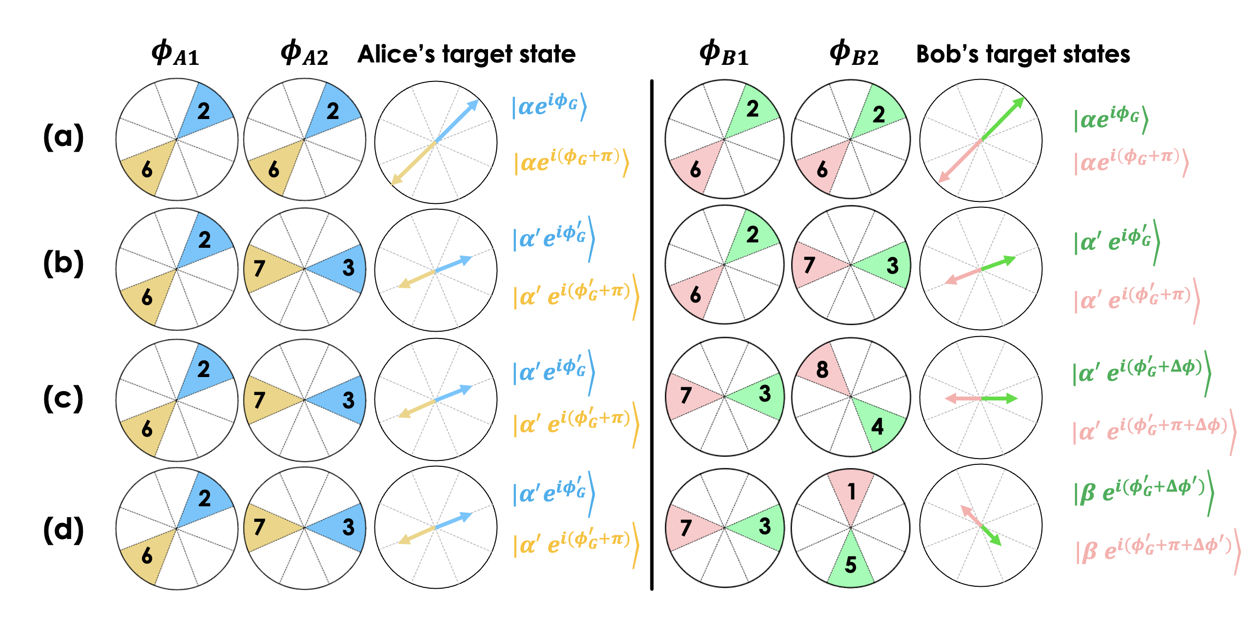
Figure 6: Types of mismatch between phase slices for sources A1, A2, B1, and B2. We also show the target states (the asymptotic limit of the state if the slice size is infinitely small) to be prepared. All types of mismatch only affect the key rate and will not require additionally modified security analysis. (a) Alice and Bob’s phase reference points are not $k=1$ (i.e. not $\phi=0$); (b) Alice and Bob’s local slices are not the same; (c) Alice and Bob’s phase reference points are different; (d) The amount of mismatch between Alice and Bob’s local slices are different. The above types of mismatch give us four degrees-of-freedom and can be used to describe any combination of $\{k_{A1},k_{A2},k_{B1},k_{B2}\}$.

Here we describe in more detail the phase slice matching strategy that we propose in order to minimize the amount of discarded signals.

As mentioned in the main text, we allow Alice and Bob to generate key with any combination of phase slices for sources A1, A2, B1, and B2, indexed by $k_{A1},k_{A2},k_{B1}$ and $k_{B2}$. Compared to the default case as shown in Fig. 2 where Alice and Bob both pick the same local slice and both use the same phase reference, there are four possible types of mismatches, which we show in Fig. 6. We will proceed to explain that all of these mismatches are already included in the current framework and do not need additional revision to the security analysis:

1. As shown in Fig. 6 (a), the global phase reference for Alice (and also Bob) is not zero. This does not have any effect on either bit error rate (since it generates identical statistics at Charlie, who only compares phase difference between Alice and Bob) or the phase error rate (since the effect is equivalent to a phase drift in the external channel and does not yield any additional information to Eve), leading to the same secure key rate as slices with phase reference point at zero.

2. As shown in Fig. 6 (b), the local slices are mismatched at Alice (and also Bob). This results in a shifted phase reference (which has no effect on the key rate so long as the amount of shifting is the same for Alice and Bob) and also a smaller average signal intensity. A smaller average intensity simply changes the coefficients for the cat state and does not affect security, while the fluctuation of intensity and phase will be addressed in the next section in the security analysis.

3. As shown in Fig. 6 (c), Alice and Bob’s phase references can be different. This is equivalent to a channel misalignment and will result in higher QBER and lower key rate, but will not affect the security.

4. As shown in Fig. 6 (d), the amount of mismatch between Alice’s and Bob’s local slices can be different. This on the one hand results in a different phase reference (same as mentioned above), and also results in asymmetry between Alice’s and Bob’s average signal intensities. As discussed in Ref. [26], the cat states for Alice and Bob are independent and are allowed to have different coefficients. Asymmetric signal intensities simply result in worse visibility (hence higher QBER) when channels are symmetric, but might be beneficial if the physical channels are asymmetric to begin with.

These four degrees-of-freedom $x_{1}=(k_{A1}+k_{A2})/2$, $x_{2}=k_{A2}-k_{A1}$, $x_{3}=(k_{A1}+k_{A2})/2-(k_{B1}+k_{B2})/2$, and $x_{4}=(k_{B2}-k_{B1})-(k_{A2}-k_{A1})$, are sufficient to represent all combinations of $\{k_{A1},k_{A2},k_{B1},k_{B2}\}$, meaning that the use of any such combination will be a legitimate setup for CAL TF-QKD (and will allow the same form of the bounds on the key rate, without introducing any security loophole). Therefore, we can simply add up the non-zero key rates, in the form of Eq. 1.

Additionally, for the sole purpose of simplifying the calculations, we can calculate:

$$R= {1\over{N^{3}}}\sum_{k_{A2}^{\prime}=1}^{N}\sum_{k_{B1}^{\prime}=1}^{N}\sum_{k_{B2}^{\prime}=1}^{N}$$ (9)

$$[\max(0,R_{0,1}(0,k_{A2}^{\prime},k_{B1}^{\prime},k_{B2}^{\prime}))$$

$$+\max(0,R_{1,0}(0,k_{A2}^{\prime},k_{B1}^{\prime},k_{B2}^{\prime}))],$$

where $k_{A2}^{\prime}=k_{A2}-k_{A1}$ (and same applies to $k_{B1}$ and $k_{B2}$). This is because the global phase reference point does not have any effect on the key rate, so we can freely “rotate” all phase slices until $k_{A1}$ to zero and obtain the same statistics and key rate. A factor of $1/2$ is removed because we no longer double-count the $0$ and $\pi$ phases for $k_{A1}$.

Appendix D Security Analysis for Passive TF-QKD

As described in the main text, the finite size of the two local phase slices at each of Alice and Bob results in fluctuations in the intensity and phase of the signal states, which can potentially lead to a security loophole.

To address this, we construct local quantum channels [46, 47, 48] $\mathcal{E}_{A}$ and $\mathcal{E}_{B}$ inside Alice’s and Bob’s labs, as shown in 3, and yield these channels to Eve’s control (i.e. assuming they are part of the overall external channel). For the signal basis, the only implication of this is higher QBER and consequently higher error-correction cost, which is already accounted for in the physical observation $E^{X}_{k_{c},k_{d}})$.

The trickier part lies in the Z basis. We similarly use the virtual protocol for CAL TF-QKD and assume Alice and Bob send perfect cat states in the Z basis, which first pass through $\mathcal{E}_{A}$ and $\mathcal{E}_{B}$ before passing through the physical channel, which we can denote as $\mathcal{E}_{E}$.

We can apply Cauchy-Schwartz inequality at the perfect source first, such that we can simply consider the statistics for Alice and Bob sending mixtures of $n_{A},n_{B}$ photon number states first through $\mathcal{E}_{A}\otimes\mathcal{E}_{B}$ (whose effects are simply equivalent to photon losses, as shown) and then through the external channel (whose effect is described by the yield $Y^{Z}_{{k_{c}},{k_{d}},m_{A}m_{B}}$, which can be obtained from decoy-state analysis).

The effect of $\mathcal{E}_{A}$, as shown in main text Fig. 4, can be described by a set of conditional probabilities $P_{\phi_{A1},\phi_{A2}}(m_{A}|n_{A})$ of obtaining $m_{A}$ photons from Alice sending $n_{A}$ photons into the local channel (a similar process holds true for Bob):

$$P_{\phi_{A1},\phi_{A2}}(m_{A}|n_{A})$$ (10)

$$= \left|{1\over{2!}}\sqrt{{{n_{A}!}\over{m_{A}!(n_{A}-m_{A})!}}}\times\right.$$

$$\left[1+e^{i\pi/2+(\phi_{A2}-\phi_{A1})}\right]^{m_{A}}\times$$

$$\left.\left[1+e^{i\pi/2+(\phi_{A2}-\phi_{A1})}\right]^{(n_{A}-m_{A})}\right|^{2},$$

which depends on the phase difference between the upper and lower path, $\phi_{A2}-\phi_{A1}$. The total yield can be obtained from Eq. 2 in the main text, which sums over all combinations of $m_{A},m_{B}$ and integrates over the possible phase differences between $\phi_{A2}$ and $\phi_{A1}$.

Note that, while in Eq. 2 we have considered the slices $k_{A1}=k_{A2}=k_{B1}=k_{B2}=1$ for simplicity, in practice when using the aforementioned phase slice matching strategy, the slices can have any index. This simply results in a different integral region for the slices (and higher local photon losses):

$$Y_{k_{c},k_{d},n_{A}n_{B}}^{Z}=$$ (11)

$$\int_{-\Delta_{\phi}}^{\Delta_{\phi}}\int_{2k_{A2}^{\prime}\Delta_{\phi}-\Delta_{\phi}}^{2k_{A2}^{\prime}\Delta_{\phi}+\Delta_{\phi}}\int_{2k_{B1}^{\prime}\Delta_{\phi}-\Delta_{\phi}}^{2k_{B1}^{\prime}\Delta_{\phi}+\Delta_{\phi}}\int_{2k_{B2}^{\prime}\Delta_{\phi}-\Delta_{\phi}}^{2k_{B2}^{\prime}\Delta_{\phi}+\Delta_{\phi}}$$

$$\sum_{m_{A}=0}^{n_{A}}\sum_{m_{B}=0}^{n_{B}}P_{\phi_{A1},\phi_{A2}}(m_{A}|n_{A})P_{\phi_{B1},\phi_{B2}}(m_{B}|n_{B})$$

$$\times Y_{k_{c},k_{d},m_{A}m_{B}}^{Z}d\phi_{A1}d\phi_{A2}d\phi_{B1}d\phi_{B2},$$

where we have included the slice indices for A2, B1, and B2 (and again, we can assume $k_{A1}=0$ due to the symmetry).

Appendix E Source and Channel Model

E.1 Simulation of Observables

Firstly, we consider the coding phase. Alice and Bob selects the phase slices $k_{A1},k_{A2},k_{B1}$ and $k_{B2}$. Within each slice, the phase is distributed within a range of $[-\Delta,\Delta]$ where $\Delta=\pi/M$.

Here we first consider the statistics for a given set of phase $\phi_{A1},\phi_{A2},\phi_{B1}$ and $\phi_{B2}$, which can later be integrated over domains that are dependent on the phase slice choices.

The amplitudes at Alice and Bob’s output ports $A3,B3$ (the ports $A4,B4$ are omitted as these signals are either discared or measured by an intensity modulator) are:

$$\alpha_{A3} ={\alpha_{0}\over\sqrt{2}}e^{i\phi_{A1}}+i{\alpha_{0}\over\sqrt{2}}e^{i(\phi_{A2}-\pi/2)},$$ (12)

$$\alpha_{B3} ={\alpha_{0}\over\sqrt{2}}e^{i\phi_{B1}}+i{\alpha_{0}\over\sqrt{2}}e^{i(\phi_{B2}-\pi/2)},$$

where $\alpha_{0}=\sqrt{u_{0}}$, and the output amplitudes are complex numbers (i.e. vectors in complex space). We can convert $\alpha_{A3},\alpha_{B3}$ from Cartesian to polar coordinate in the complex space:

$$\rightarrow[\alpha_{A},\phi_{A}],$$ (13)

$$[Re(\alpha_{B3}),Im(\alpha_{B3})] \rightarrow[\alpha_{B},\phi_{B}],$$

where we can now treat Alice’s and Bob’s output states as if they were two coherent light sources of amplitudes and phases $(\alpha_{A},\phi_{A}),(\alpha_{B},\phi_{B})$. Let $\eta$ be the channel loss between Alice and Charlie (and Bob and Charlie, assuming symmetric channels). The output ports $C,D$ at Charlie has amplitudes:

$$\alpha_{C} ={\alpha_{A}\sqrt{\eta}\over\sqrt{2}}e^{i\phi_{A}}+i{\alpha_{B}\sqrt{\eta}\over\sqrt{2}}e^{i(\phi_{B}-\pi/2)},$$ (14)

$$\alpha_{D} =i{\alpha_{A}\sqrt{\eta}\over\sqrt{2}}e^{i\phi_{A}}+{\alpha_{B}\sqrt{\eta}\over\sqrt{2}}e^{i(\phi_{B}-\pi/2)}.$$

For a given detector with a coherent light of amplitude $\alpha$ arriving at it, we can calculate the click probability:

$$P_{\text{click}}=1-e^{-|\alpha|^{2}}(1-p_{d}),$$ (15)

where $p_{d}$ is the dark count probability. Combining the data from detectors $C$ and $D$ gives us the singles probability

$$P_{k_{c},k_{d}}^{X}(\phi_{A1},\phi_{A2},\phi_{B1},\phi_{B2}) =(P_{\text{click},C})^{k_{c}}(1-P_{\text{click},D})^{k_{c}}$$ (16)

$$\times(P_{\text{click},D})^{k_{d}}(1-P_{\text{click},C})^{k_{d}}$$

where $k_{c},k_{d}$ can be bits $0,1$ or $1,0$. Note that this click probability is solely a function of the four local phases, $(\phi_{A1},\phi_{A2},\phi_{B1},\phi_{B2})$.

Next, considering the phase slices chosen, the actual observed data is a 4-dimensional integral of the click statistics over the slices.

$$Q_{k_{c},k_{d},+}^{X} ={1\over{(2\Delta_{\phi})^{4}}}\int_{-\Delta_{\phi}}^{\Delta_{\phi}}\int_{2k_{A2}^{\prime}\Delta_{\phi}-\Delta_{\phi}}^{2k_{A2}^{\prime}\Delta_{\phi}+\Delta_{\phi}}$$

$$\int_{2k_{B1}^{\prime}\Delta_{\phi}+\phi_{E}-\Delta_{\phi}}^{2k_{B1}^{\prime}\Delta_{\phi}+\phi_{E}+\Delta_{\phi}}\int_{2k_{B2}^{\prime}\Delta_{\phi}+\phi_{E}-\Delta_{\phi}}^{2k_{B2}^{\prime}\Delta_{\phi}+\phi_{E}+\Delta_{\phi}}$$

$$P_{k_{c},k_{d}}^{X}(\phi_{A1},\phi_{A2},\phi_{B1},\phi_{B2})d\phi_{A1}\phi_{A2}\phi_{B1}\phi_{B2},$$

$$Q_{k_{c},k_{d},-}^{X} ={1\over{(2\Delta_{\phi})^{4}}}\int_{-\Delta_{\phi}}^{\Delta_{\phi}}\int_{2k_{A2}^{\prime}\Delta_{\phi}-\Delta_{\phi}}^{2k_{A2}^{\prime}\Delta_{\phi}+\Delta_{\phi}}$$

$$\int_{2k_{B1}^{\prime}\Delta_{\phi}+\phi_{E}+\pi-\Delta_{\phi}}^{2k_{B1}^{\prime}\Delta_{\phi}+\phi_{E}+\pi+\Delta_{\phi}}\int_{2k_{B2}^{\prime}\Delta_{\phi}+\phi_{E}+\pi-\Delta_{\phi}}^{2k_{B2}^{\prime}\Delta_{\phi}+\phi_{E}+\pi+\Delta_{\phi}}$$

$$P_{k_{c},k_{d}}^{X}(\phi_{A1},\phi_{A2},\phi_{B1},\phi_{B2})d\phi_{A1}\phi_{A2}\phi_{B1}\phi_{B2},$$

where the two parities $+,-$ depend on the encoding bits that are sent (and how Alice and Bob determine which pairs correspond to 0 or 1 bits). Here we characterize the misalignment between Alice and Bob as $\phi_{E}$. However, since Alice and Bob will generate key from all combinations of slices, the misalignment can be roughly considered as a rotation for all of Bob’s slices - which would affect the overall key rate very little. This is an additional benefit of using the passive encoding scheme we propose.

Depending on how Alice and Bob choose the 0 vs 1 bits (ideally, the smaller between $Q_{k_{c},k_{d},+}^{X},Q_{k_{c},k_{d},-}^{X}$ should be defined as the error), the QBER can be written as:

$$Q_{k_{c},k_{d}}^{X} =(Q_{k_{c},k_{d},+}^{X}+Q_{k_{c},k_{d},-}^{X}),$$ (17)

$$E_{k_{c},k_{d}}^{X} =min(Q_{k_{c},k_{d},+}^{X},Q_{k_{c},k_{d},-}^{X})/(Q_{k_{c},k_{d},+}^{X}+Q_{k_{c},k_{d},-}^{X}).$$

Secondly, we consider the testing phase (decoy states). Here, we can consider Alice and Bob to simply have two phase-randomized sources with arbitrary intensities $(\mu_{A},\mu_{B})$ each taking a value between $[0,\mu_{max}]$ - fundamentally, the values are determined by $|\phi_{A1}-\phi_{A2}|$, but for convenience we convert the DOFs into $(\mu_{A},\mu_{B})$ directly. Note that, while the phases are uniformly distributed over $[0,2\pi)$, the corresponding intensities satisfy the probability distribution of

$$P_{int}(\mu_{A},\mu_{B})={1\over{\pi^{2}\sqrt{\mu_{A}(\mu_{max}-\mu_{A})}}\sqrt{\mu_{B}(\mu_{max}-\mu_{B})}}.$$ (18)

This probability distribution integrates to 1 over the region $[0,\mu_{max}]\times[0,\mu_{max}]$. Note that the intensities $\mu_{A},\mu_{B}$, the random relative phase $\phi_{AB}$ between Alice and Bob, together with a random global phase (which ensures the validity of the photon-number assumption, and cannot be used for post-selection), contains the same amount of information as $(\phi_{A1},\phi_{A2},\phi_{B1},\phi_{B2})$.

For any given set of $(\mu_{A},\mu_{B},\phi_{AB})$, the amplitudes arriving at detectors $C,D$ are

$$\alpha_{C} ={\sqrt{\eta\mu_{A}}\over\sqrt{2}}+i{\sqrt{\eta\mu_{B}}\over\sqrt{2}}e^{i(\phi_{AB}-\pi/2)},$$ (19)

$$\alpha_{D} =i{\sqrt{\eta\mu_{A}}\over\sqrt{2}}+{\sqrt{\eta\mu_{B}}\over\sqrt{2}}e^{i(\phi_{AB}-\pi/2)},$$

where, again, the click probability is

$$P_{\text{click}}=1-e^{-|\alpha|^{2}}(1-p_{d}),$$ (20)

from which we can again combine the click probabilities for C and D detectors and obtain the single-click probability

$$P_{k_{c},k_{d}}^{Z}(\mu_{A},\mu_{B},\phi_{AB}) =(P_{\text{click},C})^{k_{c}}(1-P_{\text{click},D})^{k_{c}}$$ (21)

$$\times(P_{\text{click},D})^{k_{d}}(1-P_{\text{click},C})^{k_{d}}$$

As mentioned above, we can divide the 2D domain of $\mu_{A},\mu_{B}$ into arbitrary regions playing the roles of “decoy settings”. The average gain in each region is:

$$Q_{k_{c},k_{d},ij}^{Z} ={1\over{2\pi P_{S_{ij}}}}\iint_{S_{ij}}\int_{0}^{2\pi}$$ (22)

$$P_{k_{c},k_{d}}^{Z}(\mu_{A},\mu_{B},\phi_{AB})P_{int}(\mu_{A},\mu_{B})$$

$$d\mu_{A}d\mu_{B}d\phi_{AB}.$$

where $P_{S_{ij}}$ is the normalization factor of intensity distribution:

$$P_{S_{ij}} =\iint_{S_{ij}}P_{int}(\mu_{A},\mu_{B})d\mu_{A}d\mu_{B}.$$ (23)

For instance, we can set a grid of $3\times 3$ square regions. In this case, the gain for each setting $(a,b)$ (where $a,b=1,2,3$) is

$$Q_{k_{c},k_{d},ij}^{Z} ={1\over{2\pi P_{S_{ij}}}}\int_{(a-1)\mu_{max}/3}^{a\mu_{max}/3}\int_{(b-1)\mu_{max}/3}^{b\mu_{max}/3}\int_{0}^{2\pi}$$ (24)

$$P_{k_{c},k_{d}}^{Z}(\mu_{A},\mu_{B},\phi_{AB})P_{int}(\mu_{A},\mu_{B})$$

$$d\mu_{A}d\mu_{B}d\phi_{AB}.$$

An example decoy setting strategy is shown in Fig. 2(b).

E.2 Characterization of Source States

By the way, just for reference, we can also characterize the states that are sent out by Alice and Bob. The information below is not used in the simulation (which only uses integration of the observable functions and do not directly use the density matrix), though, and is listed only to aid the readers’ understanding of the setup.

Before they perform post-processing, the state Alice and Bob each send is simply a globally-phase-randomized and intensity-randomized coherent state, similar to the output of a passive-decoy setup. The intensity probability distribution of Alice’s (or Bob’s) output is $p(\mu)=1/(\pi\sqrt{\mu(\mu_{max}-\mu)})$ [11]. The joint state, when expressed in the Fock basis, can be written as:

$$\rho_{AB} =\sum_{n_{A},n_{B}}(\int_{0}^{\mu_{max}}\int_{0}^{\mu_{max}}P_{int}(\mu_{A},\mu_{B})$$ (25)

$$\times P_{Poisson}(\mu_{A},n_{A})P_{Poisson}(\mu_{B},n_{B})d\mu_{A}d\mu_{B})$$

$$\times\ket{n_{A},n_{B}}\bra{n_{A},n_{B}}$$

where $P_{int}=1/(\pi^{2}\sqrt{\mu_{A}(\mu_{max}-\mu_{A})\mu_{B}(\mu_{max}-\mu_{B})})$ and $P_{Poisson}$ is the Poissonian distribution.

In the Z basis, Alice and Bob each post-select a range of intensities as their decoy setting (while keeping the global phase random). The conditional states can be written as:

$$\rho_{AB}^{Z} =\sum_{n_{A},n_{B}}({1\over{P_{S_{ij}}}}\int_{(a-1)\mu_{max}/3}^{a\mu_{max}/3}\int_{(b-1)\mu_{max}/3}^{b\mu_{max}/3}$$ (26)

$$\times P_{int}(\mu_{A},\mu_{B})P_{Poisson}(\mu_{A},n_{A})P_{Poisson}(\mu_{B},n_{B})$$

$$\times d\mu_{A}d\mu_{B})$$

$$\times\ket{n_{A},n_{B}}\bra{n_{A},n_{B}}$$

where $S_{ij}$ is the decoy region corresponding to setting $(a,b)$ (where, as an example, $a,b=1,2,3$).

In the X basis, Alice and Bob post-process the data and divide them into pairs of slices. Here for simplicity, let us focus on Alice, and consider the case where she selects the first slices for her sources $A1$ and $A2$, i.e. $k_{A1}=k_{A2}=1$. The case where she selects differently indexed slices and the case for Bob can both be derived from this basic case straightforwardly.

Based on Eq. 12, we know that if Alice inputs two states $\ket{\alpha_{0}e^{i\phi_{A1}}}$ and $\ket{\alpha_{0}e^{i\phi_{A2}}}$ into a beam splitter, on the output port A3, the coherent state can be described by the complex amplitude $\alpha_{A3}={\alpha_{0}\over\sqrt{2}}e^{i\phi_{A1}}+i{\alpha_{0}\over\sqrt{2}}e^{i(\phi_{A2}-\pi/2)}$. Let us denote it as $\alpha_{A3}(\phi_{A1},\phi_{A2})$ as it is a function of the input phases $\phi_{A1}$ and $\phi_{A2}$. The output state of Alice (conditional to her choosing $k_{A1}=k_{A2}=1$ in the X basis) is:

$$\rho_{A}^{X} ={1\over{4\Delta_{\phi}^{2}}}\int_{-\Delta_{\phi}}^{\Delta_{\phi}}\int_{-\Delta_{\phi}}^{\Delta_{\phi}}\ket{\alpha_{A3(\phi_{A1},\phi_{A2})}}\bra{\alpha_{A3(\phi_{A1},\phi_{A2})}}$$ (27)

$$\times d\phi_{A1}d\phi_{A2}$$

$$=\sum_{n_{A},m_{A}}{1\over{4\Delta_{\phi}^{2}}}\int_{-\Delta_{\phi}}^{\Delta_{\phi}}\int_{-\Delta_{\phi}}^{\Delta_{\phi}}e^{|\alpha_{A3}(\phi_{A1},\phi_{A2})|^{2}}$$

$$\times{{\alpha_{A3}(\phi_{A1},\phi_{A2})^{n_{A}}\alpha_{A3}^{*}(\phi_{A1},\phi_{A2})^{n_{B}}}\over\sqrt{n_{A}n_{B}}}$$

$$\times\ket{n_{A}}\bra{m_{A}}$$

From the above, we can similarly write out $\rho_{B}^{X}$ and hence $\rho_{AB}^{X}=\rho_{A}^{X}\otimes\rho_{B}^{X}$.

Note that, here $\rho_{A}^{X}$ is the same state being sent out by both the physical setup in Fig. 3 and the equivalent setup with a virtual “local channel” in Fig. 4, since by definition both setups interfere two coherent states $\ket{\alpha_{0}e^{i\phi_{A1}}}$ and $\ket{\alpha_{0}e^{i\phi_{A2}}}$ at a beam splitter, where $\phi_{A1}$ and $\phi_{A2}$ each fluctuate within ranges $[-\Delta_{\phi},\Delta_{\phi}]$. The only difference is that, in the former setup, the fluctuations come from the random phase initialization in the two sources (after which the phases are further post-selected into two given slices), while in the latter setup, the fluctuations come from the active modulation of two identical incoming pulses being split off from the same source.

Note that in the case of active TF-QKD, the X basis signal states are simply coherent states $\ket{\alpha}$ and $\ket{-\alpha}$. On the other hand, in the case of passive TF-QKD, the fluctuations of the phases result in the state $\rho_{A}^{X}$ with mixed phases (within the range $[\Delta_{\phi},\Delta_{\phi}]$) and mixed intensities (possible to take values smaller than $\mu_{max}$, when $\phi_{A1}$ and $\phi_{A2}$ are mismatched).

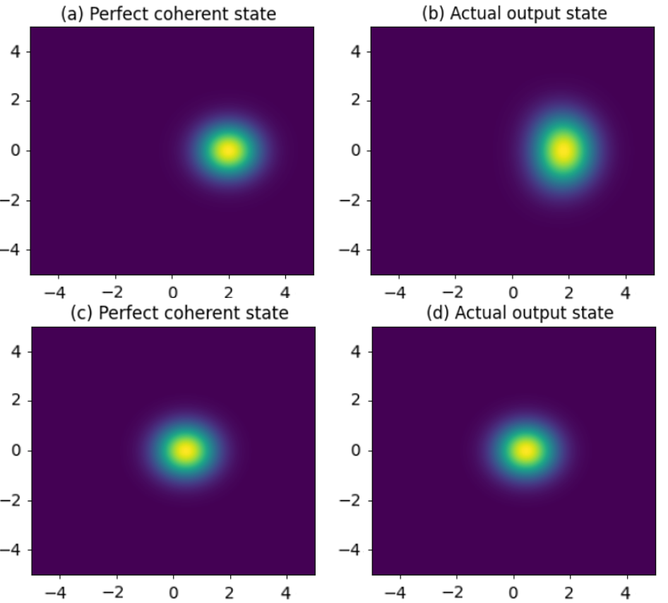
Figure 7: (a) The Wigner function of a coherent state with intensity $\mu=2$. (b) The Wigner function of $\rho_{A}^{X}$ with intensity $\mu_{max}=2,\Delta_{\phi}=\pi/4$. (c) The Wigner function of a coherent state with intensity $\mu=0.1$. (d) The Wigner function of $\rho_{A}^{X}$ with intensity $\mu_{max}=0.1,\Delta_{\phi}=\pi/24$ (corresponding to $N=24$). We deliberately choose a large intensity and wide phase slice for the above two figures to illustrate the spread of phases for $\rho_{A}^{X}$ due to the finite size of the phase slice. For the below two figures with reasonable intensity and phase slice values, we can see that the state $\rho_{A}^{X}$ is very close to the perfect coherent state (and the Wigner functions are almost indistinguishable). The Wigner function plots are generated with the QuTiP library [54].

To visualize the state, we can plot out the Wigner function of $\rho_{A}^{X}$, as shown in Fig. 7, where we also plot the Wigner function of a coherent state with intensity fixed at $\mu_{max}$ for comparison (here $\mu_{max}=2|\alpha_{0}|^{2}$). In Fig. 7 (a)(b) we choose an extreme case of $\mu_{max}=2,\Delta_{\phi}=\pi/4$ to more clearly illustrate the mixed phases caused by sorting signals into phase slices of a finite size.

In Figs. 7 (c)(d) we choose a set of reasonable values $\mu_{max}=0.1,\Delta_{\phi}=(\pi/24)$ (which are similar to the parameters used in our simulations). As can be seen, the output signal state in the passive TF-QKD setup is actually quite similar to that of active TF-QKD. Here when $N=24$, the fidelity between $\rho_{A}^{X}$ and $\ket{\alpha}\bra{\alpha}$ is as high as approximately $99.97\%$, and even when $N=8$ the fidelity is still about $99.74\%$. This means that, the finite size of phase slices has little effect on the statistics measured by Alice and Bob (hence the key rate is not affected much), but rather is only a security concern, which we address by constructing the virtual local channels, as described in the previous section.

Appendix F Decoy Analysis Models

In this section we describe the models of decoy state analysis we used to generate the key rates in Fig. 5, including that of active TF-QKD, passive TF-QKD with infinite decoys, and passive TF-QKD with a finite number of decoys. Note that, throughout this paper, we focus our discussions on the scenario of infinite signals only, while finite-size effects will be a subject of future work. When use terms including “asymptotic” and “finite” here, we are referring to the number of decoys settings.

1. Active TF-QKD: we simply follow the practical protocol 3 from [23], i.e. CAL TF-QKD with signal states of phases $\{0,\pi\}$ in the X basis, and phase-randomized decoy states with various intensity settings in the Z basis. In our simulation, we consider the asymptotic case with infinite decoy settings, i.e. Alice and Bob have perfect knowledge of all the photon yields $Y_{m_{A}m_{B}}$. We calculate the key rate simply using the theoretical values for the yields. The full form of yields in the presence of channel polarization misalignment is shown in [23]). Here for simplicity we consider no polarization misalignment, in which case the yields can be simplified into:

$$Y_{k_{c},k_{d},m_{A}m_{B}}^{Z,p_{d}=0}= \sum_{k=0}^{m_{A}}{{m_{A}}\choose{k}}\sum_{l=0}^{m_{B}}{{m_{B}}\choose{l}}$$ (28)

$$\times{{\eta^{k+l}(1-\eta)^{m_{A}+m_{B}-k-l}(k+l)!}\over{2^{k+l}k!l!}}$$

$$-(1-\eta)^{m_{A}+m_{B}},$$

where $\eta$ is the channel loss between Alice (Bob) and Charlie. In the presence of dark count $p_{d}$, the corrected yields are

$$Y_{k_{c},k_{d},m_{A}m_{B}}^{Z}= (1-p_{d})\left[p_{d}(1-\eta)^{m_{A}+m_{B}}+Y_{m_{A}m_{B}}^{p_{d}=0}\right].$$ (29)

2. Passive TF-QKD with infinite decoys: For passive TF-QKD, we first consider the case of infinite decoy settings, where we again assume that we have perfect knowledge of all photon yields $Y_{m_{A}m_{B}}$ and use Eqs. 28 and 29. The external channel yields $Y_{m_{A}m_{B}}$ are further used in calculating the corrected yields $Y_{n_{A}n_{B}}$ in Eq. 2 when including the effect of local channels in Alice’s and Bob’s labs in the passive TF-QKD security analysis. The corrected yields are then combined with passive signal state statistics to calculate the key rate.

There is actually a slightly caveat here: for passive TF-QKD, since there is no active basis-switching and the same signal is used for X and Z bases (just with different post-selection/post-processing strategies), the decoy intensities are limited to the range of $\mu_{A}\in[0,\mu_{max}]$ and $\mu_{B}\in[0,\mu_{max}]$ and are capped by $\mu_{max}$, which is on the order of $\approx 0.01-0.12$ and needs to be small because the phase error rate estimation favors smaller signal intensities (which affect the cat state coefficients). This is different from the ideal infinite-decoy case for active TF-QKD, where the decoy intensities can in principle go up to infinity.

However, we still have the freedom to choose as many divisions (each of which can also be infinitesimally small so it is equivalent to using a fixed intensity value instead of a range) within $[0,\mu_{max}]$ as we want. This means that, in theory, we can still get an infinite number of linearly independent equations, which are sufficient to solve any arbitrarily large numbers of variables $Y_{m_{A}m_{B}}$ accurately, which justifies our usage of theoretical values of $Y_{m_{A}m_{B}}$ when calculating the key rate for infinite-decoy passive TF-QKD.

3. Passive TF-QKD with a finite number of decoy settings: Lastly, for practical passive TF-QKD using a finite number of decoy settings, we need to divide up the map of $\mu_{A},\mu_{B}$ into decoy regions (such as the ones shown in Fig. 2 (b)) and perform passive decoy analysis. Each region functions as one decoy setting, where we calculate the gain and the photon number distribution by integrating over each given region, similar to what is performed in passive decoy-state BB84 protocol [8, 9] . The average photon number distribution is:

$$\langle P_{k_{c},k_{d}}^{Z}(m_{A},m_{B})\rangle ={1\over{P_{S_{ij}}}}\iint_{S_{ij}}$$ (30)

$$P_{Poisson}(\mu_{A},m_{A})P_{Poisson}(\mu_{B},m_{B})$$

$$P_{int}(\mu_{A},\mu_{B})d\mu_{A}d\mu_{B},$$

For instance for a grid of $3\times 3$ square regions, the distribution for each setting $(a,b)$ (where $a,b=1,2,3$) is

$$\langle P_{k_{c},k_{d}}^{Z}(m_{A},m_{B})\rangle ={1\over{P_{S_{ij}}}}\int_{(a-1)\mu_{max}/3}^{a\mu_{max}/3}\int_{(b-1)\mu_{max}/3}^{b\mu_{max}/3}$$ (31)

$$P_{Poisson}(\mu_{A},m_{A})P_{Poisson}(\mu_{B},m_{B})$$

$$P_{int}(\mu_{A},\mu_{B})d\mu_{A}d\mu_{B},$$

where the Poissonian distribution is

$$P_{Poisson}(\mu,n)=e^{-\mu}{{\mu^{n}}\over{n!}}.$$ (32)

Once we have the set of observables $\{Q_{k_{c},k_{d},i,j}^{Z}\}$, as well as the photon number distributions for each $(m_{A},m_{B})$, we can list out the linear equations

$$Q_{k_{c},k_{d},i,j}^{Z}=\sum_{n_{A},n_{B}}\langle P_{k_{c},k_{d}}^{Z}(m_{A},m_{B})\rangle Y^{Z}_{{k_{c}},{k_{d}},m_{A}m_{B}},$$ (33)

from which we can estimate the upper bounds of $Y^{Z}_{{k_{c}},{k_{d}},m_{A}m_{B}}$ and use it to calculate the upper bound for the phase error rate $e_{k_{c},k_{d}}^{Z}$.

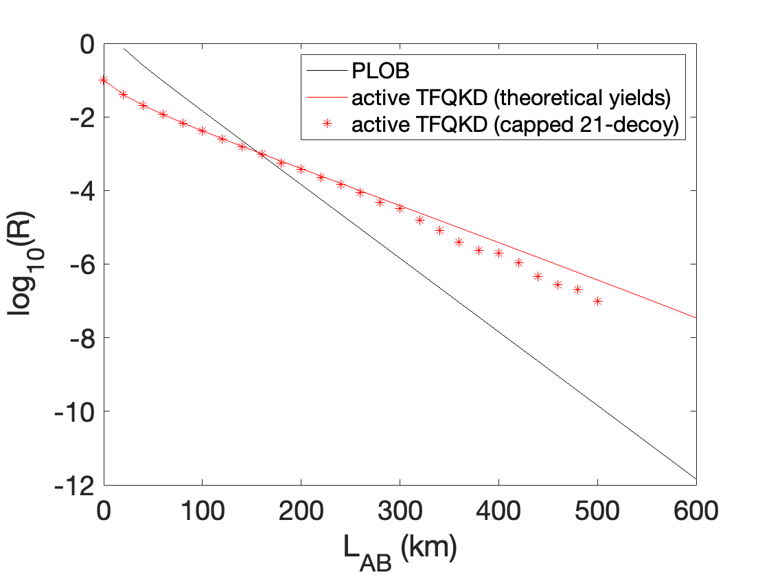
Figure 8: Comparison of key rates for active TF-QKD calculated with infinite number of decoys using theoretical values of yields and with decoys capped with a maximum intensity of $\mu_{max}\approx 0.1$ and solved with linear programming. We choose $\mu_{max}$ as the same optimal intensity for the case with theoretical yields. For the linear program, we choose as many number of decoys as numerically feasible in order to approach the asymptotic case (here we use $linspace(0,0.05,1)\times\mu_{max}$, where $linspace$ is an operator that returns an array of equidistant values between $0$ and $1$ with a step size of $0.05$, i.e. using $21\times 21$ decoy settings for Alice and Bob in total). No dark count or misalignment is introduced and the channel only contains loss. As can be seen, even with a large number of decoy settings and no noise, the key rate solved with linear programming is visibly lower at longer distances, illustrating the numerical instability caused by small coefficients in the linear program, which is a side-effect of using small decoy intensities.

Note that, as we mentioned above, the decoy intensities being capped to a small value does not fundamentally limit the asymptotic upper bound for the key rate of passive TF-QKD, since we can in principle still choose an infinite number of infinitesimally small decoy regions and solve for the yields with arbitrarily high precision. However, in practice, the smaller decoy intensity values may still cause some numerical instabilities for the linear solvers, due to the coefficients being small and neighboring linear equations having coefficient values that are rather close to each other. This means that small numerical inaccuracies might sometimes inadvertently cause some sets of linear constraints to be contradictory, making the linear program infeasible for some $Y_{m_{A}m_{B}}$ (in which case we have to upper-bound them to one, increasing the phase error rate and decreasing the key rate). We can illustrate this problem in Fig. 8 where we compare active TF-QKD with and without decoy intensities capped to a small value and solved with linear programming. The passive TF-QKD with three decoy settings suffers from similar numerical challenges, which means the numerically bounded key rate in Fig. 5 is slightly lower than what it could have theoretically been. Note that, however, the above problem not a theoretical limitation but just a numerical one, and e.g. scaling methods for the linear program can alleviate the problem to an extent (similar to the numerical problem and the methods to alleviate it as mentioned in Ref. [55]).

Also, experimentally, the smaller decoy intensities put a higher requirement on the accuracy of intensity measurement, but since the intensity measurement is performed on classical strong light, in principle we can have arbitrarily high accuracy for the measurements (albeit in reality this will be limited by the intensity of the laser diode, as well as the resolution and noise of the photodiode for detection). Again, this is not a theoretical limitation on our use of small decoy intensities, but rather an engineering one that can be lifted or at least alleviated with better equipment or experimental design.