Quantum Broadcast Channel Simulation
via Multipartite Convex Splitting

Abstract.

We show that the communication cost of quantum broadcast channel simulation under free entanglement assistance between the sender and the receivers is asymptotically characterized by an efficiently computable single-letter formula in terms of the channel’s multipartite mutual information. Our core contribution is a new one-shot achievability result for multipartite quantum state splitting via multipartite convex splitting. As part of this, we face a general instance of the quantum joint typicality problem with arbitrarily overlapping marginals. The crucial technical ingredient to sidestep this difficulty is a conceptually novel multipartite mean-zero decomposition lemma, together with employing recently introduced complex interpolation techniques for sandwiched Rényi divergences.

Moreover, we establish an exponential convergence of the simulation error when the communication costs are within the interior of the capacity region. As the costs approach the boundary of the capacity region moderately quickly, we show that the error still vanishes asymptotically.

1. Introduction

Quantum channel simulation endeavors to simulate a noisy quantum channel via a limited resource of noiseless channels and potentially other assistance such as, e.g., free entanglement. For simulating a point-to-point channel $\mathscr{N}_{A\to B}$ in the independent and identically distributed (i.i.d.) setting, Bennett et al. showed that under free entanglement-assistance the amount of asymptotic classical communication rate needed is equal to the quantum mutual information of channel [1, 2, 3]

$$I(\mathscr{N}_{A\to B}):=\sup_{\rho}I(B:R)_{(\mathscr{N}\otimes\mathrm{id})\left(\psi^{\rho}\right)},$$ (1.1)

where the maximum ranges over all input states $\rho_{A}$, $\psi_{AR}^{\rho}$ is a purification of $\rho_{A}$ by a reference system $R$, and $I$ denotes the quantum mutual information. Notably, the aforementioned classical communication cost coincides with the entanglement-assisted classical channel capacity [4, 1, 5]. Hence, from both operational and information-theoretic perspectives, point-to-point quantum channel simulation may be viewed as a reverse task of the quantum version of Shannon’s celebrated noisy coding theorem for simulating a noiseless channel via a noisy channel [6]. Accordingly, such a result is also termed the Quantum Reverse Shannon Theorem.

At first glance, one may wonder why to lavish noiseless channels on simulating the noisy one. To answer this question, firstly, the noisy coding theorem in conjunction with the Quantum Reverse Shannon Theorem lead us to characterizing resource inter-conversion [7, 8], e.g. finding the capacity of simulating a channel $\mathscr{N}$ from an arbitrary channel $\mathscr{M}$ in the presence of pre-shared entanglement in terms of a single quantity. Secondly, for the classical and classical-quantum special case, the channel simulation task may date back to the earlier studies on correlation generations [9, 10, 11, 12, 13, 8, 14], and channel resolvability [15, 16, 17, 18, 13, 19, 20, 21, 22, 23], which deliver applications to wiretap channel coding [24, 25, 26, 27, 28, 29], communication complexity of correlation [30], and measurement compression [31, 32, 33, 34]. Further information-theoretic applications include strong converse theorems [31, 1, 2], lossy data compression [31, 35, 36, 37], local purity distillation [38, 39, 40, 41], and entanglement distillation [42]. We refer the readers to [1, 2, 33, 14, 43] for more comprehensive reviews on this topic. It is worth mentioning that many of the above-mentioned works presume the input source to the channel to be fixed. Nonetheless, we will consider channel simulation under arbitrary sources; that is, we aim for a channel simulation result that works for the worst-case input scenario.

Notwithstanding the recent advances on point-to-point quantum channel simulation [3, 44, 45, 46], the asymptotic capacity region of general quantum broadcast channel simulation was left unknown prior to the present work. Broadcast channels [47, 48, 49, 50, 51, 52] are arguably one of the most simplest and practical network models in multi-user coding settings. This setting comprises a base station that wants to transmit down-link information to numerous and separate user equipments that only have their own local decodability. However, despite considerable efforts, the capacity region for a two-receiver broadcast channel coding is still unknown. On the reverse side of channel simulation, somewhat surprisingly, the capacity region for classical broadcast channel simulation under common randomness-assistance has recently been characterized in [43]. This naturally leads to a question:

“Can one obtain the capacity region for quantum broadcast channel simulation under free entanglement-assistance?”

Unfortunately, multi-user tasks are challenging in the fully quantum setting, since they are closely related to a serious technical barrier, the so-called quantum joint typicality [62] or simultaneous smoothing conjecture [63], and more generally the quantum marginal problem [64]. Consequently, previously only specialized scenarios of broadcast channel simulation could be handled. This includes the fixed i.i.d. input case via time sharing methods [65, 66], isometric broadcast channels [67] (see also[66]), and the recent result [43] on classical broadcast channels.

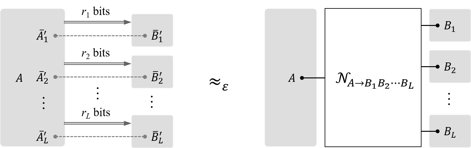
Figure 1. Depiction of an $L$-receiver quantum broadcast channel simulation. The Sender holds system $A$ and share free entanglement with $L$ receivers. By sending $r_{1}$, $r_{2}$, $\ldots$, $r_{L}$ bits of classical information to each receiver and local quantum operation at each receiver, the resulting transformation is close to an $L$-receiver quantum broadcast channel $\mathscr{N}_{A\to B_{1}B_{2}\ldots B_{L}}$ (in diamond norm). Note that each gray-shaded region is only allowed to perform local quantum operation.

In this paper, we establish the capacity region of general quantum broadcast channel simulation under free entanglement-assistance by circumventing the aforementioned obstacles around the quantum joint typicality conjecture. Taking the two-receiver broadcast channel $\mathscr{N}_{A\to B_{1}B_{2}}$ as an example, we show that the channel simulation is asymptotically achievable if and only if the classical communication costs $r_{1}$ and $r_{2}$ from the sender to each of two receivers (see Figure 1) satisfy

$$\left\{(r_{1},r_{2})\in\mathds{R}^{2}:r_{1}+r_{2}\geq I(\mathscr{N}_{A\to B_{1}B_{2}}),\,r_{1}\geq I(\mathscr{N}_{A\to B_{1}}),\,r_{2}\geq I(\mathscr{N}_{A\to B_{2}})\right\},$$ (1.2)

where the sum-rate is constrained by the bipartite mutual information of channel $\mathscr{N}_{A\to B_{1}B_{2}}$ [68, 69] (see the precise definition in Eq. (2.13)). Notably, we do not rely on the time-sharing technique and the capacity region for arbitrary $L$ receivers can be obtained as well (Theorem 5). Our proof techniques build on a conceptually new version of the multipartite convex-split lemma, a corresponding multipartite Quantum State Splitting protocol, and the (by now standard) Post-Selection Technique [70]. As our approach gets around a generic instance of the quantum joint typicality conjecture with arbitrarily overlapping marginals, we believe that it may serve as a general recipe for fully quantum network information-theoretic tasks.

Convex splitting was introduced by Anshu et al. in [71] (see also [72, 73]), which originates from the idea of rejection sampling in statistics [74, 75, 76], and it has an ample of applications in quantum information theory. In this paper, we generalize it to a conceptually new multipartite version and establish an one-shot error exponent bound. Taking the bipartite version as an illustration, assume that there are $M$ independent and identical copies of registers $A$’s, $K$ copies of registers $B$’s, and a single register $E$. Now the overall system is prepared in a way that register $E$ is correlated to the $m$-th register $A$ and the $k$-th register $K$ uniformly at random (see Figure 2). We then prove a tight one-shot bound on the trace distance between such a joint state and the all-tensor-product state (i.e. all of the systems $A$’s, $B$’s, and $E$ are decoupled) in terms of a generalized quantum Rényi information [77, 78, 79] (Theorem 3.1). The additivity of the Rényi information then immediately gives us a rate region for $M$ and $K$, for which the trace distance decreases exponentially in the asymptotic limit. This thus can be viewed as a bipartite generalization of the unipartite convex splitting by part of the authors [73]. To establish the result and avoid the need of the simultaneous smoothing, we introduce a key ingredient of a decomposition map, the multipartite mean-zero decomposition lemma (Lemma 3.1 & Lemma 3.2). We remark that a similar idea is independently proposed by Colomer Saus and Winter for deriving multipartite quantum decoupling theorems, termed the telescoping trick in their work [81].

An immediate application of the multipartite convex-split lemma is the multipartite version of Quantum State Splitting [65, 66] also termed mother protocol in its original (non-multipartite) form [82]. The goal is to transfer the systems $A_{1}^{\prime}$, $A_{2}^{\prime}$, $\ldots$, $A_{L}^{\prime}$ initially with Alice, to Bob, while the entanglement between all of Alice’s original systems $A$ and an inaccessible reference system $R$ is preserved. Given any classical communication cost consumed in the protocol, we obtain an one-shot error exponent bound on how well the protocol is performed.

Armed with multipartite Quantum State Splitting, we demonstrate how to combine the Post-Selection Technique [70] (as used in point-to-point quantum channel simulation [3]) and the quantum sandwiched information (Lemmas 2 and 2), to establish a one-shot error exponent bound for multipartite quantum broadcast channel simulation (Theorem 5) with diamond norm [83, 84] as an error criterion. We note that such a one-shot bound not only leads to the optimal achievable rate region in the i.i.d. setting; it also guarantees that the error of channel simulation decreases exponentially fast in the number of blocklength $n$ whenever the rate vector of communication costs is in the interior of the capacity region. Furthermore, we show the achievability part of a moderate deviation result [85, 86]. Namely, the error of simulation will vanish asymptotically, even though the rate vector converges to the boundary of the capacity region (Proposition 5).

Last but not least, let us point out some distinctive features of our results. The established multipartite convex splitting (Theorem 3.2) and multipartite Quantum State Splitting (Theorem 3) are one shot, in the sense that no mathematical constraint such as the i.i.d. assumption is needed. As for quantum broadcast channel simulation, we require the i.i.d. structure for the underlying channel to simulate. Our result (Theorem 5) is therefore non-asymptotic and for any finite blocklength, i.e. the assumption of infinitely large blocklength is not required. The reason behind our results is that we do not employ time-sharing techniques [48, Proposition 4.1], as this is not possible for the one-shot or finite blocklength setting (as pointed out even in classical network information theory [87, Remark 3]; see also [88]). By its nature, we believe that the proposed one-shot analysis, and in particular the multipartite mean-zero decomposition lemma (Lemma 3.2), could be a generic solution to problems in quantum network information theory.

The paper is structured in the following. We present an overview of our technical results in Section 1.1, and Section 1.2 contains discussions of related work. Notation and definitions for information measures are introduced in Section 2. Section 3 is devoted to establishing the multipartite convex splitting. The multipartite Quantum State Splitting achievability result is derived in Section 4. We give the proof of quantum broadcast channel simulation in Section 5. Some technical lemmas are left to the Appendices A and B.

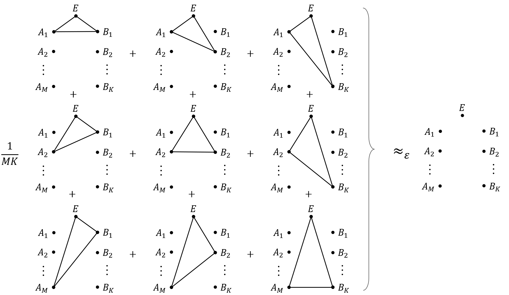
Figure 2. Depiction of a bipartite convex splitting. On the right part, each isolated dot represents an independent quantum system, and hence the overall state is product. On the left part, solid lines connected each system is a tripartite (correlated) state, while the other systems are left isolated. When $M$ and $K$ are sufficiently large (see Theorem 3.1), then the statistical mixture of the left part is close to the right part of product state (in trace norm).

1.1. Overview of Results

Our results are summarized below.

1. Multipartite convex splitting: For readability, we first present the result of the bipartite convex splitting. Let $\rho_{ABE}$, $\tau_{A}$, $\tau_{B}$ be states and let $M$ and $K$ be integers. The trace distance (i.e. trace norm divided by two) between the random mixture

   $$\frac{1}{MK}\sum_{m,k}\rho_{A_{m}B_{k}E}\bigotimes_{\bar{m}\neq m,\,\bar{k}\neq k}\tau_{A_{\bar{m}}}\otimes\tau_{B_{\bar{k}}}$$ (1.3)

   and the product state $\tau_{A}^{\otimes M}\otimes\tau_{B}^{\otimes K}\otimes\rho_{E}$ is upper bounded by (Theorem 3.1)

   $$2\cdot\,2^{-E_{\log MK}(\rho_{ABE}\,\|\,\tau_{A}\otimes\tau_{B})}+2^{-E_{\log M}(\rho_{AE}\,\|\,\tau_{A})}+2^{-E_{\log K}(\rho_{BE}\,\|\,\tau_{B})},$$ (1.4)

   where the error-exponent function

   $$E_{r}(\rho_{AE}\,\|\,\tau_{A}):=\sup_{\alpha\in[1,2]}\frac{\alpha-1}{\alpha}\left(r-I_{\alpha}(\rho_{AE}\,\|\,\tau_{A})\right)$$ (1.5)

   is the Fenchel–Legendre transform of the Rényi information [79]

   $$I_{\alpha}(\rho_{AE}\,\|\,\tau_{A}):=\inf_{\sigma_{E}}D_{\alpha}(\rho_{AE}\,\|\,\rho_{A}\otimes\sigma_{E})$$ (1.6)

   and $D_{\alpha}(\rho\,\|\,\sigma):=\frac{1}{\alpha-1}\log\operatorname{Tr}\left[(\sigma^{\frac{1-\alpha}{2\alpha}}\rho\sigma^{\frac{1-\alpha}{2\alpha}})^{\alpha}\right]$ is the quantum sandwiched Rényi divergence [77, 78]. Moreover, the three error exponents in Eq. (1.4) are all positive if and only if

   $$\begin{cases}&\log MK>I_{1}(\rho_{ABE}\,\|\,\tau_{A}\otimes\tau_{B})\\ &\log M>I_{1}(\rho_{AE}\,\|\,\tau_{A})\\ &\log K>I_{1}(\rho_{BE}\,\|\,\tau_{B})\\ \end{cases}.$$ (1.7)

   This then gives us an achievable rate region for a bipartite convex splitting.

   The result generalizes to arbitrary $L$-party case. Let $\rho_{A_{1}A_{2}\ldots A_{L}E}$ and $\tau_{A_{\ell}}$ be states and $M_{\ell}$ be an integer for each $\ell\in\{1,2,\ldots,L\}=:[L]$. The trace distance between the random mixture

   $$\frac{1}{M_{1}\cdots M_{L}}\sum_{m_{\ell}\in[M_{\ell}],\,\ell\in[L]}\rho_{A_{1,m_{1}}\cdots A_{L,m_{L}}E}\bigotimes_{\bar{m}_{\ell}\in[M_{\ell}]/\{m_{\ell}\},\,\ell\in[L]}\tau_{A_{\ell,\bar{m}_{\ell}}}$$ (1.8)

   and the product state $\bigotimes_{\ell\in[L]}\tau_{A}^{\otimes M_{\ell}}\otimes\rho_{E}$ is upper bounded by (Theorem 3.2)

   $$\sum_{\varnothing\neq S\subseteq[L]}2^{|S|}\cdot 2^{-E_{\log M_{S}}\left(\rho_{A_{S}E}\,\|\,\tau_{A_{S}}\right)},$$ (1.9)

   where $A_{S}$ denotes systems $A_{\ell}$ for all $\ell\in S$, and $M_{S}:=\prod_{\ell\in S}M_{\ell}$. Again, the achievable rate region is given by

   $$\left\{(M_{1},M_{2},\ldots,M_{L}):\log M_{S}>I_{1}(\rho_{A_{S}}\,\|\,\tau_{A_{S}}),\,\forall S\subseteq[L]\right\}.$$ (1.10)

2. Multipartite Quantum State Splitting: Let $\rho_{AA_{1}^{\prime}A_{2}^{\prime}\ldots A_{L}^{\prime}R}$ be a pure state holding by Alice and an inaccessible reference system $R$. Suppose that Alice and the $\ell$-th Receiver share many-copies of entangled state $|\tau\rangle_{\bar{A}_{\ell}^{\prime}\bar{B}_{\ell}}$, where $\bar{A}_{\ell}^{\prime}\cong\bar{B}_{\ell}\cong A_{\ell}^{\prime}$. The goal of an $L$-party Quantum State Splitting is to transfer each system $A_{\ell}^{\prime}$ to the $\ell$-th Receiver via $r_{\ell}$ bits of classical communication. Then, the error in terms of trace distance is upper bounded by (Theorem 3)

   $$\sqrt{\sum\nolimits_{\varnothing\neq S\subseteq[L]}2^{|S|}\cdot 2^{-E_{r_{S}}\left(\rho_{A_{S}^{\prime}R}\,\|\,\tau_{A_{S}^{\prime}}\right)}},$$ (1.11)

   where $r_{S}:=\sum_{\ell\in S}r_{\ell}$. Moreover, the error exponents are all positive if and only if for all $S\subseteq[L]$ ,

   $$r_{S}>I_{1}\left(\rho_{A_{S}^{\prime}R}\,\|\,\tau_{A_{S}^{\prime}}\right).$$ (1.12)

3. Quantum Broadcast Channel Simulation: Consider a general $L$-receiver quantum broadcast channel $\mathscr{N}_{A\to B_{1}B_{2}\ldots B_{L}}$, and free entanglement is present between Sender and $L$ Receivers. By sending $nr_{\ell}$ bits of classical information to the $\ell$-th Receiver, respectively, the simulated channel is close to $\mathscr{N}_{A\to B_{1}B_{2}\ldots B_{L}}^{\otimes n}$ in diamond norm [83, 84] with error at most (Theorem 5)

   $$\varepsilon_{n}\leq k_{n}\cdot\sqrt{\sum\nolimits_{\varnothing\neq S\subseteq[L]}2^{|S|}\cdot 2^{-nE_{r_{S}}(\mathscr{N}_{A\to B_{S}})}},$$ (1.13)

   where $B_{S}$ denotes the systems $B_{\ell}$ for all $\ell\in S$, and $k_{n}$ is a polynomial pre-factor depending on $L$ and the dimension of the input space. The function $E_{r_{S}}(\mathscr{N}_{A\to B_{S}})$ is the Fenchel–Legendre transform of $\sup_{\psi_{AR}}I_{\alpha}(\mathscr{N}_{A\to B_{S}}(\psi_{AR})\,\|\,\mathscr{N}_{A\to B_{S}}(\psi_{A}))$. Via a minimax identity (Proposition 2), it is equal to the error exponent corresponding to the worst-case purification $\psi_{AR}$. We remark that this result holds for any finite-blocklength $n$. The achievability result given in Eq. (1.13) leads us a lower bound on the overall error exponent (Proposition 5)

   $$\liminf_{n\to\infty}-\frac{1}{n}\log\varepsilon_{n}\geq\frac{1}{2}\min_{\varnothing\neq S\subseteq[L]}E_{r_{S}}\left(\mathscr{N}_{A\to B_{S}}\right).$$ (1.14)

   Then, we show that the capacity region of the broadcast channel simulation is given by (Theorem 5)

   $$\left\{(r_{1},r_{2},\ldots,r_{L}):\sum\nolimits_{\ell\in S}r_{\ell}\geq I(\mathscr{N}_{A\to B_{S}}),\forall S\subseteq[L]\right\}.$$ (1.15)

   The achievability in Eq. (1.13) also implies an achievability of the moderate deviation result [85, 86] as follows. For any subsets $\varnothing\neq S\subseteq[L]$, assume that the rates satisfy $\sum_{\ell\in S}r_{\ell,n}-I(\mathscr{N}_{A\to B_{S}})=\Theta(n^{-t})$ for some $t\in(0,\nicefrac{{1}}{{2}})$. That is, the $L$-tupe rate asymptotically converges to the boundary of the capacity region at certain speed. Then, we show that the error $\varepsilon_{n}$ of simulation still vanishes asymptotically (Proposition 5)

   $$\varepsilon_{n}\leq O\left(2^{-n^{1-2t}}\right)\to 0.$$ (1.16)

1.2. Related Work

The time reversal of Quantum State Splitting corresponds to coherent Quantum State Merging [82]. Further, a variant thereof, termed non-coherent Quantum State Merging was proposed by Horodecki et al. in [89, 90]. For the latter, one gives free LOCC and quantifies the entanglement needed to achieve the task of Quantum State Merging, whereas for the former one gives free entanglement and quantifies the communication requirements. The multipartite version of non-coherent Quantum State Merging was already studied in [90] as well, which then corresponds to the task of fully quantum distributed compression. We note that this multipartite Quantum State Merging result relies on time-sharing techniques [48, Proposition 4.1], meaning that once the the (simple) corner points of the capacity region are achieved, time sharing leads to the convex hull of them. Subsequently, the need of time sharing was removed with the use of chained typicality projectors [91, 62], that work for this special task because of the non-overlapping structure of the relevant quantum marginals. Moreover, we believe that these results could be lifted to the one-shot setting by means of the techniques from [63] and using the minimax smoothing from [92] even to tight cost functions in terms of smooth conditional min-entropy. However, working instead with the coherent Quantum State Merging task, it is unclear to us how to transform these entanglement cost functions to communication cost functions, in a way that retains joint smoothing and allows to later apply the Post-Selection Technique for quantum broadcast channel simulation. In short, for multipartite coherent Quantum State Merging one needs to solve an instance of the joint smoothing problem with overlapping marginals, whereas for multipartite non-coherent Quantum State Merging one gets away with non-overlapping marginals (becaus of the different structure of the cost function).

The technique of (unipartite) convex splitting was introduced by Anshu et al. in [71, 72]. The idea originated from rejection sampling in statistics [74], [75, Chapter 2.3], [76], and one of its specialized cases dates back to the classical soft covering by Wyner et al. [11, 15, 16, 93, 94, 95, 19, 28, 96, 26, 97, 23, 98]. It was recently generalized to an one-shot error-exponent result by parts of the authors [73]. The bipartite classical convex-split lemma — for which all the density operators share the same eigenbasis — was shown in [72, Fact 7]. Its straightforward generalization to the multipartite version was shown in [43, Lemma 39], which is the key lemma for showing classical broadcast channel simulation.

A bipartite quantum convex-split lemma was shown in [67, Lemma 2]. However, it is not clear to us whether this would lead to the optimal achievable rate region in the i.i.d. setting. In fact, [67, Theorem 4] provides an asymptotic i.i.d. analysis with an assumption that the whole joint state, i.e. $\rho_{ABE}$ in Eq. (1.4), is pure. To the best of our knowledge, this will only give an isometric broadcast channel simulation (see also[66]), rendering the simulation of general quantum broadcast channels previously open. On the other hand, a “bipartite” convex-split lemma was also shown in [99], wherein the system $E$ is absent. We remark that a multipartite convex-split lemma with the presence of system $E$ is crucial for the multipartite Quantum State Splitting and quantum broadcast channel simulation since the system $E$ plays the role of the reference system $R$ with which we want to protect the entanglement.

Indeed, establishing a one-shot achievability lemma for bipartite or multipartite settings that will yield the right achievable rate region is the central problem in quantum network information theory [64, 63, 90, 91, 62, 100, 101]. Our breakthrough here is to introduce a mean-zero decomposition lemma (Lemma 3.1) such that we can generally bypass the simultaneous smoothing/interpolation obstacles in the fully quantum setting. Taking the bipartite convex splitting as an example. The established one-shot bound in Eq. (1.4) immediately implies the achievable region given in Eq. (1.7). Hence, no sophisticated tools in asymptotic equipartition property such as typical projection onto subsystems, gentle measurement lemma [102], and the second-order asymptotics are needed. On the contrary, only the additivity of Rényi information is needed.

2. Notation and Information Quantities

Throughout this paper, the underlying Hilbert spaces associated to quantum registers/systems $A$, $B$, $C$, $\ldots$ are denoted by sans-serif fonts $\mathsf{A}$, $\mathsf{B}$, $\mathsf{C}$, $\ldots$, et cetera. The set of density operators (i.e. positive semi-definite operators with unit trace) and bounded operators on $\mathsf{A}$ are denoted by $\mathcal{S}(\mathsf{A})$ and $\mathcal{B}(\mathsf{A})$, respectively. The notation $|\mathsf{A}|$ stands for the dimension of Hilbert space $\mathsf{A}$. For a density operator $\rho_{A}$ or a bounded operator $X_{A}$ with subscript $A$, we mean the operator is on the Hilbert space $\mathsf{A}$ and often as the corresponding marginal of a multippartite operator $X$. We will use the term density operator and quantum state interchangeably in this paper.

For any $X\in\mathcal{B}(\mathsf{A})$ and , we define $\|X\|_{p}:=\left(\operatorname{Tr}[|X|^{p}]\right)^{\nicefrac{{1}}{{p}}}$ for $p>0$. We use $\mathds{N}$ and $\mathds{R}$ to denote positive integers and real numbers. For any positive integer $M\in\mathds{N}$, we shorthand the set $[M]:=\{1,2,\ldots,M\}$. We denote $\mathrm{id}_{R}:\mathcal{B}(\mathsf{R})\to\mathcal{B}(\mathsf{R})$ as the canonical identity map on $\mathsf{R}$, and denote $\mathrm{id}_{R}$ as the identity operator on $\mathsf{R}$. For any linear map $\mathscr{N}_{A\to B}:\mathcal{B}(\mathsf{A})\to\mathcal{B}(\mathsf{B})$, we define the diamond norm [83, 84] as

$$\left\|\mathscr{N}\right\|_{\diamond}:=\sup_{\left\lVert{{\rho_{AR}}}\right\lVert_{1}=1}\left\|\mathscr{N}_{A\to B}\otimes\mathrm{id}_{R}(\rho_{AR})\right\|_{1},$$ (2.1)

where $\mathsf{R}\cong\mathsf{A}$.

For any $\alpha\in(0,1)\cup(1,\infty)$, we define the order-$\alpha$ sandwiched quantum Rényi divergence $D_{\alpha}$ [77, 78] for density operator $\rho\in\mathcal{S}(\mathsf{A})$ and positive semi-definite $\sigma\in\mathcal{B}(\mathsf{A})$ as

$$D_{\alpha}(\rho\,\|\,\sigma) :=\frac{\alpha}{{\alpha}-1}\log\left\|\sigma^{\frac{1-\alpha}{2\alpha}}\rho{\sigma}^{\frac{1-\alpha}{2\alpha}}\right\|_{{\alpha}},$$ (2.2)

provided that the support of $\rho$ is contained in that of $\sigma$; otherwise, it is defined to be positive infinity. We define a generalized sandwiched Rényi information [79] for a bipartite state $\rho_{AB}\in\mathcal{S}(\mathsf{A}\otimes\mathsf{B})$ and positive semi-definite $\tau_{A}\in\mathcal{B}(\mathsf{A})$ and the usual sandwiched Rényi information as

$$I_{\alpha}(\rho_{AB}\,\|\,\tau_{A}): =\inf_{\sigma_{B}\in\mathcal{S}(\mathsf{B})}D_{\alpha}(\rho_{AB}\,\|\,\tau_{A}\otimes\sigma_{B});$$ (2.3)

$$I_{\alpha}(A:B)_{\rho} :=I_{\alpha}(\rho_{AB}\,\|\,\rho_{A}).$$ (2.4)

Moreover, we define the order-$\alpha$ sandwiched Rényi information for a quantum channel (i.e. completely positive and trace-preserving map) $\mathscr{N}_{A\to B}$ as

$$I_{\alpha}(\mathscr{N}_{A\to B}):=\sup_{\psi_{AR}}I_{\alpha}(B:R)_{(\mathscr{N}_{A\to B}\otimes\mathrm{id}_{R})(\psi)}.$$ (2.5)

Here and throughout this paper, $\sup_{\psi_{AR}}$ denotes maximizing over all pure states $\psi_{AR}\in\mathcal{S}(\mathsf{A}\otimes\mathsf{R})$ and $\mathsf{R}\cong\mathsf{A}$.

Remark .

If $|\mathsf{B}|<\infty$, then by the compactness of $\mathcal{S}(\mathsf{B})$, lower semi-continuity of the sandwiched Rényi divergence in its second argument [104], and the extreme value theorem, the minimum in Eq. (2.3) can be attained. An iterative algorithm with convergence guarantees was provided in [105]. In this paper, although we do not necessary impose the finite-dimensional assumption on the Hilbert space (especially for the output space), the minimum in Eq. (2.3) can also be attained.

As $\alpha\to 1$, the above quantities converge monotonically to the Umegaki’s quantum relative entropy [106],[107, Lemma 3.5], the generalized mutual information, the usual quantum mutual information, and the quantum mutual information of channel, respectively:

$$\lim_{\alpha\to 1}D_{\alpha}(\rho\,\|\,\sigma) =D(\rho\,\|\,\sigma):=\operatorname{Tr}\left[\rho(\log\rho-\log\sigma)\right],$$ (2.6)

$$\lim_{\alpha\to 1}I_{\alpha}(\rho_{AB}\,\|\,\tau_{A}) =I(\rho_{AB}\,\|\,\tau_{A}):=D(\rho_{AB}\,\|\,\tau_{A}\otimes\rho_{B}),$$ (2.7)

$$\lim_{\alpha\to 1}I_{\alpha}(A:B)_{\rho} =I(A:B)_{\rho}:=D(\rho_{AB}\,\|\,\rho_{A}\otimes\rho_{B}),$$ (2.8)

$$I(\mathscr{N}_{A\to B}) :=\sup_{\psi_{RA}}I(B:R)_{(\mathscr{N}_{A\to B}\otimes\mathrm{id}_{R})(\psi)}.$$ (2.9)

The above information quantities naturally extend to the multipartite setting (where system $A$ now has, say $L\in\mathds{N}$, subsystems). We define a multipartite sandwiched Rényi information for a multipartite state $\rho_{A_{1}A_{2}\ldots A_{L}E}\in\mathcal{S}(\mathsf{A}_{1}\otimes\mathsf{A}_{2}\otimes\cdots\otimes\mathsf{A}_{L}\otimes\mathsf{E})$ and a quantum broadcast channel $\mathscr{N}_{A\to B_{1}B_{2}\ldots B_{L}}:\mathcal{S}(\mathsf{A})\to\mathcal{S}(\mathsf{B}_{1}\otimes\mathsf{B}_{2}\otimes\cdots\otimes\mathsf{B}_{L})$ as

$$I_{\alpha}\left(A_{1}:A_{2}:\cdots:A_{L}:E\right)_{\rho} :=I_{\alpha}\left(\rho_{A_{1}A_{2}\ldots A_{L}E}\,\|\otimes_{\ell\in[L]}\rho_{A_{\ell}}\right);$$ (2.10)

$$I_{\alpha}(\mathscr{N}_{A\to B_{1}B_{2}\ldots B_{L}}) :=\max_{\psi_{AR}}I_{\alpha}\left(B_{1}:B_{2}:\cdots:B_{L}:R\right)_{(\mathscr{N}\otimes\mathrm{id}_{R})(\psi)}.$$ (2.11)

In particular, we term

$$\lim_{\alpha\to 1}I_{\alpha}\left(A_{1}:A_{2}:\cdots:A_{L}:E\right)_{\rho} \equiv I\left(A_{1}:\cdots:A_{L}:E\right)_{\rho}:=D\left(\rho_{A_{1}\ldots A_{L}E}\,\|\otimes_{\ell\in[L]}\rho_{A_{\ell}}\otimes\rho_{E}\right)_{\rho},$$ (2.12)

$$I(\mathscr{N}_{A\to B_{1}B_{2}\ldots B_{L}}) :=\max_{\psi_{AR}}I\left(B_{1}:B_{2}:\cdots:B_{L}:R\right)_{(\mathscr{N}\otimes\mathrm{id}_{R})(\psi)}$$ (2.13)

as the multipartite quantum mutual information [68, 69] $I\left(A_{1}:\cdots:A_{L}:E\right)_{\rho}$ for state $\rho_{A_{1}A_{2}\ldots A_{L}E}$ and the quantum mutual information $I(\mathscr{N}_{A\to B_{1}B_{2}\ldots B_{L}})$ for quantum broadcast channel $\mathscr{N}_{A\to B_{1}B_{2}\ldots B_{L}}$, respectively.

We further define the relative entropy variance [108, 109] $V(\rho\,\|\,\sigma)$, mutual information variance ${V(A_{1}:\cdots:A_{L}:E)_{\rho}}$, and channel dispersion $V(\mathscr{N}_{A\to B_{1}B_{2}\ldots B_{L}})$ for a broadcast channel $\mathscr{N}_{A\to B_{1}B_{2}\ldots B_{L}}$ as

$$V(\rho\,\|\,\sigma) :=\operatorname{Tr}[\rho(\log\rho-\log\sigma)^{2}]-\left[D(\rho\,\|\,\sigma)\right]^{2};$$ (2.14)

$$V\left(A_{1}:\cdots:A_{L}:E\right)_{\rho} :=V\left(\rho_{A_{1}\ldots A_{L}E}\,\|\otimes_{\ell\in[L]}\rho_{A_{\ell}}\otimes\rho_{E}\right);$$ (2.15)

$$V(\mathscr{N}_{A\to B_{1}B_{2}\ldots B_{L}}) :=\sup_{\psi_{AR}:I(B_{1}:\cdots:B_{L}:R)_{(\mathscr{N}\otimes\mathrm{id}_{R})(\psi)}=I(\mathscr{N})}V(B_{1}:\cdots:B_{L}:R)_{(\mathscr{N}\otimes\mathrm{id}_{R})(\psi)}.$$ (2.16)

Below we collect several well-known properties of the generalized Rényi information. Essentially they all follow similarly as the special case $L=1$ [78, 107], [79, Lemma 7], [110, 23], and [46, Lemma 17].

[Properties of Rényi information] For any multipartite state $\rho_{A_{1}A_{2}\ldots A_{L}E}$ and $\tau_{A_{\ell}}\in\mathcal{S}(\mathsf{A}_{\ell})$, $\ell\in[L]$, and $\alpha\geq\nicefrac{{1}}{{2}}$, the sandwiched Rényi information satisfies the following properties.

1. (Monotone decreasing [78],[107, Lemma 4.6]) When ${\alpha}\to 1$,

   $$I_{\alpha}\left(\rho_{A_{1}A_{2}\ldots A_{L}E}\,\|\otimes_{\ell\in[L]}\tau_{A_{\ell}}\right)\searrow I\left(\rho_{A_{1}A_{2}\ldots A_{L}E}\,\|\otimes_{\ell\in[L]}\tau_{A_{\ell}}\right).$$ (2.17)

2. (Additivity [79, Lemma 7]) For any integer $n\in\mathds{N}$,

   $$I_{\alpha}\left(\rho_{A_{1}A_{2}\ldots A_{L}E}^{\otimes n}\,\|\otimes_{\ell\in[L]}\tau_{A_{\ell}}^{\otimes n}\right)=nI_{\alpha}\left(\rho_{A_{1}A_{2}\ldots A_{L}E}\,\|\otimes_{\ell\in[L]}\tau_{A_{\ell}}\right).$$ (2.18)

3. (Concavity in $\alpha$ [110, Theorem 11]) The following map is concave and upper semi-continuous on $(1,\infty)$:

   $$\alpha\mapsto\frac{1-\alpha}{\alpha}I_{\alpha}\left(\rho_{A_{1}A_{2}\ldots A_{L}E}\,\|\otimes_{\ell\in[L]}\tau_{A_{\ell}}\right).$$ (2.19)

4. (Concavity in $\psi$ [46, Lemma 17]) The following map is concave and upper semi-continuous on $\mathcal{S}(\mathsf{A})$:

   $$\rho_{A}\mapsto I_{\alpha}\left(B_{1}:B_{2}:\cdots B_{L}:R\right)_{\mathscr{N}_{A\to B_{1}B_{2}\ldots B_{L}}(\psi_{AR}^{\rho})},$$ (2.20)

   where $\psi_{AR}^{\rho}$ is a purification of $\rho_{A}$ and $\mathsf{R}\cong\mathsf{A}$.

The following Lemmas 2 and 2 will be used in Section 5 for broadcast channel simulation. We delay their proofs to Appendix A.

[Dimension bound] For any states $\rho_{ABC}\in\mathcal{S}(\mathsf{A}\otimes\mathsf{B}\otimes\mathsf{C})$, $\tau_{A}\in\mathcal{S}(\mathsf{A})$, and $\alpha>0$, we have

$$I_{\alpha}\left(\rho_{ABC}\,\|\,\tau_{A}\right)\leq I_{\alpha}\left(\rho_{AB}\,\|\,\tau_{A}\right)+\frac{2\alpha}{\alpha-1}\log|\mathsf{C}|.$$ (2.21)

[Convexity] Let $L$ be any integer and $\mathcal{I}$ be any finite set. Let $\rho_{A_{1}A_{2}\ldots A_{L}E}:=\sum_{i\in\mathcal{I}}p_{i}\rho_{A_{1}A_{2}\ldots A_{L}E}^{i}$ and $\tau_{A_{\ell}}=\sum_{i\in\mathcal{I}}p_{i}\tau_{A_{\ell}}^{i}$, $\ell\in[L]$ be statistical mixtures of states for any $p_{i}>0$, $\sum_{i\in\mathcal{I}}p_{i}=1$. Then, the following holds for every $\alpha\geq\nicefrac{{1}}{{2}}$,

$$\begin{split}I_{\alpha}(\rho_{A_{1}\ldots A_{L}E}\,\|\otimes_{\ell\in[L]}\tau_{A_{\ell}})&\leq\sum\nolimits_{i\in\mathcal{I}}p_{i}I_{\alpha}\left(\rho_{A_{1}\ldots A_{L}E}^{i}\,\|\otimes_{\ell\in[L]}\tau_{A_{\ell}}^{i}\right)+L\cdot H(\{p_{i}\}_{i\in\mathcal{I}})\\ &\leq\sum\nolimits_{i\in\mathcal{I}}p_{i}I_{\alpha}\left(\rho_{A_{1}\ldots A_{L}E}^{i}\,\|\otimes_{\ell\in[L]}\tau_{A_{\ell}}^{i}\right)+L\log|\mathcal{I}|.\end{split}$$ (2.22)

Here, $H(\{p_{i}\}_{i\in\mathcal{I}}):=-\sum_{i\in\mathcal{I}}p_{i}\log p_{i}$ denotes the Shannon entropy.

We introduce the error-exponent functions as the Fenchel–Legendre transform of the above Rényi information quantities, i.e. for any $r>0$,

$$E_{r}(\rho_{A_{1}A_{2}\ldots A_{L}B}\,\|\,\otimes_{\ell\in[L]}\tau_{A_{\ell}}) :=\sup_{\alpha\in[1,2]}\frac{\alpha-1}{\alpha}\left(r-I_{\alpha}(\rho_{A_{1}A_{2}\ldots A_{L}E}\,\|\,\otimes_{\ell\in[L]}\tau_{A_{\ell}})\right);$$ (2.23)

$$E_{r}(A_{1}:A_{2}:\cdots:A_{L}:E)_{\rho} :=E_{r}(\rho_{A_{1}A_{2}\ldots A_{L}E}\,\|\otimes_{\ell\in[L]}\rho_{A_{\ell}});$$ (2.24)

$$E_{r}(\mathscr{N}_{A\to B_{1}B_{2}\ldots B_{L}}) :=\sup_{\alpha\in[1,2]}\frac{\alpha-1}{\alpha}\left(r-I_{\alpha}(\mathscr{N}_{A\to B_{1}B_{2}\ldots B_{L}})\right).$$ (2.25)

We collect the known properties of the error-exponent function [111, 86, 112, 113, 23, 98], which are consequences of the the properties of the Rényi information given in Proposition 2. and the minimax theorem [114, §36]. [Properties of error-exponent function] For any multipartite state $\rho_{A_{1}A_{2}\ldots A_{L}B}$ and any quantum broadcast channel $\mathscr{N}_{A\to B_{1}B_{2}\ldots B_{L}}$, the error-exponent function satisfies the following properties.

1. (Positivity) For any $r>0$,

   $$E_{r}(\rho_{A_{1}A_{2}\ldots A_{L}B}\,\|\otimes_{\ell\in[L]}\tau_{A_{\ell}})>0 \Longleftrightarrow r>I(\rho_{A_{1}A_{2}\ldots A_{L}B}\,\|\otimes_{\ell\in[L]}\tau_{A_{\ell}});$$ (2.26)

   $$E_{r}(\mathscr{N}_{A\to B_{1}B_{2}\ldots B_{L}})>0 \Longleftrightarrow r>I(\mathscr{N}_{A\to B_{1}B_{2}\ldots B_{L}}).$$ (2.27)

2. (Additivity) For any integer $n\in\mathds{N}$ and $r>0$,

   $$E_{nr}\left(\rho_{A_{1}A_{2}\ldots A_{L}B}^{\otimes n}\,\|\otimes_{\ell\in[L]}\tau_{A_{\ell}}^{\otimes n}\right)=nE_{{r}}\left(\rho_{A_{1}A_{2}\ldots A_{L}B}\,\|\otimes_{\ell\in[L]}\tau_{A_{\ell}}\right).$$ (2.28)

3. (A minimax identity and saddle-point) Provided that the underlying Hilbert spaces are all finite dimensional, for any $r>0$, there exist a saddle-point $(\psi,\alpha)\in\mathcal{S}(\mathsf{A}\otimes\mathsf{R})\times[1,2]$[114, §36] such that

   $$E_{r}(\mathscr{N}_{A\to B_{1}B_{2}\ldots B_{L}}) =\inf_{\psi_{AR}}E_{r}(B_{1}:B_{2}:\cdots B_{L}:R)_{(\mathscr{N}\otimes\mathrm{id}_{R})(\psi)}$$ (2.29)

   $$=\frac{\alpha-1}{\alpha}\left(r-I_{\alpha}(B_{1}:B_{2}\cdots B_{L}:R)_{(\mathscr{N}\otimes\mathrm{id}_{R})(\psi)}\right).$$ (2.30)

4. (Limiting behavior) Provided that the underlying Hilbert spaces are all finite dimensional, then for any sequence $r_{n}:=I\left(\mathscr{N}_{A\to B_{1}B_{2}\ldots B_{L}}\right)+a_{n}$ satisfying $a_{n}\downarrow 0$, we have

   $$\liminf_{n\to\infty}\frac{E_{r_{n}}(\mathscr{N})}{a_{n}^{2}} \geq\frac{1}{2V(\mathscr{N}_{A\to B_{1}B_{2}\ldots B_{L}})}.$$ (2.31)

We delay the proof to Appendix A.

Remark .

Proposition 2-iii indicates that the error exponent of channel $E_{r}(\mathscr{N}_{A\to B_{1}B_{2}\ldots B_{L}})$ can be viewed as the error exponent $E_{r}(B_{1}:B_{2}:\cdots B_{L}:R)_{(\mathscr{N}\otimes\mathrm{id}_{R})(\psi)}$ for the output state with respect to the worst-case input $\psi_{AR}$.

3. Convex Splitting

In Ref. [73], part of the authors established a one-shot error-exponent bound for unipartite convex splitting, i.e. for any density operators $\rho_{AE}\in\mathcal{S}(\mathsf{A\otimes E})$ and $\tau_{A}\in\mathcal{S}(\mathsf{A})$, and $M\in\mathds{N}$,

$$\frac{1}{2}\left\|\frac{1}{M}\sum\nolimits_{m\in[M]}\rho_{A_{m}E}\bigotimes\nolimits_{\bar{m}\in[M]\setminus\{m\}}\tau_{A_{\bar{m}}}-\tau_{A}^{\otimes M}\otimes\rho_{E}\right\|_{1} \leq 2^{-E_{\log M}(\rho_{AE}\,\|\,\tau_{A})},$$ (3.1)

where $\rho_{A_{m}E}=\rho_{AE}$ and $\tau_{A_{m}}=\tau_{A}$ for all $m\in[M]$, and the error-exponent function $E_{\log M}$ is defined in Eq. (2.23). While this result is a neat application of complex interpolation, a straightforward generalization to the multipartite case does not give the Rényified quantities simultaneously. The key ingredient to bypass this difficulty is a mean-zero decomposition lemma that will be introduced later in Lemma 3.1 and Lemma 3.2. We remark that a similar idea is independently proposed by Colomer Saus and Winter for deriving multipartite quantum decoupling theorems, termed the telescoping trick in their work [81].

3.1. Bi-partite Convex Splitting

Let $\rho_{ABE}$ be a tripartite density operator in $\mathcal{S}(\mathsf{A\otimes B\otimes E})$, and let $\tau_{AB}$ be a bipartite density operator $\mathcal{S}(\mathsf{A\otimes B})$. Given integers $M$ and $K$, we define the density operator

$$\begin{split}\omega_{A_{1}\ldots A_{M}B_{1}\ldots B_{K}E}:=\frac{1}{MK}\sum_{(m,k)\in[M]\times[K]}\rho_{A_{m}B_{k}E}&\otimes\tau_{A_{1}}\otimes\tau_{A_{2}}\cdots\otimes\tau_{A_{m-1}}\otimes\tau_{A_{m+1}}\otimes\cdots\otimes\tau_{A_{M}}\\ &\otimes\tau_{B_{1}}\otimes\tau_{B_{2}}\cdots\otimes\tau_{B_{k-1}}\otimes\tau_{B_{k+1}}\otimes\cdots\otimes\tau_{B_{K}},\end{split}$$ (3.2)

where for each $m\in[M]$ and $k\in[K]$, we have the systems $A_{m}\cong A$, $B_{k}\cong B$ and the states $\rho_{A_{m}B_{k}}=\rho_{AB}$, $\tau_{A_{m}}=\tau_{A}$, and $\tau_{B_{k}}=\tau_{B}$. We use trace distance as the error criterion for bipartite convex splitting,

$$\begin{split}\Delta_{M,K}(\rho_{ABE}\,\|\,\tau_{AB})&:=\frac{1}{2}\left\|\omega_{A_{1}\ldots A_{M}B_{1}\ldots B_{K}E}-\tau_{A}^{\otimes M}\otimes\tau_{B}^{\otimes K}\otimes\rho_{E}\right\|_{1}.\end{split}$$ (3.3)

Given $p\geq 1$, recall that the Kosaki’s weighted $L_{p}$-norm with respective to a density operator $\sigma$ [115, 116] is defined as,

$$\begin{split}\left\|X\right\|_{p,\sigma}&:=\left(\operatorname{Tr}\left[\left|\sigma^{\frac{1}{2p}}X\sigma^{\frac{1}{2p}}\right|^{p}\right]\right)^{\nicefrac{{1}}{{p}}}\end{split}$$ (3.4)

and the associated noncommutative weighted $L_{p}$-space is denoted as $L_{p}(\sigma)=\left\{X:\|X\|_{p,\sigma}<\infty\right\}$. For two positive operators $X$ and $Y$ we introduce the notation of non-commutative quotient for $X$ over $Y$ as

$$\frac{X}{Y}:=Y^{-\frac{1}{2}}XY^{-\frac{1}{2}}.$$ (3.5)

Our approach (as in the unipartite convex splitting [73]) is to formulate the error $\Delta_{M}\left(\rho_{ABE}\,\|\,\tau_{AB}\right)$ as the weighted $L_{p}$ norm and estimate it via complex interpolation. We refer to [73, Appendix B] for a minimal introduction of complex interpolation needed for this paper and the readers are referred to [117] for more information on this topic . We start with rewriting the error quantity in Eq. (3.3) using non-commutative $L_{p}$-norm. Given a density operator $\tau_{AB}=\tau_{A}\otimes\tau_{B}$, we define the $\tau$-preserving conditional expectation

$$\mathrm{E}_{A}:\mathcal{B}(\mathsf{A})\to\mathcal{B}(\mathsf{A}),\;X_{A}\mapsto\operatorname{Tr}_{A}\left[\tau_{A}X_{A}\right]\cdot\mathds{1}_{A};$$

$$\mathrm{E}_{B}:\mathcal{B}(\mathsf{B})\to\mathcal{B}(\mathsf{B}),\;X_{B}\mapsto\operatorname{Tr}_{B}\left[\tau_{B}X_{B}\right]\cdot\mathds{1}_{B};$$

$$\mathrm{E}_{AB}:=\mathrm{E}_{A}\otimes\mathrm{E}_{B}:\mathcal{B}(\mathsf{A\otimes B})\to\mathcal{B}(\mathsf{A\otimes B}).$$ (3.6)

The following map is an key object in the bipartite analysis.

$$\begin{split}&T:\mathcal{B}(\mathsf{A\otimes B})\to\mathcal{B}(\mathsf{A\otimes B})\ ,\ T:=\mathrm{id}_{AB}-\mathrm{E}_{A}-\mathrm{E}_{B}+\mathrm{E}_{AB}.\end{split}$$ (3.7)

Here and in the following, $\mathrm{E}_{A}$ can be interpreted as $\mathrm{E}_{A}\otimes\mathrm{id}_{B}$ and similar for $\mathrm{E}_{B}$. We will shortly see how the map $T$ comes into play. Let us first state the following lemma that estimates its norm between $L_{p}$-spaces.

Let $\tau=\tau_{A}\otimes\tau_{B}\otimes\tau_{E}\in\mathcal{S}(\mathsf{A}\otimes\mathsf{B}\otimes\mathsf{E})$ be a tripartite product density operator and a map $T$ introduced in Eq. (LABEL:eq:tele). Then

$$\left\lVert{{T:L_{1}(\tau_{ABE})\to L_{1}(\tau_{ABE})}}\right\lVert\leq 4\hskip 2.84544pt,\hskip 2.84544pt\left\lVert{{T:L_{2}(\tau_{ABE})\to L_{2}(\tau_{ABE})}}\right\lVert\leq 2.$$

Proof.

We first argue for $L_{1}$. Note that $\mathrm{E}_{A}\mathrm{E}_{B}=\mathrm{E}_{B}\mathrm{E}_{A}=\mathrm{E}_{AB}$. By triangle inequality, it suffices to show both $\mathrm{E}_{A}$ and $\mathrm{E}_{B}$ are contraction. Indeed, consider the duality $L_{1}(\tau)^{*}=L_{\infty}(\tau)$, where the pairing is given the $\tau$-inner product

$$\langle X,Y\rangle_{\tau}=\operatorname{Tr}(X\tau^{1/2}Y\tau^{1/2})\hskip 2.84544pt.$$

Note that $\mathrm{E}_{A}$ is completely positive unital map, hence a contraction on $L_{\infty}(\tau)\cong\mathcal{B}(\mathsf{A\otimes B\otimes E})$ (equipped with usual operator norm). Also, as $\mathrm{E}_{A}$ is self-adjoint for $\tau$-inner product. Then

$$\left\lVert{{\mathrm{E}_{A}:L_{1}(\tau)\to L_{1}(\tau)}}\right\lVert=\left\lVert{{\mathrm{E}_{A}:=L_{\infty}(\tau)\to L_{\infty}(\tau)}}\right\lVert=1.$$

The same argument applies for $\mathrm{E}_{B}$. Thus we prove that $\left\lVert{{T:L_{1}\to L_{1}}}\right\lVert\leq 4$ by triangle inequality.

For $L_{2}$, we note that $\mathrm{E}_{A}$ is a $\tau$-preserving conditional expectation. That is, $\operatorname{Tr}[\tau\mathrm{E}_{A}(X)]=\operatorname{Tr}[\tau X]$ for all $X\in\mathcal{B}(\mathsf{A}\otimes\mathsf{B}\otimes\mathsf{E})$, and $\mathrm{E}_{A}^{2}=\mathrm{E}_{A}$ is a unital complete positive idempotent. In particular, $\mathrm{E}_{A}$ is a projection on $L_{2}(\tau)$. As $\mathrm{E}_{B}$ is a projection commute with $\mathrm{E}_{B}$, we have

$$X-\mathrm{E}_{A}(X)-\mathrm{E}_{B}(X)+\mathrm{E}_{AB}(X)=(X-\mathrm{E}_{A}(X))-\mathrm{E}_{B}(X-\mathrm{E}_{A}(X))\ .$$

Hence

$$\left\lVert{{X}}\right\lVert_{L_{2}(\tau)}\geq\left\lVert{{X-\mathrm{E}_{A}(X)}}\right\lVert_{L_{2}(\tau)}\geq\left\lVert{{\mathrm{E}_{B}(X)-\mathrm{E}_{AB}(X)}}\right\lVert_{L_{2}(\tau)}.$$

The second assertion follows from triangle inequality for $L_{2}(\tau)$. ∎

In the following, we use the short notation $A^{M}:=A_{1}\cdots A_{M}\cong A^{\otimes M}$ and $B^{K}:=B_{1}\cdots B_{K}\cong B^{\otimes K}$. Given $(m,k)\in[M]\times[K]$, we define the following maps

$$\pi_{m,k}: \;\mathcal{B}(\mathsf{A}\otimes\mathsf{B})\to\mathcal{B}(\mathsf{A}^{M}\otimes\mathsf{B}^{K})$$

$$\;\;X_{AB}\mapsto\mathds{1}_{A_{1}B_{1}}\otimes\cdots\otimes\mathds{1}_{A_{m-1}B_{k-1}}\otimes X_{A_{m}B_{k}}\otimes\mathds{1}_{A_{m+1}B_{k+1}}\otimes\cdots\otimes\mathds{1}_{A_{M}B_{K}};$$

$$\mathrm{E}_{A_{m}}: \;X_{A_{m}}\mapsto\operatorname{Tr}_{A_{m}}\left[\rho_{A_{m}}X_{A_{m}}\right]\cdot\mathds{1}_{A_{m}};$$

$$\mathrm{E}_{B_{k}}: \;X_{B_{k}}\mapsto\operatorname{Tr}_{B_{k}}\left[\rho_{B_{k}}X_{B_{k}}\right]\cdot\mathds{1}_{B_{k}};$$

$$\Theta:= \;\frac{1}{MK}\sum_{(m,k)\in[M]\times[K]}\pi_{m,k}$$

Here, the condition expectation $\mathrm{E}_{A_{m}}$ is only acting on the ${A}_{m}$ system while other systems remain unchanged; similarly for $\mathrm{E}_{B_{k}}$. It is clear that

$$\pi_{m,k}\mathrm{E}_{A}=\mathrm{E}_{A_{m}}\pi_{m,k}\ ,\pi_{m,k}\mathrm{E}_{B}=\mathrm{E}_{B_{k}}\pi_{m,k}\ ,\pi_{m,k}\mathrm{E}_{AB}=\mathrm{E}_{A_{m}B_{k}}\pi_{m,k}\hskip 2.84544pt.$$

Take $\tau_{ABE}=\tau_{A}\otimes\tau_{B}\otimes\sigma_{E}$ for an arbitrary density $\sigma_{E}\in\mathcal{S}(\mathsf{E})$. We have

$$\Delta_{M,K}\left(\rho_{ABE}\,\|\,\tau_{AB}\right) =\frac{1}{2}\left\|\omega_{A_{1}\ldots A_{M}B_{1}\ldots B_{K}E}-\tau_{A}^{\otimes M}\otimes\tau_{B}^{\otimes K}\otimes\rho_{E}\right\|_{1}$$ (3.8)

$$=\frac{1}{2}\left\|\frac{\omega_{A_{1}\ldots A_{M}B_{1}\ldots B_{K}E}}{\tau_{A^{M}B^{K}E}}-\mathds{1}_{A^{M}B^{K}}\otimes\frac{\rho_{E}}{\sigma_{E}}\right\|_{L_{1}(\tau_{A^{M}B^{K}E})}$$ (3.9)

$$=\frac{1}{2}\left\|\frac{1}{MK}\sum_{m,k}\pi_{m,k}\left(\frac{\rho_{ABE}}{\tau_{A}\otimes\tau_{B}\otimes\sigma_{E}}\right)-\mathds{1}_{A^{M}B^{K}}\otimes\frac{\rho_{E}}{\sigma_{E}}\right\|_{L_{1}(\tau_{A^{M}B^{K}E})}$$ (3.10)

$$=\frac{1}{2}\left\|\frac{1}{MK}\sum_{m,k}\pi_{m,k}\left(\frac{\rho_{ABE}}{\tau_{A}\otimes\tau_{B}\otimes\sigma_{E}}-\mathds{1}_{AB}\otimes\frac{\rho_{E}}{\sigma_{E}}\right)\right\|_{L_{1}(\tau_{A^{M}B^{K}E})}$$ (3.11)

$$=\frac{1}{2}\left\|\frac{1}{MK}\sum_{m,k}\pi_{m,k}\circ(\mathrm{id}_{AB}-\mathrm{E}_{AB})\left(\frac{\rho_{ABE}}{\tau_{A}\otimes\tau_{B}\otimes\sigma_{E}}\right)\right\|_{L_{1}(\tau_{A^{M}B^{K}E})}$$ (3.12)

$$=\frac{1}{2}\left\|\Theta\circ(\mathrm{id}_{AB}-\mathrm{E}_{AB})\left(\frac{\rho_{ABE}}{\tau_{A}\otimes\tau_{B}\otimes\sigma_{E}}\right)\right\|_{L_{1}(\tau_{A^{M}B^{K}E})}.$$ (3.13)

A key observation is that, for $X\equiv X_{ABE}=\frac{\rho_{ABE}}{\tau_{A}\otimes\tau_{B}\otimes\sigma_{E}}$, we can decompose in Eq. (3.13) into the following three terms:

$$(\mathrm{id}_{AB}-\mathrm{E}_{AB})(X)=X-\mathrm{E}_{AB}(X)=(X-\mathrm{E}_{A}X-\mathrm{E}_{B}X+\mathrm{E}_{AB}X)+(\mathrm{E}_{A}X-\mathrm{E}_{AB}X)+(\mathrm{E}_{B}X-\mathrm{E}_{AB}X)\hskip 2.84544pt.$$ (3.14)

Let us evaluate one of them:

$$\left\|\Theta(\mathrm{E}_{A}X-\mathrm{E}_{AB}X)\right\|_{L_{1}(\tau_{A^{M}B^{K}E})}$$

$$=\left\lVert{{\Theta\left(\mathds{1}_{A}\otimes\frac{\rho_{BE}}{\tau_{B}\otimes\sigma_{E}}-\mathds{1}_{AB}\otimes\frac{\rho_{E}}{\sigma_{E}}\right)}}\right\lVert_{L_{1}(\tau_{A^{M}B^{K}E})}$$

$$=\left\lVert{{\frac{1}{MK}\sum_{m,k}1_{A^{M}}\otimes\frac{\rho_{B_{k}E}}{\tau_{B}\otimes\sigma_{E}}\otimes 1_{B_{1}\cdots B_{k-1}B_{k+1}\cdots B_{K}}-\mathds{1}_{AB}\otimes\frac{\rho_{E}}{\sigma_{E}}}}\right\lVert_{L_{1}(\tau_{A^{M}B^{K}E})}$$

$$=\left\lVert{{\frac{1}{K}\sum_{k}\tau_{A^{M}}\otimes\rho_{B_{k}E}\otimes\tau_{B_{1}}\otimes\tau_{B_{2}}\cdots\otimes\tau_{B_{k-1}}\otimes\tau_{B_{k+1}}\otimes\cdots\otimes\tau_{B_{K}}-\tau_{A^{M}B^{K}}\otimes\rho_{E}}}\right\lVert_{1}$$

$$=\left\lVert{{\tau_{A^{M}}}}\right\lVert_{1}\cdot\left\lVert{{\frac{1}{K}\sum_{k}\rho_{B_{k}E}\otimes\tau_{B_{1}}\otimes\tau_{B_{2}}\cdots\otimes\tau_{B_{k-1}}\otimes\tau_{B_{k+1}}\otimes\cdots\otimes\tau_{B_{K}}-\tau_{B^{K}}\otimes\rho_{E}}}\right\lVert_{1}$$

$$=2\Delta_{K}\left(\rho_{BE}\,\|\,\tau_{B}\right).$$

which is exactly the unipartite convex-splitting error for density operators $\rho_{BE}$ and $\tau_{B}$. Similarly,

$$\left\|\Theta(\mathrm{E}_{B}X-\mathrm{E}_{AB}X)\right\|_{L_{1}(\tau_{A^{M}B^{K}E})} =\Delta_{K}\left(\rho_{AE}\,\|\,\tau_{A}\right).$$

Given the unipartite convex-split result in Eq. (3.1), it suffices to deal with the term

$$\Theta(X-\mathrm{E}_{A}X-\mathrm{E}_{B}X+\mathrm{E}_{AB}X)=\Theta\circ T(X)\hskip 2.84544pt.$$

Using Lemma 3.1 for estimating the norm of map $T$, we obtain a key technical lemma to bound the norm $\Theta\circ T$ as follows. [Map norm of bipartite biconvex splitting] Given any $M,K\in\mathds{N}$ and density operator $\tau_{ABE}=\tau_{A}\otimes\tau_{B}\otimes\sigma_{E}$, let $\Theta$ and $T$ be the map defined as in Eq. (3.1). Then, for every density operator $\sigma_{E}$, we have

$$\left\|\Theta\circ T:L_{p}(\tau_{ABE})\to L_{p}(\tau_{A^{M}B^{K}E})\right\|\leq 2^{\frac{3}{p}-1}(MK)^{\frac{1-p}{p}},\quad\forall\,p\in[1,2].$$ (3.15)

Proof.

We first note that for any $p\in[1,\infty]$ and every $(m,k)\in[M]\times[K]$,

$$\pi_{m,k}:L_{p}(\tau_{ABE})\to L_{p}(\tau_{A^{M}B^{K}E})$$ (3.16)

is an isometry. Indeed,

$$\left\lVert{{\pi_{m,k}(X_{ABE})}}\right\lVert_{L_{p}(\tau_{A^{M}B^{K}E})} =\left\lVert{{\mathds{1}_{A^{M/\{m\}}B^{K/\{k\}}}\otimes X_{A_{k}B_{m}E}}}\right\lVert_{L_{p}(\tau_{A^{M}B^{K}E})}$$

$$=\left\lVert{{\tau_{A^{M/\{m\}}B^{K/\{k\}}}^{\frac{1}{p}}\otimes\tau_{A_{m}B_{k}}^{\frac{1}{2p}}X_{A_{k}B_{m}E}\tau_{A_{m}B_{k}}^{\frac{1}{2p}}}}\right\lVert_{p}$$

$$=\left\lVert{{\tau_{ABE}^{\frac{1}{2p}}X_{ABE}\tau_{ABE}^{\frac{1}{2p}}}}\right\lVert_{p}=\left\lVert{{X_{ABE}}}\right\lVert_{L_{p}(\tau_{ABE})}$$

For $p=1$, by triangle inequality we have

$$\left\|\Theta:L_{1}(\tau_{ABE})\to L_{1}(\tau_{A^{M}B^{K}E})\right\|\leq\frac{1}{MK}\sum_{m,k}\|\pi_{m,k}:L_{1}(\tau_{ABE})\to L_{1}(\tau_{A^{M}B^{K}E})\|\leq 1,$$ (3.17)

and hence by Lemma 3.1

$$\left\|\Theta\circ T:L_{1}(\tau_{ABE})\to L_{1}(\tau_{A^{M}B^{K}E})\right\|\leq 4\hskip 2.84544pt.$$

For $p=2$, we note that for every $(m,k)\neq(m^{\prime},k^{\prime})\in[M]\times[K]$, the range of $\pi_{m,k}\circ T$ and $\pi_{m^{\prime},k^{\prime}}\circ T$ are mutually orthogonal in $L_{2}(\tau_{A^{M}B^{K}E})$. Indeed, without loss of generosity, we assume $k\neq k^{\prime}$, and for any $X_{ABE},Y_{ABE}$ denote $\mathring{X}:=T(X)=X-\mathrm{E}_{A}X-\mathrm{E}_{B}X+\mathrm{E}_{AB}X$. Then

$$\langle\pi_{m,k}(\mathring{X}),\pi_{m^{\prime},k^{\prime}}(\mathring{Y})\rangle_{\tau_{A^{M}B^{K}E}}$$ (3.18)

$$=\langle\mathds{1}_{A^{[M]/\{m\}}B^{[K]/{k}}}\otimes\mathring{X}_{A_{m}B_{k}E},\mathds{1}_{A^{[M]/\{m^{\prime}\}}B^{[K]/{k^{\prime}}}}\otimes\mathring{X}_{A_{m^{\prime}}B_{k^{\prime}}E}\rangle_{\tau_{A^{M}B^{K}E}}$$ (3.19)

$$=\operatorname{Tr}\Big{(}\tau_{A^{M}B^{K}E}^{\frac{1}{2}}\mathring{X}_{A_{m}B_{k}E}\tau_{A^{M}B^{K}E}^{\frac{1}{2}}\mathring{Y}_{A_{m^{\prime}}B_{k^{\prime}}E}\Big{)}$$ (3.20)

$$=\operatorname{Tr}\Big{(}\tau_{A_{m}A_{m^{\prime}}B_{k}B_{k^{\prime}}E}^{\frac{1}{2}}\mathring{X}_{A_{m}B_{k}E}\tau_{A_{m}A_{m^{\prime}}B_{k}B_{k^{\prime}}E}^{\frac{1}{2}}\mathring{Y}_{A_{m^{\prime}}B_{k^{\prime}}E}\Big{)}$$ (3.21)

$$=\operatorname{Tr}\Big{(}\tau_{A_{m}A_{m^{\prime}}E}^{\frac{1}{2}}\mathrm{E}_{B_{k}}(\mathring{X}_{A_{m}B_{k}E})\tau_{A_{m}A_{m^{\prime}}E}^{\frac{1}{2}}\mathrm{E}_{B_{k^{\prime}}}(\mathring{X}_{A_{m^{\prime}}B_{k^{\prime}}E})\Big{)}$$ (3.22)

$$=\operatorname{Tr}\Big{(}\tau_{A_{m}A_{m^{\prime}}E}^{\frac{1}{2}}(\pi_{m^{\prime},k^{\prime}}\circ\mathrm{E}_{B}(\mathring{X}))\tau_{A_{m}A_{m^{\prime}}E}^{\frac{1}{2}}(\pi_{m^{\prime},k^{\prime}}\circ\mathrm{E}_{B}(\mathring{Y}))\Big{)}$$ (3.23)

$$=0$$ (3.24)

because $\mathrm{E}_{B}\mathring{X}=\mathrm{E}_{B}\mathring{Y}=0$. In the second last inequality, we used the commutation relation $\mathrm{E}_{B_{k}}\pi_{m,k}=\pi_{m,k}\mathrm{E}_{B}$.

By the orthogonality, for any $X_{ABE}$

$$\left\|\frac{1}{MK}\sum_{m,k}\pi_{m,k}\left(\mathring{X}\right)\right\|_{L_{2}(\tau_{A^{M}B^{K}E})}^{2} \overset{\textnormal{(a)}}{=}\frac{1}{MK^{2}}\sum_{m,k}\left\|\pi_{m,k}\left(\mathring{X}\right)\right\|_{L_{2}(\tau_{A^{M}B^{K}E})}^{2}$$ (3.25)

$$\overset{\textnormal{(b)}}{=}\frac{1}{MK^{2}}\sum_{m,k}\left\|\mathring{X}\right\|_{L_{2}(\tau_{ABE})}^{2}$$ (3.26)

$$=\frac{1}{MK}\left\|\mathring{X}\right\|_{L_{2}(\tau_{ABE})}^{2}$$ (3.27)

$$\overset{\textnormal{(c)}}{\leq}\frac{4}{MK}\left\|X\right\|_{L_{2}(\tau_{ABE})}^{2}$$ (3.28)

where (a) follows from orthogonality; (b) is because $\pi_{m,k}$ are isometry; and the last inequality (c) follows by the Lemma 3.1. The case of general $p\in[1,2]$ follows from complex interpolation for $\frac{1}{p}=\frac{1-\theta}{1}+\frac{\theta}{2}$, $\theta=\frac{2(p-1)}{p}\in[0,1]$,

$$\left\|\Theta\circ T:L_{p}\to L_{p}\right\| \leq\left\|\Theta:L_{1}\to L_{1}\right\|^{1-\theta}\left\|\Theta:L_{2}\to L_{2}\right\|^{\theta}=2^{\frac{3-p}{p}}(MK)^{\frac{1-p}{p}},$$ (3.29)

which completes the proof. ∎

Remark .

The above estimate holds for asymmetric case $L_{p,\gamma}(\tau)$ with norm $\left\lVert{{X}}\right\lVert_{L_{p}(p,\gamma,\tau)}=\left\|\tau^{\frac{1-\gamma}{p}}X\tau^{\frac{\gamma}{p}}\right\|_{p}$ for any $\gamma\in[0,1]$, although this point will not be used in our discussion.

Combining with unipartite convex splitting $\Delta_{M}(\rho_{AE}\|\tau_{A}),\Delta_{K}(\rho_{BE}\|\tau_{B})$ given in Eq. (3.1), we have [$2$-party convex splitting] For any density operators $\rho_{ABE}\in\mathcal{S}(\mathsf{A\otimes B\otimes E})$ and $\tau_{AB}\in\mathcal{S}(\mathsf{A\otimes B})$, and $M,K\in\mathds{N}$, we have

$$\begin{split}\Delta_{M,K}(\rho_{ABE}\,\|\,\tau_{AB})&\leq 2\cdot\,2^{-E_{\log MK}(\rho_{ABE}\,\|\,\tau_{A}\otimes\tau_{B})}+2^{-E_{\log M}(\rho_{AE}\,\|\,\tau_{A})}+2^{-E_{\log K}(\rho_{BE}\,\|\,\tau_{B})},\end{split}$$ (3.30)

where the error exponents are defined in Eq. (2.23). Moreover, the exponents are all negative if and only if,

$$\begin{cases}&\log MK>I(\rho_{ABE}\,\|\,\tau_{A}\otimes\tau_{B}),\\ &\log M>I(\rho_{AE}\,\|\,\tau_{A}),\\ &\log K>I(\rho_{BE}\,\|\,\tau_{B}).\\ \end{cases}$$ (3.31)

Remark .

Theorem 3.1 holds for infinite-dimensional Hilbert spaces $\mathsf{A}$, $\mathsf{B}$, and $\mathsf{E}$ as well.

3.2. Multipartite Convex Splitting

In this section, we derive multipartite convex splitting. Following the “pedestrian” argument for the bipartite case, we will focus more on illustrating the mathematical structure of convex splitting. Let $A_{1},\cdots,A_{L}$ be $L$ systems. For each $\ell\in[L]$, we denote $A_{\ell}^{M_{\ell}}:=A_{\ell,1}\cdots A_{\ell,M_{\ell}}\cong A_{\ell}^{\otimes M_{\ell}}$ as $M_{\ell}$ copies of system $A_{\ell}$. Given a multipartite state $\rho_{A_{1}\ldots A_{L}E}$, a product state $\tau_{A_{1}\ldots A_{L}}=\tau_{A_{1}}\otimes\cdots\otimes\tau_{A_{L}}$, and integers $M_{1}$, $M_{2}$, $\ldots$, $M_{L}$, we define

$$\omega_{A^{M_{1}}\cdots A^{M_{L}}E}:=\frac{1}{M_{1}\cdots M_{L}}\sum_{m_{\ell}\in[M_{\ell}],\,\ell\in[L]}\rho_{A_{1,m_{1}}\cdots A_{L,m_{L}}E}\left(\bigotimes_{\bar{m}_{\ell}\in[M_{\ell}]/\{m_{\ell}\},\,\ell\in[L]}\tau_{A_{\ell,\bar{m}_{\ell}}},\right)$$ (3.32)

where for each $\ell\in[L]$, $m_{\ell},\bar{m}_{\ell}\in[M_{L}]$, we let $\rho_{A_{1,m_{1}}\cdots A_{L,m_{L}}E}=\rho_{A_{1}\ldots A_{L}E}$ and $\tau_{A_{\ell,\bar{m}_{\ell}}}=\tau_{A_{\ell}}$. The error for the $L$-partite convex splitting is

$$\begin{split}\Delta_{M_{1},\cdots,M_{L}}\left(\rho_{A_{1}\ldots A_{L}E}\,\|\,\tau_{A_{1}\ldots A_{L}}\right)&:=\frac{1}{2}\left\|\,\omega_{A^{M_{1}}\cdots A^{M_{L}}E}-\bigotimes_{\ell\in[L]}\tau_{A_{\ell}}^{\otimes M_{\ell}}\otimes\rho_{E}\,\right\|_{1}.\end{split}$$ (3.33)

The key argument in the multipartite case is the decomposition map as we introduced in Eq. (LABEL:eq:tele) for the bipartite case. For a set $S=\{j_{1},\cdots,j_{k}\}\subseteq[L]$, we introduce the following notation

$$\rho_{A_{S}B}=\rho_{A_{j_{1}}\ldots A_{j_{k}}E}\hskip 2.84544pt,\;\tau_{A_{S}}=\tau_{A_{j_{1}}}\otimes\cdots\otimes\tau_{A_{j_{k}}}\hskip 2.84544pt,$$

$$M_{S}=\prod\nolimits_{\ell\in{S}}M_{j}\hskip 2.84544pt.$$

Given the product density operator $\tau_{A_{[L]}}=\tau_{A_{1}}\otimes\cdots\otimes\tau_{A_{L}}$, we define the $\tau$-preserving conditional expectation

$$\mathrm{E}_{A_{\ell}}:\mathcal{B}(A_{\ell})\to\mathcal{B}(A_{\ell})\hskip 2.84544pt,\hskip 2.84544pt\mathrm{E}_{A_{\ell}}(X)=\operatorname{Tr}(X\tau_{A_{\ell}})\mathds{1}_{A_{\ell}}$$

$$\mathrm{E}_{{S}}:=\prod\nolimits_{\ell\in{S}}\mathrm{E}_{A_{\ell}}:\mathcal{B}(A_{S})\to\mathcal{B}(A_{S})\hskip 2.84544pt.$$

For a subset $S\subseteq[L]$ and its complement $S^{c}=[L]\setminus{S}$, we define the mean-zero map

$$T_{{S}}:\mathcal{B}(A_{[L]})\to\mathcal{B}(A_{[L]})\hskip 2.84544pt,\hskip 2.84544pt$$ (3.34)

$$T_{{S}}:=\sum\nolimits_{{S}^{c}\subseteq R\subseteq[L]}(-1)^{|R\setminus{S}^{c}|}\mathrm{E}_{R}$$ (3.35)

$$\quad\;=\mathrm{E}_{{S}^{c}}\left(\sum\nolimits_{R^{\prime}\subseteq{S}}(-1)^{|R^{\prime}|}\mathrm{E}_{R^{\prime}}\right)\hskip 2.84544pt.$$ (3.36)

Here and in the following, the map $\mathrm{E}_{R}:=\mathrm{E}_{R}\otimes\mathrm{id}_{R^{c}}$ (respectively for $T_{R}$) can be interpreted as $\mathrm{E}_{R}=\prod_{\ell\in R}\mathrm{E}_{A_{\ell}}$ on $A_{R}$ and identity map on other systems $A_{R^{c}}$.

The key property of the mean-zero map is that $T_{S}$ decomposes an element map $X$ into its “${S}$-mean-zero” part $T_{S}(X)$, which i) supported on $A_{S}$ (identity on other systems) and ii) all partial condition expectations (e.g. a weighted partial trace) from $S$ are zero. We remark that a similar idea is independently proposed by Colomer Saus and Winter for deriving multipartite quantum decoupling theorems, termed the telescoping trick in their work [81].

[Mean-zero decomposition] Let ${S}\subseteq[L]$ be a subset and $\ell\in[L]$. Then

1. $\mathrm{E}_{\ell}\circ T_{S}=T_{S}$ if $\ell\notin S$ and $\mathrm{E}_{\ell}\circ T_{S}=0$ if $\ell\in S$.

2. We have

   $$\mathrm{E}_{{S}^{c}}X=\sum\nolimits_{R\subseteq{S}}T_{R}(X).$$ (3.37)

   In particular,

   $$X-\mathrm{E}_{[L]}X=\sum\nolimits_{\varnothing\neq{S}\subseteq[L]}T_{{S}}(X).$$ (3.38)

Proof.

By the definition of $T_{S}$, if $\ell\in S^{c}$, $\mathrm{E}_{\ell}\mathrm{E}_{{S}^{c}}=\mathrm{E}_{{S}^{c}}$,

$$\mathrm{E}_{\ell}\circ T_{{S}} =\mathrm{E}_{\ell}\mathrm{E}_{{S}^{c}}\left(\sum_{R\subset{S}}(-1)^{|R|}\mathrm{E}_{R}\right)=\mathrm{E}_{\ell}\mathrm{E}_{{S}^{c}}\left(\sum_{R\subset{S}}(-1)^{|R|}\mathrm{E}_{R}\right)=T_{{S}}$$

If $\ell\in S$,

$$\mathrm{E}_{\ell}\circ T_{{S}} =\mathrm{E}_{\ell}\mathrm{E}_{{S}^{c}}\left(\sum_{R\subset{S}}(-1)^{|R|}\mathrm{E}_{R}\right)$$

$$=\mathrm{E}_{{S}^{c}}\mathrm{E}_{\ell}\left(\sum_{\ell\in R\subset{S}}(-1)^{|R|}\mathrm{E}_{R}+\sum_{\ell\notin R^{\prime}\subset{S}}(-1)^{|R^{\prime}|}\mathrm{E}_{R^{\prime}}\right)$$

$$=\mathrm{E}_{{S}^{c}}\left(\sum_{\ell\in R\subset{S}}(-1)^{|R|}\mathrm{E}_{R}+\sum_{\ell\notin R^{\prime}\subset{S}}(-1)^{|R^{\prime}|}\mathrm{E}_{R^{\prime}\cup\{\ell\}}\right)$$

$$=\mathrm{E}_{{S}^{c}}\left(\sum_{\ell\in R\subset{S}}(-1)^{|R|}+(-1)^{|R\setminus\{\ell\}|}\mathrm{E}_{R}\right)=0.$$

The ii) is a direct application of Fubini’s theorem, i.e.

$$\sum_{R\subset{S}}T_{R} =\sum_{R\subset{S}}\sum_{R^{c}\subset O\subset[L]}(-1)^{|O\setminus R^{c}|}\mathrm{E}_{O}$$

$$=\sum_{{S}^{c}\subset R^{c}}\sum_{R^{c}\subset O\subset[L]}(-1)^{|O\setminus R^{c}|}\mathrm{E}_{O}$$

$$=\sum_{{S}^{c}\subset O\subset[L]}\sum_{k=0}^{|O\setminus{S}^{c}|}\binom{|O\setminus{S}^{c}|}{k}(-1)^{k}\mathrm{E}_{O}$$

$$=\sum_{{S}^{c}\subset O\subset[L]}(1-1)^{|O\setminus{S}^{c}|}\mathrm{E}_{O}$$

$$=\mathrm{E}_{{S}^{c}}$$

because the only non-zero coefficient is when $O={S}^{c}$. The second assertion follows from $T_{\varnothing}=E_{[L]}$ and

$$X-\mathrm{E}_{[L]}X=\mathrm{E}_{\varnothing}X-\mathrm{E}_{[L]}X=\sum_{{S}\subset[L]}T_{{S}}(X)-T_{\varnothing}(X)=\sum_{\varnothing\neq{S}\subset[L]}T_{{S}}(X).$$

∎

By triangle inequality, the norm of the mean-zero map can be estimate as follows. For any ${S}\subset[L]$ and $p\in[1,\infty]$

$$\left\lVert{{T_{S}:L_{p}(\tau_{A_{[L]}}\otimes\sigma_{E})\to L_{p}(\tau_{A_{[L]}}\otimes\sigma_{E})}}\right\lVert\leq 2^{|{S}|}\hskip 2.84544pt.$$

Proof.

It suffices to note that for each $R\subset[L]$, the $\tau$-preserving conditional expectation $\mathrm{E}_{R}$ is a contraction on $L_{p}(\tau)$ for all $p\in[1,\infty]$. ∎

Remark .

The $L_{2}$ estimate for $T_{S}$ can be at least improved to

$$\left\lVert{{T_{S}:L_{2}(\tau_{A_{[L]}}\otimes\sigma_{E})\to L_{2}(\tau_{A_{[L]}}\otimes\sigma_{E})}}\right\lVert\leq 2^{|{S}|-1}.$$

We now discussing the multipartite convex splitting map. Given a multi-index ${\bf m}=(m_{1},\cdots,m_{\ell})\in[M_{1}]\times\cdots[M_{L}]$, we introduce the short notation

$$A_{{\bf m}}=A_{1,m_{1}}\cdots A_{L,m_{L}}\hskip 2.84544pt,\hskip 2.84544ptA_{{\bf m}^{c}}=\bigotimes_{\bar{m}_{\ell}\in[M_{\ell}]\setminus\{m_{\ell}\},\ell\in[L]}A_{\ell,\bar{m}_{\ell}}\hskip 2.84544pt,$$ (3.39)

$$A_{\bf m}\otimes A_{{\bf m}^{c}}=\bigotimes_{m_{\ell}\in[M_{\ell}],\ell\in[L]}A_{\ell,m_{\ell}}\cong A_{1}^{\otimes M_{1}}\cdots A_{L}^{\otimes M_{L}}.$$ (3.40)

Define the following map

$$\pi_{{\bf m}}: \;\mathcal{B}(\mathsf{A_{1}\cdots A_{L}E})\to\mathcal{B}(\mathsf{A_{1}^{M_{1}}\cdots A_{L}^{M_{L}}E})\$$

$$\;X_{A_{1}\cdots A_{L}E}\mapsto X_{A_{{\bf m}}E}\otimes\mathds{1}_{A_{{\bf m}}^{c}};$$

$$\mathrm{E}_{A_{\ell,m_{\ell}}}: \;\mathcal{B}(A_{\ell,m_{\ell}})\to\mathcal{B}(A_{\ell,m_{\ell}})\hskip 2.84544pt$$

$$\;X\mapsto\operatorname{Tr}\left[\tau_{A_{\ell}}X\right]\cdot\mathds{1}_{A_{\ell,m_{\ell}}};$$

$$\Theta_{[L]}:= \;\frac{1}{M_{[L]}}\sum_{{\bf m}\in[M_{1}]\times\cdots\times[M_{L}]}\pi_{{\bf m}}.$$

For any ${\bf m}$, $\pi_{{\bf m}}$ is an isometry from $L_{p}(\tau_{A_{1}\cdots A_{L}}\otimes\sigma_{E})$ to $L_{p}\left(\tau_{A_{1}^{M_{1}}\cdots A_{L}^{M_{L}}}\otimes\sigma_{E}\right)$ for all $p\in[1,\infty]$. Thus, by triangle inequality,

$$\left\lVert{{\Theta_{[L]}:L_{p}(\tau_{A_{1}\cdots A_{L}}\otimes\sigma_{E})\to L_{p}(\tau_{A_{1}^{M_{1}}\cdots A_{L}^{M_{L}}}\otimes\sigma_{E})}}\right\lVert\leq 1.$$

Proof.

The proof is similar to the bipartite case in Lemma 3.1 ∎

Similar to the bipartite case, the condition expectation $\mathrm{E}_{A_{\ell,m_{\ell}}}$ is only acting on the ${A}_{\ell,m_{\ell}}$ system and

$$\pi_{{\bf m}}\mathrm{E}_{A_{\ell}}=\mathrm{E}_{A_{\ell,m_{\ell}}}\pi_{{\bf m}}\ ,\;\pi_{{\bf m}}\mathrm{E}_{A_{S}}=\mathrm{E}_{A_{{S},{\bf m}_{S}}}\pi_{{\bf m}},$$

where $A_{S,{\bf m}_{S}}=\prod_{\ell\in S}A_{\ell,m_{\ell}}$. Given the density $\tau_{A_{1}\cdots A_{L}}=\tau_{A_{1}}\otimes\cdots\otimes\tau_{A_{L}}$, we write

$$\tau_{\bf A}:=\tau_{A_{1}^{M_{1}}\cdots A_{L}^{M_{L}}}=\left(\bigotimes_{m_{\ell}\in[M_{L}]\ell\in[L]}\tau_{A_{\ell}}\right)=\bigotimes_{\ell\in[L]}\tau_{A_{\ell}}^{\otimes M_{\ell}}\hskip 2.84544pt.$$

For an arbitrary full rank density $\sigma_{E}\in S(\mathsf{E})$, the multipartite convex splitting error can be expressed by

$$\Delta_{M_{1},\cdots,M_{L}}\left(\rho_{A_{1}\ldots A_{L}E}\,\|\,\tau_{A_{1}\ldots A_{L}}\right)$$

$$=\frac{1}{2}\left\lVert{{\frac{1}{M_{[L]}}\sum_{{\bf m}}\rho_{A_{{\bf m}}E}\otimes\tau_{A_{{\bf m}}^{c}}-\bigotimes_{\ell\in[L]}\tau_{A_{\ell}}^{\otimes M_{\ell}}\otimes\rho_{E}}}\right\lVert_{1}$$

$$=\frac{1}{2}\left\lVert{{\frac{1}{M_{[L]}}\sum_{{\bf m}}\frac{\rho_{A_{{\bf m}}E}\otimes\tau_{A_{{\bf m}}^{c}}}{\tau_{A_{1}^{M_{1}}\cdots A_{L}^{M_{L}}}\otimes\sigma_{E}}-\bigotimes_{\ell\in[L]}{\mathds{1}}_{A_{\ell}}^{\otimes M_{\ell}}\otimes\frac{\rho_{E}}{\sigma_{E}}}}\right\lVert_{L_{1}(\tau_{\bf A}\otimes\sigma_{E})}$$

$$=\frac{1}{2}\left\lVert{{\frac{1}{M_{[L]}}\sum_{{\bf m}}\frac{\rho_{A_{{\bf m}}E}}{\tau_{A_{{\bf m}}}\otimes\sigma_{E}}\otimes{\bf 1}_{A_{{\bf m}}^{c}}-\bigotimes_{\ell\in[L]}{\mathds{1}}_{A_{\ell}}^{\otimes M_{\ell}}\otimes\frac{\rho_{E}}{\sigma_{E}}}}\right\lVert_{L_{1}(\tau_{\bf A}\otimes\sigma_{E})}$$

$$=\frac{1}{2}\left\lVert{{\frac{1}{M_{[L]}}\sum_{{\bf m}}\pi_{{\bf m}}\left(\frac{\rho_{A_{1}\cdots A_{L}E}}{\tau_{A_{1}\ldots A_{L}}\otimes\sigma_{E}}-{\mathds{1}}_{A_{1}\cdots A_{L}}\otimes\frac{\rho_{E}}{\sigma_{E}}\right)}}\right\lVert_{L_{1}(\tau_{\bf A}\otimes\sigma_{E})}$$

$$=\frac{1}{2}\left\lVert{{\Theta_{[L]}\left(\mathrm{id}_{[L]}-\mathrm{E}_{[L]}\right)(X)}}\right\lVert_{L_{1}(\tau_{\bf A}\otimes\sigma_{E})}.$$

where $X=\frac{\rho_{A_{1}\cdots A_{L}E}}{\tau_{A_{1}\ldots A_{L}}\otimes\sigma_{E}}$. Using the mean-zero decomposition lemma given in Lemma 3.2,

$$\Delta_{M_{1},\cdots,M_{L}}\left(\rho_{A_{1}\ldots A_{L}E}\,\|\,\tau_{A_{1}\ldots A_{L}}\right) =\frac{1}{2}\left\lVert{{\Theta_{[L]}\left(\sum_{\varnothing\neq S\subset[L]}T_{S}(X)\right)}}\right\lVert_{L_{1}(\tau_{\bf A}\otimes\sigma_{E})}$$

$$\leq\frac{1}{2}\sum_{\varnothing\neq S\subset[L]}\left\lVert{{\Theta_{[L]}\circ T_{S}(X)}}\right\lVert_{L_{1}(\tau_{\bf A}\otimes\sigma_{E})}$$

$$=:\sum_{\varnothing\neq S\subseteq[L]}\Delta_{S}\hskip 2.84544pt,$$

where for each subset $S\subseteq[L]$, we define the error term

$$\Delta_{S}(\rho_{A_{1}\cdots A_{L}E}\,\|\,\tau_{A_{1}\cdots A_{L}})=\frac{1}{2}\left\lVert{{\Theta_{[L]}\circ T_{S}(X)}}\right\lVert_{L_{1}(\tau_{\bf A}\otimes\sigma_{E})}\hskip 2.84544pt.$$

Note that $T_{S}(X)={\bf 1}_{A_{S^{c}}}\otimes\mathring{X}_{S}$ is supported on $A_{S}$ where $\mathring{X}_{S}=T_{S}(X_{S})$, so the convex splitting for $A_{S^{c}}$ is trivial. More precisely, one have

$$\Delta_{S}(\rho_{A_{1}\cdots A_{L}E}\,\|\,\tau_{A_{1}\cdots A_{L}})$$

$$=\frac{1}{2}\left\lVert{{\Theta_{[L]}(\mathds{1}_{A_{S^{c}}}\otimes\mathring{X}_{S})}}\right\lVert_{L_{1}(\tau_{\bf A}\otimes\sigma_{E})}$$

$$=\frac{1}{2}\left\|\frac{1}{M_{[L]}}\sum_{{\bf m}}\left(\mathds{1}_{{S^{c}}}\otimes\mathring{X}_{S}\right)_{A_{{\bf m}}}\otimes\mathds{1}_{A_{{\bf m}^{c}}}-\mathds{1}_{{\bf A}}\otimes\frac{\rho_{E}}{\sigma_{E}}\right\|_{L_{1}(\tau_{\bf A}\otimes\sigma_{E})}$$

$$=\frac{1}{2}\left\|\frac{1}{M_{S}M_{S^{c}}}\mathds{1}_{{\bf A}_{S^{c}}}\otimes\sum_{{\bf m}}\mathring{X}_{A_{{\bf m}_{S}}}\otimes\mathds{1}_{A_{{\bf m}_{S}^{c}}}-\mathds{1}_{{\bf A}_{S}}\otimes\frac{\rho_{E}}{\sigma_{E}}\right\|_{L_{1}(\tau_{{\bf A}_{S}}\otimes\tau_{{\bf A}_{S^{c}}}\otimes\sigma_{E})}$$

$$=\frac{1}{2}\left\|\frac{1}{M_{S}}\sum_{{\bf m}}\mathring{X}_{A_{{\bf m}_{S}}}\otimes\mathds{1}_{A_{{\bf m}_{S}^{c}}}-\mathds{1}_{{\bf A}_{S}}\otimes\frac{\rho_{E}}{\sigma_{E}}\right\|_{L_{1}(\tau_{{\bf A}_{S}}\otimes\tau_{{\bf A}_{S^{c}}}\otimes\sigma_{E})}$$

$$=\frac{1}{2}\left\lVert{{\Theta_{S}(\mathring{X}_{S})}}\right\lVert_{L_{1}(\tau_{\bf A_{S}}\otimes\sigma_{E})}$$

$$=\frac{1}{2}\left\lVert{{\Theta_{S}\circ T_{S}(\frac{\rho_{A_{S}E}}{\tau_{A_{S}}\otimes\sigma_{E}})}}\right\lVert_{L_{1}(\tau_{{\bf A}_{S}}\otimes\sigma_{E})}$$

$$=\Delta_{S}(\rho_{A_{S}E}\,\|\,\tau_{A_{S}}),$$

which is an $|S|$-partite convex splitting term $\Theta_{[S]}\circ T_{[S]}$. Here, $\bf A_{S}=\bigotimes_{m_{\ell}\in[M_{\ell}],\ell\in S}A_{\ell}$, and we use the notation ${{\bf m}_{S}}=(m_{\ell})_{\ell\in S}$ as the restriction of multi-index ${\bf m}\in\times_{\ell\in[L]}[M_{\ell}]$ to ${\bf m}\in\times_{\ell\in S}[M_{\ell}]$.

For any subset $S\subseteq[L]$ and any density operator $\sigma_{E}$,

$$\Delta_{S}(\rho_{A_{1}\cdots A_{L}E}\,\|\,\tau_{A_{1}\cdots A_{L}})\leq 2^{|S|-1}M_{[L]}^{\frac{1-p}{p}}\left\lVert{{\frac{\rho_{A_{S}E}}{\tau_{A_{S}}\otimes\sigma_{E}}}}\right\lVert_{L_{p}(\tau_{A_{S}}\otimes\sigma_{E})},p\in[1,2].$$

Proof.

By the above observation, it suffices to argue for the case $S=[L]$. Recall that by Hölder inequality, for a density operator $\tau$, the identity map $\mathrm{id}:L_{p}(\tau)\to L_{1}(\tau)$ is a contraction. Then it suffices to show that for $p\in[1,2]$

$$\left\lVert{{\Theta_{[L]}\circ T_{[L]}:L_{p}(\tau_{A_{1}\cdots{A_{L}}}\otimes\sigma_{E})\to L_{p}\left(\tau_{A_{1}^{M_{1}}\cdots A_{L}^{M_{L}}}\otimes\sigma_{E}\right)}}\right\lVert\leq 2^{|S|}M_{[L]}^{\frac{1-p}{p}}\hskip 2.84544pt.$$

For $p=1$, we use Lemma 3.2 and 3.2

$$\left\lVert{{\Theta_{[L]}\circ T_{[L]}:L_{1}\to L_{1}}}\right\lVert\leq\left\lVert{{\Theta_{[L]}:L_{1}\to L_{1}}}\right\lVert\left\lVert{{T_{[L]}:L_{1}\to L_{1}}}\right\lVert=2^{L}\hskip 2.84544pt.$$

For $p=2$, given an operator $X\in\mathcal{B}(\mathsf{A}_{1}\otimes\ldots\otimes\mathsf{A}_{L}\otimes E)$, we adopt the short notation $\mathring{X}=T_{[L]}(X)$. Note that by Lemma 3.2, $\mathrm{E}_{A_{\ell}}(\mathring{X})=0$ for all $\ell\in[L]$. This implies that the set $\{\pi_{{\bf m}}(\mathring{X})\}_{{\bf m}\in[M_{1}]\times\cdots\times[M_{L}]}$ is orthogonal in $L_{2}(\tau_{\bf A}\otimes\sigma_{E})$. Indeed, for ${\bf m}\neq{\bf m}^{\prime}$, without loss of generality, assume $m_{1}\neq m^{\prime}_{1}$. Write $\tau_{{\bf A}E}=\tau_{\bf A}\otimes\sigma_{E}$. We have

$$\langle\pi_{{\bf m}}(\mathring{X}),\pi_{{\bf m}^{\prime}}(\mathring{Y})\rangle_{\tau_{{\bf A}E}}$$

$$=\langle\mathds{1}_{A_{{\bf m}^{c}}E}\otimes\mathring{X}_{A_{\bf m}},\mathds{1}_{A_{{{\bf m}^{\prime}}^{c}}}\otimes\mathring{Y}_{A_{{\bf m}^{\prime}}E}\rangle_{\tau_{{\bf A}E}}$$

$$=\operatorname{Tr}\left[\tau_{{\bf A}E}^{\frac{1}{2}}\mathring{X}_{A_{\bf m}}\tau_{{\bf A}E}^{\frac{1}{2}}\mathring{Y}_{A_{{\bf m}^{\prime}}E}\right]$$

$$=\operatorname{Tr}\left[\tau_{A_{{\bf m}\cup{\bf m}^{\prime}}E}^{\frac{1}{2}}\mathring{X}_{A_{\bf m}}\tau_{A_{{\bf m}\cup{\bf m}^{\prime}}E}^{\frac{1}{2}}\mathring{Y}_{A_{{\bf m}^{\prime}}E}\right]$$

$$=\operatorname{Tr}\left[\tau_{A_{{\bf m}\cup{\bf m}^{\prime}\setminus\{m_{1},m_{1}^{\prime}\}}E}^{\frac{1}{2}}E_{A_{1,m_{1}}}(\mathring{X}_{A_{\bf m}})\tau_{A_{{\bf m}\cup{\bf m}^{\prime}\setminus\{m_{1},m_{1}^{\prime}\}}E}^{\frac{1}{2}}E_{A_{1,m_{1}^{\prime}}}(\mathring{Y}_{A_{{\bf m}^{\prime}}E})\right]$$

$$=\langle E_{A_{1,m_{1}}}(\pi_{{\bf m}}(\mathring{X})),E_{A_{1,m_{1}^{\prime}}}(\pi_{{\bf m}^{\prime}}(\mathring{Y}))\rangle_{\tau_{{\bf A}E}}$$

$$=\langle\pi_{{\bf m}}\circ E_{A_{1}}(\mathring{X}),\pi_{{\bf m}^{\prime}}\circ E_{A_{1}}(\mathring{Y})\rangle_{\tau_{{\bf A}E}}$$

$$=0.$$

By the orthogonality, for any $X_{A_{1}\cdots A_{L}E}$

$$\left\|\Theta_{[L]}(\mathring{X})\right\|_{L_{2}(\tau_{{\bf A}E})}^{2} \overset{\textnormal{(a)}}{=}\frac{1}{M_{[L]}^{2}}\sum_{{\bf m}}\left\|\pi_{{\bf m}}\left(\mathring{X}\right)\right\|_{L_{2}(\tau_{{\bf A}E})}^{2}$$

$$\overset{\textnormal{(b)}}{=}\frac{1}{M_{[L]}^{2}}\sum_{{\bf m}}\left\|\mathring{X}\right\|_{L_{2}(\tau_{A_{1}\cdots A_{L}E})}^{2}$$

$$=\frac{1}{M_{[L]}}\left\|\mathring{X}\right\|_{L_{2}(\tau_{A_{1}\cdots A_{L}E})}^{2}$$

$$\overset{\textnormal{(c)}}{\leq}\frac{2^{2L}}{M_{[L]}}\left\|X\right\|_{L_{2}(\tau_{A_{1}\cdots A_{L}E})}^{2}$$ (3.41)

where (a) follows from orthogonality; (b) is because $\pi_{{\bf m}}$ are isometry; and the last inequality (c) follows by the Lemma 3.2. For general $p\in[1,2]$, we apply complex interpolation for $\frac{1}{p}=\frac{1-\theta}{1}+\frac{\theta}{2}$, $\theta=\frac{2(p-1)}{p}\in[0,1]$,

$$\left\|\Theta_{[L]}\circ T_{[L]}:L_{p}\to L_{p}\right\| \leq\left\|\Theta_{[L]}\circ T_{[L]}:L_{1}\to L_{1}\right\|^{1-\theta}\left\|\Theta_{[L]}\circ T_{[L]}:L_{2}\to L_{2}\right\|^{\theta}=2^{L}(M_{[L]})^{\frac{1-p}{p}},$$

which finishes the proof for $S=[L]$. ∎

Remark .

As we mentioned, the key property of the element $\mathring{X}:=T_{[L]}(X)$ is that $\mathring{X}$ has all “partial mean” zero $E_{\ell}T_{S}(X)=0,\forall\ell\in[L]$. Indeed, for each $\ell\in[L]$, the partial mean-zero $E_{\ell}(\mathring{X})=0$ implies that for any fixed $(m_{1},\cdots,m_{\ell-1},m_{\ell+1},m_{L})$ the set $\{\pi_{\bf m}(\mathring{X})\}_{m_{\ell}=1}^{M_{\ell}}$ is orthogonal. Then to make the whole set $\{\pi_{\bf m}(\mathring{X})\}_{{\bf m}\in\prod[M_{\ell}]}$ orthogonal is exactly our motivation for the mean-zero decomposition Lemma 3.2.

Using triangle inequality, we have the following one-shot multipartite convex splitting lemma. Note that in applying the above estimate the $\sigma_{E}$ can be optimized differently for each term $\Delta_{S}$. [$L$-party convex splitting] Let $\rho_{A_{1}A_{2}\ldots A_{L}E}$ and $\tau_{A_{1}\ldots A_{L}}=\tau_{A_{1}}\otimes\tau_{A_{2}}\cdots\otimes\tau_{A_{L}}$ be multipartite states. For integers $M_{1}$, $M_{2}$, $\ldots$, $M_{L}\in\mathds{N}$,

$$\Delta_{M_{1},\cdots,M_{L}}\left(\rho_{A_{1}\ldots A_{L}E}\,\|\,\tau_{A_{1}\ldots A_{L}}\right)\leq\frac{1}{2}\sum_{\varnothing\neq S\subseteq[L]}2^{|S|}\cdot 2^{-E_{\log M_{S}}\left(\rho_{A_{S}E}\,\|\,\tau_{A_{S}}\right)},$$ (3.42)

where the error-exponent function is defined in Eq. (2.23), $M_{S}:=\Pi_{\ell\in S}M_{\ell}$, and $A_{S}$ denotes systems $A_{\ell}$ for all $\ell\in S$. Moreover, the error exponents are all positive if and only if for all subsets $S\subseteq[L]$,

$$\sum\nolimits_{\ell\in S}\log M_{\ell}>I_{1}(\rho_{A_{S}E}\,\|\,\tau_{A_{S}}).$$ (3.43)

Remark .

Theorem 3.2 holds even if the underlying Hilbert spaces are all infinite-dimensional.

4. Multipartite Quantum State Splitting

In this section, we derive the one-shot multipartite Quantum State Splitting. We first provide a formal definition (see Figure 3).

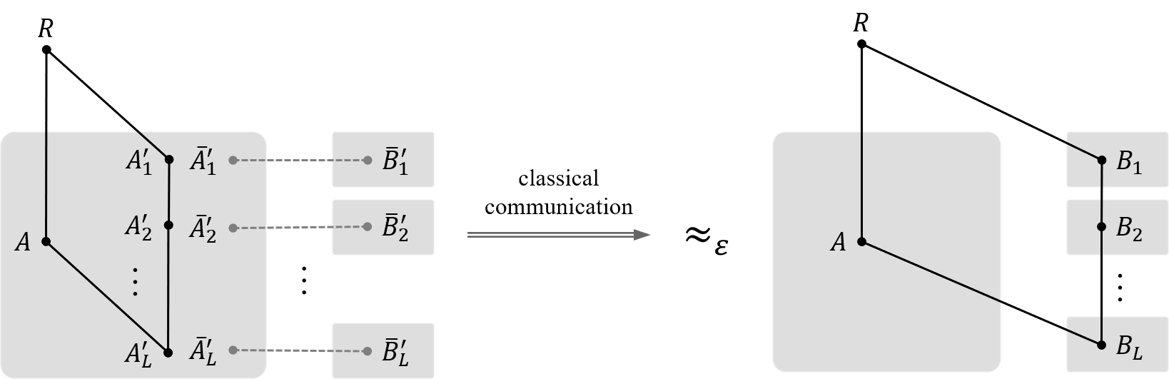
Figure 3. Depiction of $L$-party Quantum State Splitting protocol. Sender holds registers $A$, $A_{1}^{\prime}$, $\bar{A}_{1}^{\prime}$, $A_{2}^{\prime}$, $\bar{A}_{2}^{\prime}$, $\cdots$, $A_{L}^{\prime}$, $\bar{A}_{L}^{\prime}$, and pre-shares entanglement with each of the $L$ Receivers holding register $B_{\ell}^{\prime}$. $\ell\in[L]$; register $R$ represents an inaccessible Reference. Each grey-shaded region is allowed to perform local quantum operation at its holding registers, and (limited) noiseless classical communication from the sender to the $L$ receivers is permitted. After executing the protocol, we wish the systems $A_{1}^{\prime}$, $\cdots$, $A_{L}^{\prime}$ end up at each of the $\ell$-th receiver’s side (at the right part of the figure). Note that each gray-shaded region is only allowed to perform local quantum operation.

Definition ($L$-party Quantum State Splitting).

Let $\rho_{RAA_{1}^{\prime}A_{2}^{\prime}\ldots A_{L}^{\prime}}$ be a pure state as input of the protocol.

1. Quantum registers $A_{1}^{\prime}$, $A_{2}^{\prime}$, $\ldots$, $A_{L}^{\prime}$ and $A$ at Alice, $B_{1}\cong A_{1}^{\prime}$, $B_{2}\cong A_{2}^{\prime}$, $\ldots$, $B_{L}\cong A_{L}^{\prime}$ at $L$ Receivers, and $R$ at an inaccessible Reference.

2. A resource of entanglement, say $|\tau\rangle_{\bar{A}_{1}^{\prime}\bar{A}_{2}^{\prime}\ldots\bar{A}_{L}\bar{B}_{1}^{\prime}\bar{B}_{2}^{\prime}\ldots\bar{B}_{L}^{\prime}}$, shared between Sender (holding registers $\bar{A}_{1}^{\prime}\bar{A}_{2}^{\prime}\ldots\bar{A}_{L}^{\prime}$) and $L$ Receivers (each holding register $\bar{B}_{\ell}^{\prime}$, $\ell\in[L]$), and noiseless one-way classical communication from the sender to $L$ receivers are available.

3. The sender applies a local operation on her system and the shared entanglement to obtain $L$-tuple $\vec{r}:=(r_{1},r_{2},\ldots r_{L})$ bits of classical messages.

4. The sender sends the above message to each receiver, respectively, via noiseless one-way classical communication.

5. Upon receiving the messages, each receiver applies a local operation on his shared entanglement to obtain an overall state $\widehat{\rho}_{RAB_{1}B_{2}\ldots B_{L}}$.

A $(\vec{r},\varepsilon)$ $L$-party Quantum State Splitting protocol for $\rho_{RAA_{1}^{\prime}\ldots A_{L}^{\prime}}$ with entanglement
$|\tau\rangle_{\bar{A}_{1}^{\prime}\bar{A}_{2}^{\prime}\ldots\bar{A}_{L}\bar{B}_{1}^{\prime}\bar{B}_{2}^{\prime}\ldots\bar{B}_{L}^{\prime}}$ satisfies

$$\frac{1}{2}\left\|\widehat{\rho}_{RAB_{1}\ldots B_{L}}-\rho_{RAB_{1}\ldots B_{L}}\right\|_{1}\leq\varepsilon,$$ (4.1)

where $\rho_{RAB_{1}\ldots B_{L}}:=(\mathrm{id}_{A_{1}^{\prime}\ldots A_{L}^{\prime}\to B_{1}\ldots B_{L}}\otimes\mathrm{id}_{AR})\rho_{RAA_{1}^{\prime}A_{2}^{\prime}\ldots A_{L}^{\prime}}$.

For readability, we first show a special case of the bipartite Quantum State Splitting.

[$2$-party Quantum State Splitting] For any pure state $\rho_{AA_{1}^{\prime}A_{2}^{\prime}R}=|\rho\rangle\langle\rho|_{AA_{1}^{\prime}A_{2}^{\prime}R}$ , there exists a $(r_{1},r_{2},\varepsilon)$ $2$-party Quantum State Splitting protocol for $\rho_{RAA_{1}^{\prime}A_{2}^{\prime}}$ with entanglement $|\tau\rangle_{{A}_{1}^{\prime}{B}_{1}}$ and $|\tau\rangle_{{A}_{2}^{\prime}{B}_{2}}$ such that

$$\varepsilon \leq\sqrt{2\cdot 2^{-E_{r_{1}+r_{2}}\left(\rho_{A_{1}^{\prime}A_{2}^{\prime}R}\,\|\,\tau_{A_{1}^{\prime}}\otimes\tau_{A_{2}^{\prime}}\right)}+2^{-E_{r_{1}}\left(\rho_{A_{1}^{\prime}R}\,\|\,\tau_{A_{1}^{\prime}}\right)}+2^{-E_{r_{2}}\left(\rho_{A_{2}^{\prime}R}\,\|\,\tau_{A_{2}^{\prime}}\right)}},$$ (4.2)

where the error-exponent functions are defined in Eq. (2.23). Moreover, the error exponents are all positive if and only if,

$$\begin{cases}&r_{1}+r_{2}>I(\rho_{A_{1}^{\prime}A_{2}^{\prime}R}\,\|\,\tau_{A_{1}^{\prime}}\otimes\tau_{A_{2}^{\prime}}),\\ &r_{1}>I(\rho_{A_{1}^{\prime}R}\,\|\,\tau_{A_{1}^{\prime}}),\\ &r_{2}>I(\rho_{A_{2}^{\prime}R}\,\|\,\tau_{A_{2}^{\prime}}).\\ \end{cases}$$ (4.3)

Proof.

Unipartite Quantum State Splitting has been shown via unipartite convex splitting in Ref. [118] (see also [67]), Below we will demonstrate applying their approach with the newly established bipartite convex splitting (Theorem 3.1) to achieving a bipartite Quantum State Splitting protocol using $r_{1}$ and $r_{2}$ bits of classical communication with the desired error $\varepsilon$.

Let $M=2^{r_{1}}$ and $K=2^{r_{2}}$. We fix two states $\tau_{A_{1}^{\prime}}$ and $\tau_{A_{2}^{\prime}}$ that will be specify later. To begin the protocol, we let the sender (Alice) and the first receiver (Bob $1$) share $M$-copies of entanglement $\otimes_{m\in[M]}|\tau\rangle_{A_{1,m}^{\prime}B_{1,m}}$, and Alice and the second receiver (Bob $2$) share $K$-copies of entanglement $\otimes_{k\in[K]}|\tau\rangle_{A_{2,k}^{\prime}B_{2,k}}$, where for each $(m,k)\in[M]\times[K]$, Bob $1$ holds register $B_{1,m}\cong B_{1}$ that purifies Alice’s register $A_{1,m}^{\prime}\cong A_{1}^{\prime}$, and Bob $2$ holds register $B_{2,k}\cong B_{2}$ that purifies register Alice’s $A_{2,k}^{\prime}\cong A_{2}^{\prime}$. Hence, we start with the following pure state:

$$|\overline{\omega}\rangle:=|\rho\rangle_{AA_{1}^{\prime}A_{2}^{\prime}R}\otimes_{m\in[M]}|\tau\rangle_{A_{1,m}^{\prime}B_{1,m}}\otimes_{k\in[K]}|\tau\rangle_{A_{2,k}^{\prime}B_{2,k}}.$$ (4.4)

Suppose, hopefully, by the protocol, we end up with the following pure state:

$$\begin{split}|{\omega}\rangle&:=\frac{1}{\sqrt{MK}}\sum_{(m,k)\in[M]\times[K]}|m\rangle_{M}|k\rangle_{K}|\rho\rangle_{AB_{1,m}B_{2,k}R}|0\rangle_{A_{1,m}^{\prime}A_{2,k}^{\prime}}\otimes_{\bar{m}\in[M]\setminus\{m\}}|\tau\rangle_{A_{1,\bar{m}}^{\prime}B_{1,\bar{m}}}\otimes_{\bar{k}\in[K]\setminus\{k\}}|\tau\rangle_{A_{2,\bar{k}}^{\prime}B_{2,\bar{k}}},\end{split}$$ (4.5)

where Alice holds registers $M$, $K$, $A$, $A_{1,[M]}^{\prime}:=A_{1,1}^{\prime}\ldots A_{1,M}^{\prime}$ and $A_{2,[K]}^{\prime}:=A_{2,1}^{\prime}\ldots A_{2,K}^{\prime}$, and Bob 1 and Bob $2$ hold registers $B_{1,[M]}:=B_{1,1}\ldots B_{1,M}$ and $B_{2,[K]}:=B_{2,1}\cdots B_{2,K}$, respectively. Here, we shorthand for $A_{1,[M]}^{\prime}:=A_{1,1}^{\prime}\ldots A_{1,M}^{\prime}$ and $A_{2,[K]}^{\prime}:=A_{2,1}^{\prime}\ldots A_{2,K}^{\prime}$ (and similarly for $B_{1,[M]}$ and $B_{2,[K]}$) to ease the burden of notation. (We slightly abuse notation to use $M$ and $K$ denoting registers representing classical systems $[M]$ and $[K]$.) Alice measures on registers $M$ and $K$, and send on the outcome $m$ to Bob $1$ via $r_{1}$ bits of classical communication, and the outcome $k$ to Bob $2$ via $r_{2}$ bits of classical communication. Then, the two receivers can pick up registers $B_{1,m}$ and $B_{2,k}$, respectively, to end up with $|\rho\rangle_{AB_{1,m}B_{2,k}R}\cong|\rho\rangle_{AB_{1}B_{2}R}$, which is exactly the target state we aimed for the bipartite Quantum State Splitting protocol.

In what follows, we will show that there exists a local operation protocol at Alice such that we can approximate $|{\omega}\rangle$ in Eq. (4.5) within an error $\varepsilon$ no larger than the right-hand side of Eq. (4.2). Note that a reduced state of $|\overline{\omega}\rangle$ is

$$\overline{\omega}_{A_{1,[M]}^{\prime}A_{2,[K]}^{\prime}R} =\otimes_{m\in[M]}\tau_{A_{1,m}^{\prime}}\otimes_{k\in[K]}\tau_{A_{2,k}^{\prime}}\otimes\rho_{R}.$$ (4.6)

Then, the bipartite convex split lemma (Theorem 3.1) guarantees that $\overline{\omega}_{A_{1,[M]}^{\prime}A_{2,[K]}^{\prime}R}$ can be approximated by a state

$$\begin{split}\omega_{A_{1,[M]}^{\prime}A_{2,[K]}^{\prime}R}&:=\frac{1}{MK}\sum_{(m,k)\in[M]\times[K]}\rho_{A_{1,m}^{\prime}A_{2,k}^{\prime}R}\otimes_{\bar{m}\in[M]\setminus\{m\}}\tau_{A_{1,\bar{m}}^{\prime}}\otimes_{\bar{k}\in[K]\setminus\{k\}}\tau_{A_{2,\bar{k}}^{\prime}},\end{split}$$ (4.7)

within an error $\varepsilon^{\prime}$ (in terms of trace distance) no larger than the right-hand side of Eq. (3.30) (by substituting register $A$ by $A_{1}^{\prime}$, $B$ by $A_{2}^{\prime}$, and $E$ by $R$). Observe that $\omega_{A_{1,[M]}^{\prime}A_{2,[K]}^{\prime}R}$ is a reduced state of the desired pure state $|{\omega}\rangle$ given in Eq. (4.5). Hence, by Uhlmann’s theorem (Fact A), there exists an isometry $V$ acting on register $AA_{1}^{\prime}A_{2}^{\prime}A_{1,[M]}^{\prime}A_{2,[K]}^{\prime}$ to register $MKAA_{1,[M]}^{\prime}A_{2,[K]}^{\prime}$ such that $V|\overline{\omega}\rangle$ is $\sqrt{2\varepsilon^{\prime}}$-close (in trace distance) to $|\omega\rangle$. Moreover, since the isometry $V$ only acts on Alice’s registers, this constitutes the bipartite Quantum State Splitting protocol with error $\varepsilon$ no larger than $\sqrt{2\varepsilon^{\prime}}$. ∎

The above bipartite Quantum State Splitting is straightforwardly genearlized to any $L$-party case as follows. [$L$-party Quantum State Splitting] For any pure state $\rho_{AA_{1}^{\prime}A_{2}^{\prime}\ldots A_{L}^{\prime}R}=|\rho\rangle\langle\rho|_{AA_{1}^{\prime}A_{2}^{\prime}\ldots A_{L}^{\prime}R}$ , there exists a $(\vec{r},\varepsilon)$ $L$-party Quantum State Splitting protocol for $\rho_{RAA_{1}^{\prime}A_{2}^{\prime}\ldots A_{L}^{\prime}R}$ with entanglement $|\tau\rangle_{{A}_{\ell}^{\prime}{B}_{\ell}}$, $\ell\in[L]$ such that

$$\varepsilon \leq\sqrt{\sum\nolimits_{\varnothing\neq S\subseteq[L]}2^{|S|}\cdot 2^{-E_{r_{S}}\left(\rho_{A_{S}^{\prime}R}\,\|\,\tau_{A_{S}^{\prime}}\right)}},$$ (4.8)

where the error-exponent function is defined in Eq. (2.23), $r_{S}:=\sum_{\ell\in S}r_{\ell}$, $A_{S}^{\prime}$ denotes systems $A_{\ell}^{\prime}$ for all $\ell\in S$, and $\tau_{A_{S}^{\prime}}:=\otimes_{\ell\in S}\tau_{A_{\ell}^{\prime}}$. Moreover, the error exponents are all positive if and only if for all $\varnothing\neq S\subseteq[L]$ ,

$$r_{S}>I\left(\rho_{A_{S}^{\prime}R}\,\|\,\tau_{A_{S}^{\prime}}\right).$$ (4.9)

5. Entanglement-Assisted Quantum Broadcast Channel Simulation

Let $\mathscr{N}_{A\to B_{1}B_{2}\cdots B_{L}}$ be an $L$-receiver quantum broadcast channel, which is a completely positive and trace-preserving map from system $A$ to $L$ systems $B_{1}B_{2}\ldots B_{L}$.

Definition ($L$-party Quantum Broadcast Channel Simulation).

Let $\mathscr{N}_{A\to B_{1}B_{2}\cdots B_{L}}$ be a quantum broadcast channel as input of the simulation protocol.

1. Sender holds registers $A$. Each Receiver holds register $B_{1}$, $B_{2}$, $\ldots$, $B_{L}$, respectively.

2. Free resource of perfect entanglement is shared between Sender (holding registers $\bar{A}_{1}^{\prime}\bar{A}_{2}^{\prime}\ldots\bar{A}_{L}^{\prime}$) and each of the $L$ Receivers (holding register $\bar{B}_{\ell}^{\prime}$, $\ell\in[L]$).

3. Sender applies a local operation on her systems and sends an $L$-tuple $\vec{r}:=(r_{1},r_{2},\ldots r_{L})$ bits of classical information to each of the $L$ Receivers, respectively.

4. Upon receiving the message, each Receiver applies a local operation on his own system.

A $(\vec{r},\varepsilon)$ $L$-party Quantum Broadcast Channel Simulation protocol for $\mathscr{N}_{A\to B_{1}B_{2}\cdots B_{L}}$ satisfies

$$\frac{1}{2}\left\|\widehat{\mathscr{N}}_{A\to B_{1}B_{2}\cdots B_{L}}-\mathscr{N}_{A\to B_{1}B_{2}\cdots B_{L}}\right\|_{\diamond}\leq\varepsilon,$$ (5.1)

where $\widehat{\mathscr{N}}_{A\to B_{1}B_{2}\cdots B_{L}}$ is the effectively resulting linear transformation from Sender’s register $A$ to $L$ Receivers’ registers $B_{1}$, $\ldots$, $B_{L}$. The $L$-tuple $\vec{r}$ denotes the classical communication costs.

Definition (Capacity region for i.i.d. broadcast channel simulation).

The capacity region of simulating $\mathscr{N}_{A\to B_{1}B_{2}\cdots B_{L}}$, denoted as $\mathcal{C}(\mathscr{N}_{A\to B_{1}B_{2}\cdots B_{L}})$ is the closure of

$$\bigcup_{\varepsilon>0}\left\{\vec{r}\in\mathds{R}^{L}:\exists\,(n\vec{r},\varepsilon)\text{-$L$-party Quantum Broadcast Channel Simulation protocol for $\mathscr{N}^{\otimes n}$}\right\}.$$ (5.2)

[Non-asymptotic achievability for $2$-party Quantum Broadcast Channel Simulation] Let $\mathscr{N}_{A\to B_{1}B_{2}}$ be an $L$-receiver quantum broadcast channel. For any integer $n$, there exists an $(nr_{1},nr_{2},\varepsilon)$ Quantum Broadcast Channel Simulation protocol for $\mathscr{N}_{A\to B_{1}B_{2}}^{\otimes n}$ satisfying

$$\varepsilon \leq k_{n}\cdot\sqrt{2\cdot\delta_{1,2}+\delta_{1}+\delta_{2}},$$ (5.3)

$$\delta_{1,2} :=2^{-nE_{r_{1}+r_{2}}(\mathscr{N}_{A\to B_{1}B_{2}})},$$ (5.4)

$$\delta_{1} :=2^{-nE_{r_{1}}(\mathscr{N}_{A\to B_{1}})},$$ (5.5)

$$\delta_{2} :=2^{-nE_{r_{2}}(\mathscr{N}_{A\to B_{2}})},$$ (5.6)

where the error-exponent functions are defined in Eq. (2.25), and the polynomial prefactor is $k_{n}:=(n+1)^{\frac{5}{2}(|\mathsf{A}|^{2}-1)}$. Moreover, the three exponents $E_{r_{1}+r_{2}}(\mathscr{N}_{A\to B_{1}B_{2}})$ , $E_{r_{1}}(\mathscr{N}_{A\to B_{1}})$, $E_{r_{2}}(\mathscr{N}_{A\to B_{2}})$ are all positive if and only if

$$\begin{cases}&r_{1}+r_{2}>I(\mathscr{N}_{A\to B_{1}B_{2}}),\\ &r_{1}>I(\mathscr{N}_{A\to B_{1}}),\\ &r_{2}>I(\mathscr{N}_{A\to B_{2}}).\\ \end{cases}$$ (5.7)

[Capacity region for $2$-party Quantum Broadcast Channel Simulation] Let $\mathscr{N}_{A\to B_{1}B_{2}}$ be a quantum broadcast channel. The capacity region of simulating $\mathscr{N}_{A\to B_{1}B_{2}}$ is given by

$$\mathcal{C}(\mathscr{N}_{A\to B_{1}B_{2}}) =\left\{\vec{r}\in\mathds{R}^{2}:r_{1}+r_{2}\geq I(\mathscr{N}_{A\to B_{1}B_{2}}),\,r_{1}\geq I(\mathscr{N}_{A\to B_{1}}),\,r_{2}\geq I(\mathscr{N}_{A\to B_{2}})\right\}.$$ (5.8)

Remark .

Though our target is to simulate the broadcast channel $\mathscr{N}_{A\to B_{1}B_{2}}$, the established achievability given in Theorems 5 and 5 are actually stronger for the coherent feedback simulation of $\mathscr{N}_{A\to B_{1}B_{2}}$; namely, we are able to simulate the isometry $\mathscr{V}_{A\to B_{1}B_{2}E}$, where the complementary part $E$ is retained at Sender [119, 2].

Remark .

The minimax identity given in Proposition 2-iii shows that the error-exponent function of channel in Theorem 5 can be viewed as the error-exponent function for the channel output state induced by the worst-case input state. Namely, the error terms (i.e. $\delta_{1,2}$, $\delta_{1}$, and $\delta_{2}$ in Theorem 5) for channel simulation are dominated by the worst-case input states, respectively.

Proof of Theorem 5.

The achievability directly follows from the exponential decreases of error given in Theorem 5, and noting that $\lim_{n\in\infty}\frac{1}{n}\log k_{n}=0$.

For the converse, we first note that the the requirements on the separate rates $r_{1}$ and $r_{2}$ follow from the converse of the respective single-sender single-receiver reverse Shannon theorem [1, 2, 3]. That is, for an asymptotically vanishing error we need

$$r_{1}\geq I(\mathscr{N}_{A\to B_{1}}) r_{2}\geq I(\mathscr{N}_{A\to B_{2}})$$ and . (5.9)

For the rate sum constraint $r_{1}+r_{2}$ the argument is similar as in the classical case [43, Theorem 36] and a simple version for the first order asymptotics as needed here is as follows. The idea is to analyze the correlations between the purifying reference system $R$ and the respective receivers in terms of the multipartite mutual information. Any quantum broadcast simulation protocol applies an encoder on the sender’s side, uses classical communication at a rate $r_{i}$ from the sender to the $i$-th receiver’s side, and then applies local decoders on the receiver’s end. The multipartite mutual information is monotone under local operations at the receiver’s end (similarly as the mutual information) and increases at most by $nr_{i}$ by sending bits at a rate $r_{i}$ to the $i$-the receiver, as shown by the following dimension bound (cf. the textbook methods[120])

$$I(C_{1}X_{1}:C_{2}X_{2}:R)_{\sigma}\leq I(C_{1}:C_{2}:R)_{\sigma}+\log|\mathsf{X}_{1}|+\log|\mathsf{X}_{2}|$$ (5.10)

for any classical-quantum state $\sigma_{X_{1}X_{2}C_{1}C_{2}}$, classical on systems $X_{1}X_{2}$. However, at the end of any $\varepsilon$-good protocol (Definition 5) for a purified i.i.d. input state $(\psi^{\rho}_{AR})^{\otimes n}$, the output state on the relevant systems has to be $\varepsilon$-close in variational distance to $\left[(\mathscr{N}_{A\to B_{1}B_{2}}\otimes\mathcal{I}_{R})(\psi^{\rho}_{AR})\right]^{\otimes n}$. As the continuity of the multipartite mutual information is inherited from the continuity of the von Neumann entropy (see, e.g., [121] for tight estimates), we need at the end of the protocol that the multipartite mutual information on the relevant systems obeys

$$n\cdot I(B_{1}:B_{2}:R)_{(\mathscr{N}\otimes\mathcal{I})(\psi^{\rho})}\leq nr_{1}+nr_{2}+O(n\varepsilon\log|\mathsf{B}_{1}||\mathsf{B}_{2}|)\,,$$ (5.11)

where we also employed that the multipartite mutual information is additive on tensor product states. Since this has to hold for any i.i.d. input states $\rho_{A}^{\otimes n}$, the claim follows from taking the limit $\varepsilon\to 0$ for asymptotically perfect protocols. ∎

[Error exponent] Let $\mathscr{N}_{A\to B_{1}B_{2}}$ be a quantum broadcast channel. There exists a sequence of $(n\vec{r},\varepsilon_{n})$ Quantum Broadcast Channel Simulation protocol for $\mathscr{N}_{A\to B_{1}B_{2}}^{\otimes n}$ satisfying achievable error exponent bound:

$$\liminf_{n\to\infty}-\frac{1}{n}\log\varepsilon_{n}\geq\frac{1}{2}\min\left\{E_{r_{1}+r_{2}}(\mathscr{N}_{A\to B_{1}B_{2}}),E_{r_{1}}(\mathscr{N}_{A\to B_{1}}),E_{r_{2}}(\mathscr{N}_{A\to B_{2}})\right\}.$$ (5.12)

Moreover, the overall error exponent in the lower bound is positive if and only if $\vec{r}$ is in the interior of the capacity region $\mathcal{C}(\mathscr{N})$ given in Eq. (5.8).

Remark .

The optimal error exponent (under channel purified distance) was established for point-to-point quantum channel simulation [46]. Even for the special case of point-to-point quantum channel simulation, it is not clear whether the error exponent given in Proposition 5 or the result in [46] will give a better error exponent under diamond norm due to the fundamental different expressions of the error-exponent functions.

Our intention in this paper, however, is not to derive the optimal error exponent, but to devise a machinery for analyzing one-shot quantum broadcast channel simulation and the corresponding capacity region.

The overall error exponent for Quantum Broadcast Channel Simulation is positive if and only if the classical communication cost $\vec{r}$ is in the interior of the capacity region $\mathcal{C}(\mathscr{N})$ as shown in Theorem 5 and Proposition 5. One may wonder if the broadcast channel simulation is still achievable as $\vec{r}$ asymptotically converges to the boundary $\mathcal{C}(\mathscr{N})$? Note that in this scenario the overall error exponent will vanish asymptotically. In the following Proposition 5, we show that the broadcast channel simulation is still achievable once $\vec{r}$ converges to the boundary $\mathcal{C}(\mathscr{N})$ of speed $\Theta(n^{-t})$ for some $t\in(0,\nicefrac{{1}}{{2}})$. We call such $\Theta(n^{-t})$ a strictly moderate sequence [122, 123, 23, 45] and such a study as a moderate deviation analysis (compared to the large deviation analysis given in Theorem 5 and Proposition 5, in which $\vec{r}$ is bounded away from the boundary of $\mathcal{C}(\mathscr{N})$).

[Achievability for moderate deviation analysis] Let $\mathscr{N}_{A\to B_{1}B_{2}}$ be a quantum broadcast channel on finite-dimensional Hilbert spaces. For any sequence $\vec{r}_{n}:=(r_{1,n},r_{2,n})\in\mathcal{C}(\mathscr{N}_{A\to B_{1}B_{2}})$ satisfying

$$a_{n}:=\min\left\{\frac{r_{1,n}-I(\mathscr{N}_{A\to B_{1}})}{\sqrt{V(\mathscr{N}_{A\to B_{1}})}},\frac{r_{2,n}-I(\mathscr{N}_{A\to B_{2}})}{\sqrt{V(\mathscr{N}_{A\to B_{1}})}}\frac{r_{1,n}+r_{2,n}-I(\mathscr{N}_{A\to B_{1}B_{2}})}{\sqrt{V(\mathscr{N}_{A\to B_{1}B_{2}})}}\right\}=\Theta(n^{-t})$$ (5.13)

for some $t\in(0,\nicefrac{{1}}{{2}})$, then there exists a sequence of $(n\vec{r}_{n},\varepsilon_{n})$ Quantum Broadcast Channel Simulation protocols for $\mathscr{N}_{A\to B_{1}B_{2}}^{\otimes n}$ such that

$$\liminf_{n\to\infty}-\frac{1}{na_{n}^{2}}\log\varepsilon_{n}\geq\frac{1}{4}.$$ (5.14)

Remark .

For the special case of point-to-point quantum channel simulation, Proposition 5 translates to the following scenario: given $\varepsilon_{n}=2^{-na_{n}^{2}}$, then there exists a sequence of $(nr_{n},\varepsilon_{n})$-quantum channel simulation protocols for $\mathscr{N}_{A\to B}^{\otimes n}$ such that $r_{n}\leq I(\mathscr{N})+2\sqrt{V(\mathscr{N})}\cdot a_{n}$. Such an achievable rate for classical communication cost coincides with the result given in [45] (under channel purified distance). We expect that the best achievable moderate deviation expansion of the classical communication cost under diamond norm is $I(\mathscr{N})+\sqrt{2V(\mathscr{N})}\cdot a_{n}$, which is left as a future work.

The proof of Proposition 5 follows from the achievability given in Theorem 5, the properties of error-exponent function (Proposition 2), and the standard moderate deviation analysis given in [111, 86, 23].

Proof.

Let us first consider the unipartite case, i.e. $\mathscr{N}_{A\to B}$ provided that $V(\mathscr{N}_{A\to B})>0$. Let

$$r_{n} :=I(\mathscr{N})+a_{n},$$ (5.15)

where $(a_{n})_{n\in\mathds{N}}$ is any positive sequence satisfying $a_{n}=\Theta(n^{-t})$ for some $t\in(0,\nicefrac{{1}}{{2}})$. We recall Proposition 2-iv:

$$\liminf_{n\to\infty}\frac{E_{r_{n}}(\mathscr{N})}{a_{n}^{2}} \geq\frac{1}{2V(\mathscr{N})}.$$ (5.16)

Then by Theorem 5 (with $L=1$), we estimate the error probability for simulating $\mathscr{N}_{A\to B}^{\otimes n}$ using rate $nr_{n}$ as

$$\liminf_{n\to\infty}-\frac{1}{na_{n}^{2}}\log\varepsilon(\mathscr{N}_{A\to B}^{\otimes n}) \geq\liminf_{n\to\infty}-\frac{1}{na_{n}^{2}}\log\left\{k_{n}\sqrt{2^{-E_{nr_{n}}(\mathscr{N}^{\otimes n})}}\right\}$$ (5.17)

$$=\liminf_{n\to\infty}\left\{\frac{E_{nr_{n}}(\mathscr{N}^{\otimes n})}{2na_{n}^{2}}-\log\frac{k_{n}}{na_{n}^{2}}\right\}$$ (5.18)

$$=\liminf_{n\to\infty}\left\{\frac{E_{r_{n}}(\mathscr{N})}{2a_{n}^{2}}-\log\frac{k_{n}}{n^{1-2t}}\right\}$$ (5.19)

$$\geq\frac{1}{4V(\mathscr{N}_{A\to B})},$$ (5.20)

where the last line holds for any polynomial pre-factor $k_{n}$ for any $t\in(0,\nicefrac{{1}}{{2}})$. This leads to our assertion of the moderate deviation achievability for simulating point-to-point channel $\mathscr{N}_{A\to B}$ via re-scaling $r_{n}=I(\mathscr{N})+a_{n}$ by $r_{n}=I(\mathscr{N})+\sqrt{V(\mathscr{N})}\cdot a_{n}$.

Similar reasoning straightforwardly applies to the multipartite case, i.e. for any non-empty subset $S\subseteq[L]$ (with fixed $L\in\mathds{N}$), we have

$$\liminf_{n\to\infty}\frac{E_{r_{n}}(\mathscr{N}_{A\to B_{S}})}{a_{n}^{2}} \geq\frac{1}{2V(\mathscr{N}_{A\to B_{S}})},$$ (5.21)

and thus

$$\liminf_{n\to\infty}-\frac{1}{na_{n}^{2}}\log\varepsilon(\mathscr{N}_{A\to B_{S}}^{\otimes n}) \geq\frac{1}{4V(\mathscr{N}_{A\to B_{S}})}.$$ (5.22)

Combined with Theorem 5. The overall asymptotic error decay will be dominated by the worst channel output subset $S$. This concludes the proof. ∎

We now present the proof of bipartite quantum broadcast channel simulation.

Proof of Theorem 5.

Before diving into the proof, let us first elaborate on the proof structure. Our main technique relies on the multipartite Quantum State Splitting established in Section 4 and the Post-Selection Technique [70]. Note that the idea of unipartite Quantum State Splitting and the Post-Selection Technique have been used to prove point-to-point quantum channel simulation [3]. Unlike [3] working with the smooth entropy formalism, we will demonstrate how the Post-Selection Technique can work with Rényi information measures by employing certain properties shown in Lemmas 2 and 2.

We start with the de Finetti type input state: $\zeta_{AR}^{n}=\int\psi_{AR}^{\otimes n}\,\mathrm{d}(\psi_{AR})$, where $\psi_{AR}\in\mathcal{S}(\mathsf{A}\otimes\mathsf{R})$ is a pure state, and the integration is with respect to the Haar measure on the unitary group acting on $\mathsf{A}\otimes\mathsf{R}$. Moreover, we denote by $\zeta_{ARR^{\prime}}^{n}$ a purification of $\zeta_{AR}^{n}$. Let $\mathscr{U}_{A\to B_{1}B_{2}E}$ be a Stinespring dilation of the broadcast channel $\mathscr{N}_{A\to B_{1}B_{2}}$. Then, Sender first simulate a local isometry $\mathscr{N}_{A\to B_{1}B_{2}}$ at her side to obtain the state

$$\zeta_{B_{1}B_{2}ERR^{\prime}}^{n}:=\left(\mathscr{U}_{A\to B_{1}B_{2}E}^{\otimes n}\otimes\mathrm{id}_{RR^{\prime}}\right)\zeta_{ARR^{\prime}}^{n}.$$ (5.23)

Next, we apply the $2$-party Quantum State Splitting protocol (Theorem 3) with registers $A\leftarrow E$, $A_{1}^{\prime}\leftarrow B_{1}$, $A_{2}^{\prime}\leftarrow B_{2}$, and $R\leftarrow RR^{\prime}$, to send the $B_{1}$-part to Receiver $1$ via $nr_{1}$ bits of classical communication and send the $B_{2}$-part to Receiver $2$ via $nr_{2}$ bits of classical communication. The pre-shared entanglement used in the protocol is many copies of $|\zeta^{n}\rangle_{B_{1}\bar{B}_{1}}$ and $|\zeta^{n}\rangle_{B_{2}\bar{B}_{2}}$, where the first Receiver holds register $\bar{B}_{1}^{n}$ and the second Receiver holds register $\bar{B}_{2}^{n}$. The above procedure is embodied by a simulated isometry $\widehat{\mathscr{U}}_{A\to B_{1}B_{2}E}^{n}$ acting on the state $\zeta_{ARR^{\prime}}^{n}$. Then, the resulting error, denoted by $\varepsilon^{\prime}(\zeta^{n})$, is

$$\frac{1}{2}\left\|\left(\widehat{\mathscr{U}}_{A\to B_{1}B_{2}E}^{n}-\mathscr{U}_{A\to B_{1}B_{2}E}^{\otimes n}\right)(\zeta_{ARR^{\prime}}^{n})\right\|_{1} \leq\varepsilon^{\prime}(\zeta^{n}),$$ (5.24)

$$\varepsilon^{\prime}(\zeta^{n}) :=\sqrt{2\cdot\delta_{1,2}^{\prime}(\zeta^{n})+\delta_{1}^{\prime}(\zeta^{n})+\delta_{2}^{\prime}(\zeta^{n})},$$ (5.25)

$$\delta_{1,2}^{\prime}(\zeta^{n}) :=2^{-E_{nr_{1}+nr_{2}}(B_{1}:B_{2}:RR^{\prime})_{(\mathscr{N}^{\otimes n}\otimes\mathrm{id})(\zeta^{n})}},$$ (5.26)

$$\delta_{1}^{\prime}(\zeta^{n}) :=2^{-E_{nr_{1}}(B_{1}:RR^{\prime})_{(\mathscr{N}^{\otimes n}\otimes\mathrm{id})(\zeta^{n})}},$$ (5.27)

$$\delta_{2}^{\prime}(\zeta^{n}) :=2^{-E_{nr_{2}}(B_{2}:RR^{\prime})_{(\mathscr{N}^{\otimes n}\otimes\mathrm{id})(\zeta^{n})}},$$ (5.28)

where the error-exponent function is defined in Eq. (2.24). Moreover, by tracing out the system $E^{n}$ and the monotonicity of trace distance [124], we obtain the bound:

$$\frac{1}{2}\left\|\left(\widehat{\mathscr{N}}_{A\to B_{1}B_{2}}^{n}-\mathscr{N}_{A\to B_{1}B_{2}}^{\otimes n}\right)(\zeta_{ARR^{\prime}}^{n})\right\|_{1}\leq\varepsilon^{\prime}(\zeta^{n}).$$ (5.29)

Here, the channel $\widehat{\mathscr{N}}_{A\to B_{1}B_{2}}^{n}$ is the effectively simulated proximity to our target $\mathscr{N}_{A\to B_{1}B_{2}}^{\otimes n}$.

By using the Post-Selection Technique (Proposition B), this guarantees that

$$\begin{split}\frac{1}{2}\left\|\widehat{\mathscr{N}}_{A\to B_{1}B_{2}}^{n}-\mathscr{N}_{A\to B_{1}B_{2}}^{\otimes n}\right\|_{\diamond}\leq(n+1)^{|\mathsf{A}|^{2}-1}\varepsilon^{\prime}(\zeta^{n}).\end{split}$$ (5.30)

It remains to remove the auxiliary system $R^{\prime}$ and to upper bound the error $\varepsilon^{\prime}(\zeta^{n})$ with the one dominated by the worst-case state $\psi_{AR}^{\otimes n}$ in the mixture of the de Finetti type state $\zeta_{AR}^{n}$.

Note that we can assume $|\mathsf{R}^{\prime}|\leq(n+1)^{|\mathsf{A}|^{2}-1}$ by Fact B. Further, Lemma 2 shows that, for each $\alpha>0$,

$$I_{\alpha}(B_{1}:B_{2}:RR^{\prime})_{(\mathscr{N}^{\otimes n}\otimes\mathrm{id})(\zeta^{n})}\leq I_{\alpha}(B_{1}:B_{2}:R)_{(\mathscr{N}^{\otimes n}\otimes\mathrm{id})(\zeta^{n})}+\frac{2\alpha}{\alpha-1}\log\left[(n+1)^{|\mathsf{A}|^{2}-1}\right],$$ (5.31)

which by the definition of the error-exponent function in Eq. (2.24), in turn, implies that

$$E_{nr_{1}+nr_{2}}(B_{1}:B_{2}:RR^{\prime})_{(\mathscr{N}^{\otimes n}\otimes\mathrm{id})(\zeta^{n})}\geq E_{nr_{1}+nr_{2}}(B_{1}:B_{2}:R)_{(\mathscr{N}^{\otimes n}\otimes\mathrm{id})(\zeta^{n})}-2\log\left[(n+1)^{|\mathsf{A}|^{2}-1}\right];$$ (5.32)

likewise for $E_{nr_{1}}(B_{1}:RR^{\prime})_{(\mathscr{N}^{\otimes n}\otimes\mathrm{id})(\zeta^{n})}$ and $E_{nr_{2}}(B_{2}:RR^{\prime})_{(\mathscr{N}^{\otimes n}\otimes\mathrm{id})(\zeta^{n})}$.

Using Carathéodory’s type theorem (Fact B), we can write

$$\zeta_{AR}^{n}=\sum\nolimits_{i\in\mathcal{I}}p_{i}(\psi_{AR}^{i})^{\otimes n}$$ (5.33)

for some pure state $\psi_{AR}^{i}$, finite set $\mathcal{I}$ with $|\mathcal{I}|=(n+1)^{2|\mathsf{A}||\mathsf{R}|-2}$, and probability distribution $\{p_{i}\}_{i\in\mathcal{I}}$. Then, Lemma 2 with $L=2$ and the additivity of Rényi information (Proposition 2-b) show that

$$I_{\alpha}(B_{1}:B_{2}:R)_{(\mathscr{N}^{\otimes n}\otimes\mathrm{id})(\sum_{i}p_{i}(\psi^{i})^{\otimes n})} \leq\sum\nolimits_{i\in\mathcal{I}}p_{i}I_{\alpha}(B_{1}:B_{2}:R)_{(\mathscr{N}^{\otimes n}\otimes\mathrm{id})((\psi^{i})^{\otimes n})}+2\log\left[(n+1)^{2|\mathsf{A}||\mathsf{R}|-2}\right]$$ (5.34)

$$=\sum\nolimits_{i\in\mathcal{I}}p_{i}nI_{\alpha}(B_{1}:B_{2}:R)_{(\mathscr{N}\otimes\mathrm{id})(\psi^{i})}+2\log\left[(n+1)^{|\mathsf{A}||\mathsf{R}|-2}\right]$$ (5.35)

$$\leq\max_{i\in\mathcal{I}}nI_{\alpha}(B_{1}:B_{2}:R)_{(\mathscr{N}\otimes\mathrm{id})(\psi^{i})}+2\log\left[(n+1)^{2|\mathsf{A}||\mathsf{R}|-2}\right]$$ (5.36)

$$\leq nI_{\alpha}(\mathscr{N}_{A\to B_{1}B_{2}})+2\log\left[(n+1)^{2|\mathsf{A}||\mathsf{R}|-2}\right].$$ (5.37)

This then implies that

$$E_{nr_{1}+nr_{2}}(B_{1}:B_{2}:R)_{(\mathscr{N}^{\otimes n}\otimes\mathrm{id})(\zeta^{n})}\geq nE_{r_{1}+r_{2}}(\mathscr{N}_{A\to B_{1}B_{2}})-\log\left[(n+1)^{2|\mathsf{A}||\mathsf{R}|-2}\right].$$ (5.38)

Similar bounds hold for $E_{nr_{1}}(B_{1}:R)_{(\mathscr{N}^{\otimes n}\otimes\mathrm{id})(\zeta^{n})}$ and $E_{nr_{2}}(B_{2}:R)_{(\mathscr{N}^{\otimes n}\otimes\mathrm{id})(\zeta^{n})}$ as well.

Lastly, combining the prefactors incurred in Eq. (5.30), Eq. (5.32), and Eq. (5.38), we conclude the proof from Eq. (5.25) with the overall polynomial prefactor:

$$(n+1)^{\frac{|\mathsf{A}|^{2}-1}{2}}(n+1)^{|\mathsf{A}|^{2}-1}(n+1)^{{|\mathsf{A}||\mathsf{R}|-1}}\leq(n+1)^{\frac{5}{2}(|\mathsf{A}|^{2}-1)}=:k_{n}.$$ (5.39)

∎

The scenario of simulation arbitrary $L$-party quantum broadcast channel follows the same proof as in the bipartite case (Theorem 5) and the multipartite Quantum State Splitting established in Theorem 3. [Non-asymptotic achievability for $L$-party Quantum Broadcast Channel Simulation] Let $\mathscr{N}_{A\to B_{1}B_{2}\ldots B_{L}}$ be an $L$-receiver quantum broadcast channel. For any integer $n$, there exists an $(n\vec{r},\varepsilon)$ Quantum Broadcast Channel Simulation protocol for $\mathscr{N}_{A\to B_{1}B_{2}\ldots B_{L}}^{\otimes n}$ satisfying

$$\varepsilon \leq k_{n}\cdot\sqrt{\sum\nolimits_{\varnothing\neq S\subseteq[L]}2^{|S|}\cdot 2^{-nE_{r_{S}}(\mathscr{N}_{A\to B_{S}})}},$$ (5.40)

where the error-exponent functions are defined in Eq. (2.25), the polynomial prefactor is $k_{n}:=(n+1)^{\frac{3+L}{2}(|\mathsf{A}|^{2}-1)}$, $r_{S}:=\sum_{\ell\in S}r_{\ell}$, and $B_{S}$ denotes systems $B_{\ell}$ for all $\ell\in S$.

[Capacity region for $L$-party Quantum Broadcast Channels Simulation] Let $\mathscr{N}_{A\to B_{1}B_{2}\ldots B_{L}}$ be an $L$-receiver quantum broadcast channel. The capacity region of simulating $\mathscr{N}_{A\to B_{1}B_{2}\ldots B_{L}}$ is given by

$$\mathcal{C}(\mathscr{N}_{A\to B_{1}\ldots B_{L}})=\left\{\vec{r}\in\mathds{R}^{L}:\sum\nolimits_{\ell\in S}r_{\ell}\geq I(\mathscr{N}_{A\to B_{S}}),\forall S\subseteq[L]\right\},$$ (5.41)

where $B_{S}$ denotes systems $B_{\ell}$ for all $\ell\in S$. Moreover, the lower bound to the error exponent and the achievability of moderate deviations as stated in Propositions 5 and 5 also immediately hold for $L$-receiver broadcast channel simulation.

Appendix A Technical Lemmas

Fact (Uhlmann’s theorem [125], [126], [42, Lemma 2.2]).

Let $\psi_{AB}=|\psi\rangle\langle\psi|_{AB}$ and $\varphi_{AC}=|\varphi\rangle\langle\varphi|_{AC}$ be two pure quantum states. Then, there exists an isometry $\mathscr{V}_{B\to C}$ satisfying

$$\frac{1}{2}\|\psi_{A}-\varphi_{A}\|_{1}\leq\varepsilon\Rightarrow\frac{1}{2}\|\mathscr{V}_{B\to C}(\psi_{AB})-\varphi_{AC}\|_{1}=\mathrm{P}(\mathscr{V}_{B\to C}(\psi_{AB}),\varphi_{AC})\leq\sqrt{2\varepsilon-\varepsilon^{2}}\leq\sqrt{2\varepsilon}.$$ (A.1)

Lemma 2 (Dimension bound).

For any states $\rho_{ABC}\in\mathcal{S}(\mathsf{A}\otimes\mathsf{B}\otimes\mathsf{C})$, $\tau_{A}\in\mathcal{S}(\mathsf{A})$, and $\alpha>0$, we have

$$I_{\alpha}\left(\rho_{ABC}\,\|\,\tau_{A}\right)\leq I_{\alpha}\left(\rho_{AB}\,\|\,\tau_{A}\right)+\frac{2\alpha}{\alpha-1}\log|\mathsf{C}|.$$ (A.2)

Proof.

For every $\varepsilon>0$, let $\sigma_{B}\in\mathcal{S}(\mathsf{B})$ be a density operator satisfying

$$D_{\alpha}(\rho_{AB}\,\|\,\tau_{A}\otimes\sigma_{B})\leq I_{\alpha}\left(\rho_{AB}\,\|\,\tau_{A}\right)+\varepsilon,$$ (A.3)

and denote by $\tilde{\sigma}_{BC}:=\sigma_{B}\otimes\frac{\mathds{1}_{C}}{|\mathsf{C}|}$ for short. Note that $\rho_{ABC}\leq|\mathsf{C}|\cdot\rho_{AB}\otimes\mathds{1}_{C}$, which implies

$$\frac{1}{|\mathsf{C}|^{2}}\rho_{ABC}\leq\rho_{AB}\otimes\frac{\mathds{1}_{C}}{|\mathsf{C}|}.$$ (A.4)

Then,

$$\frac{1}{|\mathsf{C}|^{2}}\left(\tau_{A}\otimes\tilde{\sigma}_{BC}\right)^{\frac{1-\alpha}{2\alpha}}\rho_{ABC}\left(\tau_{A}\otimes\tilde{\sigma}_{BC}\right)^{\frac{1-\alpha}{2\alpha}}\leq\left(\tau_{A}\otimes\tilde{\sigma}_{BC}\right)^{\frac{1-\alpha}{2\alpha}}\rho_{AB}\otimes\frac{\mathds{1}_{C}}{|\mathsf{C}|}\left(\tau_{A}\otimes\tilde{\sigma}_{BC}\right)^{\frac{1-\alpha}{2\alpha}}.$$ (A.5)

This implies, for all $\alpha>0$,

$$\frac{1}{|\mathsf{C}|^{2}}\left\|\left(\tau_{A}\otimes\tilde{\sigma}_{BC}\right)^{\frac{1-\alpha}{2\alpha}}\rho_{ABC}\left(\tau_{A}\otimes\tilde{\sigma}_{BC}\right)^{\frac{1-\alpha}{2\alpha}}\right\|_{\alpha}\leq\left\|\left(\tau_{A}\otimes\tilde{\sigma}_{BC}\right)^{\frac{1-\alpha}{2\alpha}}\rho_{AB}\otimes\frac{\mathds{1}_{C}}{|\mathsf{C}|}\left(\tau_{A}\otimes\tilde{\sigma}_{BC}\right)^{\frac{1-\alpha}{2\alpha}}\right\|_{\alpha}.$$ (A.6)

By invoking the definition of the sandwiched Rényi divergence $D_{\alpha}(\rho\,\|\,\sigma):=\frac{\alpha}{\alpha-1}\log\left\|\sigma^{\frac{1-\alpha}{2\alpha}}\rho\sigma^{\frac{1-\alpha}{2\alpha}}\right\|_{\alpha}$, we have

$$D_{\alpha}\left(\rho_{ABC}\,\|\,\tau_{A}\otimes\tilde{\sigma}_{BC}\right)-\frac{2\alpha}{\alpha-1}\log|\mathsf{C}| \leq D_{\alpha}\left(\left.\rho_{AB}\otimes\frac{\mathds{1}_{C}}{|\mathsf{C}|}\,\right\|\,\tau_{A}\otimes\tilde{\sigma}_{BC}\right)$$ (A.7)

$$=D_{\alpha}\left(\rho_{AB}\,\|\,\tau_{A}\otimes{\sigma}_{B}\right)$$ (A.8)

$$\leq I_{\alpha}\left(\rho_{AB}\,\|\,\tau_{A}\right)+\varepsilon,$$ (A.9)

where we have used the fact that the sandwiched Rényi divergence remains identical by appending a state.

Lastly, by definition, noting that

$$D_{\alpha}\left(\rho_{ABC}\,\|\,\tau_{A}\otimes\tilde{\sigma}_{BC}\right)\geq I_{\alpha}\left(\rho_{ABC}\,\|\,\tau_{A}\right),$$ (A.10)

and letting $\varepsilon\to 0$ conclude the proof. ∎

Lemma 2 (Convexity).

Let $L$ be any integer and $\mathcal{I}$ be any finite set. Let $\rho_{A_{1}A_{2}\ldots A_{L}E}:=\sum_{i\in\mathcal{I}}p_{i}\rho_{A_{1}A_{2}\ldots A_{L}E}^{i}$ and $\tau_{A_{\ell}}=\sum_{i\in\mathcal{I}}p_{i}\tau_{A_{\ell}}^{i}$, $\ell\in[L]$ be statistical mixtures of states for any $p_{i}>0$, $\sum_{i\in\mathcal{I}}p_{i}=1$. Then, the following holds for every $\alpha\geq\nicefrac{{1}}{{2}}$,

$$\begin{split}I_{\alpha}(\rho_{A_{1}\ldots A_{L}E}\,\|\otimes_{\ell\in[L]}\tau_{A_{\ell}})&\leq\sum\nolimits_{i\in\mathcal{I}}p_{i}I_{\alpha}\left(\rho_{A_{1}\ldots A_{L}E}^{i}\,\|\otimes_{\ell\in[L]}\tau_{A_{\ell}}^{i}\right)+L\cdot H(\{p_{i}\}_{i\in\mathcal{I}})\\ &\leq\sum\nolimits_{i\in\mathcal{I}}p_{i}I_{\alpha}\left(\rho_{A_{1}\ldots A_{L}E}^{i}\,\|\otimes_{\ell\in[L]}\tau_{A_{\ell}}^{i}\right)+L\log|\mathcal{I}|.\end{split}$$ (A.11)

Here, $H(\{p_{i}\}_{i\in\mathcal{I}}):=-\sum_{i\in\mathcal{I}}p_{i}\log p_{i}$ denotes the Shannon entropy.

Proof.

Below, the subscript $\ell$ runs over all $[L]$ and the subscript $i$ runs over all $\mathcal{I}$ if we do not specify it. For each $i\in\mathcal{I}$ and every $\varepsilon>0$, we let $\sigma_{E}^{i}\in\mathcal{S}(\mathsf{E})$ to be a state satisfying

$$D_{\alpha}\left(\rho_{A_{1}\ldots A_{L}E}^{i}\,\|\otimes_{\ell}\tau_{A_{\ell}}^{i}\otimes\sigma_{E}^{i}\right)\leq I_{\alpha}\left(\rho_{A_{1}\ldots A_{L}E}^{i}\,\|\,\otimes_{\ell}\tau_{A_{\ell}}^{i}\right)+\varepsilon.$$ (A.12)

Then, by the definition of the sandwiched Rényi divergence, we have

$$\sum\nolimits_{i}p_{i}D_{\alpha}\left(\rho_{A_{1}\ldots A_{L}E}^{i}\,\|\otimes_{\ell}\tau_{A_{\ell}}^{i}\otimes\sigma_{E}^{i}\right)-L\cdot p_{i}\log p_{i}$$ (A.13)

$$=\sum\nolimits_{i}p_{i}D_{\alpha}\left(\rho_{A_{1}\ldots A_{L}E}^{i}\,\|\,p_{i}\tau_{A_{1}}^{i}\otimes\cdots\otimes p_{i}\tau_{A_{L}}^{i}\otimes\sigma_{E}^{i}\right)$$ (A.14)

$$\overset{\textnormal{(a)}}{\geq}D_{\alpha}\left(\sum\nolimits_{i}p_{i}\rho_{A_{1}\ldots A_{L}E}^{i}\,\|\sum\nolimits_{i}p_{i}\tau_{A_{1}}^{i}\otimes\cdots\otimes p_{i}\tau_{A_{L}}^{i}\otimes p_{i}\sigma_{E}^{i}\right)$$ (A.15)

$$\overset{\textnormal{(b)}}{\geq}D_{\alpha}\left(\sum\nolimits_{i}p_{i}\rho_{A_{1}\ldots A_{L}E}^{i}\,\|\sum\nolimits_{i_{1}}p_{i_{1}}\tau_{A_{1}}^{i_{1}}\otimes\cdots\otimes\sum\nolimits_{i_{L}}p_{i_{L}}\tau_{A_{L}}^{i_{1}}\otimes\sum\nolimits_{i}p_{i}\sigma_{E}^{i}\right)$$ (A.16)

$$=D_{\alpha}\left(\rho_{A_{1}\ldots A_{L}E}\,\|\tau_{A_{1}}\otimes\cdots\otimes\tau_{A_{L}}\otimes\sum\nolimits_{i}p_{i}\sigma_{E}^{i}\right)$$ (A.17)

$$\geq I_{\alpha}(\rho_{A_{1}\ldots A_{L}E}\,\|\otimes_{\ell\in[L]}\tau_{A_{\ell}}),$$ (A.18)

where (a) follows from the convexity of the sandwiched Rényi divergence [77, 78, 127, 128], [129, Theorem 3.16], and (b) follows from the monotonically non-increasing map $\sigma\mapsto D_{\alpha}(\rho\,\|\,\sigma)$ [77, Proposition 4], [129, Lemma 3.24], and for each $\ell\in[L]$, $p_{i}\tau_{A_{\ell}}^{i}\leq\sum\nolimits_{i_{\ell}\in[L]}p_{i_{\ell}}\tau_{A_{\ell}}^{{i}_{\ell}}$. By letting $\varepsilon\to 0$, we conclude the proof. ∎

Proposition 2 (Properties of error-exponent function).

For any multipartite state $\rho_{A_{1}A_{2}\ldots A_{L}B}$ and any quantum broadcast channel $\mathscr{N}_{A\to B_{1}B_{2}\ldots B_{L}}$, the error-exponent function satisfies the following properties.

1. (Positivity) For any $r>0$,

   $$E_{r}(\rho_{A_{1}A_{2}\ldots A_{L}B}\,\|\otimes_{\ell\in[L]}\tau_{A_{\ell}})>0 \Longleftrightarrow r>I(\rho_{A_{1}A_{2}\ldots A_{L}B}\,\|\otimes_{\ell\in[L]}\tau_{A_{\ell}});$$ (A.19)

   $$E_{r}(\mathscr{N}_{A\to B_{1}B_{2}\ldots B_{L}})>0 \Longleftrightarrow r>I(\mathscr{N}_{A\to B_{1}B_{2}\ldots B_{L}}).$$ (A.20)

2. (Additivity) For any integer $n\in\mathds{N}$ and $r>0$,

   $$E_{nr}\left(\rho_{A_{1}A_{2}\ldots A_{L}B}^{\otimes n}\,\|\otimes_{\ell\in[L]}\tau_{A_{\ell}}^{\otimes n}\right)=nE_{{r}}\left(\rho_{A_{1}A_{2}\ldots A_{L}B}\,\|\otimes_{\ell\in[L]}\tau_{A_{\ell}}\right).$$ (A.21)

3. (A minimax identity and saddle-point) Provided that the underlying Hilbert spaces are all finite dimensional, for any $r>0$, there exist a saddle-point $(\psi,\alpha)\in\mathcal{S}(\mathsf{A}\otimes\mathsf{R})\times[1,2]$[114, §36] such that

   $$E_{r}(\mathscr{N}_{A\to B_{1}B_{2}\ldots B_{L}}) =\inf_{\psi_{AR}}E_{r}(B_{1}:B_{2}:\cdots B_{L}:R)_{(\mathscr{N}\otimes\mathrm{id}_{R})(\psi)}$$ (A.22)

   $$=\frac{\alpha-1}{\alpha}\left(r-I_{\alpha}(B_{1}:B_{2}\cdots B_{L}:R)_{(\mathscr{N}\otimes\mathrm{id}_{R})(\psi)}\right).$$ (A.23)

4. (Limiting behavior) Provided that the underlying Hilbert spaces are all finite dimensional, then for any sequence $r_{n}:=I\left(\mathscr{N}_{A\to B_{1}B_{2}\ldots B_{L}}\right)+a_{n}$ satisfying $a_{n}\downarrow 0$, we have

   $$\liminf_{n\to\infty}\frac{E_{r_{n}}(\mathscr{N})}{a_{n}^{2}} \geq\frac{1}{2V(\mathscr{N}_{A\to B_{1}B_{2}\ldots B_{L}})}.$$ (A.24)

Proof.

Items i, and ii directly follows from Proposition 2-a and b.

By Proposition c and d, the objective function

$$(\rho_{A},\alpha)\mapsto\frac{\alpha-1}{\alpha}\left(r-I_{\alpha}(B:R)_{\mathscr{N}(\psi_{AR}^{\rho})}\right)$$ (A.25)

is lower-semicontinuous and convex in $\rho_{A}\in\mathcal{S}(\mathsf{A})$ for each $\alpha\geq 1$ (where $\psi_{AR}^{\rho}$ is a purification of $\rho_{A}$), and upper-semicontinuous and concave in $\alpha\in[1,2]$ for each $\rho_{A}\in\mathcal{S}(\mathsf{A})$ Moreover, under the finite-dimension assumption, the sets $\mathcal{S}(\mathsf{A})$ and $[1,2]$ are both convex and compact, and the convex-concave objective function is always finite and bounded. Hence, the assertion of the saddle-point with its saddle-value being the error-exponent function of channel $\mathscr{N}_{A\to B_{1}B_{2}\ldots B_{L}}$ follows from [114, Theorem 36.3].

Next, we prove Item iv. Note that the error-exponent function is given by the sandwiched Rényi information. We will slightly weaken it via the Petz’s Rényi information [130, 112, 110]. It will still lead to our goal since both the two Rényi information quantities have the same limiting behavior as $\alpha\to 1$. Such a relaxation will simplify the analysis due to the closed-form expression of Petz’s Rényi information [131, 104, 110]. Moreover, we prove the unipartite case (i.e. $L=1$) as follows; the multipartite case for general $L\in\mathds{N}$ follows straightforwardly.

For each $n\in\mathds{N}$, by Proposition 2-iii, we let $(\rho_{n},\alpha_{n})\in\mathcal{S}(\mathsf{A})\times[1,2]$ be a saddle-point of the function

$$(\rho,\alpha)\mapsto\frac{\alpha-1}{\alpha}\left(r_{n}-I_{\alpha_{n}}(B:R)_{\mathscr{N}(\psi_{AR}^{\rho})}\right),$$ (A.26)

such that $\psi_{n}=\psi_{AR}^{\rho}$ is a purification of $\rho_{A}$, and

$$E_{r_{n}}(\mathscr{N}) =\frac{\alpha_{n}-1}{\alpha_{n}}\left(r_{n}-I_{\alpha_{n}}(B:R)_{\mathscr{N}(\psi_{n})}\right)$$ (A.27)

$$\geq\frac{\alpha-1}{\alpha}\left(r_{n}-I_{\alpha}(B:R)_{\mathscr{N}(\psi_{n})}\right),\forall\,\alpha\in[1,2].$$ (A.28)

To ease the burden of notation, let us denote

$$I :=I(\mathscr{N}),$$ (A.29)

$$I_{n} :=I(B:R)_{\mathscr{N}(\psi_{n})},$$ (A.30)

$$V_{n} :=V(B:R)_{\mathscr{N}(\psi_{n})}.$$ (A.31)

Note that since $r_{n}\to I$, by Proposition 2-i, we must have

$$\lim_{n\to\infty}\alpha_{n}=1.$$ (A.32)

On the other hand,

$$I_{\alpha_{n}}(B:R)_{\mathscr{N}(\psi_{n})}\geq I_{\alpha_{n}}(B:R)_{\mathscr{N}(\psi)},\quad\forall\,\psi_{AR}.$$ (A.33)

This guarantees that $\psi_{n}$ converges to some (channel-capacity achieving) pure state, say $\psi_{\infty}$, that satisfies

$$\lim_{n\to\infty}I_{\alpha_{n}}(B:R)_{\mathscr{N}(\psi_{n})}=I(B:R)_{\mathscr{N}(\psi_{\infty})}=I.$$ (A.34)

We introduce the Petz-type quantities [130]:

$$\bar{D}_{\alpha}(\rho\,\|\,\sigma) :=\frac{1}{\alpha-1}\log\operatorname{Tr}\left[\rho^{\alpha}\sigma^{1-\alpha}\right],$$ (A.35)

$$\bar{I}_{\alpha}(B:R)_{\mathscr{N}(\psi)} :=\inf_{\sigma_{R}\in\mathcal{S}(\mathsf{R})}\bar{D}_{\alpha}\left(\mathscr{N}_{A\to B}(\psi_{AR})\,\|\,\mathscr{N}_{A\to B}(\psi_{A})\otimes\sigma_{R}\right).$$ (A.36)

(One can also work with a Rényi information without minimizing $\sigma_{R}$ [104, 86] since they all have the same Taylor’s series expansion aroudn $\alpha=1$.)

Now, we are all set for the proof. From Eq. (A.28), we choose a specific

$$\bar{\alpha}_{n}:=1+\frac{I-I_{n}+a_{n}}{V_{n}},$$ (A.37)

to replace $\alpha_{n}$, which yields a lower bound to the error-exponent function of channel. We calculate

$$E_{r_{n}}(\mathscr{N}) =\frac{\alpha_{n}-1}{\alpha_{n}}\left(r_{n}-I_{\alpha_{n}}(B:R)_{\mathscr{N}(\psi_{n})}\right)$$ (A.38)

$$\geq\frac{I-I_{n}+a_{n}}{V_{n}\left(1+\frac{I-I_{n}+a_{n}}{V_{n}}\right)}\left(I+a_{n}-I_{\bar{\alpha}_{n}}(B:R)_{\mathscr{N}(\psi_{n})}\right)$$ (A.39)

$$\overset{\textnormal{(a)}}{\geq}\frac{I-I_{n}+a_{n}}{V_{n}\left(1+\frac{I-I_{n}+a_{n}}{V_{n}}\right)}\left(I+a_{n}-\bar{I}_{\bar{\alpha}_{n}}(B:R)_{\mathscr{N}(\psi_{n})}\right)$$ (A.40)

$$\overset{\textnormal{(b)}}{=}\frac{I-I_{n}+a_{n}}{V_{n}\left(1+\frac{I-I_{n}+a_{n}}{V_{n}}\right)}\left(I+a_{n}-I_{n}-\frac{I-I_{n}+a_{n}}{2}-\frac{(\bar{\alpha}_{n}-1)^{2}}{2}\mathfrak{R}_{n}\right),$$ (A.41)

$$=\frac{(I-I_{n}+a_{n})^{2}}{2V_{n}}\frac{1}{1+\frac{I-I_{n}+a_{n}}{V_{n}}}\left(1-\frac{\bar{\alpha}_{n}-1}{V_{n}}\mathfrak{R}_{n}\right)$$ (A.42)

$$\overset{\textnormal{(c)}}{\geq}\frac{a_{n}^{2}}{2V_{n}}\frac{1}{1+\frac{I-I_{n}+a_{n}}{V_{n}}}\left(1-\frac{\bar{\alpha}_{n}-1}{V_{n}}\Upsilon\right),$$ (A.43)

where (a) is because $D_{\alpha}\leq\bar{D}_{\alpha}$ for all $\alpha\geq 1$ [132], [129, Proposition 3.20]; and in (b) we invoke Taylor’s series expansion of the map $\alpha\mapsto\bar{I}_{\alpha}(B:R)_{\mathscr{N}(\psi)}$ at $\alpha=1$ [133, 79, 86]:

$$\bar{I}_{\bar{\alpha}_{n}}(B:R)_{\mathscr{N}(\psi_{n})} =I_{n}+\frac{\bar{\alpha}_{n}-1}{2}V_{n}+\frac{(\bar{\alpha}_{n}-1)^{2}}{2}\mathfrak{R}_{n},$$ (A.44)

$$\mathfrak{R}_{n} :=\left.\frac{\partial^{2}}{\partial\alpha^{2}}\bar{I}_{{\alpha}}(B:R)_{\mathscr{N}(\psi_{n})}\right|_{\alpha=\tilde{\alpha}_{n}\in[1,\bar{\alpha}_{n}]}.$$ (A.45)

The last line (c) is due to the fact that $I-I_{n}\geq 0$ for all $n\in\mathds{N}$, and

$$\Upsilon:=\max_{(\psi,\alpha)\in\mathcal{S}(\mathsf{A}\otimes\mathsf{R})\times[1,2]}\left|\frac{\partial^{2}}{\partial\alpha^{2}}I_{{\alpha}}(B:R)_{\mathscr{N}(\psi)}\right|.$$ (A.46)

As already pointed out in [86], such a factor is finite by the finite-dimensional assumption of the underlying Hilbert space $\mathsf{A}$, $\mathsf{B}$, and $\mathsf{R}$, the uniform continuity of the quantity in (A.46), which holds because of the closed-form expression of the Petz’s Rényi information [131, 104, 110].

Note that $\bar{\alpha}_{n}\to 1$ by Eq. (A.34). We have

$$\liminf_{n\to\infty}\frac{E_{r_{n}}(\mathscr{N})}{a_{n}^{2}} \geq\liminf_{n\to\infty}\frac{1}{2V(B:R)_{\mathscr{N}(\psi_{n})}}$$ (A.47)

$$\geq\frac{1}{2V(\mathscr{N})},$$ (A.48)

where where the last line follows from the continuity of $\psi\mapsto V(B:R)_{\mathscr{N}(\psi)}$ [134, 135, 86], the fact that $\psi_{n}\to\psi_{\infty}$ and Eq. (A.34), and the definition of $V(\mathscr{N})$ given in Eq. (2.16). We conclude the proof ∎

Appendix B The Post-Selection Technique

The following facts are the well-known Post-Selection Technique [70] also known as de Finetti reductions or universal state [136], and the formulation below is taken from [3, Appendix D].

Fact ([70]).

Let $\varepsilon>0$ and $\mathcal{E}^{n}_{A}$ and $\mathcal{F}^{n}_{A}$ be completely positive and trace-preserving maps from $\mathcal{B}(\mathsf{A}^{\otimes n})$ to $\mathcal{B}(\mathsf{B})$. If there exists a CPTP map $K_{\pi}$ for any permutation $\pi$ such that $(\mathcal{E}^{n}_{A}-\mathcal{F}^{n}_{A})\circ\pi=K_{\pi}\circ(\mathcal{E}^{n}_{A}-\mathcal{F}^{n}_{A})$, then $\mathcal{E}^{n}_{A}$ and $\mathcal{F}^{n}_{A}$ are $\varepsilon$-close in diamond norm whenever

$$\left\|((\mathcal{E}^{n}_{A}-\mathcal{F}^{n}_{A})\otimes\mathcal{I}_{RR^{\prime}})(\zeta^{n}_{ARR^{\prime}})\right\|_{1}\leq\varepsilon(n+1)^{-(|\mathsf{A}|^{2}-1)}\ ,$$ (B.1)

where $\zeta^{n}_{ARR^{\prime}}$ is a purification of the de Finetti state $\zeta_{AR}^{n}=\int\psi_{AR}^{\otimes n}\,\mathrm{d}(\psi_{AR})$ with $\psi_{AR}$ is a pure state on $\mathsf{A}\otimes\mathsf{R}$ with $\mathsf{A}\cong\mathsf{R}$, and $\mathrm{d}(\cdot)$ is the measure on the normalized pure states on $\mathsf{A}\otimes\mathsf{R}$ induced by the Haar measure on the unitary group acting on $\mathsf{A}\otimes\mathsf{R}$, normalized to $\int\mathrm{d}(\cdot)=1$. Furthermore, we can assume without loss of generality that $|\mathsf{R}^{\prime}|\leq(n+1)^{|\mathsf{A}|^{2}-1}$.

By Carathéodory’s theorem for convex hulls, one also has

Fact ([137]).

Let $\zeta_{AR}^{n}=\int\psi_{AR}^{\otimes n}\,\mathrm{d}(\psi_{AR})$ as in Fact B. Then, we can write $\zeta_{AR}^{n}=\sum_{i}p_{i}\left(\psi^{i}_{AR}\right)^{\otimes n}$ with $\omega^{i}_{AR}$ being a pure state on $\mathsf{A}\otimes\mathsf{R}$, $i\in\{1,2,\ldots,(n+1)^{2|\mathsf{A}||\mathsf{R}|-2}\}$, and $\{p_{i}\}_{i}$ a probability distribution.