When to Replan? An Adaptive Replanning Strategy
for Autonomous Navigation using Deep Reinforcement Learning

Abstract

The hierarchy of global and local planners is one of the most commonly utilized system designs in autonomous robot navigation. While the global planner generates a reference path from the current to goal locations based on the pre-built static map, the local planner produces a kinodynamic trajectory to follow the reference path while avoiding perceived obstacles. To account for unforeseen or dynamic obstacles not present on the pre-built map, “when to replan” the reference path is critical for the success of safe and efficient navigation. However, determining the ideal timing to execute replanning in such partially unknown environments still remains an open question. In this work, we first conduct an extensive simulation experiment to compare several common replanning strategies and confirm that effective strategies are highly dependent on the environment as well as the global and local planners. Based on this insight, we derive a new adaptive replanning strategy based on deep reinforcement learning, which can learn from experience to decide appropriate replanning timings in the given environment and planning setups. Our experimental results demonstrate that the proposed replanner can perform on par or even better than the current best-performing strategies in multiple situations regarding navigation robustness and efficiency.

I INTRODUCTION

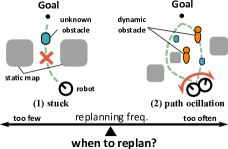
(a) Learning when to replan

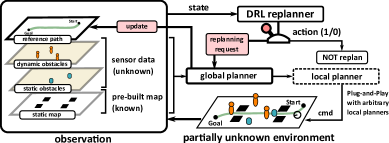
(b) Proposed system overview

Figure 1: Overview of our work. The hierarchical planning framework can partition difficulties between global and local planning. However, depending on the timing of the global planner’s replanning, negative behaviors can occur (Fig. 1). Specifically, in partially uncharted terrains that include unforeseen and dynamic obstacles on the pre-built static map, insufficient replanning frequency causes negative behaviors, i.e., (1) too low a replanning frequency can cause the robot to get stuck, while (2) excessive replanning can lead to path oscillation. Our objective is to control the timing of replanning adaptively to enable robust and efficient navigation of AMRs. To achieve this, we propose a replanning controller based on DRL (Fig. 1). The DRL replanner obtains an efficient and adaptive replanning strategy by training on the partially uncharted terrains and the hierarchical planning framework as its environment.

It’s a fact of life that things do not always go as planned. Whether the unexpected is a minor setback or a major obstacle, we must be ready to pivot and adjust our plans to ensure that we can still achieve our goals. The same applies to navigating autonomous mobile robots (AMRs). In real-world scenarios such as industrial factories or busy restaurants, the environment is filled with unforeseen obstacles or pedestrians that diverge from the pre-built map. To deal with such partially uncharted terrain, it becomes imperative to dynamically replan the pre-planned paths as needed.

In this paper, we delve into the timing of the replanning feature in the common hierarchical planning framework [1]. Carefully tuning the replanning feature is crucial in practice, as it can drastically change the behavior of AMRs and can affect navigation robustness and efficiency. When performed at the right time, replanning can enable goal-oriented and reactive motion in the presence of unforeseen and dynamic obstacles. However, improper replanning, for example, if done with too high or low a frequency, can also cause the AMRs to perform inefficient travel (e.g., path oscillation) or even get completely stuck, as shown in Fig. 1. Despite some relevant work [2, 3, 4, 5], an effective replanning strategy – more specifically when to execute replanning for robust and efficient navigation in partially uncharted terrain – remains an open question.

The primary contribution of this work is three-fold. First, we conduct a comprehensive experiment with simulated environments and systematically evaluate various replanning strategies commonly used in ROS 2 Navigation Stack [6]. We demonstrate that effective strategies are highly dependent on the map layouts as well as on the global and local planning algorithms, which implies the fact that the replanning strategy should be carefully designed and tuned for every single environment and choice of planning algorithm (Section V).

Second, we formulate a task of controlling the replanning timings for a global planner as a sequential decision-making problem using a Partially Observable Markov Decision Process (POMDP) [7] (Section III). We consider a replanning controller as a decision maker that determines whether to replan the reference path at every timestep. The conventional rule-based replanning strategies can be viewed as policies in the POMDP, which allows us to compare diverse replanning strategies in the unified framework.

Finally, based on the aforementioned POMDP, we derive a Deep Reinforcement Learning (DRL)-based replanning controller (hereafter referred to as DRL replanner) that learns to decide when to execute replanning for improving navigation robustness and efficiency in the current situation, as shown in Fig. 1 (Section IV). The DRL replanner is trained with a standard DRL algorithm such as a deep Q network [8]. Notably, the DRL replanner can act as a drop-in replacement for the rule-based replanning strategy in existing hierarchical planning frameworks. Our extensive experimental results have demonstrated that the proposed DRL replanner can achieve navigation that is as robust and efficient as, or better than, the currently best-performing strategies across various combinations of global and local planners in floor environments (Section V). These results have strong implications that well-controlled timing of replanning has the potential to achieve more robust and efficient navigation on the existing hierarchical planning frameworks by learning the environment-specific adaptive replanning strategy.

II RELATED WORK

While partitioning complex navigation problems into global and local planning can increase substitutability and reduce computational complexity through parallel processing, it can cause inefficient path replanning such as getting stuck and path oscillation, as illustrated in Fig. 1. Existing approaches to this issue can be broadly categorized into the following three types:

II-1 Replanning Timing Strategy

Existing planning systems typically employ rule-based replanning strategies that need to be hand-engineered to account for the characteristics of the environments and planners. Indeed, Murphy et al. found in their early study that the timing of replanning could be a salient factor for navigation performance [2]. Since then, various systems that replan at regular time intervals have emerged [1], and others adopt event-based rules, such as deviation from the reference path and detecting stuck [9, 10]. A practical software framework, ROS 2 Navigation Stack [6], provides behavior tree-based tools to allow engineers to implement various replanning strategies in a user-friendly manner. However, these manual design approaches require significant expertise to fine-tune, and it can be challenging to adjust replanning rules adaptively on the basis of the situation. This paper focuses for the first time on the evaluation and improvement of navigation performance through replanning strategies, which have not been adequately explored.

II-2 Reference Path Modification

Another approach to reducing inefficient path replanning is to modify the reference path in accordance with the current situation. For example, Tordesillas et al. proposed modifying a part of the reference path when the global planner significantly changes it from the current one [3]. While path modification is a valid approach, it highly depends on the nature of the global and local planners because the method and timing of the modification need to consider the shape of the reference path and the tracking performance of the local planner. Other works have also proposed updating the map dynamically [4, 5], but this is only effective when all obstacles remain static.

II-3 Navigation based on DRL

In recent years, DRL has become a popular approach for point-to-point navigation [11]. While many studies employ DRL to learn adaptive behavior for local planners in short-range navigation, some recent studies use DRL planners in conjunction with the reference paths generated by classical global planners in long-range navigation [12, 13, 14]. Most of these works, however, assume a standard periodic replanning of the global planner [9, 10, 15, 16]. An exception to this norm is the work by Wang et al., which does not necessitate replanning but is constrained to environments with a discrete action space [17]. Our work fundamentally differs from these approaches in that we propose a DRL-based adaptive replanning strategy for the global planner. Note that our approach is not limited to any particular type of local planner and can be used with a diverse array of planning methods. This adaptability is a key strength of our approach, allowing us to provide a flexible and versatile framework.

III HIERARCHICAL PLANNING FRAMEWORK

Our aim is to optimize the timing of replanning for robust and efficient navigation of AMRs in partially uncharted terrain due to unforeseen or dynamic obstacles that were not present when building an environment map. The replanning timing is desirable to be adaptively determined based on the nature of the hierarchical planning framework and observations of the robot’s surroundings obtained from sensors. we first provide an overview of a conventional hierarchical planning framework with a replanning feature and then formulate how to control the replanning timings as a sequential decision-making problem with a partially observable Markov decision process (POMDP) [7].

III-A Global and Local Planners

The typical configuration of a hierarchical planning framework consists of asynchronously operating global planner and local planner modules as shown in Fig. 1. The global planner (represented by $f_{\rm{gp}}$) computes a reference path to the given goal $\mathbf{p}^{g}\in\mathbb{R}^{2}$ from the robot position based on detected obstacles information estimated from a pre-built map and onboard sensor observation.

Specifically, $f_{\rm{gp}}$ receives obstacles information $\mathcal{M}_{t}$ and robot position $\mathbf{p}_{t}\in\mathbb{R}^{2}$ at time $t$ and produces a reference path as the sequence of 2D positions $\textbf{{P}}^{r}_{t+\Delta t_{d}}=\{\mathbf{p}^{r}_{0},\mathbf{p}^{r}_{1},\dots\}$ for time $t+\Delta t_{d}$: $\textbf{{P}}^{r}_{t+\Delta t_{d}}=f_{\rm{gp}}(\mathbf{p}^{g},\mathbf{p}_{t},\mathcal{M}_{t})$, where $\Delta t_{d}$ is the time delay due to the computation time for global planning. This calculation can generally become expensive as the size of pre-built maps increases, and $\Delta t_{d}$ can be larger than the control interval $\Delta t$. Note that $\Delta t_{d}$ can be estimated to some extent by using an any-time algorithm (e.g. any-time A* [18]) because such algorithms are interruptible. In practice, to consider the environmental change, global planning is performed repeatedly at a low frequency (~1 Hz) based on a predefined replanning strategy.

The local planner $f_{\rm{lp}}$ generates a more fine-grained and collision-free control command with a given control frequency (10 Hz~) to guide the robot along the reference path. The control command $\mathbf{v}^{\rm{cmd}}_{t}$ at time $t$ is calculated from the the latest reference path $\textbf{{P}}_{t^{*}}$, the robot position $\mathbf{p}_{t}$, and obstacle information $\mathcal{M}_{t}$ at time $t$, as $\mathbf{v}^{\rm{cmd}}_{t}=f_{\rm{lp}}(\textbf{{P}}_{t^{*}},\mathbf{p}_{t},\mathcal{M}_{t})$, where $t^{*}$ is delayed by at most $\Delta t_{d}$ from time $t$. The control command $\mathbf{v}^{\rm{cmd}}_{t}$ updates the physical motion of the robot for the control interval $\Delta t$.

III-B Formulation using POMDP

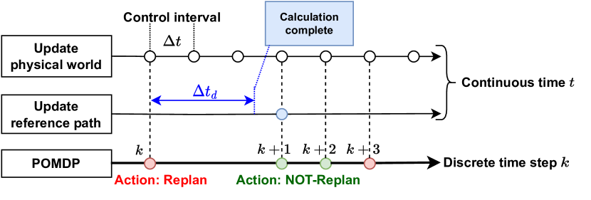
Figure 2: Time transition according to the replanning action.

The replanning of reference paths in the above hierarchical planning framework can be modeled by a deterministic POMDP as follows. Let $\Pi=(\mathcal{S},\mathcal{A},\mathcal{O},T,R,\Omega,\gamma)$ be the POMDP tuple consisting of state space $\mathcal{S}$, action space $\mathcal{A}$, observation space $\mathcal{O}$, transition function $T:\mathcal{S}\times\mathcal{A}\mapsto\mathcal{S}$, reward function $R:\mathcal{S}\times\mathcal{A}\mapsto\mathbb{R}$, observation model $\Omega:\mathcal{S}\mapsto\mathcal{O}$, and discount factor $\gamma\in[0,1)$.

The state $s_{k}$ includes the robot’s status (position, orientation, and past trajectory), the planners’ status (goal position and reference path), and the situation regarding surrounding obstacles at discrete time step $k$. While the states of the robot and planners are essentially observable, the surrounding situation is only partially observable from onboard sensors. As a result, the DRL replanner can only obtain observations $o_{k}\in\mathcal{O}$ based on the observation model $o_{k}=\Omega(s_{k})$ described in Section IV-B. The action $a_{k}\in\mathcal{A}$ is a binary decision of whether to replan or not at time step $k$. Specifically, $\mathcal{A}=\{a_{\rm{rep}},a_{\rm{not}}\}\in\mathbb{R}^{2}$, where $a_{\rm{rep}}$ requests the global planner $f_{\rm{gp}}$ to compute a new reference path and $a_{\rm{not}}$ does not, as illustrated in Fig. 1.

The state $s_{k}$ transitions to $s_{k+1}$ with the transition function $T(s_{k},a_{k})$. As the global and local planners run asynchronously and there is a delay due to the computation time for the global planning to output a new reference path, the transition function $T(s_{k},a_{k})$ needs to consider them. In the transition function, if the action is not replanning, the physical world is rolled out by the control command from the local planner with the current existing reference path at time step $k$ and returns the state after $\Delta t$, i.e., $T(s_{k},a_{\rm{not}})$ returns the state at the next time step $k+1=t+\Delta t$. If the action is replanning, the global planner immediately starts computing a new reference path at time step $k$. At the same time, the control command by the local planning rolls out the physical world based on the existing reference path until the computation is finished. Then, after computing the time delay $\Delta t_{d}$, the global planner outputs a new reference path, the local planner outputs a control command using the updated reference path, and the physical world returns a new state after $\Delta t$, i.e., $T(s_{k},a_{\rm{rep}})$ returns the state at $k+1=t+(\lfloor\frac{\Delta t_{d}}{\Delta t}\rfloor+1)\Delta t$, where $\lfloor\;\rfloor$ is a floor function. Overall, the interval of time steps in the POMDP is variable depending on the action, as shown in Fig. 2.

III-C Existing Replanning Strategies

In this work, we compare four types of rule-based replanning strategies available in ROS 2 Navigation Stack [6].

• Distance-based strategy determines replanning timings on the basis of traveled distance, e.g., every $d_{\rm{rep}}$ meters. That is, if $\Delta d_{k}\geq d_{\rm{rep}}$, then $a_{k}=a_{\rm{rep}}$, otherwise $a_{k}=a_{\rm{not}}$, where $\Delta d_{k}$ is the difference in travel from the last replanning and $d_{\rm{rep}}$ is a given parameter.

• Stuck-based strategy decides to execute replans when the robot stops at the same position for a given $\Delta t_{\rm{stuck}}$ seconds because the robot is considered to be stuck.

• Time-based strategy performs replanning at every fixed period of $\Delta t_{\rm{rep}}$ seconds. $\Delta t_{\rm{rep}}$ should be larger than $\Delta t_{d}$ to consider the computation time of global planning.

• Time-with-patience strategy adopts the time-based strategy when the robot is far from the goal ($>d_{\rm{patience}}$) and changes to stuck-based otherwise ($\leq d_{\rm{patience}}$), expecting to prevent a large detour near the goal.

Specific parameter settings will be presented in the experiment section. A key point here is that all of these existing strategies can be viewed as an instance of a hand-designed, deterministic policy for the aforementioned POMDP, which takes the current observation as input to decide if replanning should be done as an action.

IV ADAPTIVE REPLANNING USING DRL

Although a variety of replanning strategies are available, it remains unclear which one should be used and how the parameters should be tuned for a given environment as well as the choices of global and local planners. While replanning regularly with time-based and distance-based strategies at the highest possible frequency can allow the robot to constantly track the shortest distance path, doing so becomes superfluous if there are not many unforeseen obstacles in the pre-built map. Too much replanning could also cause path oscillation, especially when sampling-based global planners are utilized or the environment has many branching pathways. Moreover, since the computational cost of global planning increases as the environment becomes larger, it is important to execute replanning only when necessary. Adopting a stuck-based strategy is nonetheless nontrivial, because what can be defined as getting stuck will depend on the performance of local planners and the dynamics of surrounding obstacles, making it harder to manually tune the parameters of the strategy. To this end, we explore the possibility of leveraging deep reinforcement learning for adapting a replanning strategy to a given environment as well as the choices of planners.

IV-A DRL-based Replanning Controller

We derive a replanning controller that can learn from its previous navigation experiences to create a better replanning timing for navigation efficiency and robustness. As illustrated in Fig. 1, the replanner’s action is essentially the same as that of existing replanning strategies, i.e., binary actions indicating whether or not to execute replanning to produce a new reference path for the local planner after the current time step $k$. In other words, the replanner can potentially be utilized as a replacement module for the replanning strategy in existing planning frameworks, thus making it compatible with various combinations of planners and other modules.

IV-B Observation Design

We define the observation model $\Omega$ to include the status of surrounding obstacles, the reference path, the past trajectory, and the relative position of the target goal at time $k$. Note that these observations are also easily accessible in the practical navigation system. Specifically, the replanner receives an observation $o_{k}=[\textbf{{S}}_{k},\hat{\textbf{{P}}}^{r}_{k^{*}},\textbf{{T}}_{k},\mathbf{p}^{g}_{r}]=\Omega(s_{k})$ , where $\textbf{{S}}_{k}=\{\mathbf{s}_{i}\}_{i=0}^{n_{s}}\in\mathbb{R}^{2\times n_{s}}$ is the two-dimensional scan positions down-sampled to $n_{s}$ at time step $k$, $\hat{\textbf{{P}}}^{r}_{k^{*}}=\{\mathbf{p}_{i}\}_{i=0}^{n_{p}}\in\mathbb{R}^{2\times n_{p}}$ is the latest waypoints (reference path) down-sampled to $n_{p}$ at time step $k$, which is computed by the global planner, $\textbf{{T}}_{k}=\{\mathbf{t}_{i}\}_{i=0}^{n_{t}}\in\mathbb{R}^{2\times n_{t}}$ is the robot’s past trajectory downsampled to $n_{t}$ at time step $k$, which it does to make the replanner aware of stack and path oscillation situations. $\mathbf{p}^{g}_{r}=\mathbf{p}^{g}-\mathbf{p}_{k}\in\mathbb{R}^{2}$ is the relative position of a given goal, with goal position $\mathbf{p}^{g}$ and the robot position $\mathbf{p}_{k}$. That is, for our POMDP, $\mathcal{O}\in\mathbb{R}^{2\times(n_{o}+n_{p}+n_{t}+1)}$. Specific parameter settings will be described in the experiment section.

IV-C Reward Design

Designing an appropriate reward function is a crucial step to enable reinforcement learning. The reward function should reflect and quantify the replanner’s objective, that is, the efficiency (i.e., quick goals) and robustness (i.e., safety, collision-free) of the navigation in our case. As a unified metric that involves these criteria, we borrow the idea of success rate weighted by normalized goal time (SGT)  [19]. In the SGT, the score $s_{\rm{sgt}}^{i}$ of an episode $i$ is defined as follows:

$$s_{\rm{sgt}}^{i}=\frac{\mathbf{1}_{\rm{suc}}^{i}\rm{OT}_{i}}{\rm{{clip}(\rm{AT}_{i},\alpha\rm{OT}_{i}\beta\rm{OT}_{i})}}\text{, where }\rm{OT}_{i}=\frac{L_{\rm{path}}^{i}}{\rm{speed_{\rm{max}}}},$$ (1)

and $\mathbf{1}_{\rm{suc}}^{i}$ is a binary indicator function of success that the robot reaches the goal without collisions. $\rm{AT}_{i}$ and $\rm{OT}_{i}$ denote the actual and optimal traversal time as an indicator of the difficulty of the environment, respectively. The clip function clips AT within $\alpha$OT and $\beta$OT ($0<\alpha<\beta$) to reduce the influence of extremely easy or difficult episodes. $L_{\rm{path}}^{i}$ is the optimal (shortest) path length to the goal and is calculated using the observation at the initial time by the Dijkstra method. $\rm{speed}_{\rm{max}}$ is a maximal speed of the robot. We can define the reward function as $R(s_{t},a_{t})=\mathbf{1}_{\mathbf{p}_{t}=\mathbf{p}^{g}}s_{\rm{sgt}}^{i}$, where $\mathbf{1}_{\mathbf{p}_{t}=\mathbf{p}^{g}}$ is a binary function indicating that the robot reaches the goal. Note that episodes are terminated when the robot collides or reaches the goal. Although the SGT in (1) returns a non-zero score when an episode ends by reaching a given time limit, the reward at the time limit is zero to avoid conflicts with the handling of time limits in the bootstrapping of training [20].

IV-D Learning Algorithm

To train the replanning controller, a DRL algorithm that can handle binary actions would be sufficient. We opt to use the popular deep Q-network (DQN) [8] algorithm that approximates the Q-function with a deep neural network (i.e., Q-network) and obtains an optimal policy that maximizes the Q-values.

A key point here is that the actual timing at which replanning is necessary appears only sparsely during a long travel. In other words, most of the gathered experiences, i.e., transitions, may not necessarily be useful for learning appropriate replanning timings. To address this issue, we employ a prioritized experience replay (PER) buffer [21] that gives different weights for each experience in the loss function based on its priority. Specifically, we use the priority $p_{k}$ based on the difference of Q-values between whether or not replanning was performed,

$$p_{k}=\|Q_{\theta}(s_{k},a_{\rm{rep}})-Q_{\theta}(s_{k},a_{\rm{not}})\|.$$ (2)

Here, higher differences indicate that replanning at the corresponding timing makes the SGT better (or worse), and thus should be emphasized more in the replay buffer. This definition of priority is more intuitive and effective than the conventional priority based on TD-error (i.e., $p_{k}=\|Q_{\theta}(s_{k},a_{k})-(R_{i}(s_{k},a_{k})+\gamma\max_{a}Q^{\tau}_{\theta^{-}}(s_{k+1},a))\|$), as will be shown empirically in our experimental results.

V EXPERIMENTS

We conduct a comprehensive simulation study to systematically evaluate the existing planning strategies presented in Sec. III-C and the DRL replanner proposed in Sec. IV.

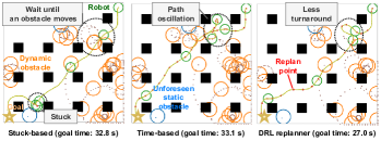
(a) A simulation result for 16-pillar map

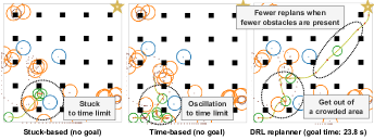
(b) A simulation result for 25-pillar map

Figure 3: Selected simulation results. In Fig. 3, the stuck-based and time-based replanning strategies had difficulties in dealing with dynamic obstacles, while the proposed DRL replanner avoided them efficiently, resulting in reaching the goal about six seconds faster than the time-based replanning. In Fig. 3, the stuck-based and time-based replanning strategies failed to reach the goal due to the movement of dynamic obstacles, while the proposed DRL replanner reached the goal by replanning at key points and adapting to the situation.

V-A Environment Setup

We developed three-floor navigation environments in continuous action space with different numbers of no-entry areas for the robot (nine, 16, and 25 uniformly lined regions sized 1.5, 1.0, and 0.5 meters, respectively; see Fig. 3). Ten dynamic or unforeseen static obstacles spawn with random initial positions and velocities in each environment. The robot needs to reach a goal while avoiding collisions with the obstacles and detouring around the no-entry areas. While the no-entry areas are encoded in the pre-built map and are considered when executing global planning, the obstacles are not. To enable the dynamic obstacles to be widely distributed throughout the field, we assume that the dynamic obstacles can move over the no-entry areas.

The behavior of the dynamic obstacles is modeled as a social force model (SFM) [22] or reactive stop model (RSM) that predicts its motion for several (e.g. 3) seconds as a point mass model and stops in the case of collision. SFM simulates an agent that recognizes and avoids the robot, while RSM simulates an agent that does not avoid the robot. These models are randomly selected for each obstacle and represent dynamic obstacles that may or may not yield to the robot. In these cases, where all dynamic obstacles give the robot the way based on the SFM, the robot does not need to replan and detour to reach the goal. However, such cases are rare in the real world.

V-B Setup of Robot and Planners

We simulate a wheeled robot modeled as a circle with a fixed radius (1.0 m). The simulated robot follows the non-holonomic kinematics of the differential wheeled model characterized by a maximum velocity (1.0 m/s) and angular velocity (1.0 rad/s) at each control interval $\Delta t=0.1$ s. The initial and goal positions are sampled randomly from one of the corners of the environment.

As the hierarchical planning system described in Sec. III, we implemented Dijkstra, rapidly-exploring random tree* (RRT*) [23], and probabilistic roadmaps (PRM) [24] as the global planners, and implemented the dynamic window approach (DWA) [25] and sampling-based model predictive control (MPC) [26] as the local planners that compute the target velocity of the robot. Although these modules generally run asynchronously, we process them synchronously here for reproducibility. That is, the time delay of the global planning described in section III is reproduced as a given constant time: $\Delta t_{d}=1$ s.

V-C Replanning Strategy Setup

We implemented the rule-based replanning strategy with manually tuned parameters as described in Sec. III-C, with $d_{\rm{rep}}=1$ m, $\Delta t_{\rm{stuck}}=3$ s, $\Delta t_{\rm{rep}}=1$ s, and $d_{\rm{patience}}=3$ m. Also, the dimension of the observation space described in Sec. IV-B is $62$, with $n_{s}=20$, $n_{p}=5$, and $n_{t}=5$. The replanner was trained on each map layout using the DQN algorithm described in Sec. IV-D based on stable-baselines3 [27]. We trained the Q network using an Adam optimizer. The network architecture is a multi-layer perceptron with [128, 128] intermediate layers, the learning rate is 0.0001, the batch size is 128, the buffer size is 100k, and the discount factor $\gamma$ is 0.99 for 100k timesteps (over 1k episodes).

V-D Evaluation Metrics

To evaluate the effectiveness of our RL-based replanning compared to the rule-based strategies, we simulated 100 trials of the navigation. The following five metrics are used for a quantitative evaluation of the navigation performance:

• SR: The success rate over 100 trials, where success is defined as the robot reaching the goal without collision.

• CR: The collision rate over 100 trials.

• SGT: The average success rate weighted normalized goal time in (1) ($\alpha=4,\beta=8$).

• SPL: The average success rate weighted normalized path length defined as $\rm{SPL}=\frac{1}{N}\sum^{N}_{i=0}\frac{\mathbf{1}_{\rm{suc}}^{i}\rm{AL}_{i}}{\max(\rm{AL}_{i},\rm{OL}_{i})}$ , where $N$ is the number of trials ($N=100$), $\mathbf{1}_{\rm{suc}}^{i}$ is a binary indicator function of success, and AL and OL denote the actual and optimal traversal length as an indicator of the difficulty of the environment, respectively. The SPL evaluates the navigation’s efficiency with respect to the traveled distance.

• NR: The number of replanning over 100 trials.

TABLE I: Simulation Results

No. of no-entry areas	9					16					25
Metrics	SR$\uparrow$	CR$\downarrow$	SGT$\uparrow$	SPL$\uparrow$	NR$\downarrow$	SR$\uparrow$	CR$\downarrow$	SGT$\uparrow$	SPL$\uparrow$	NR$\downarrow$	SR$\uparrow$	CR$\downarrow$	SGT$\uparrow$	SPL$\uparrow$	NR$\downarrow$
No replan	33	11	0.461	0.330	–	27	10	0.439	0.270	–	24	4	0.418	0.240	–
Distance-based	66	13	0.529	0.572	2202	62	12	0.509	0.547	2186	82	12	0.561	0.705	1995
Stuck-based	67	12	0.511	0.619	914	64	13	0.493	0.605	739	71	6	0.482	0.658	818
Time-based	64	15	0.527	0.570	3063	70	10	0.538	0.615	3076	79	12	0.562	0.688	2671
Time w/ patience	64	15	0.529	0.570	2953	70	10	0.540	0.615	2956	79	12	0.564	0.688	2558
DRL replanner (ours)	64	10	0.532	0.567	1361	77	4	0.563	0.668	2577	87	6	0.600	0.751	2066

• SR, CR, SGT, SPL, and NR mean success rate [%], collision rate [%], success rate weighted goal time, success rate weighted path length, and the number of replanning operations, respectively. SGT and SPL show the time and path efficiency of the navigation. Dijkstra and DWA planners are used for global and local planners in the training and evaluation.

V-E Experimental Results

V-E1 Quantitative Comparisons

Table I lists the quantitative evaluation results of 100 trials for each map layout with Dijkstra and DWA planners. Overall, we confirmed that the baseline strategies, i.e., distance-based, stuck-based, time-based, and time w/ patience, show quite different tendencies for each environment. The stuck-based strategy demonstrates a consistently lower number of replanning operations (NR) and consequently outperforms the other methods in terms of SPL (i.e., shorter travel distance on average) in the easiest environment with a lower number of no-entry areas ($N=9$). For more complicated environments with $N=16,25$, the distance-based and time-based strategies become more robust and efficient. This is arguable because these methods periodically perform replanning to refine the reference path. Nevertheless, these results come at the cost of an increase in the number of replanning operations–in other words, more computational resources are required. In contrast, the DRL replanner, which learns from its experiences to seek better-replanning timings, works comparably well or sometimes substantially better than the other rule-based strategies in each environment. For the $N=9$ environment, the DRL replanner was slightly outperformed by the stuck-based strategy but still able to perform on par with the remaining baselines with much fewer replanning operations.

V-E2 Qualitative Results

Figure 3 visualizes some selected navigation results with the stuck-based and time-based strategies as well as the DRL replanner. Each method demonstrates its own unique behavior. For example, with the stuck-based strategy in Fig. 3, the robot simply waited until a dynamic obstacle was out of its way near the starting point and then performed the replanning around the goal by getting stuck at the static obstacle. In contrast, the time-based strategy periodically updated the reference path, but this sometimes resulted in path oscillation as shown in Fig. 3. This happens when the frequency of replanning is unnecessarily high compared to the actual need. Figure 3 presents a more challenging case where both stuck-based and time-based replanning failed to work. In contrast, the DRL replanner was able to learn to adapt its replanning strategy to the given environments and performed replanning only when necessary. Indeed, fewer replanning operations were executed in less crowded areas, which resulted in overall shorter travels compared to the stuck-based and time-based strategies.

V-E3 Results with Different Planners

TABLE II: Comparison of performance by planners

GP	LP	Method	SR	CR	SGT	SPL	NR
Dijkstra	DWA	Stuck-based	64	13	0.493	0.605	739
		Time-based	70	10	0.538	0.615	3076
		DRL	77	4	0.563	0.668	2577
Dijkstra	MPC	Stuck-based	70	10	0.434	0.483	298
		Time-based	75	8	0.487	0.560	2181
		DRL	82	8	0.502	0.601	1582
PRM	DWA	Stuck-based	66	10	0.537	0.617	808
		Time-based	72	13	0.542	0.623	2958
		DRL	74	7	0.570	0.647	2293
RRT*	DWA	Stuck-based	65	10	0.473	0.537	661
		Time-based	57	6	0.446	0.441	3758
		DRL	58	5	0.445	0.443	2801

• GP and LP are global and local planners, respectively.

Table II lists the results of Dijkstra–MPC, PRM–DWA, and RRT*–DWA combinations of global and local planners in addition to Dijkstra–DWA reported in the previous section. Again, we confirmed that the proposed DRL replanner could learn to adapt itself to the choices of planners, except when RRT* was used. One possible reason for the degraded performance with RRT* is its stochastic nature that gives not exactly consistent paths upon replanning, regardless of the current observation. This would make learning the replanning strategy harder than when combined with the other global planners. Note that PRM can produce a consistent path once the roadmap is created by random sampling, making it a better choice when a sampling-based global planner is necessary for larger environments.

V-E4 Ablation Study

TABLE III: Comparison of results with RL algorithms

RL algorithm	SR	CR	SGT	SPL	NR
w/o PER	69	12	0.514	0.595	2396
w/ PER-TDerror	69	9	0.541	0.608	2414
w/ PER-Qerror (ours)	77	4	0.563	0.668	2577

• Dijkstra and DWA planners are used as GP and LP on the 16-pillar map.

Finally, Table III compares other reinforcement learning techniques that were not used in the proposed method. Specifically, we investigated how the overall performances change if the prioritized experience replay was not used (w/o PER) or if the priority was determined using TD error (w/ PER-TDerror). Although the number of replanning operations (NR) was almost the same, there was a substantial difference in the success rate (SR) and consequently in other metrics such as SGT and SPL. These findings suggest that changes in Q-value can function as a salient clue for replanning, and using them as the priority of experiences leads to more efficient training of the replanning controller.

VI CONCLUSION AND LIMITATIONS

This paper is the first to delve into when to replan the reference path in a common hierarchical planning framework. We propose the DRL-based solution that addresses inefficiencies caused by the conventional rule-based replanning strategy. Our simulation results demonstrate that our proposed DRL-based replanning strategy achieves similar or better efficiency than the other rule-based strategies in the maps with branching pathways and dynamic obstacles. We believe that these results have strong implications for designing replanning strategies in autonomous robot navigation. In this study, we used simple floor plans to highlight the effect of static and dynamic obstacles. Our proposed framework can easily be extended to other scenarios, such as maze-like spaces or real-world maps, which we plan to explore in future work.

References

- [1] O. Brock and O. Khatib, “High-speed navigation using the global dynamic window approach,” in International Conference on Robotics and Automation, vol. 1. IEEE, 1999, pp. 341–346.
- [2] R. R. Murphy, A. Marzilli, and K. Hughes, “When to explicitly replan paths for mobile robots,” in International Conference on Robotics and Automation, vol. 4. IEEE, 1997, pp. 3519–3525.
- [3] J. Tordesillas, B. T. Lopez, J. Carter, J. Ware, and J. P. How, “Real-time planning with multi-fidelity models for agile flights in unknown environments,” in International Conference on Robotics and Automation. IEEE, 2019, pp. 725–731.
- [4] H. Zha, K. Tanaka, and T. Hasegawa, “Detecting changes in a dynamic environment for updating its maps by using a mobile robot,” in International Conference on Intelligent Robot and Systems, vol. 3. IEEE/RSJ, 1997, pp. 1729–1734.
- [5] H. Oleynikova, Z. Taylor, R. Siegwart, and J. Nieto, “Safe local exploration for replanning in cluttered unknown environments for microaerial vehicles,” IEEE Robotics and Automation Letters, vol. 3, no. 3, pp. 1474–1481, 2018.
- [6] S. Macenski, T. Moore, D. V. Lu, A. Merzlyakov, and M. Ferguson, “From the desks of ros maintainers: A survey of modern & capable mobile robotics algorithms in the robot operating system 2,” Robotics and Autonomous Systems, p. 104493, 2023.
- [7] L. P. Kaelbling, M. L. Littman, and A. R. Cassandra, “Planning and acting in partially observable stochastic domains,” Artificial intelligence, vol. 101, no. 1-2, pp. 99–134, 1998.
- [8] V. Mnih, K. Kavukcuoglu, D. Silver, A. A. Rusu, J. Veness, M. G. Bellemare, A. Graves, M. Riedmiller, A. K. Fidjeland, G. Ostrovski, et al., “Human-level control through deep reinforcement learning,” nature, vol. 518, no. 7540, pp. 529–533, 2015.
- [9] K. Ota, Y. Sasaki, D. K. Jha, Y. Yoshiyasu, and A. Kanezaki, “Efficient exploration in constrained environments with goal-oriented reference path,” in International Conference on Intelligent Robots and Systems. IEEE/RSJ, 2020, pp. 6061–6068.
- [10] L. Kästner, X. Zhao, T. Buiyan, J. Li, Z. Shen, J. Lambrecht, and C. Marx, “Connecting deep-reinforcement-learning-based obstacle avoidance with conventional global planners using waypoint generators,” in International Conference on Intelligent Robots and Systems. IEEE/RSJ, 2021, pp. 1213–1220.
- [11] L. Dong, Z. He, C. Song, and C. Sun, “A review of mobile robot motion planning methods: from classical motion planning workflows to reinforcement learning-based architectures,” arXiv preprint arXiv:2108.13619, 2021.
- [12] A. Faust, K. Oslund, O. Ramirez, A. Francis, L. Tapia, M. Fiser, and J. Davidson, “PRM-RL: Long-range robotic navigation tasks by combining reinforcement learning and sampling-based planning,” in International Conference on Robotics and Automation. IEEE, 2018, pp. 5113–5120.
- [13] H.-T. L. Chiang, J. Hsu, M. Fiser, L. Tapia, and A. Faust, “RL-RRT: Kinodynamic motion planning via learning reachability estimators from RL policies,” IEEE Robotics and Automation Letters, vol. 4, no. 4, pp. 4298–4305, 2019.
- [14] A. Pokle, R. Martín-Martín, P. Goebel, V. Chow, H. M. Ewald, J. Yang, Z. Wang, A. Sadeghian, D. Sadigh, S. Savarese, et al., “Deep local trajectory replanning and control for robot navigation,” in International Conference on Robotics and Automation. IEEE, 2019, pp. 5815–5822.
- [15] L. Kästner, T. Buiyan, L. Jiao, T. A. Le, X. Zhao, Z. Shen, and J. Lambrecht, “Arena-Rosnav: Towards deployment of deep-reinforcement-learning-based obstacle avoidance into conventional autonomous navigation systems,” in International Conference on Intelligent Robots and Systems. IEEE/RSJ, 2021, pp. 6456–6463.
- [16] B. Angulo, A. Panov, and K. Yakovlev, “Policy optimization to learn adaptive motion primitives in path planning with dynamic obstacles,” IEEE Robotics and Automation Letters, vol. 8, no. 2, pp. 824–831, 2022.
- [17] B. Wang, Z. Liu, Q. Li, and A. Prorok, “Mobile robot path planning in dynamic environments through globally guided reinforcement learning,” IEEE Robotics and Automation Letters, vol. 5, no. 4, pp. 6932–6939, 2020.
- [18] M. Likhachev, G. J. Gordon, and S. Thrun, “ARA*: Anytime A* with provable bounds on sub-optimality,” Advances in neural information processing systems, vol. 16, 2003.
- [19] X. Xiao, Z. Xu, Z. Wang, Y. Song, G. Warnell, P. Stone, T. Zhang, S. Ravi, G. Wang, H. Karnan, et al., “Autonomous ground navigation in highly constrained spaces: Lessons learned from the benchmark autonomous robot navigation challenge at ICRA 2022,” Robotics & Automation Magazine, vol. 29, no. 4, pp. 148–156, 2022.
- [20] F. Pardo, A. Tavakoli, V. Levdik, and P. Kormushev, “Time limits in reinforcement learning,” in International Conference on Machine Learning. PMLR, 2018, pp. 4045–4054.
- [21] T. Schaul, J. Quan, I. Antonoglou, and D. Silver, “Prioritized experience replay,” in International Conference on Learning Representations, 2016.
- [22] D. Helbing and P. Molnar, “Social force model for pedestrian dynamics,” Physical review E, vol. 51, no. 5, p. 4282, 1995.
- [23] S. Karaman and E. Frazzoli, “Sampling-based algorithms for optimal motion planning,” The international journal of robotics research, vol. 30, no. 7, pp. 846–894, 2011.
- [24] L. E. Kavraki, P. Svestka, J.-C. Latombe, and M. H. Overmars, “Probabilistic roadmaps for path planning in high-dimensional configuration spaces,” Transactions on Robotics and Automation, vol. 12, no. 4, pp. 566–580, 1996.
- [25] D. Fox, W. Burgard, and S. Thrun, “The dynamic window approach to collision avoidance,” IEEE Robotics & Automation Magazine, vol. 4, no. 1, pp. 23–33, 1997.
- [26] A. Muraleedharan, H. Okuda, and T. Suzuki, “Real-time implementation of randomized model predictive control for autonomous driving,” IEEE Transactions on Intelligent Vehicles, vol. 7, no. 1, pp. 11–20, 2021.
- [27] A. Raffin, A. Hill, A. Gleave, A. Kanervisto, M. Ernestus, and N. Dormann, “Stable-baselines3: Reliable reinforcement learning implementations,” Journal of Machine Learning Research, vol. 22, no. 268, pp. 1–8, 2021.