Thermodynamic properties of small flares in the quiet Sun observed by H$\alpha$ and EUV: plasma motion of the chromosphere and time evolution of temperature / emission measure

Abstract

Small flares frequently occur in the quiet Sun. Previous studies have noted that they share many common characteristics with typical solar flares in active regions. However, their similarities and differences are not fully understood, especially their thermal properties. In this study, we performed imaging spectroscopic observations in the H$\alpha$ line taken with the Solar Dynamics Doppler Imager on the Solar Magnetic Activity Research Telescope (SMART/SDDI) at the Hida Observatory and imaging observations with the Atmospheric Imaging Assembly onboard Solar Dynamics Observatory (SDO/AIA). We analysed 25 cases of small flares in the quiet Sun over the thermal energy range of $10^{24}-10^{27}\,\mathrm{erg}$, paying particular attention to their thermal properties. Our main results are as follows: (1) We observe a redshift together with line centre brightening in the H$\alpha$ line associated with more than half of the small flares. (2) We employ differential emission measure analysis using AIA multi-temperature (channel) observations to obtain the emission measure and temperature of the small flares. The results are consistent with the Shibata & Yokoyama (1999, 2002) scaling law. From the scaling law, we estimated the coronal magnetic field strength of small flares to be 5 –15 G. (3) The temporal evolution of the temperature and the density shows that the temperature peaks precede the density peaks in more than half of the events. These results suggest that chromospheric evaporations/condensations play an essential role in the thermal properties of some of the small flares in the quiet Sun, as does for large flares.

1 Introduction

Small flares are frequently observed throughout the solar atmosphere. Depending on their energy, they have been named microflares ($10^{26}-10^{29}\,\mathrm{erg}$) or nanoflares ($10^{23}-10^{26}\,\mathrm{erg}$). In this paper, we focus on small flares in the quiet Sun (QS) corona with energies of $10^{24}-10^{27}\,\mathrm{erg}$ (hereafter “small flares”).

Various instruments have observed brightenings associated with small flares for more than 20 years (Krucker et al., 1997; Krucker & Benz, 1998; Berghmans et al., 1998; Aschwanden et al., 2000; Parnell & Jupp, 2000; Benz & Krucker, 2002; Joulin et al., 2016; Chitta et al., 2021a; Purkhart & Veronig, 2022). Numerous studies have investigated whether small flares have the required energies to heat the solar corona (Parker, 1988). It is believed that the nanoflares observed with the current telescope resolution do not have enough energy to heat the steady corona (Chitta et al., 2021a). In contrast, we have not yet reached a consensus on whether nanoflares that are too small to be captured by the current resolution can be responsible for coronal heating. For nanoflares to have a significant contribution to coronal heating, the power-law index between the flare frequency $dN/dE$ and the flare energy $E$ must be smaller than $-2$ ($dN/dE\propto E^{\alpha}$, $\alpha<-2$) (Hudson, 1991). In recent observations using the Atmospheric Imaging Assembly onboard the Solar Dynamics Observatory (SDO/AIA) (Pesnell et al., 2012; Lemen et al., 2012), Purkhart & Veronig (2022) reported a power-law index smaller than $-2$ ($\alpha=-2.28\pm 0.03$), whilst Joulin et al. (2016) reported a power-law index larger than $-2$ ($\alpha=-1.73$ in the QS). Further understanding of the mechanism of small flares in the QS is crucially important for resolving this open question.

Small flares in the QS at coronal temperatures often accompany small eruptions at chromospheric temperatures (called “minifilament"). Minifilament eruptions were first reported in the 1970s (Moore et al., 1977; Labonte, 1979). Multi-wavelength observations using chromospheric and Extreme Ultraviolet (EUV) lines in the 2000s showed that they typically accompany coronal small flares (Sakajiri et al., 2004; Ren et al., 2008). These studies also reported that minifilament eruptions were associated with magnetic flux cancellation in the photosphere. Minifilament eruptions are often reported to be associated with jets (e.g., Sterling et al., 2015). Madjarska et al. (2020) reported simultaneous brightening in the H$\alpha$ line and EUV accompanied by a minfilament eruption. Galsgaard et al. (2019) reproduced the coronal magnetic field at the location of a microflare and minifilament eruption in a coronal bright point (CBP, Madjarska, 2019) using the non-linear force-free field (NLFFF) method. They found that twisted magnetic field lines (flux ropes) form at the minifilament eruption location. This is similar to the magnetic morphology of solar flares (e.g., Jiang et al., 2013; Inoue et al., 2014; Yamasaki et al., 2022). Kontogiannis et al. (2020) and Panesar et al. (2022) performed spectroscopic observations of chromospheric lines (H$\alpha$ and Mg II, respectively) and reported that brightenings and downflow in the chromosphere are observed in response to EUV brightenings. Jin et al. (2021) observed microflares with minifilament eruptions using the AIA. They found that the AIA 304 Å  light curve’s peak precedes the coronal emission’s peak by 2 or 3 minutes. This trend suggests a Neupert effect in large flares (Neupert, 1968); that is, the hard X-ray light curve corresponds to the time derivative of the soft X-ray light curve. All these properties support the interpretation that small flares in the QS with minifilament eruptions are miniature versions of typical solar flares associated with filament eruptions.

Recent observations by the Extreme Ultraviolet Imager (EUI, Rochus et al., 2020) onboard Solar Orbiter (SO, Müller et al., 2020) revealed small brightenings in the QS that were named “campfires” (Berghmans et al., 2021). The average temperature of these brightenings was estimated at $\log T=6.1$, which is consistent with other brightenings observed in the QS in the past. Berghmans et al. (2021) and Zhukov et al. (2021) compared their length and height using triangulation with SO/EUI and SDO/AIA. These studies found that the height was larger than the length, which suggests that the brightenings occur only near the apex of the loops. Panesar et al. (2021) found that campfires are often associated with magnetic flux cancellation and dark eruptions seen in EUV emission that may correspond to minifilament. With recent improvements in numerical simulation techniques, realistic simulations have been performed to reproduce the EUI brightenings (e.g., Tiwari et al., 2022; Panesar et al., 2023). Chen et al. (2021) performed the 3D radiation magnetohydrodynamics simulation with a QS parameter and reproduced brightenings with similar properties to the observed features. They found that these brightenings are caused by heating the cool and dense plasma to 1 MK. This heating is due to magnetic reconnection that occurs below the transition region. This mechanism differs from the brightening mechanism involving chromospheric evaporation when reconnection occurs in the corona.

Although small flares in the QS have been studied intensively, the similarities and differences with the physical mechanisms of typical solar flares are not fully understood. In particular, we do not fully understand how small-scale reconnection events affect the chromosphere. Several minifilament eruption studies have reported brightening in the chromosphere with EUV brightening (e.g., Sakajiri et al., 2004; Madjarska et al., 2020). However, only Kontogiannis et al. (2020), Madjarska et al. (2022), and Panesar et al. (2022) performed spectroscopic observations, and all studies analysed only one event. Investigating whether small flares in the QS also show red asymmetry in chromospheric lines observed during large flares (Ichimoto & Kurokawa, 1984; Canfield et al., 1990) may help us understand the heating mechanism at work (Ashfield & Longcope, 2021). To the best of our knowledge, there exist no studies clearly showing chromospheric evaporation at work during small flares in the QS. A comparison with scaling law studies of flares in active regions is also expected to help investigate the physical mechanism of small flares in the QS (e.g., Shibata & Yokoyama, 1999, 2002; Namekata et al., 2017b; Aschwanden, 2020). If the observations are consistent with the scaling law, we can expect the same physical mechanisms at work in small flares in the QS as in large flares.

In this study, we performed H$\alpha$ line imaging and spectroscopic analysis together with coronal EUV imaging analysis of more than 20 small flares in the QS. We aimed to improve our understanding of the thermal evolution of small flares in the QS and their impact on the chromosphere. This paper uses the term "small flare" while referring to brightening phenomena in EUV emission at coronal temperature.

2 Observations and data processing

We observed the chromosphere using the Solar Dynamics Doppler Imager (SDDI: Ichimoto et al., 2017) on the Solar Magnetic Activity Research Telescope (SMART: UeNo et al., 2004) at the Hida Observatory of Kyoto University. SDDI performs H$\alpha$ imaging spectroscopy observations of the full solar disk with a time resolution of 12 s and a pixel size of 1.23 arcsec. In this study, we took H$\alpha$ images at 25 wavelengths from H$\alpha-3.0$ Å  to H$\alpha+3.0$ Å  with a constant wavelength step of 0.25 Å. The data were processed with dark and flat field corrections. We used a position angle for the Sun to rotate the SDDI data and make the upward direction of the image orientate towards the solar north pole. We confirmed that the rotated SDDI data and AIA level 1.5 data generated by $\mathsf{sunpy}$’s $\mathsf{aiapy.calibrate}$ (Barnes et al., 2020) were aligned with an accuracy of less than $1.0\,\mathrm{arcsec}$.

We analysed small flares with plasma eruptions at chromospheric temperatures captured by SDDI and AIA from 21:56:17 UT on September 6, 2019, to 8:32:40 UT on September 7, 2019. All of these events occurred in the QS. We excluded near-limb events and analysed 25 small flares. These events are the same as our previous study investigating the relationship between chromospheric ejections and small flare energies in the QS (Kotani et al., 2023). As Kotani et al. (2023) described, these 25 events were selected for having observed ejecta near the disc centre in the wing difference images obtained by SMART/SDDI. Previous studies have reported that small flares in the QS are often accompanied by dark ejecta (Panesar et al., 2021). Our present analysis is specifically focused on events exhibiting dark ejecta, which may limit the generalizability of our findings to other events. Further investigations are required to establish the broader applicability of our results beyond the specific subset of events analysed in this study.

We used SDO/AIA data to study the properties of small flares. We checked images of the 304 Å  and 6 coronal channels (94 Å, 131 Å, 171 Å, 193 Å, 211 Å, and 335 Å). The method used to determine the physical quantities (flare spatial scale, temperature, emission measure, and electron number density) of small flares was the same as in our previous study (Kotani et al., 2023) using differential emission measure (DEM) analysis (Hannah & Kontar, 2012). We defined the flare duration as the time between the brightening beginning and returning to its original intensity in the AIA 193 Å  images. Thus, even if multiple brightening peaks are included, they are assumed to be the duration of a single event.

We used the Helioseismic and Magnetic Imager (HMI: Scherrer et al., 2012) onboard SDO to study the photospheric magnetic field of the small flares. We used magnetograms with a 45 seconds cadence because of the short duration of the events.

3 results

3.1 Overview

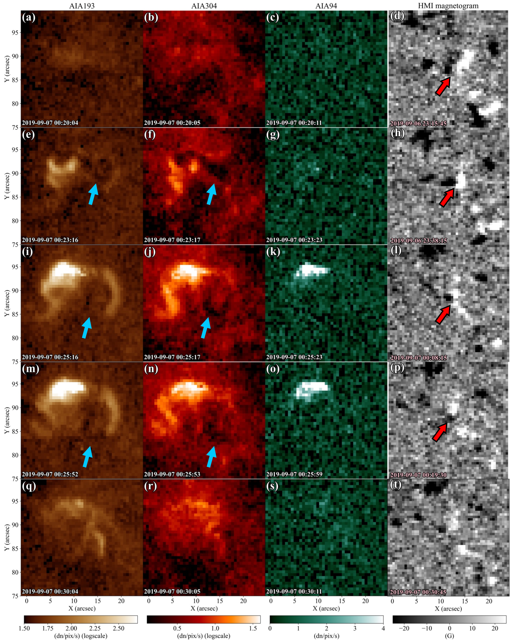
Figure 1: The time evolution of a typical event (event 4 in Table 1) in AIA and HMI images. The three left columns show the time evolution in AIA 193 Å, 304 Å, and 94 Å, respectively. Light blue arrows indicate dark ejecta. The right column shows the time variation of HMI magnetograms. Red arrows indicate dipole magnetic fields that indicate cancellation. HMI images are corrected for the effect of the solar rotation to track the field of view of the panel (t). Note that the AIA and HMI images on the same row are at different times.

In Fig. 1, we show a typical example of an event analysed in this study. We can see a brightening appearing in the AIA images from Fig. 1. The dark ejecta can be seen in the AIA 193 Å  and 304 Å  images (Figs. 1e, f, i, j, m, and n). The brightening in AIA 94 Å  is weaker than in 193 Å (Figs. 1k and o). We can see from the HMI images that magnetic field polarities converge and cancel (Figs. 1d, h, l, and p). We also confirmed from the broader field of view images that this event occurred at the network boundary. All these properties are consistent with previous studies (e.g., Sakajiri et al., 2004; Panesar et al., 2021).

Table 1: Parameters of small flares analysed in this study.

event	peak time (UT)	X (arcsec)	Y (arcsec)	$L\,\mathrm{(km)}^{\mathrm{a}}$	$t_{\mathrm{dur}}\,\mathrm{(s)}^{\mathrm{b}}$	$\log(T_{\mathrm{DEM}}/[\mathrm{K}])^{\mathrm{c}}$	$n$ $(10^{9}\,\mathrm{cm}^{-3})^{\mathrm{d}}$	$v_{\mathrm{red}}$ $(\mathrm{km}\,\mathrm{s}^{-1})^{\mathrm{e}}$	FCf	comments
1	9/6 22:02:16	-350	230	1100	360	6.12	2.12		Y	MBg
2	9/6 23:35:16	-260	-360	1500	360	6.14	2.54	2.82	Y	jet?
3	9/7 00:09:16	-70	-450	2400	636	6.19	3.19	4.83	Y	CBP, jet
4	9/7 00:25:52	10	90	3800	516	6.17	1.71	2.03	Y
5	9/7 01:32:16	320	470	1000	408	6.09	2.31	0.97	Y	jet, MB
6	9/7 02:11:52	40	-450	2800	1008	6.17	2.94	4.48	Y	CBP
7	9/7 02:18:16	620	-180	2200	540	6.12	1.74		Y
8	9/7 02:25:16	-420	480	3600	912	6.14	1.93		Y	MB
9	9/7 02:32:28	-540	-40	1200	84	6.12	1.67	2.47	Y
10	9/7 03:17:04	610	510	2700	180	6.20	1.78		Y	CBP, jet, MB
11	9/7 03:20:28	-100	-50	3200	900	6.13	1.79		Y	jet, MB
12	9/7 03:47:28	-70	260	4300	1044	6.17	1.55		Y	CBP, jet, MB
13	9/7 05:28:52	200	-290	2700	312	6.21	1.79	4.40	A	CBP
14	9/7 05:38:52	-220	290	2200	360	6.15	1.91	1.50	Y	CBP?, jet, MB
15	9/7 05:47:28	710	160	6200	1188	6.15	2.96	4.22	Y	CBP, jet, MB
16	9/7 06:03:16	340	-480	1300	252	6.13	2.53	5.08	Y	CBP, jet?
17	9/7 06:48:28	-320	-540	1600	360	6.11	2.11		Y
18	9/7 06:50:40	-420	430	1100	600	6.11	1.93		Y	MB
19	9/7 06:49:28	-30	-510	2800	264	6.07	1.39	4.56	Y	jet, MB
20	9/7 06:56:52	140	-790	2400	156	6.13	1.53		Y	CBP
21	9/7 07:06:52	650	-100	3500	548	6.13	1.46		Y	jet
22	9/7 07:13:52	-270	-660	1200	408	6.11	2.80	3.50	A	MB
23	9/7 07:27:40	490	-30	1300	216	6.16	2.44	3.95	Y	MB
24	9/7 07:35:16	190	350	4600	1368	6.20	1.97	4.35	Y
25	9/7 07:55:52	-660	320	1500	228	6.11	2.24		Y	jet

• (a) flare spatial scale (square root of the area of brightening pixels)

• (b) flare duration

• (c) temperature in the flare peak time

• (d) electron number density in the flare peak time

• (e) maximum velocity for the redshift associated with H$\alpha$ line centre brightening

• (f) FC = flux cancellation. “Y" indicates that the cancellation has been confirmed. “A" indicates ambiguous events.

• (g) MB =multiple brightening.

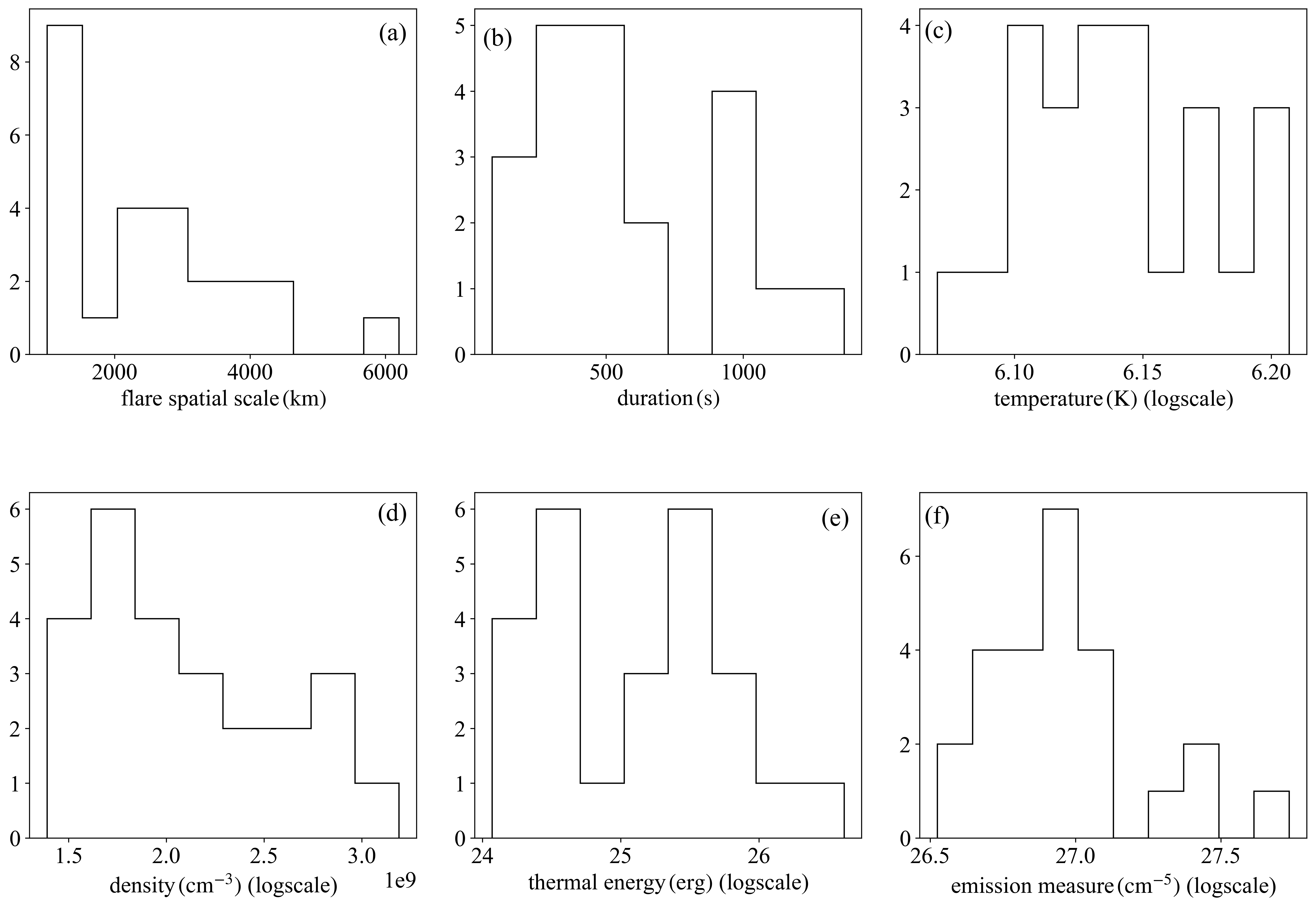
Figure 2: Histogram of the physical quantities of the events analyzed in this study. The panels (a), (c), and (f) are the same as in fig. 5 of Kotani et al. (2023).

We show the physical quantities and their histograms for the events analysed in this study in Table 1 and Fig. 2. We can see from Fig. 2 that the events have spatial scales $L$ (square root of the area of brightening pixels) between $1000\,\mathrm{km}$ and $6000\,\mathrm{km}$ and durations $t_{\mathrm{dur}}$ between $100\,\mathrm{s}$ and $1000\,\mathrm{s}$. The events have temperatures $T_{\mathrm{DEM}}$ between $10^{6.05}\,\mathrm{K}$ and $10^{6.2}\,\mathrm{K}$ and emission measure (EM) between $10^{26.5}\,\mathrm{cm}^{-5}$ and $10^{27.5}\,\mathrm{cm}^{-5}$. From these values, we can estimate the thermal energies between $10^{24}\,\mathrm{erg}$ and $10^{26.5}\,\mathrm{erg}$ and electron densities $n$ between $1.5\times 10^{9}\,\mathrm{cm}^{-3}$ and $3.0\times 10^{9}\,\mathrm{cm}^{-3}$. Note that kinetic energies of chromospheric temperature ejecta were estimated in our previous study (Kotani et al., 2023, Fig. 7). As a result, the kinetic energies tended to be greater than the thermal energies.

Based on these spatial scales and durations, we expect that the events analysed in this study correspond to the smaller events analysed in Aschwanden et al. (2000). Whilst the temperature is consistent with the results of their study, the density is a factor of three to ten times larger in our analysis. This difference in density is expected due to the different methods used to obtain the DEM. Aschwanden et al. (2000) estimated EM from the 195 Å  filter of TRACE. By contrast, we used AIA 6 channels to estimate DEM distributions for a wider range of temperatures and the sum of these was used as EM. Thus, the EM values estimated in Aschwanden et al. (2000) are typically ten times smaller than those in our analysis. The thermal energy values appear to be consistent with Aschwanden et al. (2000); however, given the different density values, they may have underestimated the thermal energy by a factor of three to ten.

By comparing the recent SO/EUI campfire observations with the current analysis, we can see that our event corresponds to a large campfire (Berghmans et al., 2021). Spatial scale, lifetime, and EM have larger values in our analysis, whilst temperature values were almost the same. All of our events occurred at the network boundary, and we could clearly see flux cancellation in 92 % of the events. These features are consistent with campfires (Berghmans et al., 2021; Panesar et al., 2021).

Some of the events analysed in this study had some distinctive qualitative characteristics. Nine of the analysed events occurred at CBPs. It is known that small flares with eruptions of cold plasma also occur in CBPs (Madjarska, 2019). We should note that the events at CBP tended to have larger temperatures and electron densities but not as large as the microflares in the active region (Hannah et al., 2008). Coronal jets were also observed in several of our events. Considering that a jet with chromospheric temperature accompanying a coronal jet is formed by magnetic forces (Yokoyama & Shibata, 1996), it is a natural result that coronal jets were observed in some of our events, which had chromospheric plasma eruptions. Some recent campfire observations have also reported the appearance of jets with coronal brightenings (Chitta et al., 2021b).

3.2 H$\alpha$ spectrum

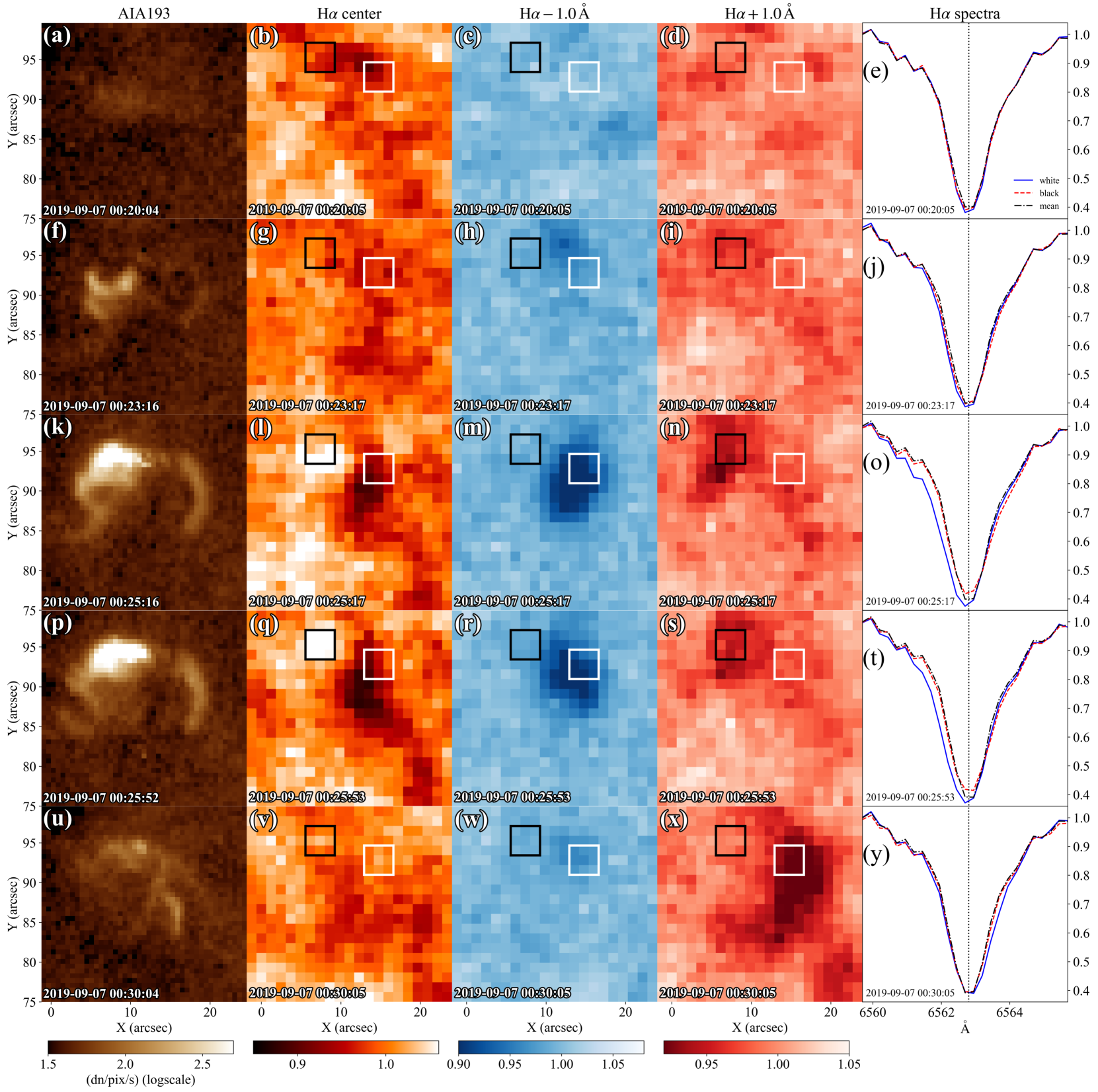
Figure 3: The time evolution of a typical event in the SDDI images and spectra. The event is the same as in Fig. 1. The left column shows the AIA 193 Å  images shown for comparison. The middle columns show the time evolution in the H$\alpha$ line at line centre, $-1.0$ Å, and $+1.0$ Å, respectively, from left to right. Each image is normalised by the average intensity of the surrounding area. Black squares indicate pixels of brightening at line centre with redshift. White squares indicate pixels of dark ejecta. The right column shows the time evolution of the H$\alpha$ spectra. The solid blue and dashed red lines indicate spectra averaged by white and black squares, respectively. The dash-dotted black line indicates the average spectra of the surrounding area. Each spectrum is normalised to the H$\alpha-3.0$ Å  intensity of the average spectrum.

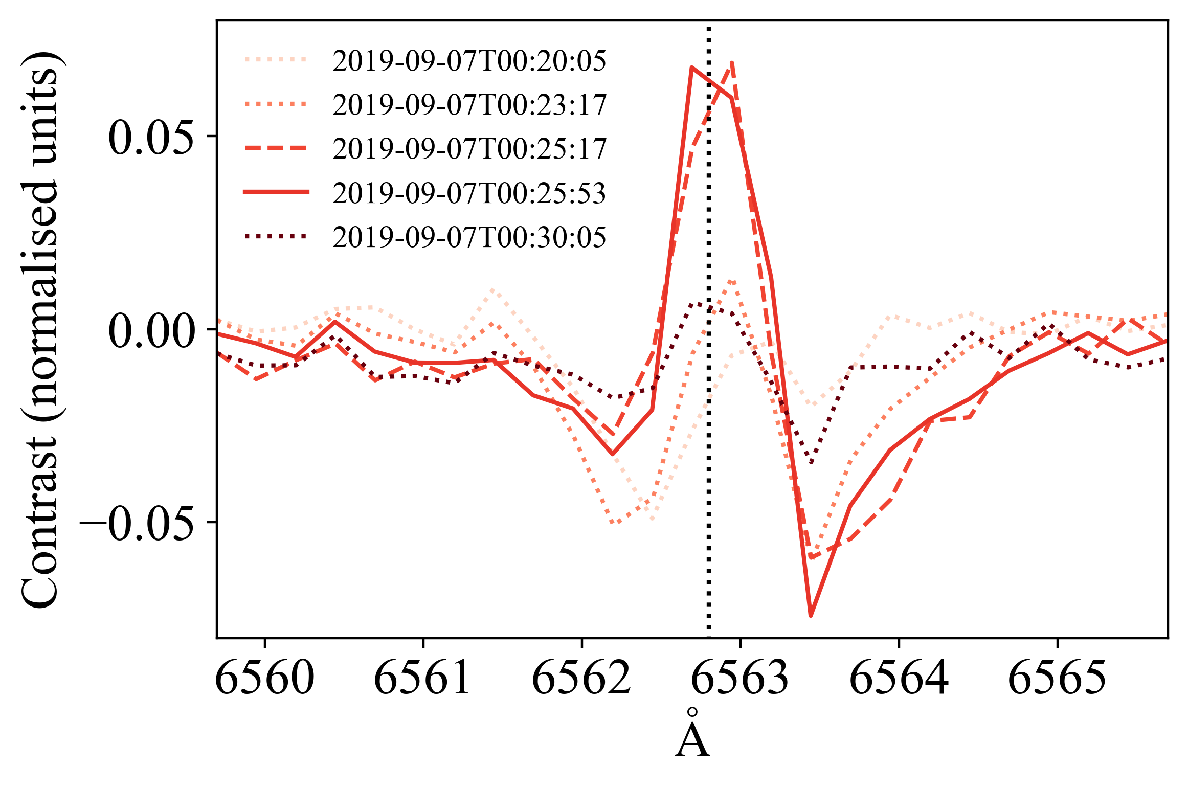
Figure 4: Time evolution of contrast for the redshift associated with the line centre brightening. Contrast is obtained as $(I_{\mathrm{red}}-I_{0})/I_{0}$, where $I_{\mathrm{red}}$ is the redshifted spectrum shown as the red line in Fig. 3 and $I_{0}$ is the average spectrum shown as the black line. Each line shows the contrast at each time of Fig.3.

In Figs. 3 and 4 we show a typical example of a small flare recorded in the AIA 193 Å  and H$\alpha$ line. We can see a brightening in the corresponding pixels in the H$\alpha$ line centre at the time when the brightness in AIA 193 Å  reaches its peak (Figs. 3l and q black squares). This enhancement is insignificant as the intensity increases by only about 5 % over the ambient intensity. This brightening is seen in the H$\alpha$ images taken at $+1.0$ Å  as a dark structure; that is, it is associated with H$\alpha$ redshift (Figs. 3n, o, s, and t). We show its characteristics more explicitly by calculating the contrast of the redshifted spectra (Fig. 4). In addition, the dark ejecta identified in the AIA images is also visible as absorption in the H$\alpha$ line centre (Figs. 3l and q white sqares). This ejecta is also seen in the H$\alpha-1.0$ Å; thus, it shows blueshifted absorption(Figs. 3m, o, r, and t). These results confirm that the dark ejecta identified in the AIA images contain plasma at chromospheric temperatures. After the brightening and blueshift disappear, another redshifted absorption appears near the pixel where the ejecta was originally in the H$\alpha+1.0$ Å  (Figs. 3x and y). Based on the spatial and temporal consistency with the ejecta observed in the blueshift, this redshift would be the ejecta falling due to gravity.

We found a redshift associated with line centre brightening in the H$\alpha$ line corresponding to AIA brightening in 14 cases. Previous studies often reported the enhancement at the line centre associated with minifilament eruption (Hermans & Martin, 1986; Sakajiri et al., 2004; Madjarska et al., 2020). However, the redshift with the line centre brightening has rarely been observed in chromospheric spectra (Kontogiannis et al., 2020; Madjarska et al., 2022; Panesar et al., 2022), and this is the first time it has been investigated in many events. This result indicates that even small flares in the QS can affect the chromosphere. The reason that the brightening and redshift were observed in only half of the events could be attributed to the insufficient spatial resolution of the SDDI. Another reason could be that the energy flux injected into the chromosphere is not extremely large compared to the radiation flux in the chromosphere. We can estimate the thermal conduction flux $F_{\mathrm{cond}}$ (in units of $\,\mathrm{erg}\,\mathrm{cm}^{-2}\,\mathrm{s}^{-1}$) using the typical physical quantities of the events analysed in this study as follows:

$$F_{\mathrm{cond}}\sim\kappa_{0}\frac{T_{\mathrm{DEM}}^{7/2}}{L}\simeq 9.0\times 10^{6}\left(\frac{T_{\mathrm{DEM}}}{10^{6.1}\,\mathrm{K}}\right)^{7/2}\left(\frac{L}{2.5\times 10^{8}\,\mathrm{cm}}\right)^{-1},$$ (1)

where $\kappa_{0}\simeq 10^{-6}\,\mathrm{cgs}$ is the Spitzer thermal conductivity. This value is larger than the energy flux in the chromosphere (upper chromosphere: $3\times 10^{5}\,\mathrm{erg}\,\mathrm{cm}^{-2}\,\mathrm{s}^{-1}$, middle chromosphere: $2\times 10^{6}\,\mathrm{erg}\,\mathrm{cm}^{-2}\,\mathrm{s}^{-1}$, Withbroe & Noyes, 1977) but much smaller than the energy flux of a typical solar flare ($>10^{9}\,\mathrm{erg}\,\mathrm{cm}^{-2}\,\mathrm{s}^{-1}$).

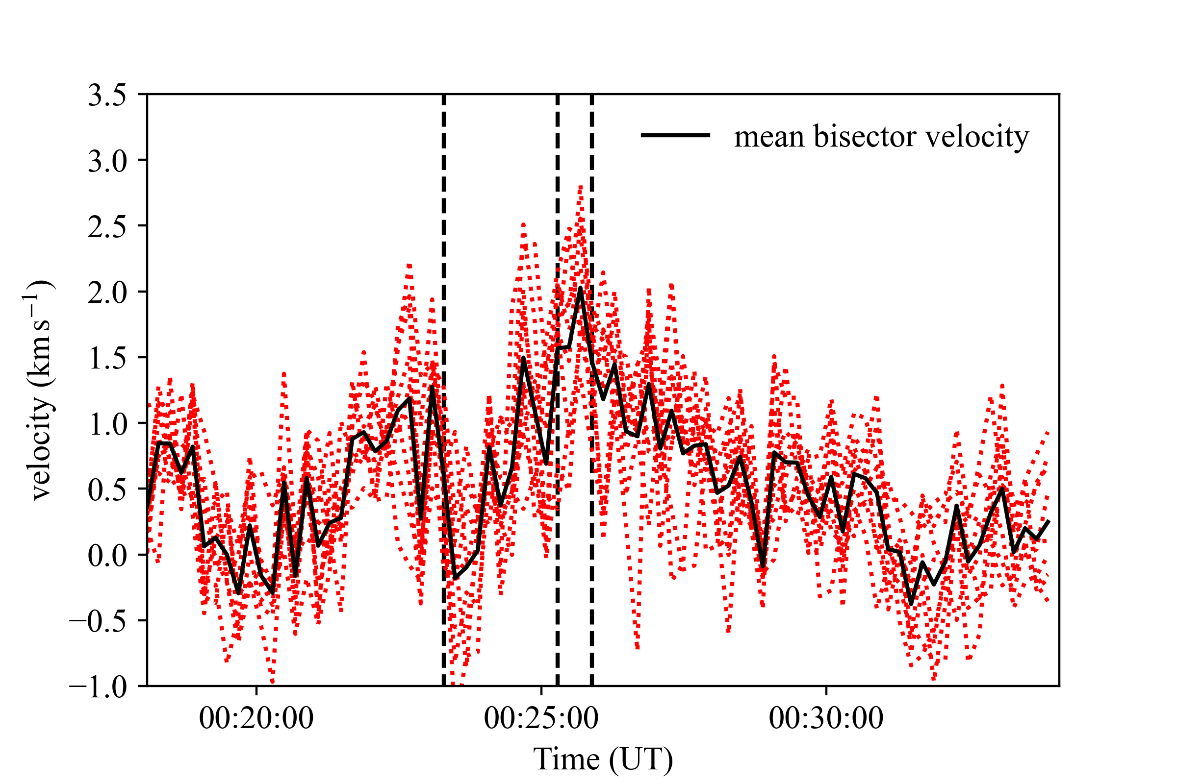
Figure 5: Typical example of redshift velocity with brightening in H$\alpha$ line centre. The event is the same as in Fig. 1. The dashed black vertical lines indicate the times in Figs. 1e, i, and m, respectively. The dotted red lines indicate the time evolution at each of the pixels surrounded by the black squares in Fig. 3. The solid black line shows the average of the dotted red lines.

We determined the bisector velocity to characterise the redshift associated with the brightening of the H$\alpha$ line centre (Kulander & Jefferies, 1966). We obtained the intensity $I_{\mathrm{bis}}$ for determining the bisector velocity as follows:

$$I_{\mathrm{bis}}=I_{\mathrm{H\alpha}}(0\,\text{\AA})+0.35\left(\frac{I_{\mathrm{H\alpha}}(+3.0\,\text{\AA})+I_{\mathrm{H\alpha}}(-3.0\,\text{\AA})}{2}-I_{\mathrm{H\alpha}}(0\,\text{\AA})\right),$$ (2)

where $I_{\mathrm{H\alpha}}(\lambda\,\text{\AA})$ is the H$\alpha$ intensity at wavelengths shifted by $\lambda$ Å  from the line centre. With the two wavelengths corresponding to the intensity $I_{\mathrm{bis}}$ as $\lambda_{+}$ and $\lambda_{-}$, we determined the bisector velocity $v_{\mathrm{red}}$ as follows:

$$v_{\mathrm{red}}=\frac{0.5(\lambda_{+}+\lambda_{-})-\lambda_{0}}{\lambda_{0}}c,$$ (3)

where $\lambda_{0}=6562.8$ Å  is the H$\alpha$ line centre wavelength and $c=3.0\times 10^{5}\,\mathrm{km}\,\mathrm{s^{-1}}$ is the light speed. The bisector velocity corresponding to the intensity $I_{\mathrm{bis}}$ was determined for each of the 9 pixels where brightening occurred, as shown in Fig. 3. We then took the average of these 9 pixels. We show the typical behaviour of the bisector velocity obtained at each time in Fig. 5. We can see from Fig. 5 that the bisector velocity increases with the brightening. We focused on the average bisector velocity of 9 pixels, and the maximum value of its time evolution was taken as the bisector velocity of the event.

We summarise the bisector velocity $v_{\mathrm{red}}$ for each event in Table 1. The events have bisector velocities between $1.0\,\mathrm{km}\,\mathrm{s}^{-1}$ and $5.0\,\mathrm{km}\,\mathrm{s}^{-1}$. These values are slightly larger than the redshift velocity in the steady chromosphere (Chae et al., 1998).

3.3 Light Curve

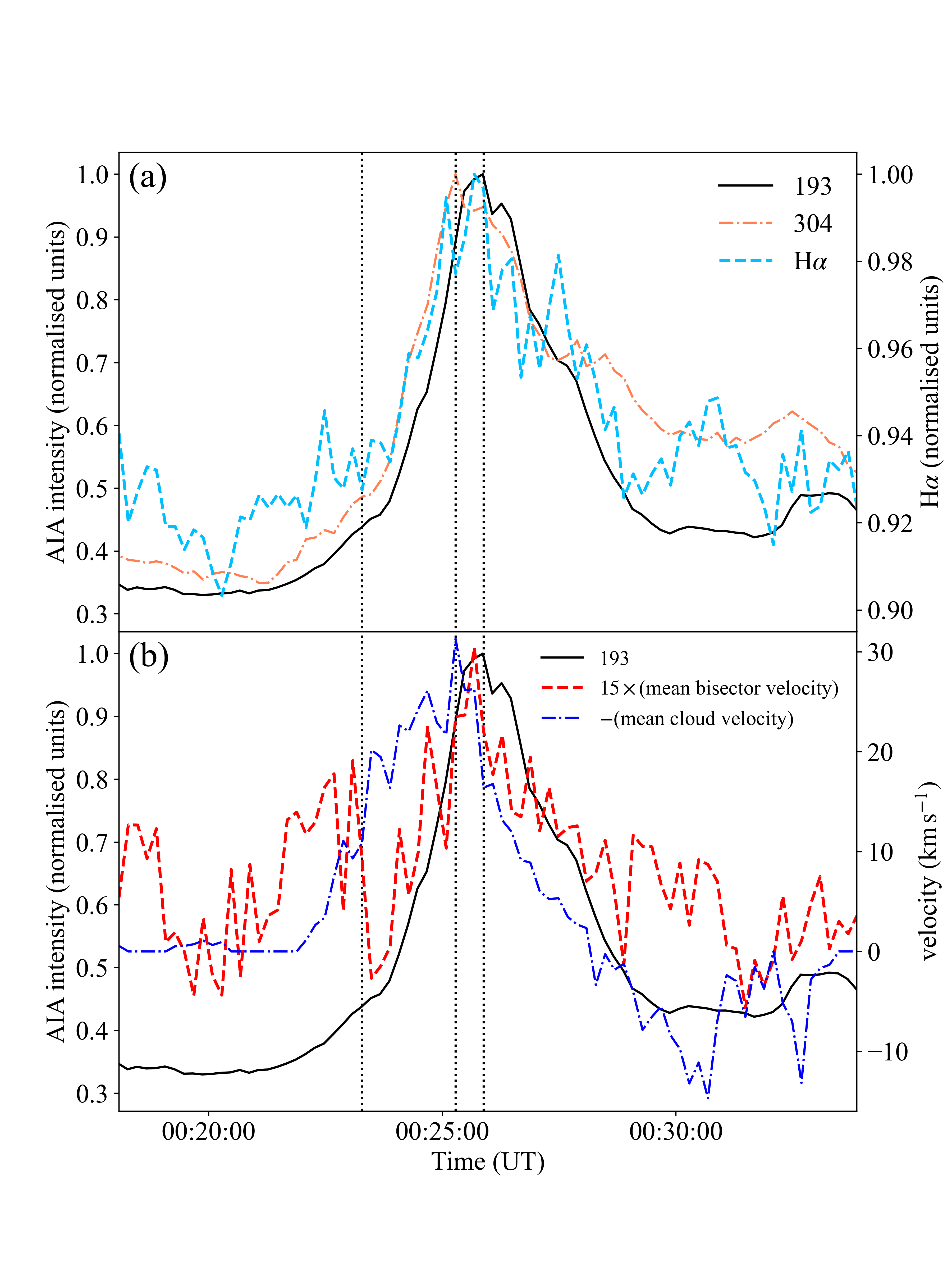
Figure 6: Typical examples of the light curves. The event is the same as in Fig. 1. The dotted black vertical lines indicate the times in Figs. 1e, i, and m, respectively. (a): AIA 193 Å and 304 Å, and H$\alpha$ line centre light curves. The solid black, dashed light blue, and dash-dotted orange lines indicate the light curves of 193 Å, 304 Å, and H$\alpha$ line centre, respectively. (b): Comparison of AIA 193 Å  light curves with redshift velocities with brightening in H$\alpha$ centre, and velocities of the dark ejecta. The dashed red and dash-dotted blue lines indicate the velocity of the redshift and the dark ejecta, respectively. The redshift velocity is shown multiplied by a factor of 15. The velocity of the dark ejecta is shown with the sign reversed. Note that the direction toward the observer is defined as a negative velocity.

In Fig. 6a we show a typical example of a light curve for the analysed events in this study. We obtain the AIA light curves as the sum of the pixels showing brightenings. The light curves are normalised to the maximum value. For the H$\alpha$ light curve, we use the sum of the intensities of the nine pixels shown in Fig. 3. The H$\alpha$ light curve is also normalised by its maximum value. We can see from Fig. 6a that H$\alpha$ and AIA 304 Å  show an earlier intensity increase than AIA 193 Å. This property is consistent with previous studies (Benz & Krucker, 1999; Jin et al., 2021; Madjarska et al., 2022) and is reminiscent of the Neupert effect (Neupert, 1968). Fig. 6a also shows that the brightening in the H$\alpha$ line varies only about 10 % over time.

Fig. 6b shows the time evolution of the redshifted velocity associated with line centre brightening $v_{\mathrm{red}}$ and the velocity of the chromospheric ejecta compared to the AIA 193 Å  light curve. We used the cloud model (Beckers, 1964; Mein & Mein, 1988) and obtained the line-of-sight velocities of the chromospheric ejecta. The cloud model is based on modelling the spectrum of a plasma blob above the background radiation field. That model estimates line-of-sight velocity $v_{l}$, the optical thickness of the blob $\tau_{0}$, source function $S$, and Doppler width $\Delta\lambda_{D}$ by fitting the contrast $C(\lambda)$ using the following equation:

$$C(\lambda)=\frac{I(\lambda)-I_{0}(\lambda)}{I_{0}(\lambda)}=\left(\frac{S}{I_{0}(\lambda)}-1\right)\left(1-e^{-\tau(\lambda)}\right),$$ (4)

$$\tau(\lambda)=\tau_{0}\exp\left(-\frac{\lambda-\frac{v_{l}}{c}\lambda_{0}}{\Delta\lambda_{D}}\right),$$ (5)

where $I(\lambda)$ is spectra of the plasma blob, $I_{0}(\lambda)$ is the background radiation, and $\lambda_{0}$ is a wavelength at the line centre. We used the average spectrum of the surroundings as $I_{0}(\lambda)$. We averaged the line-of-sight velocity over the nine pixels shown in Fig. 3 and examined its temporal evolution. Fig. 6b shows that both the ejecta and the redshifted velocity peaked before the 193 Å  light curve peak. The ejecta accelerates before the small flare reaches its peak, reaching a maximum value at the same time as the 304 Å  light curve. This property is consistent with the standard flare model in which mass ejection triggers magnetic reconnection (Ohyama & Shibata, 1998; Shibata et al., 1995). The redshift velocity is highly variable, and we cannot clearly identify an acceleration phase. However, its peak is synchronised with the H$\alpha$ line light curve. This fact provides stronger support that the redshift is accompanied by the line centre brightening.

4 discussion

4.1 Comparison of H$\alpha$ redshifted spectra and chromospheric condensation theory

Section 3.2 confirmed that H$\alpha$ line spectra show the line-centre brightening and redshift synchronised with the coronal brightening. Here we discuss the possibility that this redshift corresponds to chromospheric condensation in the small flares in the QS.

The line centre brightening and redshift of the H$\alpha$ line found in our study are reminiscent of the red asymmetry observed in large-scale flares (Ichimoto & Kurokawa, 1984). In large flare cases, released flare energy is injected into the chromosphere from the corona, resulting in chromospheric condensation (Fisher et al., 1985). The propagation of the condensation shock downward is observed as red asymmetry. The spectra found in this study are not emission lines; however, they are similar to the red asymmetry of large flares in that they show a redshift associated with line centre brightening. This difference is probably because the source function of the H$\alpha$ line increases due to energy injection from the corona even for small flares in the QS, but the resulting brightening is not large enough for the H$\alpha$ line to be observed in emission.

Some synthesised H$\alpha$ profiles corresponding to chromospheric condensation originating from a nanoflare have been reported to have a similar profile to the present observation. Bakke et al. (2022) performed numerical simulations for nanoflares in active regions and produced synthesised profiles of the H$\alpha$ line. As a result, they reproduced the H$\alpha$ line spectra, which remain absorption lines but show an increase in the line centre intensity and a redshift (see Bakke et al., 2022, fig. 7). However, their synthesised H$\alpha$ spectra also show a redshift at the line centre. This is different from our observations, which show almost no shift in the line centres and a redshift only around $+1.0$ Å. Their calculations also report a phase in which the H$\alpha$ line becomes an emission line before becoming an absorption line, but we found no H$\alpha$ emission line in our observation. One reason for these differences is that the spatial and temporal resolution of SDDI (pixel size: 1.23 arcsec/temporal resolution: 12 s) is not as good as the numerical simulations. In other words, we should observe a superposition of spectra from multiple loops, resulting in a difference from the synthetic observation calculated for a single loop. Another reason may be that Bakke et al. (2022) calculated using different parameters than the small loops in the QS. Bakke et al. (2022) synthesised the H$\alpha$ line with 1D radiative transfer and did not incorporate the 3D effects, which are essential for the formation of H$\alpha$ lines (Leenaarts et al., 2012). This may be one of the reasons why the H$\alpha$ lines do not completely agree with observations.

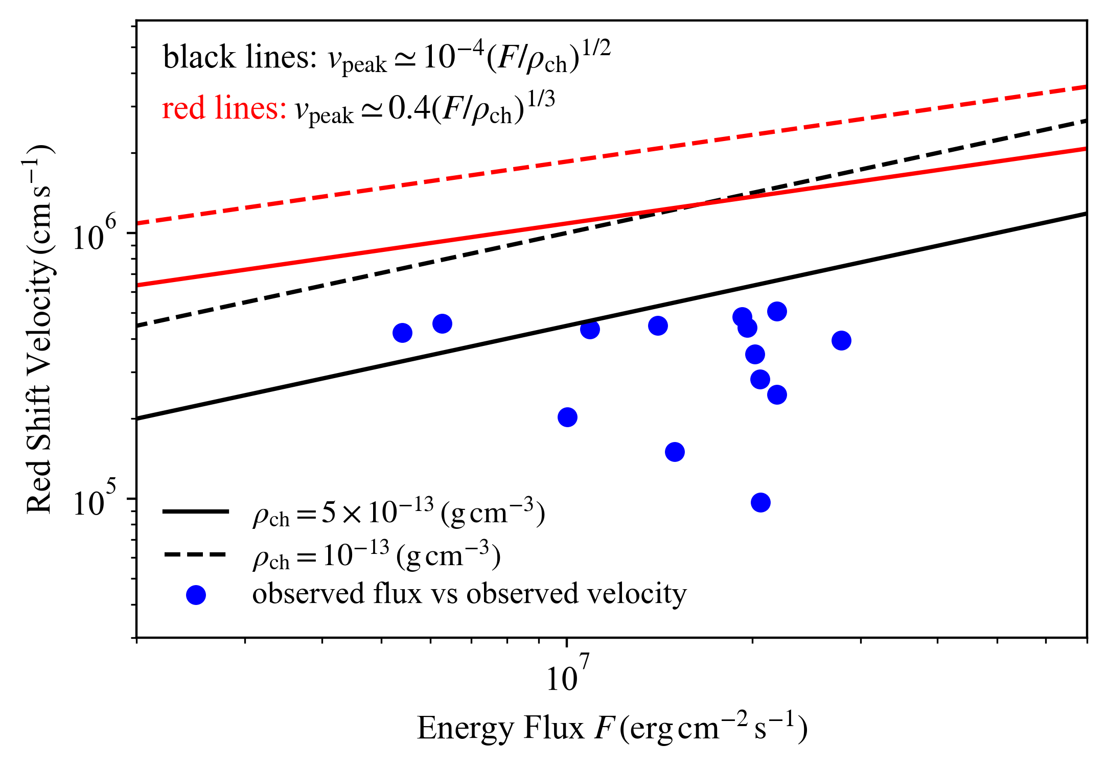
Figure 7: Comparison of the observed redshift velocity associated with brightening in the H$\alpha$ centre with the formula for chromospheric condensation (Fisher, 1989; Longcope, 2014). The black and red lines indicate the Longcope (2014) formula (equation 7) and the Fisher (1989) formula (equation 6), respectively. The solid and dashed lines show the equations (6) and (7) assuming different mass densities of the chromosphere, respectively.

We compared the observational result with the theoretical formula to verify that the observed spectra are chromospheric condensation. Following two relationships have been proposed between the maximum velocity of chromospheric condensation and the energy flux (Fisher, 1989; Longcope, 2014, in order):

$$v_{\mathrm{peak}}\simeq 0.4\left(\frac{F}{\rho_{\mathrm{ch}}}\right)^{1/3},$$ (6)

$$v_{\mathrm{peak}}\simeq 10^{-4}\left(\frac{F}{\rho_{\mathrm{ch}}}\right)^{1/2},$$ (7)

where $v_{\mathrm{peak}}$ is the condensation peak velocity (in units of $\mathrm{cm}\,\mathrm{s}^{-1}$)and $\rho_{\mathrm{ch}}$ is the pre-flare mass density in the upper chromosphere (in units of $\mathrm{g}\,\mathrm{cm^{-3}}$). $F$ is the injected energy flux into the condensation shock (in units of $\mathrm{erg}\,\mathrm{cm^{-2}}\,\mathrm{s}^{-1}$) in equation (6) and flare energy flux in equation (7). Fisher (1989) derived equation (6) in an analytical approach, whilst Longcope (2014) derived equation (7) empirically from the results of hydrodynamic simulations for a flare loop. Longcope (2014) said that the reason for the different powers in equations (6) and (7) is due to systematic variations in the fraction of the total energy flux reaching condensation shock.

Fig. 7 compares equations (6) and (7) and our observations. Here, we assume the thermal conduction fluxes (equation 1) for the energy flux $F$. We can see from Fig. 7 that equation (7) agrees with the upper bound of the observed velocities. Considering that equation (7) corresponds to the maximum condensation velocity, this result supports the interpretation that the spectral variations are due to the chromospheric condensation. In addition, the better agreement of the Longcope (2014) formula than the Fisher (1989) formula is consistent with the case of small-energy flares in the numerical simulation of Ashfield & Longcope (2021).

Another candidate for heated downflow is reconnection outflow, that is, plasma flow accelerated in a current sheet. However, it is unlikely that the observed spectral variations are due to reconnection outflows for the following two reasons. First, the observed redshift velocity is small compared to the Alfvén velocity in the chromosphere. Assuming typical parameters for the upper chromosphere, we can estimate the Alfvén velocity ($v_{A}$, in units of $\mathrm{cm}\,\mathrm{s^{-1}}$) as follows:

$$v_{A}=\frac{B_{\mathrm{ch}}}{\sqrt{4\pi\rho_{\mathrm{ch}}}}=4.0\times 10^{6}\left(\frac{B_{\mathrm{ch}}}{10\,\mathrm{G}}\right)\left(\frac{\rho_{\mathrm{ch}}}{5\times 10^{-13}\,\mathrm{g}\,\mathrm{cm^{-3}}}\right),$$ (8)

where $B_{\mathrm{ch}}$ is the magnetic field strength in the upper chromosphere (in units of $\mathrm{G}$). This value is more than ten times larger than our observation. Second, condensation downflow should be easier to observe than reconnection outflow because of its larger spatial scale. Reconnection outflow is collimated thin and stops when it collides with the lower loop. In contrast, the condensation downflow propagates along the top of the lower loop. Hence, it should have a larger spatial scale than the reconnection outflow in a typical magnetic field morphology. Based on the above discussion, although reconnection outflow may be mixed, it is likely that condensation downflow mainly contributed to the H$\alpha$ spectral variability.

4.2 Emission measure vs temperature Scaling Law

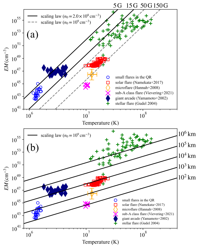
Figure 8: Comparison with EM vs temperature scaling law at time of flare peak (Shibata & Yokoyama, 1999, 2002). The blue circles indicate the analysed results of the small flares in the QS in this study. Red squares indicate typical solar flares (Namekata et al., 2017a). The orange diamonds and the pink x-marks indicate microflares (Hannah et al., 2008) and sub-A class flares (Vievering et al., 2021) in active regions, respectively. The dark blue diamonds indicate large flares in the QS (giant arcades, Yamamoto et al., 2002). Green plus signs indicate stellar flares (Güdel, 2004). (a): Comparison with the scaling law (equation 9) with the coronal magnetic field strength as a parameter. The solid black and dashed gray lines assume $n_{0}=2\times 10^{8}\,\mathrm{cm}^{-3}$ and $n_{0}=10^{9}\,\mathrm{cm}^{-3}$ for the pre-flare electron density in the corona $n_{0}$, respectively. (b): Comparison with the scaling law (equation 11) with the spatial scale as a parameter. Since in equation (11) $n_{0}$ only affects the EM by a power-law index of $2/3$, we assume $n_{0}=10^{9}\,\mathrm{cm}^{-3}$ for all lines in this figure.

To understand the physical mechanism of small flares in the QS, we compared the present DEM analysis results with Shibata & Yokoyama (1999, 2002) scaling law. Shibata & Yokoyama (1999, 2002) derived the following scaling law between the volume emission measure $EM_{v}$ ($\mathrm{cm}^{-3}$) and temperature in the flare peak times:

$$EM_{v}\simeq 10^{48}\left(\frac{B_{\mathrm{corona}}}{50\,\mathrm{G}}\right)^{-5}\left(\frac{n_{0}}{10^{9}\,\mathrm{cm}^{-3}}\right)^{3/2}\left(\frac{T_{\mathrm{peak}}}{10^{7}\,\mathrm{K}}\right)^{17/2},$$ (9)

where $B_{\mathrm{corona}}$ is the coronal magnetic field strength, $n_{0}$ is the preflare electron number density, and $T_{\mathrm{peak}}$ is the temperature in the flare peak time. This scaling law is consistent with a wide range of energies, from microflares in active regions to giant stellar flares.

Fig. 8 shows the comparison of our analysis result with the scaling law of Shibata & Yokoyama (1999, 2002). Here, the volume emission measure $EM_{v}$ is calculated from the observations as follows:

$$EM_{v}=EM\times L^{2}$$ (10)

We can see from Fig. 8a that the present observation agrees with the case where $B_{\mathrm{corona}}=5-15\,\mathrm{G}$ and $n_{0}=2\times 10^{8}\,\mathrm{cm}^{-3}$ in equation (9). We also include in Fig. 8 observations of giant arcades (Yamamoto et al., 2002) for further understanding. The giant arcades are also located away from the group of active region flares and agree with equation (9) for $B_{\mathrm{corona}}=5-15\,\mathrm{G}$ and $n_{0}=2\times 10^{8}\,\mathrm{cm}^{-3}$. These results indicate that Shibata & Yokoyama (1999, 2002) scaling law can explain small flares in the QS and giant arcades by considering appropriate values of the magnetic field strength and coronal electron density in the QS.

Shibata & Yokoyama (1999, 2002) also derived the scaling law using the spatial scale $L$ rather than the magnetic field $B_{\mathrm{corona}}$ as a parameter.

$$EM_{v}\simeq 10^{48}\left(\frac{L}{10^{9}\,\mathrm{cm}}\right)^{5/3}\left(\frac{n_{0}}{10^{9}\,\mathrm{cm}^{-3}}\right)^{2/3}\left(\frac{T_{\mathrm{peak}}}{10^{7}\,\mathrm{K}}\right)^{8/3}.$$ (11)

We show in Fig. 8b our analysis results and equation (11). We can see a good agreement with the case where $L\simeq 10^{3}\,\mathrm{km}$. We can also see that some of the small flares in the QS are consistent with equation (11) for the case smaller than $1000\,\mathrm{km}$. These spatial scales are less than the thickness of the chromosphere, which may seem to be a contradictory result. However, we suggest that these spatial scales reflect that only a portion of the loops brightens at coronal temperatures. This hypothesis is consistent with recent "campfire” studies (Berghmans et al., 2021; Zhukov et al., 2021).

Aschwanden et al. (2008) also compared the $EM_{v}$ and temperature of small flares in the QS with active region flares. They obtained the following relationship by a linear regression fit for various scale solar flares:

$$EM_{v}\simeq 10^{48.4}\left(\frac{T_{\mathrm{peak}}}{10^{7}\,\mathrm{K}}\right)^{4.7\pm 0.1}.$$ (12)

The power-law index in this equation differs from those in equations (9) and (11). The following two reasons can explain this difference. First, Aschwanden et al. (2008) performed the fit without including sub-A class flares in active regions and giant arcades. Equation (12) is clearly inconsistent with these events shown in Fig. 8. The second reason is that the fitting in Aschwanden et al. (2008) did not consider differences in the physical quantities associated with flares. They performed the fitting simultaneously for flares in quiet and active regions where the magnetic field strength differs. The difference in the magnetic field strength affects the Poynting flux that heats the atmosphere associated with the flare, causing differences in the temperature for the same EM. Hence, the power index should be smaller than the value in equation (9) ($=17/2$). From the above discussion, we can say that equation (12) is the result of fitting by focusing on only some of the many flares that occur in the solar atmosphere without considering the differences in their parameters. Therefore, it would not be easy to obtain a unified view of flares based on this formula.

We can expect from Fig. 8 that the following assumptions of Shibata & Yokoyama’s scaling law hold even for small flares in the QS.

1. Cooling by thermal conduction and heating by magnetic reconnection are balanced.

   $$\kappa_{0}\frac{T_{\mathrm{max}}^{7/2}}{2L^{2}}\simeq\frac{B_{\mathrm{corona}}^{2}}{4\pi}\frac{v_{A}}{L},$$ (13)

   where $\kappa_{0}\simeq 10^{-6}\,\mathrm{cgs}$ is the Spitzer thermal conductivity, $T_{\mathrm{max}}$ is the maximum temperature in the flare, and $v_{A}$ is the Alfvén velocity.

2. The maximum flare temperature $T_{\mathrm{max}}$ is three times higher than the temperature observed at the flare peak time $T_{\mathrm{peak}}$.

3. The high-temperature, high-density plasma originating from the chromosphere is the origin of the brightening in the corona.

   $$EM_{v}\simeq n^{2}L^{3},$$ (14)

   where $n$ is the increased flare-loop density.

4. The magnetic pressure of the loop confines the high-temperature, high-density plasma originating from the chromosphere.

   $$2nk_{B}T_{\mathrm{peak}}\simeq\frac{B_{\mathrm{corona}}^{2}}{8\pi},$$ (15)

   where $k_{B}$ is the Boltzmann constant.

The fact that small flares in the QS also show these properties is essential for understanding the physical mechanism of nanoflares.

4.3 Time evolution of flare temperature and density

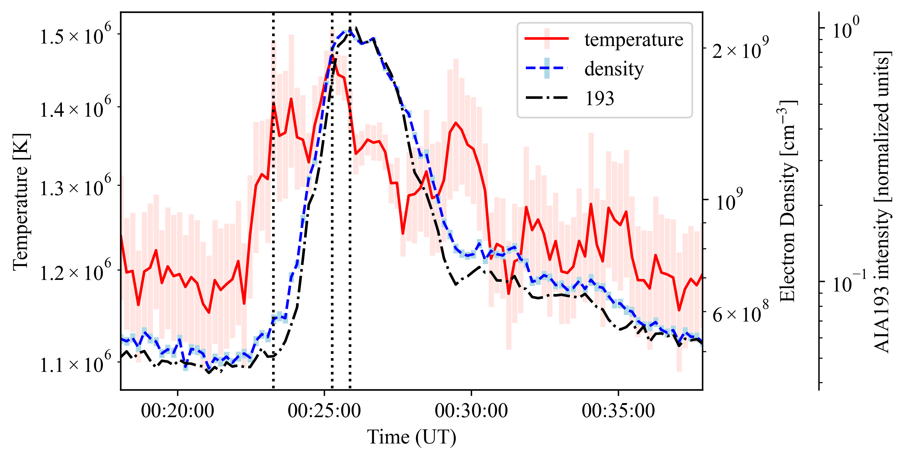
Figure 9: Typical example of the time evolution of density and temperature of a small flare. The event is the same as in Fig. 1. The dotted black vertical lines indicate the times in Figs. 1e, i, and m, respectively. The solid red, dashed blue, and dash-dotted black lines show the time evolution of the temperature, density, and 193 Å  intensity, respectively. Error bars of the temperature and density calculations are from the errors in estimating the DEM.

We investigated the time evolutions of temperature and density to understand how heating from small reconnection in the QS affects the atmosphere. The time evolution of flare temperature and density has been well studied in large solar flares by numerical simulations and observations (e.g., Nagai, 1980; Serio et al., 1991; Jakimiec et al., 1992; Sylwester et al., 1993; Shibata & Yokoyama, 2002). Reale (2007, 2014) summarised the time evolution of flare temperatures and densities in the following four phases (see Reale, 2007, fig.1. and 2.).

1. From the start of the heat pulse to the temperature peak (heating).

2. From the temperature peak to the end of the heat pulse (evaporation).

3. From the end of the heat pulse to the density peak (conductive cooling).

4. From the density peak afterwards (radiative cooling).

We averaged the temperature and density at $3\times 3$ pixels to investigate the time evolution. To select pixels for the time evolution of temperature and density, we referred to the time when the AIA 193 Å  light curve was at its maximum. At that time, we defined the $3\times 3$ pixels, centred on the pixel with the largest AIA 193 Å  intensity. We have fixed and limited the analysed pixels to facilitate comparison with the time evolution of the single-loop model (e.g., Jakimiec et al., 1992).

Fig. 9 shows a typical example of the time evolution of the density and temperature. We can see from Fig. 9 that the temperature increase precedes the density increase. The density and AIA 193 Å  light curves reach their peaks almost simultaneously after the temperature peaks. After the density peak, it decays a little more slowly than the AIA 193 Å  light curve. The qualitative characteristics of these time evolutions are the same as those of large-scale flares (Reale, 2007, 2014). The result that the temperature increase precedes the density increase suggests that chromospheric evaporation occurs even in small flares in the QS. We found 15 events in which the temperature peak preceded the density peak. This trend is consistent with the analysis of Benz & Krucker (1998).

We note that the density increase simultaneously with coronal intensity increase was also found by Kamio et al. (2011), who described it as supporting chromospheric evaporation models. However, only the fact that the density increase is synchronised with the coronal brightening is not enough to indicate the presence of chromospheric evaporation. This is because optically thin coronal plasmas are sensitive to density fluctuations. Moreover, numerical simulations suggest that the shocks also cause fluctuations in physical quantities comparable to those of nanoflares (Moriyasu et al., 2004; Antolin et al., 2008). The preceding temperature increase than the density increase more strongly supports the scenario that reconnection occurs in the corona and the released energy propagates to the chromosphere, resulting in evaporation.

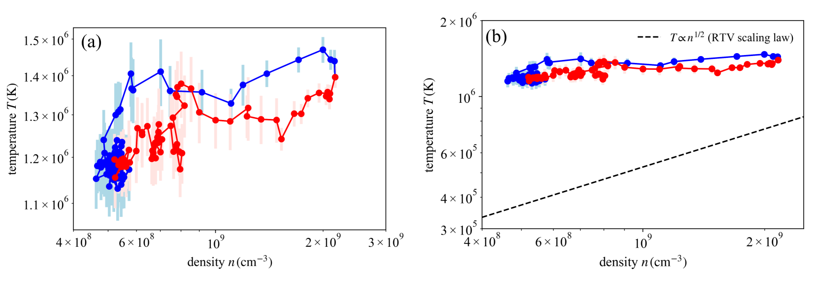
Figure 10: Typical example of the temperature-density (T-N) diagram. The event is the same as in Fig. 1. (a): T-N diagram shown in large size. (b): Comparison with RTV scaling law (equation 16, Rosner et al., 1978). The dashed black line is the RTV scaling law calculated at the spatial scale of event 4 in Table 1.

Fig. 10 shows a typical temperature-density (T-N) diagram for small flares in the QS. From Fig. 10a, we can see that the temperature and density increase process is qualitatively the same as for large flares (Reale, 2007, 2014). In contrast, Fig. 10b shows that the temperature is about three times higher than that determined by the RTV scaling law (Rosner et al., 1978) in the pre and post-flare phases. The power-law index of the decay phase is gradual and almost constant.

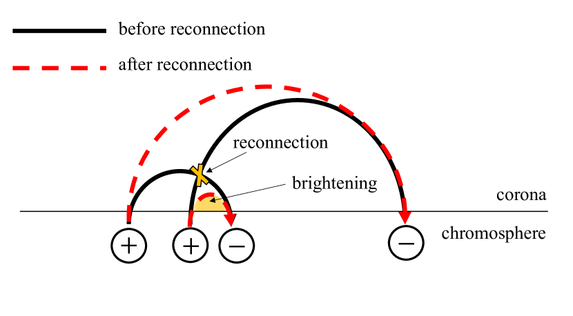
Figure 11: Schematic diagram showing an example of a magnetic field morphology that can underestimate the spatial scale.

There are multiple reasons for the higher temperatures than expected from the RTV scaling law, even without the occurrence of small flares. The first is the possibility that small loops in the QS are not in a steady state. The second possibility is that the spatial scale determined from the brightening pixels underestimates the actual loop length since brightening is seen only in part of the loop. These underestimations will appear as a brightening only near the top of the loop (Berghmans et al., 2021; Zhukov et al., 2021). Also, if the brightening of a small loop formed by reconnection is observed primarily, as in Fig. 11, the spatial scale will be underestimated. Then the question to ask is: how much underestimation of the actual loop length would make the temperature consistent with the RTV scaling law when the flare is not occurring? The RTV scaling law for the relationship between temperature and density is as follows:

$$T=4.3\times 10^{5}\left(\frac{n}{10^{9}\,\mathrm{cm}^{-3}}\right)^{1/2}\left(\frac{L}{2.5\times 10^{8}\,\mathrm{cm}}\right)^{1/2}.$$ (16)

Therefore, the spatial scale must be underestimated by approximately one order of magnitude.

A third possibility is that the DEM analysis using AIA itself was problematic. The temperature response functions of the six AIA channels used in the DEM analysis have no peak around $10^{5.5}\sim 3.2\times 10^{5}\,\mathrm{K}$ (Landi et al., 2013). The smallest temperature peak is about $10^{5.8}\sim 6.3\times 10^{5}\,\mathrm{K}$ in AIA 131 Å, which is higher than the temperature of $4.3\times 10^{5}\sim 10^{5.63}\,\mathrm{K}$ expected from the RTV. Therefore, the AIA DEM analysis may not be able to diagnose plasmas that is at a temperature as low as $10^{5.5}\,\mathrm{K}$. We believe that the AIA DEM analysis may be the most influential in the above three possibilities since the temperature in the absence of flares is about $10^{6}\,\mathrm{K}$ for all events. Hence, the temperatures when flares are not occurring and during the decay phase will need to be investigated differently.

Although one may speculate that the temperature diagnostics problem identified by the DEM analysis above could extend to the flare peak time, as illustrated in Fig. 8, we anticipate that the results of DEM analysis by AIA are reliable in the vicinity of the flare peak time. If the primary component of the flare is low-temperature ($\sim 10^{5}\,\mathrm{K}$) plasma that is not detectable by DEM analysis, magnetic reconnection is likely to occur in or below the transition region. This is because, according to the AIA temperature response function, low-temperature plasmas must have a high density ($\sim 10^{10}\,\mathrm{cm^{-3}}$) to account for the observed small brightenings (Dolliou et al., 2023). However, our investigation revealed evidence of reconnection occurring above the transition region in more than half of the events, as demonstrated by the temporal variations in physical quantities (Fig. 9) and light curves (Fig. 6). Thus, we expect most of the events examined in this study to have temperatures exceeding ($\sim 10^{5}\,\mathrm{K}$) around the flare peak time.

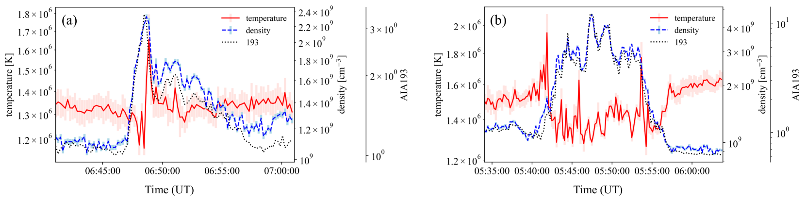
Figure 12: Examples of the temperature and density evolution that differ from typical events.

We present two examples of temperature and density temporal evolution showing peculiar behaviour. The first example is events in which the density peak precedes the temperature peak (Fig. 12a). We identified five such examples. One of the causes of these events is the failure to fully resolve the single loop. In other words, the temperature increase corresponding to the density peak may not have been captured by the selected pixels. In such cases, we may capture the temperature increase corresponding to the small brightenings that repeatedly occur after the density peak. Another possibility is that reconnection below the transition region heated the dense plasma to coronal temperatures (Chen et al., 2021). Since the AIA DEM analysis basically describes plasma at coronal temperatures, the observed EM value should increase when plasma at chromospheric/transition region temperatures is heated to coronal temperatures. In such cases, the plasma in the chromosphere/transition region should be heated to coronal temperatures with decreasing density due to expansion. Thus, the observed temperature should peak at or slightly after the density peak.

The second example is that the temperature decreases at the density peak with respect to the pre-flare one (Fig. 12b). We identified four such examples. These events occurred at CBPs and had relatively high temperatures ($T\sim 1.5\times 10^{6}\,\mathrm{K}$) before the flares occurred. Therefore, the low temperature ($T\sim 1.2\times 10^{6}\,\mathrm{K}$) plasma is considered to have increased due to chromospheric evaporation, resulting in a decrease in temperature at the density peak. We need to test this hypothesis in the future, including the perspective of what determines the temperature of chromospheric evaporation.

5 SUMMARY AND FUTURE WORK

This paper presents our analysis of many small flares in the QS using SDO/AIA and SMART/SDDI observational data, with particular attention to their thermal properties. Our analysis confirmed that the events had physical quantities that were quantitatively consistent with previous studies. We also confirmed common qualitative properties, such as that they occurred at network boundaries and that most of them were accompanied by flux cancellation. The main results of this paper are as follows:

1. Redshift with brightening of the H$\alpha$ line centre was observed in more than half of the events. These redshifts corresponded well to brightenings in the corona both temporally and spatially and were also consistent with the chromospheric condensation formula (Longcope, 2014). Therefore, they are considered to correspond to chromospheric condensation for small flares in the QS (Sections 3.2, 3.3, and 4.1).

2. The observed relationship between EM and temperature is consistent with the scaling law (Shibata & Yokoyama, 1999, 2002) for coronal magnetic field strengths of 5–15 G. This consistency suggests that the primary cooling mechanism at the flare peak time is thermal conduction and that the plasma originated from the chromosphere through evaporation significantly affects the brightening. In other words, it suggests that small flares in the QS also have qualitatively the same thermal properties in their peak time, only with reduced magnetic field and spatial scale (Section 4.2).

3. In more than half of the events, the temperature reached a maximum before the density. This result supports the idea that chromospheric evaporation occurs even in some small flares in the QS (Section 4.3).

4. Our temperature-density diagram shows that the thermal evolution of small flares always proceeds at higher temperatures than the RTV scaling law (Rosner et al., 1978). One of the reasons for this evolution at high temperatures is the possibility that we overestimate the temperatures in the steady state and decay phase due to the limitation of the observed temperature range by AIA (Section 4.3).

These results suggest that the interaction with the chromosphere may play an essential role in the thermal evolution of some small flares in the QS. This property may be the new commonality between small flares in the QS and typical active region flares. However, due to the lack of sample size and spatial resolution, our observations do not accurately answer the question of how many small flares in the QS interact with the chromosphere. Our observations also may not have captured the entire thermal evolution of the small flare in the QS. To solve these problems, simultaneous higher spatial resolution spectroscopic observations of the chromosphere (e.g., with SST/CRISP or DKIST/VTF) and observations capable of diagnosing temperatures from $10^{4}$ to $10^{6}\,\mathrm{K}$ with equally high spatial and temporal resolution (e.g., IRIS or Solar-C/EUVST) will be necessary.

We propose some suggestions based on our results in determining the relationship between the frequency and energy of small flares in the QS. To determine the power-law index of the relationship, we need a proper detection method and method for determining flare energy over a wide energy range. Regarding the flare detection method, our study suggests that using coronal intensity and EM fluctuations as detection criteria might be ineffective in identifying heating events with slight intensity variations. This is because the density and intensity of the corona showed similar time evolution in our analysis, but the temperature behaved differently from them (Figs 9 and 12). In other words, density rather than temperature provides the major contribution to the coronal intensity. These heating events with slight intensity variations would correspond to QS versions of the heating events without X-ray brightening observed in active regions (Ishikawa et al., 2017). Potential instances of heating events characterised by minimal density fluctuations could include scenarios where magnetic reconnection occurs, yet the energy transported into the chromosphere remains insufficient to trigger chromospheric evaporation. Such circumstances may arise when the magnetic field strength is exceptionally weak or when reconnection occurs on tiny spatial scales, as in braiding (Parker, 1988; Antolin et al., 2021). Moreover, density variations might be negligible if reconnection occurs within a high-density loop already experiencing evaporation. This situation can be rephrased as one where the reconnection cadence is shorter than the plasma cooling time (Joulin et al., 2016). If these events were to occur, how to detect heating (reconnection) events would need to be carefully verified, including numerical verification.

To determine the flare energy, we propose estimating the radiation energy in the chromosphere of a small flare in the QS. The energy partition of flares, including large flares, is an open question. In particular, Warmuth & Mann (2020) has proposed that thermal-nonthermal energy partition changes with flare energy. Hence, using thermal energy as the flare energy may be an inappropriate definition for comparing flares with a wide range of energies. On the other hand, the bolometric radiated energy is considered a good proxy for the dissipated magnetic energy of the flare. The bolometric energy is estimated from variations in the total solar irradiance (TSI) (Kretzschmar, 2011; Emslie et al., 2012), with the main contribution coming from visible and UV wavelengths. It would be impossible to estimate the bolometric energy from TSI variations for small flares in the QS; however, it is possible to estimate the radiative energy of the chromosphere from non-LTE inversion (Yadav et al., 2022). By estimating the radiative energy of the chromosphere for small flares, the flare energy can be defined more accurately, which may help solve the coronal heating problem.

DATA AVAILABILITY

The SDO/AIA and SDO/HMI data underlying this article are available in http://jsoc.stanford.edu/ajax/lookdata.html. SMART/SDDI data are available at https://www.hida.kyoto-u.ac.jp/SMART/daily/19Sep/daily/images_20190907.html for some wavelengths. All wavelength data for SMART/SDDI can be obtained by requesting data_info@kwasan.kyoto-u.ac.jp. The derived data generated in this work will be shared on reasonable request to the corresponding author.

References

- Antolin et al. (2008) Antolin P., Shibata K., Kudoh T., Shiota D., Brooks D., 2008, ApJ, 688, 669
- Antolin et al. (2021) Antolin P., Pagano P., Testa P., Petralia A., Reale F., 2021, Nature Astronomy, 5, 54
- Aschwanden (2020) Aschwanden M. J., 2020, ApJ, 903, 23
- Aschwanden et al. (2000) Aschwanden M. J., Tarbell T. D., Nightingale R. W., Schrijver C. J., Title A., Kankelborg C. C., Martens P., Warren H. P., 2000, ApJ, 535, 1047
- Aschwanden et al. (2008) Aschwanden M. J., Stern R. A., Güdel M., 2008, ApJ, 672, 659
- Ashfield & Longcope (2021) Ashfield W. H., Longcope D. W., 2021, ApJ, 912, 25
- Bakke et al. (2022) Bakke H., Carlsson M., Rouppe van der Voort L., Gudiksen B. V., Polito V., Testa P., De Pontieu B., 2022, A&A, 659, A186
- Barnes et al. (2020) Barnes W. T., et al., 2020, Journal of Open Source Software, 5, 2801
- Beckers (1964) Beckers J. M., 1964, PhD thesis, Sacramento Peak Observatory, Air Force Cambridge Research Laboratories, Mass., USA
- Benz & Krucker (1998) Benz A. O., Krucker S., 1998, Sol. Phys., 182, 349
- Benz & Krucker (1999) Benz A. O., Krucker S., 1999, A&A, 341, 286
- Benz & Krucker (2002) Benz A. O., Krucker S., 2002, ApJ, 568, 413
- Berghmans et al. (1998) Berghmans D., Clette F., Moses D., 1998, A&A, 336, 1039
- Berghmans et al. (2021) Berghmans D., et al., 2021, A&A, 656, L4
- Canfield et al. (1990) Canfield R. C., Penn M. J., Wulser J.-P., Kiplinger A. L., 1990, ApJ, 363, 318
- Chae et al. (1998) Chae J., Yun H. S., Poland A. I., 1998, ApJS, 114, 151
- Chen et al. (2021) Chen Y., Przybylski D., Peter H., Tian H., Auchère F., Berghmans D., 2021, A&A, 656, L7
- Chitta et al. (2021a) Chitta L. P., Peter H., Young P. R., 2021a, A&A, 647, A159
- Chitta et al. (2021b) Chitta L. P., et al., 2021b, A&A, 656, L13
- Dolliou et al. (2023) Dolliou A., et al., 2023, A&A, 671, A64
- Emslie et al. (2012) Emslie A. G., et al., 2012, ApJ, 759, 71
- Fisher (1989) Fisher G. H., 1989, ApJ, 346, 1019
- Fisher et al. (1985) Fisher G. H., Canfield R. C., McClymont A. N., 1985, ApJ, 289, 434
- Galsgaard et al. (2019) Galsgaard K., Madjarska M. S., Mackay D. H., Mou C., 2019, A&A, 623, A78
- Güdel (2004) Güdel M., 2004, A&ARv, 12, 71
- Hannah & Kontar (2012) Hannah I. G., Kontar E. P., 2012, A&A, 539, A146
- Hannah et al. (2008) Hannah I. G., Christe S., Krucker S., Hurford G. J., Hudson H. S., Lin R. P., 2008, ApJ, 677, 704
- Hermans & Martin (1986) Hermans L. M., Martin S. F., 1986, in NASA Conference Publication. pp 369–375
- Hudson (1991) Hudson H. S., 1991, Sol. Phys., 133, 357
- Ichimoto & Kurokawa (1984) Ichimoto K., Kurokawa H., 1984, Sol. Phys., 93, 105
- Ichimoto et al. (2017) Ichimoto K., et al., 2017, Sol. Phys., 292, 63
- Inoue et al. (2014) Inoue S., Hayashi K., Magara T., Choe G. S., Park Y. D., 2014, ApJ, 788, 182
- Ishikawa et al. (2017) Ishikawa S.-n., Glesener L., Krucker S., Christe S., Buitrago-Casas J. C., Narukage N., Vievering J., 2017, Nature Astronomy, 1, 771
- Jakimiec et al. (1992) Jakimiec J., Sylwester B., Sylwester J., Serio S., Peres G., Reale F., 1992, A&A, 253, 269
- Jiang et al. (2013) Jiang C., Feng X., Wu S. T., Hu Q., 2013, ApJ, 771, L30
- Jin et al. (2021) Jin C. L., Zhou G. P., Wang J. X., 2021, ApJ, 914, L35
- Joulin et al. (2016) Joulin V., Buchlin E., Solomon J., Guennou C., 2016, A&A, 591, A148
- Kamio et al. (2011) Kamio S., Curdt W., Teriaca L., Innes D. E., 2011, A&A, 529, A21
- Kontogiannis et al. (2020) Kontogiannis I., Dineva E., Diercke A., Verma M., Kuckein C., Balthasar H., Denker C., 2020, ApJ, 898, 144
- Kotani et al. (2023) Kotani Y., Shibata K., Ishii T. T., Yamasaki D., Otsuji K., Ichimoto K., Asai A., 2023, ApJ, 943, 143
- Kretzschmar (2011) Kretzschmar M., 2011, A&A, 530, A84
- Krucker & Benz (1998) Krucker S., Benz A. O., 1998, ApJ, 501, L213
- Krucker et al. (1997) Krucker S., Benz A. O., Bastian T. S., Acton L. W., 1997, ApJ, 488, 499
- Kulander & Jefferies (1966) Kulander J. L., Jefferies J. T., 1966, ApJ, 146, 194
- Labonte (1979) Labonte B. J., 1979, Sol. Phys., 61, 283
- Landi et al. (2013) Landi E., Young P. R., Dere K. P., Del Zanna G., Mason H. E., 2013, ApJ, 763, 86
- Leenaarts et al. (2012) Leenaarts J., Carlsson M., Rouppe van der Voort L., 2012, ApJ, 749, 136
- Lemen et al. (2012) Lemen J. R., et al., 2012, Sol. Phys., 275, 17
- Longcope (2014) Longcope D. W., 2014, ApJ, 795, 10
- Madjarska (2019) Madjarska M. S., 2019, Living Reviews in Solar Physics, 16, 2
- Madjarska et al. (2020) Madjarska M. S., Galsgaard K., Mackay D. H., Koleva K., Dechev M., 2020, A&A, 643, A19
- Madjarska et al. (2022) Madjarska M. S., Mackay D. H., Galsgaard K., Wiegelmann T., Xie H., 2022, A&A, 660, A45
- Mein & Mein (1988) Mein P., Mein N., 1988, A&A, 203, 162
- Moore et al. (1977) Moore R. L., Tang F., Bohlin J. D., Golub L., 1977, ApJ, 218, 286
- Moriyasu et al. (2004) Moriyasu S., Kudoh T., Yokoyama T., Shibata K., 2004, ApJ, 601, L107
- Müller et al. (2020) Müller D., et al., 2020, A&A, 642, A1
- Nagai (1980) Nagai F., 1980, Sol. Phys., 68, 351
- Namekata et al. (2017a) Namekata K., Sakaue T., Watanabe K., Asai A., Shibata K., 2017a, PASJ, 69, 7
- Namekata et al. (2017b) Namekata K., et al., 2017b, ApJ, 851, 91
- Neupert (1968) Neupert W. M., 1968, ApJ, 153, L59
- Ohyama & Shibata (1998) Ohyama M., Shibata K., 1998, ApJ, 499, 934
- Panesar et al. (2021) Panesar N. K., Tiwari S. K., Berghmans D., Cheung M. C. M., Müller D., Auchere F., Zhukov A., 2021, ApJ, 921, L20
- Panesar et al. (2022) Panesar N. K., Tiwari S. K., Moore R. L., Sterling A. C., De Pontieu B., 2022, ApJ, 939, 25
- Panesar et al. (2023) Panesar N. K., Hansteen V. H., Tiwari S. K., Cheung M. C. M., Berghmans D., Müller D., 2023, ApJ, 943, 24
- Parker (1988) Parker E. N., 1988, ApJ, 330, 474
- Parnell & Jupp (2000) Parnell C. E., Jupp P. E., 2000, ApJ, 529, 554
- Pesnell et al. (2012) Pesnell W. D., Thompson B. J., Chamberlin P. C., 2012, Sol. Phys., 275, 3
- Purkhart & Veronig (2022) Purkhart S., Veronig A. M., 2022, A&A, 661, A149
- Reale (2007) Reale F., 2007, A&A, 471, 271
- Reale (2014) Reale F., 2014, Living Reviews in Solar Physics, 11, 4
- Ren et al. (2008) Ren D. B., Jiang Y. C., Yang J. Y., Zheng R. S., Bi Y., Wang M., 2008, Ap&SS, 318, 141
- Rochus et al. (2020) Rochus P., et al., 2020, A&A, 642, A8
- Rosner et al. (1978) Rosner R., Tucker W. H., Vaiana G. S., 1978, ApJ, 220, 643
- Sakajiri et al. (2004) Sakajiri T., et al., 2004, ApJ, 616, 578
- Scherrer et al. (2012) Scherrer P. H., et al., 2012, Sol. Phys., 275, 207
- Serio et al. (1991) Serio S., Reale F., Jakimiec J., Sylwester B., Sylwester J., 1991, A&A, 241, 197
- Shibata & Yokoyama (1999) Shibata K., Yokoyama T., 1999, ApJ, 526, L49
- Shibata & Yokoyama (2002) Shibata K., Yokoyama T., 2002, ApJ, 577, 422
- Shibata et al. (1995) Shibata K., Masuda S., Shimojo M., Hara H., Yokoyama T., Tsuneta S., Kosugi T., Ogawara Y., 1995, ApJ, 451, L83
- Sterling et al. (2015) Sterling A. C., Moore R. L., Falconer D. A., Adams M., 2015, Nature, 523, 437
- Sylwester et al. (1993) Sylwester B., Sylwester J., Serio S., Reale F., Bentley R. D., Fludra A., 1993, A&A, 267, 586
- Tiwari et al. (2022) Tiwari S. K., Hansteen V. H., De Pontieu B., Panesar N. K., Berghmans D., 2022, ApJ, 929, 103
- UeNo et al. (2004) UeNo S., Nagata S.-i., Kitai R., Kurokawa H., Ichimoto K., 2004, in Moorwood A. F. M., Iye M., eds, Society of Photo-Optical Instrumentation Engineers (SPIE) Conference Series Vol. 5492, Ground-based Instrumentation for Astronomy. pp 958–969, doi:10.1117/12.550304
- Vievering et al. (2021) Vievering J. T., et al., 2021, ApJ, 913, 15
- Warmuth & Mann (2020) Warmuth A., Mann G., 2020, A&A, 644, A172
- Withbroe & Noyes (1977) Withbroe G. L., Noyes R. W., 1977, ARA&A, 15, 363
- Yadav et al. (2022) Yadav R., de la Cruz Rodríguez J., Kerr G. S., Díaz Baso C. J., Leenaarts J., 2022, A&A, 665, A50
- Yamamoto et al. (2002) Yamamoto T. T., Shiota D., Sakajiri T., Akiyama S., Isobe H., Shibata K., 2002, ApJ, 579, L45
- Yamasaki et al. (2022) Yamasaki D., Inoue S., Bamba Y., Lee J., Wang H., 2022, arXiv e-prints, p. arXiv:2210.14563
- Yokoyama & Shibata (1996) Yokoyama T., Shibata K., 1996, PASJ, 48, 353
- Zhukov et al. (2021) Zhukov A. N., et al., 2021, A&A, 656, A35