Applications of Information Inequalities
to Database Theory Problems

Abstract

The paper describes several applications of information inequalities to problems in database theory. The problems discussed include: upper bounds of a query’s output, worst-case optimal join algorithms, the query domination problem, and the implication problem for approximate integrity constraints. The paper is self-contained: all required concepts and results from information inequalities are introduced here, gradually, and motivated by database problems.

1 Introduction

Notions and techniques from information theory have found a number of uses in various areas of database theory. For example, entropy and mutual information have been used to characterize database dependencies [Lee87a, Lee87b] and normal forms in relational and XML databases [AL02, AL05]. More recently, information inequalities were used with much success to obtain tight bounds on the size of the output of a query on a given database [AGM13, GLVV12, GM14, KNS16, KNS17], and to devise query plans for worst-case optimal join algorithms [KNS16, KNS17]. Information theory was also used to compare the sizes of the outputs of two queries, or, equivalently, to check query containment under bag semantics [KR11, KKNS21]. Finally, information theory has been used to reason about approximate integrity constraints in the data [KS22, KMP⁺20].

This paper presents some of these recent applications of information theory to databases, in a unified framework. All applications discussed here make use of information inequalities, which have been intensively studied in the information theory community [Yeu08, ZY97, ZY98, Mat07, KR13]. We will introduce gradually the concepts and results on information inequalities, motivating them with database applications.

We start by presenting in Sec. 3 a celebrated result in database theory: the AGM upper bound, which gives a tight upper bound on the query output size, given the cardinalities of the input relations. The AGM bound was first introduced by Grohe and Marx [GM06], and refined in its current form by Atserias, Grohe, and Marx [AGM13], hence the name AGM. (A related result appeared earlier in [FK98].) While the original papers already used information inequalities to prove these bounds, in this paper we provide an alternative, elementary proof, which is based on a family of inequalities due to Friedgut [Fri04], and which are of independent interest.

Next, we turn our attention in Sec. 4 to an extension of the AGM bound, by providing an upper bound on the size of the query’s output using functional dependencies and statistics on degrees, in addition to cardinality statistics. The extension to functional dependencies was first studied by Gottlob et al. [GLVV12] and then by Khamis et al. [KNS16], while the general framework was introduced by Khamis et al. [KNS17]. Here, information inequalities are a necessity, and we use this opportunity to introduce entropic vectors and polymatroids, and to define information inequalities. We show simple examples of how to compute upper bounds on the query’s output size using Shannon inequalities (monotonicity and submodularity, reviewed in Sec. 4.1).

A natural question is whether the upper bound on the query’s output size provided by information inequalities is tight: we discuss this in Sec. 5. This question is surprisingly subtle, and it requires us to dig even deeper into information theory, and discuss non-Shannon inequalities. More than 30 years ago, Pippenger [Pip86] asserted that constraints on entropies are the “laws of information theory” and asked whether the basic Shannon inequalities form the complete laws of information theory, i.e., whether every constraint on entropies can be derived from the Shannon’s basic inequalities. In a celebrated result published in 1998, Zhang and Yeung [ZY98] answered Pippenger’s question negatively by finding a linear inequality that is satisfied by all entropic functions with 4 variables, but cannot be derived from Shannon’s inequalities. Later, Matús [Mat07] proved that, for 4 variables or more, there are infinitely many, independent non-Shannon inequalities. In fact, it is an open problem whether the validity of an information inequality is decidable. We provide here a short, self-contained proof of Zhang and Yeung’s result. This result has a direct consequence to our problem, computing an upper bound on the query’s output size: we prove that Shannon inequalities are insufficient to compute a tight upper bound. In contrast, we show that the upper bound derived by using general information inequalities is tight, a result related to one by Gogacz and Torunczyk [GT17] (for cardinality constraints and functional dependencies only) and another one by Khamis et al. [KNS17] (for general degree constraints). The take-away of this section is that we have two upper bounds on the query’s output size: one that uses Shannon inequalities, which is computable but not always tight, and another one that uses general information inequalities, which is tight but whose computability is an open problem.

This motivates us to look in Sec. 6 at a special case, when the two bounds coincide and, thus, are both tight and computable. This special case is when the statistics are restricted to cardinalities, and to degrees on a single variable. We call the corresponding class of information inequalities simple inequalities, and prove that they are valid for all entropic vectors iff they are provable using Shannon inequalities. Moreover, in this special case, the worst-case database instances (where the size of the query’s output reaches the theoretical upper bound) have a simple yet interesting structure, called normal database instances, which generalize the product database instances that are the worst case instances for the AGM bound.

In Sec. 7 we turn to the most exciting application of upper bounds to the query’s output size: the design of Worst Case Optimal Join, WCOJ, algorithms, which compute a query in a time that does not exceed the upper bound on their output size. Thus, a WCOJ algorithm is worst-case optimal. The vast majority of database systems today compute a conjunctive query as a sequence of binary joins, whose intermediate results may exceed the upper bound on the final output size. Therefore, database execution engines are not WCOJ algorithms. For that reason, the discovery of the first WCOJ algorithm by Ngo, Porat, Ré, and Rudra [NPRR12, NPRR18] was a highly celebrated result. While the original WCOJ algorithm was complex, some of the same authors described a very simple WCOJ, called Generic Join (GJ) in [NRR13], which, together with its refinement Leapfrog Trie Join (LFTJ) [Vel14] forms the basis of the few implementations to date [SOC16, FBS⁺20, MKS21, WWS23]. Looking back at these results, we observe that any concrete WCOJ algorithm also provides a proof of the upper bound of the query’s output size, since the size of the output cannot exceed the runtime of the algorithm. A WCOJ algorithm can be designed in reverse: start from a proof of the upper bound, then convert that proof into a WCOJ algorithm. We call this paradigm from proofs to algorithms, and illustrate it on three different proof systems for information inequalities: we derive GJ, an algorithm we call Heavy/Light, and PANDA.

Next, in Sec. 8 we move beyond upper bounds, and consider a related problem: given two queries, check whether the size of the output of the second query is always greater than or equal to that of the first query. This problem, called the query domination problem, is equivalent to the query containment problem under bag semantics. The latter was introduced by Chaudhuri and Vardi [CV93], is motivated by the semantics of SQL, where queries return duplicates, hence the answer to a query is a bag rather than a set. The query containment problem is: given two queries, interpreted under bag semantics, check whether the output of the first query is always contained in that of the second query. It has been shown that the containment problem is undecidable for unions of conjunctive queries [IR95] and for conjunctive queries with inequalities [JKV06], by reduction from Hilbert’s 10th problem. However, it remains an open problem to date whether the containment of two conjunctive queries is decidable. We describe in this section a surprising finding by Kopparty and Rossman [KR11], who have reduced the containment problem to information inequalities. This result was further extended in [KKNS21], and it was shown that the containment problem under bag semantics is computationally equivalent to information inequalities with $\max$, which are inequalities that assert that the maximum of a finite number of linear expressions is $\geq 0$. The decidability of either of these problems remains open to date.

Finally, we present in Sec. 9 another, quite distinct application of information inequalities: reasoning about approximate integrity constraints. The implication problem for integrity constraints asks whether a set of integrity constraints logically implies some other constraint: this is a problem in Logic, and consists of checking the validity of a sentence $\bigwedge_{i}\sigma_{i}\Rightarrow\sigma$. When the integrity constraints can be captured by some information measures, such as is the case for Functional Dependencies and Multivalued Dependencies, then an implication can be described as a conditional information inequality. The problem we study is whether the exact implication problem can be relaxed to an inequality between these information measures, $\sum_{i}h(\sigma_{i})\geq h(\sigma)$. We review a result from [KS22] stating that every exact implication between FDs and MVDs relaxes to an inequality. However, in a surprising result, Kaced and Romashchenko [KR13] have given examples of conditional information inequalities that do not relax. In other words, the exact implication holds, but the tiniest violation of an integrity constraint in the premise may cause arbitrarily large violation of the integrity constraint in the consequence. Yet in another turn,  [KS22] show that every conditional information inequality relaxes with some error term, which can be made arbitrarily small, at the cost of increasing the coefficients of the terms representing the premise. In particular, every conditional inequality could be derived from an unconditioned inequality, by having the error term tend to zero, since in the conditional inequality the premise is assumed to be zero, hence the magnitudes of their coefficients do not matter. This section leads us to our deepest dive into the space of entropic vectors and almost entropic vectors: we show that the set of entropic vectors is neither convex nor a cone, that its topological closure is a convex cone, called the set of almost entropic functions, and use the theory of closed convex cones to prove the relaxation-with-error theorem.

Acknowledgments I am deeply indebted to my collaborators, especially Hung Q. Ngo who introduced me to applications of information inequalities to databases and with whom I had wonderful collaborations, and also to Mahmoud Abo Khamis, Batya Kenig, and Phokion G. Kolaitis. I also thank Dan Olteanu and Andrei Romashchenko for commenting on an early version of this paper.

2 Basic Notations

For two natural numbers $M,N$ we denote by $[M:N]\stackrel{{\scriptstyle\text{def}}}{{=}}\{M,M+1,\ldots,N\}$; when $M=1$ we abbreviate $[1:N]$ by $N$. We will use upper case $X,Y,Z$ for variable names, and lower case $x,y,z$ for values of these variables. We use boldface for tuples of variables, e.g. $\bm{X},\bm{Y}$, or tuples of values, e.g. $\bm{x},\bm{y}$.

A conjunctive query, CQ, is an expression of the form:

$$Q(\bm{Y}_{0})= \exists\bm{Z}(R_{1}(\bm{Y}_{1})\wedge\cdots\wedge R_{m}(\bm{Y}_{m}))$$ (1)

Each $R_{j}(\bm{Y}_{j})$ is called an atom: $R_{j}$ is a relation name, and $\bm{Y}_{j}$ are variables. We refer to $\bm{Y}_{j}$ interchangeably as the variables of $R_{j}$, or the attributes of $R_{j}$. The variables $\bm{Z}$ are called existential variables, while $\bm{Y}_{0}$ are called head variables. We denote by $n$ the total number of variables in the query, and by $\bm{X}=\{X_{1},\ldots,X_{n}\}$ the set of these variables. Thus $\bm{X}=\bm{Y}_{0}\cup\bm{Z}$, and $\bm{Y}_{j}\subseteq\bm{X}$, $\forall j$.

Fix some infinite domain Dom. If $\bm{X}$ is a set of variables, then we write $\textsf{Dom}^{\bm{X}}$ for the set of $\bm{X}$-tuples. A database instance is $\bm{D}=(R_{1}^{D},\ldots,R_{m}^{D})$, where, for each $j=1,m$, $R_{j}^{D}\subseteq\textsf{Dom}^{\bm{Y}_{j}}$, where $\bm{Y}_{j}$ are the attributes of $R_{j}$. Unless otherwise stated, relations are assumed to be finite. When $\bm{D}$ is clear from the context, then we will drop the superscript and write simply $R_{j}$ for the instance $R_{j}^{D}$, for $j=1,m$.

We denote by $Q(\bm{D})\subseteq\textsf{Dom}^{\bm{Y}_{0}}$ the output, or answer to the query $Q$ on the database $D$. The query evaluation problem is: given a database instance $\bm{D}$, compute the output $Q(\bm{D})$. The design and analysis of efficient query evaluation algorithms is a fundamental problem in database systems and database theory. For the complexity of the query evaluation problem, we consider only the data complexity, where $Q$ is fixed, and the complexity is a function of the input database $\bm{D}$.

For a simple illustration, consider:

$$Q(X)= \exists Y\exists Z(R(X,Y)\wedge S(Y,Z)\wedge T(Z,X))$$ (2)

$Q$ returns all nodes $x$ that belong to an $RST$ triangle.

A Boolean conjunctive query is a conjunctive query with no head variables. At the other extreme, a full conjunctive query is a query with no existential variables. For example, the query:

$$Q(X,Y,Z)= R(X,Y)\wedge S(Y,Z)\wedge T(Z,X)$$ (3)

is a full CQ computing all triangles formed by the relations $R,S,T$. Full conjunctive queries are of special importance because they often occur as intermediate expressions during query evaluation. Unless otherwise stated, we will assume in this paper that the query is a full conjunctive query without self-joins, meaning that the relation names of the atoms $R_{1},R_{2},\ldots$ are distinct. Such a query is also called a natural join of the relations $R_{1},\ldots,R_{m}$.

Fix a relation $R(\bm{X})$, with $n$ attributes. A functional dependency, or FD, is an expression $\bm{U}\rightarrow\bm{V}$, where $\bm{U},\bm{V}\subseteq\bm{X}$. An instance $R^{D}$ satisfies the FD, and we write $R^{D}\models\bm{U}\rightarrow\bm{V}$, if for any two tuples $\bm{x}_{1},\bm{x}_{2}\in R^{D}$, $\bm{x}_{1}.\bm{U}=\bm{x}_{2}.\bm{U}$ implies $\bm{x}_{1}.\bm{V}=\bm{x}_{2}.\bm{V}$. A set of functional dependencies $\Sigma$ implies a functional dependency $\bm{U}\rightarrow\bm{V}$, in notation $\Sigma\models\bm{U}\rightarrow\bm{V}$, if, for every instance $R^{D}$, if $R^{D}\models\Sigma$ then $R^{D}\models\bm{U}\rightarrow\bm{V}$. Armstrong’s axioms [AD80] form a complete axiomatization of the implication problem for FDs. The closure of $\bm{U}\subseteq\bm{X}$, denoted $\bm{U}^{+}$, is the set of all attributes $X$ s.t. $\Sigma\models\bm{U}\rightarrow X$. The closure can be computed in polynomial time in the size of $\bm{U}$ and $\Sigma$. A set $\bm{U}$ is closed if $\bm{U}^{+}=\bm{U}$. A super-key for $R(\bm{X})$ is a set $\bm{U}$ with the property that $\bm{U}^{+}=\bm{X}$, and a key is a minimal set of attributes that is a superkey.

A finite lattice is a partially ordered set $(L,\preceq)$ where every two elements $x,y\in L$ have a least upper bound $x\vee y$, and a greatest lower bound $x\wedge y$. In particular the lattice has a smallest and a largest element, usually denoted by $\hat{0},\hat{1}$. Consider now a set of variables $\bm{X}$, and a set of functional dependencies, $\Sigma$, over $\bm{X}$. We denote by $(L_{\Sigma},\subseteq)$ the lattice consisting of the closed sets, $L_{\Sigma}=\{{\bm{U}}\mid{\bm{U}^{+}=\bm{U}}\}$. One can verify that the operations in this lattice are $\bm{U}\wedge\bm{V}\stackrel{{\scriptstyle\text{def}}}{{=}}\bm{U}\cap\bm{V}$ and $\bm{U}\vee\bm{V}\stackrel{{\scriptstyle\text{def}}}{{=}}(\bm{U}\cup\bm{V})^{+}$.

The cartesian product of two relations $R(\bm{X}),S(\bm{Y})$ with disjoint sets of attributes is the set $R\times S\stackrel{{\scriptstyle\text{def}}}{{=}}\{{(\bm{x},\bm{y})}\mid{\bm{x}\in R,\bm{y}\in S}\}$ with attributes $\bm{X}\cup\bm{Y}$; its size is $|R\times S|=|R|\cdot|S|$. Fix a set of attributes $\bm{X}$, and two $\bm{X}$-tuples $\bm{x}=(x_{1},\ldots,x_{n})$ and $\bm{x}^{\prime}=(x_{1}^{\prime},\ldots,x_{n}^{\prime})$. Their domain product is the $\bm{X}$-tuple $\bm{x}\otimes\bm{x}^{\prime}\stackrel{{\scriptstyle\text{def}}}{{=}}((x_{1},x^{\prime}_{1}),\ldots,(x_{n},x^{\prime}_{n}))$; thus, the value of each attribute is a pair.

Definition 2.1.

The domain product of two relation instances $R$ and $S$, with the same set of attributes $\bm{X}$, is $R\otimes S\stackrel{{\scriptstyle\text{def}}}{{=}}\{{\bm{x}\otimes\bm{x}^{\prime}}\mid{\bm{x}\in R,\bm{x}^{\prime}\in S}\}$.

We have $|R\otimes S|=|R|\cdot|S|$. If $\bm{D}_{i}=(R_{1}^{D_{i}},\ldots,R_{m}^{D_{i}})$, $i=1,2$, are two database instances over the same schema, then we define their domain product $\bm{D}_{1}\otimes\bm{D}_{2}$ as $(R_{1}^{D_{1}}\otimes R_{1}^{D_{2}},\ldots,R_{m}^{D_{1}}\otimes R_{m}^{D_{2}})$. One can check that $Q(\bm{D}_{1}\otimes\bm{D}_{2})=Q(\bm{D}_{1})\otimes Q(\bm{D}_{2})$ for any conjunctive query $Q$. The domain product should not be confused with the cartesian product. It was first introduced by Fagin [Fag82] (under the name direct product) to prove the existence of an Armstrong relation for constraints defined by Horn clauses, and later used by Geiger and Pearl [GP93] to prove that Conditional Independence constraints on probability distributions also admit an Armstrong relation. The same construction appears under the name “fibered product” in [KR11].

3 Warmup: the AGM Bound

Consider a full conjunctive query:

$$Q(\bm{X})=\bigwedge_{j=1,m}R_{j}(\bm{Y}_{j})$$ (4)

where $\bm{X}=\{X_{1},\ldots,X_{n}\}$. Assume we have a database $\bm{D}$, and we know the cardinality of each relation $R_{j}^{D}$. How large could the query output be? The answer is given by an elegant result, initially formulated by Grohe and Marx [GM06] and later refined by Atserias, Grohe, and Marx [AGM13], and is called today the AGM bound of the query $Q$. To state this bound, we first need to review the connection between conjunctive queries and hypergraphs.

We associate $Q$ in (4) with the hypergraph $\mathcal{H}=(\bm{X},E)$, where $E=\{\bm{Y}_{1},\ldots,\bm{Y}_{m}\}$. In other words, the nodes of the hypergraph are the variables, and its hyperedges are the atoms of the query. A fractional edge cover of the hypergraph $\mathcal{H}$ is a tuple of non-negative weights $\bm{w}=(w_{j})_{j=1,m}$, such that every variable $X_{i}$ is covered, meaning:

$$\forall i=1,n: \sum_{j:X_{i}\in\bm{Y}_{j}}w_{j}\geq 1$$ (5)

A fractional edge cover of the query $Q$ is a fractional edge cover of its associated hypergraph. The AGM bound is the following:

Theorem 3.1 (AGM Bound).

For any fractional edge cover $\bm{w}$ of the query (4), and every instance $\bm{D}$:

$$|Q(\bm{D})|\leq \prod_{j=1,m}|R_{j}^{D}|^{w_{j}}$$ (6)

To reduce clutter, we will often drop $\bm{D}$ from both $Q(\bm{D})$ and $R_{j}^{D}$, and write the bound simply as $|Q|\leq\prod_{j}|R_{j}|^{w_{j}}$.

Let $\bm{B}=(B_{j})_{j=1,m}$ be a non-negative vector, representing the cardinalities of the relations in the database. We define:

$$AGM(Q,\bm{B})\stackrel{{\scriptstyle\text{def}}}{{=}} \min_{\bm{w}}\prod_{j=1,m}B_{j}^{w_{j}}$$ (7)

where $\bm{w}$ ranges over all fractional edge covers of the query’s hypergraph. Then Theorem 3.1 can be restated as follows: for every instance $\bm{D}$, if $|R_{j}^{D}|\leq B_{j}$ for $j=1,m$, then $|Q(\bm{D})|\leq AGM(Q,\bm{B})$. When $\bm{B}$ is clear from the context, then we write the bound simply as $AGM(Q)$.

Before we prove the bound, we illustrate it with a classic example.

Example 3.2.

Consider the triangle query (3), which we repeat here: $Q(X,Y,Z)=R(X,Y)\wedge S(Y,Z)\wedge T(Z,X)$. Its associated hypergraph is a graph with three nodes $X,Y,Z$ and three edges forming a triangle. A fractional edge cover is any non-negative tuple $(w_{R},w_{S},w_{T})$ satisfying:

$$\begin{array}[]{lllll}\mbox{Cover $X$: }&w_{R}+&&w_{T}&\geq 1\\ \mbox{Cover $Y$: }&w_{R}+&w_{S}&&\geq 1\\ \mbox{Cover $Z$: }&&w_{S}+&w_{T}&\geq 1\end{array}$$

The inequality $|Q|\leq|R|^{w_{R}}\cdot|S|^{w_{S}}\cdot|T|^{w_{T}}$ holds for every fractional edge cover. Consider the following four fractional edge covers: $(0,1,1),(1,0,1),(1,1,0),(1/2,1/2,1/2)$: these are the extreme vertices of the edge-covering polytope. It follows that the AGM bound in (7) is achieved at one of the four extreme vertices:

$$A GM(Q)=$$

$$\min\left(|S|\cdot|T|,|R|\cdot|T|,|R|\cdot|S|,|R|^{1/2}\cdot|S|^{1/2}\cdot|T|^{1/2}\right)$$

When $|R|=|S|=|T|=N$ then $AGM(Q)=N^{3/2}$.

In the rest of this section we will prove the AGM bound (6), then show that the bound is tight.

Friedgut’s Inequalities While the original proof of the AGM bound used information inequalities, we postpone the discussion of information inequalities until Sec. 4, where we consider more general statistics. Instead, we give here a simple, elementary proof, based on an elegant family of inequalities introduce by Friedgut [Fri04].

Fix a hypergraph $\mathcal{H}=(\bm{X},E)$. Let $N>0$ be a natural number, and for each hyperedge $\bm{Y}_{j}\in E$, let $r_{j}\in\mathbb{R}_{+}^{N^{|\bm{Y}_{j}|}}$ be a non-negative, multi-dimensional vector with $|\bm{Y}_{j}|$ dimensions; we will refer to $r_{j}$ as a tensor. In what follows, we denote by $\bm{i}$ a tuple $\bm{i}=(i_{1},\ldots,i_{n})\in[N]^{\bm{X}}$, and by $\bm{i}_{j}$ its projection on $\bm{Y}_{j}$.

Theorem 3.3 (Friedgut’s Inequality).

[Fri04] For every fractional edge cover $\bm{w}$ of the hypergraph $\mathcal{H}$, the following holds:

$$\sum_{\bm{i}}\prod_{j=1,m}r_{j}[\bm{i}_{j}]\leq \prod_{j=1,m}\left(\sum_{\bm{i}_{j}}r_{j}[\bm{i}_{j}]^{\frac{1}{w_{j}}}\right)^{w_{j}}$$ (8)

Cauchy-Schwartz: $$\sum_{i}a[i]\cdot b[i]\leq \left(\sum_{i}a[i]^{2}\right)^{1/2}\cdot\left(\sum_{i}b[i]^{2}\right)^{1/2}$$

Hölder: $$\sum_{i}\prod_{j}a_{j}[i]\leq \prod_{j}\left(\sum_{i}a_{j}[i]^{\frac{1}{w_{j}}}\right)^{w_{j}}\mbox{ when $\sum_{j}w_{j}\geq 1$}$$

Friedgut: $$\sum_{i,j,k}a[i,j]\cdot b[j,k]\cdot c[k,i]\leq \left(\sum_{i,j}a[i,j]^{2}\right)^{1/2}\cdot\left(\sum_{j,k}b[j,k]^{2}\right)^{1/2}\cdot\left(\sum_{k,i}c[k,i]^{2}\right)^{1/2}$$

Figure 1: Examples of Friedgut’s inequalities (8). In each case we show the associated hypergraph on the right.

Fig. 1 illustrates several instances of (8). We invite the reader to check that Loomis–Whitney’s inequality [LW49] is also an instance such an inequality. Using Theorem 3.3 we can prove the AGM bound as follows. Given a relational instance $\bm{D}=(R_{1}^{D},\ldots,R_{m}^{D})$ define the following tensors:

$$r_{j}[x_{1},\ldots,x_{a_{j}}]\stackrel{{\scriptstyle\text{def}}}{{=}} \begin{cases}1&\mbox{if $(x_{1},\ldots,x_{a_{j}})\in R_{j}^{D}$}\\ 0&\mbox{otherwise}\end{cases}$$

Then the LHS of (8) is $|Q(\bm{D})|$ and the RHS is $\prod_{j}|R_{j}|^{w_{j}}$.

Proof.

(of Theorem 3.3) While the original proof also used information inequalities, we give here a direct proof, by induction on the number $n$ of vertices of the hypergraph $\mathcal{H}$. (This proof generalizes Loomis–Whitney’s proof in [LW49].)

We replace each tensor expression $r_{j}[\bm{i}_{j}]$ with $(r_{j}[\bm{i}_{j}])^{w_{j}}$, then in order to prove (8) it suffices to prove:

$$\sum_{\bm{i}}\prod_{j}r_{j}[\bm{i}_{j}]^{w_{j}}\leq \prod_{j}\left(\sum_{\bm{i}_{j}}r_{j}[\bm{i}_{j}]\right)^{w_{j}}$$ (9)

We notice that the index variables $\bm{i}=(i_{1},\ldots,i_{n})$ used in the summation correspond one-to-one to the nodes of the hypergraph $\bm{X}=\{X_{1},\ldots,X_{n}\}$, and the subset $\bm{i}_{j}$ contains the index variables corresponding to nodes in $\bm{Y}_{j}$. We now prove (9) by induction on $n$.

When $n=1$ then this is Hölder’s inequality (see Fig. 1), whose proof can be found in textbooks. Assume $n>1$ and consider the hypergraph $\mathcal{H}^{\prime}$ obtained by removing the last variable $X_{n}$: its nodes are $\{X_{1},\ldots,X_{n-1}\}$ and its hyperedges are $\{{\bm{Y}_{j}-\{X_{n}\}}\mid{j=1,m}\}$. The weights $w_{1},\ldots,w_{m}$ continue to be a fractional edge cover for $\mathcal{H}^{\prime}$. Group the LHS of Eq. (9) by factoring out the sum over the variable $i_{n}$, and apply induction hypothesis to the summation over the other variables $i_{1},\ldots,i_{n-1}$, which form the hypergraph $\mathcal{H}^{\prime}$:

$$\sum_{i_{n}} \left(\sum_{i_{1},\ldots,i_{n-1}}\prod_{j}r_{j}[\bm{i}_{j}]^{w_{j}}\right)\leq\sum_{i_{n}}\prod_{j}\left(\sum_{\bm{i}_{j}-\{i_{n}\}}r_{j}[\bm{i}_{j}]\right)^{w_{j}}$$

We factor out the products that do not depend on the variable $i_{n}$, then use the fact that $\sum_{j:X_{n}\in\bm{Y}_{j}}w_{j}\geq 1$ because $X_{n}$ is covered, and apply Hölder’s inequality (Fig. 1) with $a_{j}[i_{n}]\stackrel{{\scriptstyle\text{def}}}{{=}}r_{j}[\bm{i}_{j}]$. The RHS of the expression above becomes:

$$\prod_{j:X_{n}\not\in\bm{Y}_{j}} \left(\sum_{\bm{i}_{j}}r_{j}[\bm{i}_{j}]\right)^{w_{j}}\cdot\sum_{i_{n}}\prod_{j:X_{n}\in\bm{Y}_{j}}\left(\sum_{\bm{i}_{j}-\{i_{n}\}}r_{j}[\bm{i}_{j}]\right)^{w_{j}}$$

$$\leq \prod_{j:X_{n}\not\in\bm{Y}_{j}}\left(\sum_{\bm{i}_{j}}r_{j}[\bm{i}_{j}]\right)^{w_{j}}\cdot\prod_{j:X_{n}\in\bm{Y}_{j}}\left(\sum_{i_{n}}\sum_{\bm{i}_{j}-\{i_{n}\}}r_{j}[\bm{i}_{j}]\right)^{w_{j}}$$

This is the RHS of (9), which completes the proof. ∎

The lower bound How tight is the AGM bound? One key insight in [AGM13] is that, while the upper bound is described by a linear program, a lower bound can be described using the dual linear program: tightness follows from the strong duality theorem for linear programs. They proved:

Theorem 3.4.

For any query $Q$ with $n$ variables, and vector $\bm{B}$ there exists a database $\bm{D}$ s.t. $|Q(\bm{D})|\geq\frac{1}{2^{n}}AGM(Q,\bm{B})$. We call such a database $\bm{D}$ a worst-case instance.

Proof.

The logarithm of the AGM bound (7) is the optimal value of the following primal linear program:

minimize $$\sum_{j}w_{j}\log B_{j}$$

where $$\forall i:\ \sum_{j:X_{i}\in\bm{Y}_{j}}w_{j}\geq 1$$

$$\forall j:w_{j}\geq 0$$

The dual linear program is:

maximize $$\sum_{i}v_{i}$$

where $$\forall j:\ \sum_{i:X_{i}\in\bm{Y}_{j}}v_{i}\leq\log B_{j}$$

$$\forall i:v_{i}\geq 0$$

For any two feasible solutions $\bm{w},\bm{v}$ of the primal and dual, weak duality holds: $\sum_{j}w_{j}\log B_{j}\geq\sum_{i}v_{i}$. If $\bm{w}^{*},\bm{v}^{*}$ are the optimal solutions, then the strong duality theorem states that these two expressions are equal, therefore:

$$AGM(Q,\bm{B})= 2^{\sum_{j}w_{j}^{*}\log B_{j}}=2^{\sum_{i}v_{i}^{*}}=\prod_{i}2^{v_{i}^{*}}$$ (10)

If $\bm{v}$ is any dual solution, we construct the following database instance $\bm{D}$: for each variable $X_{i}$, define the domain $V_{i}\stackrel{{\scriptstyle\text{def}}}{{=}}[\lfloor{2^{v_{i}}}\rfloor]=\{1,2,\ldots,\lfloor{2^{v_{i}}}\rfloor\}$, and set $R_{j}^{D}\stackrel{{\scriptstyle\text{def}}}{{=}}{{{\times}}}_{i:X_{i}\in\bm{Y}_{j}}V_{i}$, for $j=1,m$. We call $\bm{D}$ a product database instance, because each relation is a cartesian product. $\bm{D}$ satisfies the cardinality constraints $|R_{j}^{D}|\leq B_{j}$ because

$$|R_{j}^{D}|= \prod_{i:X_{i}\in\bm{Y}_{j}}\lfloor{2^{v_{i}}}\rfloor\leq 2^{\sum_{i:X_{i}\in\bm{Y}_{j}}v_{i}}\leq 2^{\log B_{j}}=B_{j}$$

Similarly, the output to the query is the product $Q(\bm{D})={{{\times}}}_{i}V_{i}$, and its size is $\prod\lfloor{2^{v_{i}}}\rfloor$. At optimality, when $\bm{v}=\bm{v}^{*}$,

$$|Q(\bm{D})|=\prod_{i}\lfloor{2^{v_{i}^{*}}}\rfloor$$ (11)

Theorem 3.4 follows from (10) and (11), and observing that $\lfloor{2^{v_{i}^{*}}}\rfloor\geq\frac{1}{2}2^{v_{i}^{*}}$. ∎

Thus, one could say that the AGM bound is tight up to a “rounding error”. The original paper [AGM13] provides an extensive discussion on tightness and proves two facts. First, they construct arbitrarily large databases $\bm{D}$ where the AGM bound is tight exactly. Second, they describe an example where the ratio between the lower and upper bound can be arbitrarily close to $1/2^{n}$, as $n$ grow arbitrarily large; despite this example, the AGM bound is considered to be tight for practical purposes.

Discussion The AGM bound is elegant in that it solves completely the problem it set out to solve: find the tight upper bound when the cardinalities of all relations are known, and nothing else is known. However, the bound is limited, in that it cannot take advantage of other statistics or constraints on the input data, which are often available in practice. For example, consider the join of two relations, $Q(X,Y,Z)=R(X,Y)\wedge S(Y,Z)$, and assume that both $|R|,|S|\leq B$. The AGM bound is $|Q|\leq B^{2}$ (because the only fractional edge cover is $(1,1)$), and the reader can check that this is tight, i.e. there exists relations where $|R|=|S|=B$ and $|Q|=B^{2}$. But, in practice, joins are often key/foreign-key joins, for example, $S.Y$ may be a key in $S$, and in that case $|Q|\leq B$, because every tuple in $R$ joins with at most one tuple in $S$. In order to account for additional information about the data, like keys or constraints on degrees, we need to use a more powerful tool than Friedgut’s inequalities: information inequalities.

4 Max-Degree Query Bounds

We describe now the general framework for computing an upper bound for the query output size, using information inequalities. We will use the cardinalities of the input relations (like in the AGM bound), keys or, more generally, functional dependencies for individual relations, and bounds on degrees, also called maximum frequencies, which generalize keys and functional dependencies. This section is based largely on [GLVV12, KNS16, KNS17]. We start with a short review of information inequalities.

4.1 Background on Information Inequalities

Consider a finite probability distribution $(D,p)$, where $p:D\rightarrow[0,1]$, $\sum_{x\in D}p(x)=1$. We denote by $X$ the random variable with outcomes in $D$, and define its entropy as:

$$H(X)\stackrel{{\scriptstyle\text{def}}}{{=}} -\sum_{x\in D}p(x)\log p(x)$$ (12)

If $N\stackrel{{\scriptstyle\text{def}}}{{=}}|D|$, then $0\leq H(X)\leq\log N$, the equality $H(X)=0$ holds iff $X$ is deterministic (i.e. $\exists x\in D$, $p(x)=1$), and the equality $H(X)=\log N$ holds iff $X$ is uniformly distributed (i.e. $p(x)=1/N$ for all $x\in N$).

Consider now a finite probability distribution $(R,p)$, where $R\subseteq\textsf{Dom}^{\bm{X}}$ is a non-empty, finite relation with $n$ attributes $\bm{X}=\{X_{1},\ldots,X_{n}\}$. We will always assume w.l.o.g. that $R$ is the support of $p$, otherwise we just remove from $R$ the tuples $\bm{x}$ where $p(\bm{x})=0$. For each $\alpha\subseteq[n]$, define $X_{\alpha}\stackrel{{\scriptstyle\text{def}}}{{=}}(X_{i})_{i\in\alpha}$ the joint random variable obtained as follows: draw randomly a tuple $\bm{x}\in R$ with probability $p(\bm{x})$, then return $\bm{x}_{\alpha}$. We associate the probability space $(R,p)$ with a vector $\bm{h}\in{\mathbb{R}}_{\tiny+}^{2^{[n]}}$, by defining $\bm{h}_{\alpha}\stackrel{{\scriptstyle\text{def}}}{{=}}H(\bm{X}_{\alpha})$, and call $\bm{h}$ an entropic vector. For any vector $\bm{h}$ (entropic or not) we will write $h(\bm{X}_{\alpha})$ for $\bm{h}_{\alpha}$. In other words, we will blur the distinction between a vector in $\mathbb{R}_{+}^{2^{[n]}}$, a vector in $\mathbb{R}_{+}^{2^{\bm{X}}}$, and a function $2^{\bm{X}}\rightarrow\mathbb{R}_{+}$.

In analyzing properties of queries, we often examine the entropic vector derived from a uniform distribution.

Definition 4.1.

The uniform probability space associated to a non-empty, finite relation $R\subseteq\textsf{Dom}^{\bm{X}}$ is $(R,p)$ where $p(\bm{x})=1/|R|$ for every tuple $\bm{x}\in R$. We will call its entropic vector $\bm{h}$ uniform and say that it is associated to $R$.

If $\bm{h}$ is associated to $R$, then $h(\bm{X})=\log|R|$, and $h(\bm{U})\leq\log|\Pi_{\bm{U}}(R)|$ for every subset $\bm{U}\subseteq\bm{X}$. Fig. 2 illustrates the entropic vector $h$ associated to a relational instance $R$ with attributes $X,Y,Z$; we call $h$ the parity function, because the relation $R$ contains all triples $(x,y,z)$ that have an even number of $1$.

$$\begin{array}[]{|c|c|c|c}\cline{1-3}\cr X&Y&Z&\\ \cline{1-3}\cr 0&0&0&p=1/4\\ 0&1&1&p=1/4\\ 1&0&1&p=1/4\\ 1&1&0&p=1/4\\ \cline{1-3}\cr\end{array}$$

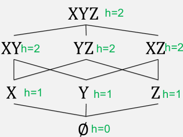
Figure 2: A relation defining the parity entropy $\bm{h}$. The marginal distribution of $X$ is $p(X=0)=p(X=1)=1/2$, hence its entropy is $h(X)=1$, and similarly for the others values.

Any entropic vector $\bm{h}\in\mathbb{R}_{+}^{2^{\bm{X}}}$ satisfies the following basic Shannon inequalities:

$$h(\emptyset)= 0$$ (13)

$$h(\bm{U}\cup\bm{V})\geq h(\bm{U})$$ (14)

$$h(\bm{U})+h(\bm{V})\geq h(\bm{U}\cup\bm{V})+h(\bm{U}\cap\bm{V})$$ (15)

The last two inequalities are called called monotonicity and submodularity respectively. A Shannon inequality is a positive linear combination of basic Shannon inequalities.

Any vector $h:2^{\bm{X}}\rightarrow\mathbb{R}_{+}$ that satisfies the basic Shannon inequalities is called a polymatroid. The set of entropic vectors is denoted by $\Gamma_{n}^{*}$ and the set of polymatroids is denoted by $\Gamma_{n}$, where $n=|\bm{X}|$ is the number of variables. The following holds: $\Gamma_{n}^{*}\subsetneq\Gamma_{n}\subsetneq{\mathbb{R}}_{\tiny+}^{2^{[n]}}$. In particular, not every polymatroid is entropic, as we will see shortly (in Fig. 5). Fig. 3 represents these two sets, as well as other sets, defined later in this paper. In some of the literature the entropic vectors and the polymatroids are defined as $(2^{n}-1)$-dimensional vectors, by dropping the $\emptyset$-dimension, because, in that case, both sets $\Gamma_{n}^{*}$ and $\Gamma_{n}$ have a non-empty interior. We prefer to use $2^{n}$ dimensions since this simplifies most of the discussion, and postpone dealing with the non-empty interior until Section 9.6.

$\Gamma_{n}$:	polymatroids
$\bar{\Gamma}_{n}^{*}$:	almost-entropic
$\Gamma_{n}^{*}$:	entropic
$\Upsilon_{n}$:	group realizable
$N_{n}$:	normal polymatroids
$M_{n}$:	modular polymatroids

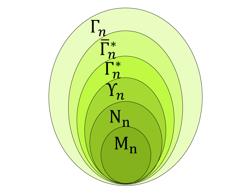
Figure 3: Landscape of polymatroids

An information inequality is an assertion stating that a linear expression of entropic terms is $\geq 0$.

Definition 4.2.

We associate to any vector $\bm{c}\in\mathbb{R}^{2^{[n]}}$ the following information inequality:

$$\sum_{\alpha\subseteq[n]}c_{\alpha}h(\bm{X}_{\alpha})\geq 0$$ (16)

By using the dot-product notation, we can write the inequality as $\bm{c}\cdot\bm{h}\geq 0$. If the inequality holds for all $h\in K$, where $K\subseteq{\mathbb{R}}_{\tiny+}^{2^{[n]}}$ is some set, then we say that it is valid for $K$, and write $K\models\bm{c}\cdot\bm{h}\geq 0$.

Thus, we will talk about inequalities valid for entropic vectors, or valid for polymatroids, and the latter are precisely the Shannon inequalities (this is implicit in the proof of Th. 5.2 below). Any Shannon inequality is also valid for entropic vectors; however, we will see in Th. 5.7 below a non-Shannon inequality, which is valid for entropic vectors, but not for polymatroids. In analogy with mathematical logic, one should think the vectors $\bm{h}$ as models, inequalities $\bm{c}\cdot\bm{h}\geq 0$ as formulas, and sets $K\subseteq{\mathbb{R}}_{\tiny+}^{2^{[n]}}$ as classes of models.

Example 4.3.

The following is a Shannon inequality, called Shearer’s inequality:

$$h(XY)+h(YZ)+h(ZX)-2h(XYZ)\geq 0$$ (17)

To prove it, we apply submodularity twice, underlining the affected terms:

$$\underline{h(XY)+h(YZ)}+h(ZX)$$

$$\ \ \ \ \geq h(XYZ)+\underline{h(Y)+h(ZX)}$$

$$\ \ \ \ \geq h(XYZ)+h(XYZ)+h(\emptyset)=2h(XYZ)$$

Equivalently, we observe that (17) is the sum of the following basic Shannon inequalities:

$$h(XY)+h(YZ)-h(Y)-h(XYZ)\geq 0$$

$$h(Y)+h(ZX)-h(\emptyset)-h(XYZ)\geq 0$$

$$h(\emptyset)= 0$$

We will prove shortly (Theorem 5.2 below) that one can decide in time exponential in $n$ whether an inequality is valid for all polymatroids. In contrast, it is an open problem whether entropic validity is decidable.

4.2 The Entropic Bound and the Polymatroid Bound

The general framework for computing a bound on a query’s output uses degree constraints, which, in turn, correspond to conditional entropies. We define these two notions first.

We write $\bm{U}\bm{V}$ for set $\bm{U}\cup\bm{V}$. Given $\bm{h}\in\mathbb{R}_{+}^{2^{[n]}}$, define:

$$h(\bm{V}|\bm{U})\stackrel{{\scriptstyle\text{def}}}{{=}} h(\bm{U}\bm{V})-h(\bm{U})$$ (18)

$\bm{U},\bm{V}$ need not be disjoint, and $h(\bm{V}|\bm{U})=h(\bm{V}-\bm{U}|\bm{U})$; for example, $h(XY|X)=h(Y|X)$. If $h(\bm{V}|\bm{U})=0$ then we say that $\bm{h}$ satisfies the functional dependency $\bm{U}\rightarrow\bm{V}$, and we write $\bm{h}\models\bm{U}\rightarrow\bm{V}$. Lee [Lee87a] proved that, if $R$ is a relation instance with attributes $\bm{X}$, $p:R\rightarrow[0,1]$ is a probability distribution, and $\bm{h}$ is its entropic vector, then $R\models\bm{U}\rightarrow\bm{V}$ iff $\bm{h}\models\bm{U}\rightarrow\bm{V}$. For a simple illustration, referring to Fig. 2, both $R$ and its entropy $\bm{h}$ satisfy the FDs $XY\rightarrow Z$, $XZ\rightarrow Y$, and $YZ\rightarrow X$: for example $XY$ is a key (all 4 tuples have distinct values $XY$) and $h(Z|XY)=h(XYZ)-h(XY)=2-2=0$.

Fix $\bm{U}$, and denote by $h(-|\bm{U}):2^{\bm{X}-\bm{U}}\rightarrow\mathbb{R}_{+}$ the function $\bm{V}\mapsto h(\bm{V}|\bm{U})$. If $\bm{h}$ is a polymatroid, then $h(-|\bm{U})$ is also a polymatroid, called the conditional polymatroid. If $\bm{h}$ is an entropic vector, then, surprisingly, $\bm{h}(-|\bm{U})$ is not necessarily entropic (as we will see later in Sec. 9.3), yet the name conditional entropy is justified by the following. Suppose $\bm{h}$ is associated to $(R,p)$. Fix an outcome $\bm{u}\in\textsf{Dom}^{\bm{U}}$, consider the random variable $\bm{V}$ conditioned on $\bm{U}=\bm{u}$, and denote its entropy by $h(\bm{V}|\bm{U}=\bm{u})$. Then:

$$h(\bm{V}|\bm{U})= \mathop{\mathbb{E}}_{\bm{u}}\left[h(\bm{V}|\bm{U}=\bm{u})\right]$$ (19)

In other words, $h(\bm{V}|\bm{U})$ equals the expectation over the outcomes $\bm{u}$ of the (standard) entropy of the random variable $\bm{V}$ conditioned on $\bm{U}=\bm{u}$. The proof of identity (19) consists of applying directly the definition of the entropy given in Eq. (12).

When proving Shannon inequalities it is sometimes convenient to write the submodularity inequality as $h(\bm{V}|\bm{U})\geq h(\bm{V}|\bm{U}\bm{W})$. In other words, conditioning on more variables can only decrease the entropy.

Example 4.4.

We illustrate a simple Shannon inequality with conditionals:

$$\underline{h(XY)} \underline{+h(YZ)}+h(ZU)+h(U|XZ)+h(X|YU)\geq$$

$$\geq h(XYZ)+\underline{h(Y)+h(ZU)}+h(U|XZ)+h(X|YU)$$

$$\geq h(XYZ)+h(YZU)+\underline{h(U|XZ)}+\underline{h(X|YU)}$$

$$\geq h(XYZ)+h(YZU)+h(U|XYZ)+h(X|YZU)$$

$$= 2h(XYZU)$$

Next, we define degrees of a relation instance $R\subseteq\textsf{Dom}^{\bm{X}}$. Given subsets $\bm{U},\bm{V}\subseteq\bm{X}$, and $\bm{u}\in\textsf{Dom}^{\bm{U}}$, the $\bm{V}$-degree of $\bm{U}=\bm{u}$ in $R$ is the number of distinct values $\bm{v}$ that occur in $R$ together with $\bm{u}$; the max-$\bm{V}$-degree of $\bm{U}$ is the maximum degree over all values $\bm{u}$. Formally:

$$\texttt{deg}_{R}(\bm{V}|\bm{U}=\bm{u})\stackrel{{\scriptstyle\text{def}}}{{=}} \left|\{{\bm{v}}\mid{(\bm{u},\bm{v})\in\Pi_{\bm{U}\bm{V}}(R)}\}\right|$$

$$\texttt{deg}_{R}(\bm{V}|\bm{U})\stackrel{{\scriptstyle\text{def}}}{{=}} \max_{\bm{u}}\left(\texttt{deg}_{R}(\bm{V}|\bm{U}=\bm{u})\right)$$

We note that $\texttt{deg}_{R}(\bm{V}|\bm{U})\geq 1$ (since we assumed $R\neq\emptyset$), and equality holds iff $R$ satisfies the functional dependency $\bm{U}\rightarrow\bm{V}$.

Definition 4.5.

Fix a relation $R(\bm{X})$. A degree statistics, or a statistics in short, $\sigma$, is an expression of the form $\sigma=(\bm{V}|\bm{U})$ where $\bm{U},\bm{V}\subseteq\bm{X}$; when $\bm{U}=\emptyset$ then we call $\sigma$ a cardinality statistics, and write it as $(\bm{V})$. If $\Sigma$ is a set of statistics, then we call $\bm{B}=(B_{\sigma})_{\sigma\in\Sigma}$, where $B_{\sigma}\geq 1$, statistics values associated to $\Sigma$. The log-statistics values are $\bm{b}=\log\bm{B}=(b_{\sigma}:=\log B_{\sigma})_{\sigma\in\Sigma}$.

We abbreviate $h(\bm{V}|\bm{U})$ and $\texttt{deg}_{R}(\bm{V}|\bm{U})$ with $h(\sigma)$ and $\texttt{deg}_{R}(\sigma)$ respectively. If $\Sigma$ is a set of statistics, then a $\Sigma$-inequality is an inequality of the following form:

$$\sum_{\sigma\in\Sigma}w_{\sigma}h(\sigma)\geq h(\bm{X})$$ (20)

where $\bm{w}=(w_{\sigma})_{\sigma\in\Sigma}$ are nonnegative weights.

Fix a hypergraph $\mathcal{H}=(\bm{X},E)$. We say that $\Sigma$ is guarded by $\mathcal{H}$ if, for every $\sigma=(\bm{V}|\bm{U})$ in $\Sigma$, there exists a hyperedge $\bm{Y}_{\sigma}\in E$ such that $\bm{U},\bm{V}\subseteq\bm{Y}_{\sigma}$; we call $\bm{Y}_{\sigma}$ the guard of $\sigma$. When $\mathcal{H}$ is the hypergraph of a query $Q$, then we say that $\Sigma$ is guarded by $Q$, and that $R_{\sigma}$ is the guard of $\sigma$. The following theorem establishes the key connection between information inequalities and query output size. The proof relies on a method originally introduced by Chung et al. for a combinatorial problem [CGFS86], and adapted by Grohe and Marx for constraint satisfaction [GM14], then by Atserias, Grohe, and Marx for their AGM bound [AGM13].

Theorem 4.6.

Assume $\Sigma$ is guarded by $Q$. If the $\Sigma$-inequality (20) is valid for entropic vectors then:

$$|Q|\leq \prod_{\sigma\in\Sigma}\texttt{deg}_{R_{\sigma}}^{w_{\sigma}}(\sigma)$$ (21)

where $R_{\sigma}$ is the guard of $\sigma\in\Sigma$.

Proof.

Fix a database instance $\bm{D}$, and let $\bm{h}$ be the entropic vector associated to the relation $Q(\bm{D})$; by uniformity, $h(\bm{X})=\log|Q(\bm{D})|$. If $\sigma=(\bm{V}|\bm{U})\in\Sigma$ has guard $R_{\sigma}$, then:

$$h(\sigma)= \mathop{\mathbb{E}}_{\bm{u}}\left[h(\bm{V}|\bm{U}=\bm{u})\right]\leq\max_{\bm{u}}h(\bm{V}|\bm{U}=\bm{u})$$

$$\leq \max_{\bm{u}}\log\deg_{R_{\sigma}}(\bm{V}|\bm{U}=\bm{u})$$

$$= \log\deg_{R_{\sigma}}(\bm{V}|\bm{U})=\log\deg_{R_{\sigma}}(\sigma)$$

Using (20) we derive:

$$\sum_{\sigma}w_{\sigma}\log\deg_{R_{\sigma}}(\sigma)\geq \sum_{\sigma}w_{\sigma}h(\sigma)\geq h(\bm{X})=\log|Q|$$

∎

Inequality (20) is similar to the AGM inequality (6). Next, we proceed as we did for the AGM bound: fix numerical values for the statistics, then minimize the bound over all valid $\bm{w}$’s. We say that a database instance $\bm{D}$ satisfies the statistics $\Sigma,\bm{B}$, in notation $\bm{D}\models(\Sigma,\bm{B})$, if $\texttt{deg}_{R_{\sigma}^{\bm{D}}}(\sigma)\leq B_{\sigma}$ for all $\sigma\in\Sigma$. Similarly, we say that a vector $\bm{h}$ satisfies the log-statistics $\Sigma,\bm{b}$ if $h(\sigma)\leq b_{\sigma}$ for all $\sigma$. We define:

Definition 4.7 (Query Upper Bound).

Let $\Sigma,\bm{B}$ be statistics values, guarded by the query $Q$. Fix some set $K\subseteq\mathbb{R}^{2^{[n]}}$. The Upper Bound w.r.t. $K$ of the query $Q$ is:

$$\text{U-Bound}_{K}(Q,\Sigma,\bm{B})\stackrel{{\scriptstyle\text{def}}}{{=}} \inf_{\bm{w}:K\models\mbox{Eq.\eqref{eq:conditional:ii}}}\prod_{\sigma\in\Sigma}B_{\sigma}^{w_{\sigma}}$$

The entropic upper bound is $\text{U-Bound}_{\Gamma_{n}^{*}}$ and the polymatroid upper bound is $\text{U-Bound}_{\Gamma_{n}}$.

Sometimes it is more convenient to use the logarithm and define:

$$\text{Log-U-Bound}_{K}(Q,\Sigma,\bm{b})\stackrel{{\scriptstyle\text{def}}}{{=}} \inf_{\bm{w}:K\models\mbox{Eq.\eqref{eq:conditional:ii}}}\sum_{\sigma\in\Sigma}w_{\sigma}b_{\sigma}$$ (22)

Corollary 4.8.

The following hold:

• $\text{U-Bound}_{\Gamma_{n}^{*}}(Q,\Sigma,\bm{B})\leq\text{U-Bound}_{\Gamma_{n}}(Q,\Sigma,\bm{B})$, and

• If $\bm{D}\models(\Sigma,\bm{B})$ then $|Q(\bm{D})|\leq\text{U-Bound}_{\Gamma_{n}^{*}}(Q,\Sigma,\bm{B})$.

The first item is by $\Gamma_{n}^{*}\subseteq\Gamma_{n}$, the second is by Th. 4.6.

Let’s compare these bound with the AGM bound (7). There, we had to minimize an expression where $\bm{w}$ ranged over the fractional edge covers of the query’s hypergraph. In our new setting, $\bm{w}$ ranges over valid $\Sigma$-inequalities, a much more difficult task. To compute the polymatroid bound, $\bm{w}$ ranges over $\Sigma$-inequalities valid for polymatroids, and we will show in Th. 5.2 that this bound can be computed in time exponential in $n$. However, in order to compute the entropic bound, $\bm{w}$ needs to define a valid entropic inequality, and it is currently open whether this bound is computable. On the other hand, we will prove that the entropic bound is asymptotically tight, while the polymatroid bound is not. Thus, we are faced with a difficult choice, between and exact but non-computable bound, or a computable but inexact bound. This justifies examining non-trivial special cases of statistics $\Sigma$ when these two bounds agree. We illustrate the entropic upper bound with an example.

Example 4.9.

Consider the following conjunctive query:

$$Q(X,Y,Z,U)= R(X,Y)\wedge S(Y,Z)\wedge T(Z,U)$$

$$\wedge A(X,Z,U)\wedge B(X,Y,U)$$

Suppose that we are given the following set of statistics $\Sigma=\{(XY),(YZ),(ZU),(U|XZ),(X|YU)\}$. In other words, we have bounds on the cardinalities of $R,S,T$, but not of $A,B$, hence we can assume that $|A|=|B|=\infty$. Instead, we have the statistics $\texttt{deg}_{A}(U|XZ)$ and $\texttt{deg}_{B}(X|YU)$. The AGM bound (6) is $|Q|\leq|R|\cdot|T|$, because the only fractional edge cover whose bound is $<\infty$ is $w_{R}=w_{T}=1$ and $w_{S}=w_{A}=w_{B}=0$.

The polymatroid bound follows from these $\Sigma$-inequalities:

$$h(XY)+h(YZ)+h(ZU)+h(U|XZ)+h(X|YU)\geq$$

$$\hskip 142.26378pt\geq 2h(XYZU)$$

$$h(XY)+h(ZU)\geq h(XYZU)$$

$$h(XY)+h(YZ)+h(U|XZ)\geq h(XYZU)$$

$$h(YZ)+h(ZU)+h(X|YU)\geq h(XYZU)$$

We proved the first inequality in Example 4.4, while the other three are immediate. They imply:

$$|Q|\leq \big{(}|R|\cdot|S|\cdot|T|\cdot\texttt{deg}_{A}(U|XZ)\cdot\texttt{deg}_{B}(X|YU)\big{)}^{1/2}$$

$$|Q|\leq |R|\cdot|T|$$

$$|Q|\leq |R|\cdot|S|\cdot\texttt{deg}_{B}(X|YU)$$

$$|Q|\leq |S|\cdot|T|\cdot\texttt{deg}_{A}(U|XZ)$$

The AGM bound is the second inequality. We show in Appendix .1 that the entropic bound is the minimum over all four expressions above. (This requires proving that there is no “better” inequality that gives us a smaller bound.) Since all four inequalities are Shannon inequalities, it follows that, in this case, the entropic bound is equal to the polymatroid bound.

When $XZ$ is a key in $A$, and $YU$ is a key in $B$, then the polymatroid bound simplifies to:

$$|Q|\leq\min((|R|\cdot|S|\cdot|T|)^{1/2},|R|\cdot|T|,|R|\cdot|S|,|S|\cdot|T|)$$

Special Case: Cardinality Constraints We show next that the AGM bound is a special case where the polymatroid and entropic bounds coincide; we will see a more general setting when this happens in Sec. 6. Assume $\Sigma$ is restricted to cardinality constraints, and assume for simplicity that $\Sigma$ has exactly one cardinality constraint $(\bm{Y}_{j})$ for each relation $R_{j}(\bm{Y}_{j})$ in the query; $\Sigma=\{(\bm{Y}_{1}),\ldots,(\bm{Y}_{m})\}$. The $\Sigma$-inequality (20) becomes:

$$\sum_{j=1,m}w_{j}h(\bm{Y}_{j})\geq h(\bm{X})$$ (23)

When $w_{1}=\cdots=w_{m}$ then (23) is called Shearer’s inequality.

Theorem 4.10.

The following are equivalent:

1. Inequality (23) is valid for polymatroids.

2. Inequality (23) is valid for entropic functions.

3. The weights $\bm{w}$ form a fractional edge cover of the hypergraph $(\bm{X},\{{\bm{Y}_{j}}\mid{j=1,m}\})$.

$$R= \begin{array}[]{|ccc|c}\cline{1-3}\cr X_{1}\ldots X_{i-1}&X_{i}&X_{i+1}\ldots X_{n}&p\\ \cline{1-3}\cr 0\ \ \ \ldots\ \ \ 0&0&0\ \ \ \ldots\ \ \ 0&1/2\\ 0\ \ \ \ldots\ \ \ 0&1&0\ \ \ \ldots\ \ \ 0&1/2\\ \cline{1-3}\cr\end{array} h^{X_{i}}(\bm{U})=\begin{cases}1&\mbox{if $X_{i}\in\bm{U}$}\\ 0&\mbox{if $X_{i}\not\in\bm{U}$}\end{cases}$$

Figure 4: A relation $R$ with two tuples that agree on all attributes, except $X_{i}$. Its entropic vector is called the basic modular function, $\bm{h}^{X_{i}}$; it is used in Th. 4.10, and discussed in more detail in Sec. 6.

Proof.

i $\Rightarrow$ ii is immediate. For ii $\Rightarrow$ iii, assume that (23) holds for all entropic vectors, and consider any variable $X_{i}\in\bm{X}$, for $i=1,n$. Consider the basic modular entropic function $\bm{h}^{X_{i}}$ shown in Fig. 4. Since $\bm{h}^{X_{i}}$ satisfies inequality (23), it follows that $\sum_{j=1,m:X_{i}\in\bm{Y}_{j}}w_{j}\geq 1$ (because $h^{X_{i}}(\bm{Y}_{j})=1$ iff $X_{i}\in\bm{Y}_{j}$), proving that $\bm{w}$ is a fractional edge cover.

It remains to prove the implication iii $\Rightarrow$ i. This is a well known result, and it admits multiple proofs (we give a second proof in Sec. 7.2). Here, we will prove the inequality by induction on $n$:

• Partition the set of indices $j$ into $J_{0}$ and $J_{1}$:
  $J_{0}\stackrel{{\scriptstyle\text{def}}}{{=}}\{{j}\mid{X_{n}\not\in\bm{Y}_{j}}\}$, $J_{1}\stackrel{{\scriptstyle\text{def}}}{{=}}\{{j}\mid{X_{n}\in\bm{Y}_{j}}\}$.

• If $j\in J_{1}$ then write $h(\bm{Y}_{j})=h(X_{n})+h(\bm{Y}_{j}-X_{n}|X_{n})$. Note that $\sum_{j\in J_{1}}w_{j}\geq 1$ because $X_{n}$ is covered.

• If $j\in J_{0}$ then write $h(\bm{Y}_{j})\geq h(\bm{Y}_{j}-X_{n}|X_{n})$.

Using the steps above we obtain:

$$\sum_{j}w_{j}h(\bm{Y}_{j})\geq h(X_{n})+\sum_{j}w_{j}h(\bm{Y}_{j}-X_{n}|X_{n})$$

$$\geq h(X_{n})+h(\bm{X}-X_{n}|X_{n})=h(\bm{X})$$

The last line used induction on the polymatroid $h(-|X_{n})$. ∎

It follows immediately that the AGM bound, the entropic bound, and the polymatroid bound coincide in the simple case when the statistics are restricted to the cardinalities of the input relations.

Discussion Degree constraints occur often and naturally in database applications. For example, if a relation $R_{j}(\bm{Y}_{j})$ has a key $\bm{U}$, then $\texttt{deg}_{R_{j}}(\bm{Y}_{j}|\bm{U})=1$. In practice almost every relation has a key, so this case is very common. In other cases some cardinality constraints can be obtained directly from the application. For example, suppose that in a database of customers we require that no customer may have more than 10 credit cards, which naturally leads to a max-degree constraint. Such constraints are used in some modern systems, for example in scale-independent query processing [AFP⁺09, ACK⁺11, ALK⁺13].

5 The Worst-Case Instance

Informally, we call a database instance $\bm{D}$ a worst-case instance if it satisfies the given statistics, and the query’s output is as large as, or approaches asymptotically (in a sense to be made precise), the entropic upper bound. We will show that such a worst-case instance exists, proving that the entropic bound is asymptotically tight, which is a weaker notion of tightness than for the AGM bound in Th. 3.4. We will also show that, in general, the polymatroid bound is not tight, even for this weaker notion of tightness.

To construct the worst-case instance we need a dual definition of the entropic and polymatroid bounds. We define them directly using log-version:

Definition 5.1 (Query Lower Bound).

Fix log-statistics $\Sigma,\bm{b}$. For any set $K\subseteq\mathbb{R}^{2^{[n]}}$, the Log Lower Bound w.r.t. $K$ is:

$$\text{Log-L-Bound}_{K}(Q,\Sigma,\bm{b})\stackrel{{\scriptstyle\text{def}}}{{=}} \sup_{\bm{h}\in K:\bm{h}\models(\Sigma,\bm{b})}h(\bm{X})$$ (24)

As before, the entropic log-lower bound is $\text{Log-L-Bound}_{\Gamma_{n}^{*}}$, and the polymatroid log-lower bound is $\text{Log-L-Bound}_{\Gamma_{n}}$.

The log-lower bound asks us to find a vector $\bm{h}$ that satisfies all log-statistics $\Sigma,\bm{b}$, and where $\bm{h}(\bm{X})$ is as large as possible. We call $\bm{h}$ a worst case entropic vector, or the worst case polymatroid respectively. Using $\bm{h}$, we would like to construct a worst-case database instance $\bm{D}$, that satisfies $\Sigma,\bm{B}$, and $\log|Q(\bm{D})|=h(\bm{X})$. The difficulty lies in the fact that, when $\bm{h}$ is a polymatroid then such a database may not exists general, and when $\bm{h}$ is an entropic vector, then it may be realized by a probability space that is non-uniform, hence we cannot use it to construct $\bm{D}$. We start by observing the following, which is easy to check:

$$\text{Log-L-Bound}_{K}(Q,\Sigma,\bm{b})\leq \text{Log-U-Bound}_{K}(Q,\Sigma,\bm{b})$$ (25)

Indeed, if $\bm{h}\in K$ satisfies $\bm{h}\models(\Sigma,\bm{b})$, and $\bm{w}$ satisfies $\forall\bm{h}\in K,\sum_{\sigma}w_{\sigma}h(\sigma)\geq h(\bm{X})$, then $h(\bm{X})\leq\sum_{\sigma}w_{\sigma}h(\sigma)\leq\sum_{\sigma}w_{\sigma}b_{\sigma}$, and the claim follows from $\text{Log-L-Bound}_{K}=\sup_{\bm{h}}h(\bm{X})\leq\text{Log-U-Bound}_{K}=\inf_{\bm{w}}\sum_{\sigma}w_{\sigma}b_{\sigma}$.

When $K=\Gamma_{n}$, then [KNS17] showed that the two bounds are equal. We prove a slightly more general statement:

Theorem 5.2.

Suppose the set $K$ is defined by linear constraints: $K=\{{\bm{h}\in{\mathbb{R}}_{\tiny+}^{2^{[n]}}}\mid{\bm{M}\cdot\bm{h}\geq 0}\}$, where $\bm{M}$ is some matrix. Then, $\text{Log-L-Bound}_{K}$ and $\text{Log-U-Bound}_{K}$ are defined by a pair of primal/dual linear programs, with a number of variables exponential in $n$; the expressions $\inf,\sup$ in (22),  (24) can be replaced by $\min,\max$; and Eq. (25) becomes an equality, $h^{*}(\bm{X})=\sum_{\sigma}w^{*}_{\sigma}b_{\sigma}$, where $\bm{h}^{*}$, $\bm{w}^{*}$ are the optimal solutions of the primal and dual program respectively.

Proof.

Denote $s=|\Sigma|$, and let $\bm{A}$ be the $s\times 2^{n}$ matrix that maps $\bm{h}$ to the vector $\bm{A}\cdot\bm{h}=(h(\sigma))_{\sigma\in\Sigma}\in\mathbb{R}^{s}$. Let $\bm{c}\in\mathbb{R}^{2^{n}}$ be the vector $c_{\bm{X}}=1$, $c_{\bm{U}}=0$ for $\bm{U}\neq\bm{X}$. The two bounds are the optimal solutions to the following pair of primal/dual linear programs:

$$\begin{array}[]{ll|ll}\lx@intercol\text{Log-L-Bound}_{K}\hfil\lx@intercol\vrule\lx@intercol&\vrule\lx@intercol\text{Log-U-Bound}_{K}\hfil\lx@intercol\\ \hline\cr\lx@intercol\mbox{Maximize }\bm{c}^{T}\cdot\bm{h}\hfil\lx@intercol\vrule\lx@intercol&\vrule\lx@intercol\mbox{Minimize }\bm{w}^{T}\cdot\bm{b}\hfil\lx@intercol\\ \mbox{where}&\bm{A}\cdot\bm{h}\leq\bm{b}&\mbox{where}&\bm{w}^{T}\cdot\bm{A}-\bm{c}^{T}\geq\bm{u}^{T}\cdot\bm{M}\\ &-\bm{M}\cdot\bm{h}\leq 0&&\end{array}$$

where the primal variables are $\bm{h}\geq 0$, and the dual variables are $\bm{w},\bm{u}\geq 0$; the reader may check that the two programs above form indeed a primal/dual pair. $\text{Log-L-Bound}_{K}$ is by definition the optimal value of the program above. We prove that $\text{Log-U-Bound}_{K}$ is the value of the dual. First, observe that the $\Sigma$-inequality (20) is equivalent to $(\bm{w}^{T}\cdot\bm{A}-\bm{c}^{T})\cdot h\geq 0$. We claim that this inequality holds $\forall\bm{h}\in K$ iff there exists $\bm{u}$ s.t. $(\bm{w},\bm{u})$ is a feasible solution to the dual. For that consider the following primal/dual programs with variables $\bm{h}\geq 0$ and $\bm{u}\geq 0$ respectively:

$$\begin{array}[]{ll|ll}\lx@intercol\mbox{Minimize }(\bm{w}^{T}\cdot\bm{A}-\bm{c}^{T})\cdot\bm{h}\hfil\lx@intercol\vrule\lx@intercol&\vrule\lx@intercol\mbox{Maximize }0\hfil\lx@intercol\\ \mbox{where}&\bm{M}\cdot\bm{h}\geq 0&\mbox{where}&\bm{u}^{T}\cdot\bm{M}\leq\bm{w}^{T}\bm{A}-\bm{c}^{T}\end{array}$$

The primal (left) has optimal value 0 iff the inequality $(\bm{w}^{T}\cdot\bm{A}-\bm{c}^{T})\cdot\bm{h}\geq 0$ holds forall $\bm{h}\in K$; otherwise its optimal is $-\infty$. The dual (right) has optimal value 0 iff there exists a feasible solution $\bm{u}$; otherwise its optimal is $-\infty$. Strong duality proves our claim. ∎

When $K=\Gamma_{n}^{*}$, then the two terms in (25) may no longer be equal in general, but we prove that they are equal asymptotically. Call a $k$-amplification of a set of log-statistics $\Sigma,\bm{b}$ the log-statistics $\Sigma,k\bm{b}$, where $k$ is a natural number. Observe that the entropic log-upper bound increases linearly with the $k$-amplification:

$$\text{Log-U-Bound}_{\Gamma_{n}^{*}}(Q,\Sigma,k\bm{b})= k\text{Log-U-Bound}_{\Gamma_{n}^{*}}(Q,\Sigma,\bm{b})$$ (26)

The lower bound increases at least linearly, $\text{Log-L-Bound}_{\Gamma_{n}^{*}}(Q,\Sigma,k\bm{b})\geq k\text{Log-L-Bound}_{\Gamma_{n}^{*}}(Q,\Sigma,\bm{b})$, because of the following proposition:

Proposition 5.3.

If $\bm{h}_{1},\bm{h}_{2}$ are two entropic vectors, then so is $\bm{h}_{1}+\bm{h}_{2}$.

Proof.

Suppose $\bm{h}_{1},\bm{h}_{2}$ are realized by two finite probability spaces $(R_{1},p_{1}),(R_{2},p_{2})$. Then their sum is realized by $(R_{1}\otimes R_{2},p)$ (see Def. 2.1), where $p(\bm{x}_{1}\otimes\bm{x}_{2})\stackrel{{\scriptstyle\text{def}}}{{=}}p(\bm{x}_{1})\cdot p(\bm{x}_{2})$. ∎

We prove:

Theorem 5.4.

Fix any $Q,\Sigma,\bm{b}$. The entropic upper and lower bounds are asymptotically equal, in the following sense:

$$\sup_{k}\frac{\text{Log-L-Bound}_{\Gamma_{n}^{*}}(Q,\Sigma,k\bm{b})}{\text{Log-U-Bound}_{\Gamma_{n}^{*}}(Q,\Sigma,k\bm{b})}= 1$$ (27)

The proof of this result, which appears to be novel, requires a discussion of the set of almost-entropic functions, and we defer this to Sec. 9.

Finally, we can answer the central question in this section: the entropic bound is tight asymptotically, while the polymatroid bound is not.

Theorem 5.5.

(1) For any query $Q$ and statistics $\Sigma,\bm{B}$, the entropic bound is asymptotically tight, in the following sense:

$$\sup_{k}\frac{\sup_{\bm{D}:\bm{D}\models\bm{B}^{k}}\log|Q(\bm{D})|}{\text{Log-L-Bound}_{\Gamma_{n}^{*}}(Q,\Sigma,k\bm{b})}= 1$$ (28)

(2) The polymatroid bound is not asymptotically tight: there exists a query $Q$ and statistics $\Sigma,\bm{B}$ such that:

$$\sup_{k}\frac{\sup_{\bm{D}:\bm{D}\models\bm{B}^{k}}\log|Q(\bm{D})|}{\text{Log-L-Bound}_{\Gamma_{n}}(Q,\Sigma,k\bm{b})}\leq \frac{43}{44}$$ (29)

Here $\bm{B}^{k}\stackrel{{\scriptstyle\text{def}}}{{=}}(B^{k}_{\sigma})_{\sigma\in\Sigma}$, and $\bm{b}\stackrel{{\scriptstyle\text{def}}}{{=}}\log\bm{B}$. Moreover, this property holds even if $\Sigma,\bm{B}$ consists only of cardinality constraints and functional dependencies, i.e. $\forall\sigma\in\Sigma$ either $\sigma=(\bm{V})$ or $B_{\sigma}=1$.

Equivalently, Eq. (28) says that, for any statistics $\Sigma,\bm{B}$, if we allow a sufficiently large amplification $\Sigma,\bm{B}^{k}$, then there exists a worst-case instance $\bm{D}$ satisfying the amplified statistics such that $\log|Q(\bm{D})|$ approaches $\text{L-Bound}_{\Gamma_{n}^{*}}(Q,\Sigma,\bm{B}^{k})$. Notice that this is a weaker notion of tightness than for the AGM bound in Theorem 3.4. There, tightness referred to the ratio betwen the lower and upper bound, while here tightness refers to the ratio of their logarithms, a weaker notion. Eq. (29) says that even this weaker tightness fails for the polymatroid bound.

The first proof of asymptotic tightness was given by Gogacz and Torunczyk [GT17], for the restricted case when the statistics are either cardinalities, or functional dependencies. The general case was proven in [KNS17]. Both results were stated slightly differently from ours, by using almost-entropic functions. We prefer to state our result in terms of the entropic functions, since it is more natural, and defer the discussion of almost entropic functions to Sec. 9, where they have a very natural justification.

In the rest of this section we prove Theorem 5.5. We use this opportunity to continue our dive into the fascinating world of entropic functions, and non-Shannon inequalities, which are needed for the proof. However, the rest of this section is rather technical, and readers not interested in this background may safely skip the rest of this section, since we do not need it, except for the short introduction of mutual information.

5.1 Background: Non-Shannon Inequalities, Lattices, Groups

Mutual Information Given a vector $\bm{h}\in\mathbb{R}^{2^{[n]}}$ and three disjoint sets of variables $\bm{U},\bm{V},\bm{W}\subseteq\bm{X}$, we denote by:

$$I_{h}(\bm{V};\bm{W}|\bm{U})\stackrel{{\scriptstyle\text{def}}}{{=}} h(\bm{U}\bm{V})+h(\bm{U}\bm{W})-h(\bm{U})-h(\bm{U}\bm{V}\bm{V})$$ (30)

When $h$ is clear from the context, then we will drop the index $h$ from $I_{h}$ and write simply $I$. When $h$ is an entropic vector, then $I_{h}(\bm{V};\bm{W}|\bm{U})$ is called the mutual information of $\bm{V},\bm{W}$ conditioned on $\bm{U}$. In that case, $I_{h}(\bm{V};\bm{W}|\bm{U})=0$ iff the probability space realizing $h$ satisfies $\bm{V}\perp\bm{W}|\bm{U}$, meaning that $\bm{V},\bm{W}$ are independent conditioned on $\bm{U}$. With some abuse, we will call $I_{h}$ a conditional mutual information even when $\bm{h}$ is a polymatroid. The following properties hold:

Proposition 5.6.

For any polymatroid $h$:

• $I_{h}(\bm{V};\bm{W}|\bm{U})\geq 0$ (this is a submodularity inequality).

• The chain rule holds:
  $I_{h}(\bm{U}\bm{V};\bm{W}|\bm{Z})=I_{h}(\bm{U};\bm{W}|\bm{Z})+I_{h}(\bm{V};\bm{W}|\bm{U}\bm{Z})$.

• An elemental mutual information term is an expression of the form $I_{h}(X_{i};X_{j}|\bm{U})$, where $X_{i}\neq X_{j}\not\in\bm{U}$ are single variables. Every mutual information $I(\bm{V};\bm{W}|\bm{U})$ is the sum of elemental terms.

• For any subsets $\bm{U}_{0}\subseteq\bm{U}$ and $\bm{V}_{0}\subseteq\bm{V}$:

  $$I_{h}(\bm{U}_{0};\bm{V}_{0}|\bm{Z})\leq I_{h}(\bm{U};\bm{V}|\bm{Z})$$ (31)

  If $I_{h}(\bm{U};\bm{V}|\bm{Z})=0$, then $I_{h}(\bm{U}_{0};\bm{V}_{0}|\bm{Z})=0$.

Non-Shannon inequalities The first non-Shannon inequality was proven by Zhang and Yeung [ZY98]. We review it here, following the simplified presentation by Romashchenko [Rom22] (see also Csirmaz [Csi22]).

Zhang and Yeung [ZY98] proved the following:

Theorem 5.7.

The following is a non-Shannon inequality:

$$I_{h}(X;Y)\leq I_{h}(X;Y|A)+I_{h}(X;Y|B)+I_{h}(A;B)$$ (32)

$$+ I_{h}(X;Y|A)+I_{h}(A;Y|X)+I_{h}(A;X|Y)$$

In other words, this inequality is valid for entropic vectors, but it cannot be proven using the basic Shannon inequalities, hence the term non-Shannon. The proof of this inequality, and that of several other non-Shannon inequalities proven after 1998, relies on the following copy lemma.

Lemma 5.8 (Copy Lemma).

Let $\bm{X},\bm{Y}$ be two disjoint sets of variables, and let $\bm{h}$ be an entropic vector with variables $\bm{X}\bm{Y}$. Let $\bm{Y}^{\prime}$ be fresh copies of the variables $\bm{Y}$. Thus, each variable $Y\in\bm{Y}$ has a copy $Y^{\prime}\in\bm{Y}^{\prime}$. Then there exists an entropic vector $\bm{h}^{\prime}$ over variables $\bm{X}\bm{Y}\bm{Y}^{\prime}$ such that the following hold:

$$I_{h^{\prime}}(\bm{Y};\bm{Y}^{\prime}|\bm{X})=0$$

$$\forall\bm{U}\subseteq\bm{X}\bm{Y}:\ \ h^{\prime}(\bm{U})=h(\bm{U})$$

$$\forall\bm{U}^{\prime}\subseteq\bm{X}\bm{Y}^{\prime}:\ \ h^{\prime}(\bm{U}^{\prime})=h(\bm{U})$$

We say that $\bm{Y}^{\prime}$ is a copy of $\bm{Y}$ over $\bm{X}$.

The first inequality asserts $\bm{Y}\perp\bm{Y}^{\prime}|\bm{X}$. The second asserts that $\bm{h},\bm{h}^{\prime}$ agree on $\bm{X}\bm{Y}$. And the last equality asserts that $\bm{h}^{\prime}$ on $\bm{X}\bm{Y}^{\prime}$ is identical to $\bm{h}$ on $\bm{X}\bm{Y}$ up to the renaming of variables from $\bm{Y}^{\prime}$ to $\bm{Y}$ (assuming $X^{\prime}=X$ for $X\in\bm{U}$).

Proof.

(of Lemma 5.8) Let $p$ be a probability distribution of random variables $\bm{X}\bm{Y}$ that realizes the entropic vector $\bm{h}$. Define the following probability distribution $p^{\prime}$ of random variables $\bm{X}\bm{Y}\bm{Y}^{\prime}$: the domains of the variables $\bm{Y}^{\prime}$ is the same as that of $\bm{Y}$, and for all outcomes $(\bm{x},\bm{y},\bm{y}^{\prime})$, $p^{\prime}(\bm{X}=\bm{x},\bm{Y}=\bm{y},\bm{Y}^{\prime}=\bm{y}^{\prime})\stackrel{{\scriptstyle\text{def}}}{{=}}$ $\frac{p(\bm{X}=\bm{x},\bm{Y}=\bm{y})p(\bm{X}=\bm{x},\bm{Y}=\bm{y}^{\prime})}{p(\bm{X}=\bm{x})}$. The claims in the lemma are easily verified. ∎

In general, the copy lemma does not hold for polymatroids, as we will see shortly. We prove now Zhang and Yeung’s inequality (32). Start from the following Shannon inequality over 5 variables, $X,Y,A,B,A^{\prime}$:

$$I_{h} (X;Y)\leq I_{h}(X;Y|A)+I_{h}(X;Y|B)+I_{h}(A;B)+$$

$$+ I_{h}(X;Y|A^{\prime})+I_{h}(A^{\prime};Y|X)+I_{h}(A^{\prime};X|Y)+$$

$$+ 3I_{h}(A^{\prime};AB|XY)$$ (33)

While this is “only” a Shannon inequality, it is surprisingly difficult to prove; we invite the readers to try it themselves, but, for completeness, we give the proof in Appendix .2. Consider now an entropic vector $\bm{h}$ over four variables, $X,Y,A,B$. We apply the copy lemma, and copy $AB$ over $XY$, resulting in an entropic vector $h^{\prime}$ with variables $X,Y,A,B,A^{\prime},B^{\prime}$. In particular, $h^{\prime}$ satisfies (33) (we don’t use $B^{\prime}$). Now we observe that (a) $I(A^{\prime};AB|XY)=0$, and (b) every occurrence of $A^{\prime}$ in the second line can be replaced by $A$; for example $I(X;Y|A^{\prime})=I(X;Y|A)$, because $I(X;Y|A^{\prime})$ is expressed in terms of $h(A^{\prime}),h(XA^{\prime}),h(YA^{\prime}),h(XYA^{\prime})$, which are equal to their copies $h(A),h(XA),h(YA),h(XYA)$. Thus, inequality (33) becomes (32), proving that (32) is valid for all entropic functions $\bm{h}$.

It remains to prove that (32) is not a Shannon inequality, and for that it suffices to describe one polymatroid that fails the inequality. To “see” this polymatroid, it is best to view it as being defined over a lattice. We take this opportunity to discuss another important concept: polymatroids on lattices.

Polymatroids on lattices A polymatroid on a lattice $(L,\preceq)$ is a function $h:L\rightarrow\mathbb{R}_{+}$ satisfying:

$$h(\hat{0})= 0$$

$$h(x\vee y)\geq h(x)$$ monotonicity

$$h(x)+h(y)\geq h(x\vee y)+h(x\wedge y)$$ submodularity

Let $\bm{X}$ be a set of $n$ variables, and $\Sigma$ a set of functional dependencies for $\bm{X}$. Recall from Sec. 2 that $(L_{\Sigma},\subseteq)$ is the lattice of closed sets. If a (standard) polymatroid $h\in\Gamma_{n}$ satisfies the functional dependencies $\Sigma$, then it is not hard to see that its restriction to $L_{\Sigma}$ is a polymatroid on $L_{\Sigma}$. Conversely, any polymatroid $\bm{h}$ on the lattice $(L_{\Sigma},\subseteq)$ can be extended to a standard polymatroid $\bm{\bar{}}h:2^{\bm{X}}\rightarrow{\mathbb{R}}_{\tiny+}$ by setting $\bar{h}(\bm{U})\stackrel{{\scriptstyle\text{def}}}{{=}}h(\bm{U}^{+})$, and, furthermore, $\bm{h}$ satisfies $\Sigma$. In short, there is a one-to-one correspondence between polymatroids satisfying a set of functional dependencies, and polymatroids defined on the associated lattice.

We now complete the proof of Theorem 5.7, by showing that inequality (32) does not hold for the polymatroid $\bm{h}$ in Fig. 5. To read the figure, recall that $h(\bm{U})=h(\bm{U}^{+})$ for any set $\bm{U}$. For example, $ABX^{+}=ABXY$, therefore $h(ABX)=h(ABX^{+})=h(ABXY)=4$, and, also, $h(AB)=h(AB^{+})=h(ABXY)=4$. We check now that $\bm{h}$ violates the inequality (32):

$$I(X;Y)=1$$

$$I(X;Y|A)+I(X;Y|B)+I(A;B)=0+0+0$$

$$I(X;Y|A)+I(A;Y|X)+I(A;X|Y)=0+0+0$$

The LHS of (32) is 1, while the RHS is 0. This completes the proof of Theorem 5.7.

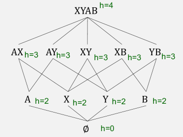
Figure 5: A lattice, and the polymatroid from [ZY98] defined on the lattice.

As a final comment, we note that it is instructive to check directly that the polymatroid in Fig. 5 fails to satisfy the copy lemma, without using Zhang and Yeung’s inequality; we provide a direct proof in Appendix .2.

Group-theoretic characterization of information inequalities Chan and Yeung [CY02] described an elegant characterization of information inequalities in terms of group inequalities. Given a finite group $G$ and a subgroup $G_{1}\subseteq G$, a left coset is a set of the form $aG_{1}$, for some $a\in G$. By Lagrange’s theorem, the set of left cosets, denoted $G/G_{1}$, forms a partition of $G$, and $|G/G_{1}|=|G|/|G_{1}|$. Fix $n$ subgroups $G_{1},\ldots,G_{n}$, and consider the relational instance:

$$R= \{{(aG_{1},\ldots,aG_{n})}\mid{a\in G}\}$$ (34)

whose set of attributes we identify, as usual, with $\bm{X}=\{X_{1},\ldots,X_{n}\}$. Notice that $|R|=|G|/|\bigcap_{i=1,n}G_{i}|$. The entropic vector $\bm{h}$ associated to the relation $R$ (Def. 4.1) is called a group realizable entropic vector, and the set of group realizable entropic vectors is denoted by $\Upsilon_{n}\subseteq\Gamma_{n}^{*}$, see Fig. 3. One can check that, for any subset of variables $\bm{U}\subseteq\bm{X}$, $h(\bm{U})=\log|G|/|\bigcap_{X_{i}\in\bm{U}}G_{i}|$. The following was proven in [CY02]:

Theorem 5.9.

For any $\bm{h}\in\Gamma_{n}^{*}$ there exists a sequence $\bm{h}^{(r)}\in\Upsilon_{n}$, such that $\lim_{r\rightarrow\infty}\frac{1}{r}\bm{h}^{(r)}=\bm{h}$.

It follows easily from the original proof that, if $\bm{h}$ satisfies a set of functional dependencies, then so do all functions $\bm{h}^{(r)}$, for $r\geq 0$; for completeness, we will include the argument in Appendix .3.

Open Problems Characterizing the valid entropic information inequalities is a major open problem. Matús [Mat07] proved that, for $n\geq 4$, there are infinitely many independent non-Shannon inequalities. Currently, the only techniques known for proving such inequalities consists of repeated applications of Shannon inequalities and the Copy Lemma.

A related open problem is the complexity of deciding Shannon inequalities: what is the complexity of checking $\Gamma_{n}\models\bm{c}\cdot\bm{h}\geq 0$, as a function of $||\bm{c}||_{1}$? It is implicit in the proof of Theorem 5.2 that this can be decided in time exponential in $n$, but the complexity in terms of $||\bm{c}||_{1}$ is open. More discussion can be found in [KKNS20]

5.2 The Entropic Bound Is Asymptotically Tight

We prove here Theorem 5.5 item (1). The plan is the following. We need to find a database $\bm{D}$ such that $\log|Q(D)|$ comes close to $\text{Log-L-Bound}_{\Gamma_{n}^{*}}(Q,\Sigma,\bm{b})$. By definition, there exists $\bm{h}\in\Gamma_{n}^{*}$ s.t. $h(\bm{X})$ is close to $\text{Log-L-Bound}_{\Gamma_{n}^{*}}(Q,\Sigma,\bm{b})$. We can’t construct a database $\bm{D}$ out of $\bm{h}$, because the probability distribution realizing $\bm{h}$ may be non-uniform, instead we use Chan and Yeung’s theorem to approximate $r\bm{h}$ by a group realizable vector $\bm{h}^{(r)}$, which is by definition associated to a relation instance. Hence, the need to amplify by the factor $r$. However, if we amplify, we don’t know how $\text{Log-L-Bound}_{\Gamma_{n}^{*}}(Q,\Sigma,r\bm{b})$ grows. Here we use Theorem 5.4, showing that $\text{Log-L-Bound}_{\Gamma_{n}^{*}}$ and $\text{Log-U-Bound}_{\Gamma_{n}^{*}}$ are asymptotically equal, then use the fact that $\text{Log-U-Bound}_{\Gamma_{n}^{*}}$ is linear, see Eq. (26). We give the details next.

By Corollary 4.8, for all $k\in\mathbb{N}$:

$$\frac{\sup_{\bm{D}:\bm{D}\models\bm{B}^{k}}\log|Q(\bm{D})|}{\text{Log-U-Bound}_{\Gamma_{n}^{*}}(Q,\Sigma,k\bm{b})}\leq 1$$

Together with Theorem 5.4 (Eq. (27)) this implies:

$$\sup_{k}\frac{\sup_{\bm{D}:\bm{D}\models\bm{B}^{k}}\log|Q(\bm{D})|}{\text{Log-L-Bound}_{\Gamma_{n}^{*}}(Q,\Sigma,k\bm{b})}\leq 1$$

To prove equality, it suffices to show that, $\forall\varepsilon>0$, $\exists k\in\mathbb{N}$ such that:

$$\log|Q(\bm{D})|\geq (1-\varepsilon)^{4}\text{Log-L-Bound}_{\Gamma_{n}^{*}}(Q,\Sigma,k\bm{b})$$ (35)

Let $U\stackrel{{\scriptstyle\text{def}}}{{=}}\text{Log-U-Bound}_{\Gamma_{n}^{*}}(Q,\Sigma,\bm{b})$. We will assume that $\text{Log-U-Bound}_{\Gamma_{n}^{*}}(Q,\Sigma,\bm{b})$ is finite; otherwise, we let $U$ be an arbitrarily large number and the proof below requires only minor adjustments, which we omit. We will assume w.l.o.g. that $U>0$. Recall that $\text{Log-U-Bound}_{\Gamma_{n}^{*}}$ is linear (26). We prove:

Claim 1.

For all $\varepsilon>0$, there exists $k\in\mathbb{N}$, and a database $\bm{D}$ such that $\bm{D}\models(\Sigma,\bm{B}^{k})$ and $\log|Q(\bm{D})|\geq(1-\varepsilon)^{4}kU$

Eq. (35) follows from $kU=\text{Log-U-Bound}_{\Gamma_{n}^{*}}(Q,\Sigma,k\bm{b})\geq\text{Log-L-Bound}_{\Gamma_{n}^{*}}(Q,\Sigma,k\bm{b})$. It remains to prove Claim 1. Since $\text{Log-L-Bound}_{\Gamma_{n}^{*}}$ and $\text{Log-U-Bound}_{\Gamma_{n}^{*}}$ are asymptotically equal (27), there exists $k_{0}\in\mathbb{N}$ such that

$$\text{Log-L-Bound}_{\Gamma_{n}^{*}}(Q,\Sigma,k_{0}\bm{b})\geq$$

$$\geq(1-\varepsilon)\text{Log-U-Bound}_{\Gamma_{n}^{*}}(Q,\Sigma,k_{0}\bm{b})=(1-\varepsilon)k_{0}U$$ (36)

By the definition of $\text{Log-L-Bound}_{\Gamma_{n}^{*}}(Q,\Sigma,k_{0}\bm{b})$ in (24), there exists $\bm{h}\in\Gamma_{n}^{*}$ such that:

$$h(\bm{X})\geq (1-\varepsilon)\text{Log-L-Bound}_{\Gamma_{n}^{*}}(Q,\Sigma,k_{0}\bm{b})\geq(1-\varepsilon)^{2}k_{0}U$$

$$h(\sigma)\leq k_{0}b_{\sigma},\ \ \ \forall\sigma\in\Sigma$$

At this point we need the following Slack Lemma:

Lemma 5.10 (Slack Lemma).

For every $\bm{h}\in\Gamma_{n}^{*}$ and every $\varepsilon\in[0,1]$, there exists $k\in\mathbb{N}$ and $\bm{h}^{\prime}\in\Gamma_{n}^{*}$ such that:

$$\bm{h}^{\prime}\geq (1-\varepsilon)k\bm{h}$$

$$\forall\bm{U},\bm{V}\subseteq\bm{X}:\ \ h^{\prime}(\bm{V}|\bm{U})\leq (1-\varepsilon/2)kh(\bm{V}|\bm{U})$$

Proof.

Assume w.l.o.g. that $\varepsilon>0$, and set $k\stackrel{{\scriptstyle\text{def}}}{{=}}\lceil{\frac{1}{\varepsilon}}\rceil$ and $\bm{h}^{\prime}\stackrel{{\scriptstyle\text{def}}}{{=}}(k-1)\bm{h}$. Then $\frac{1}{\varepsilon}\leq k\leq 1+\frac{1}{\varepsilon}\leq\frac{2}{\varepsilon}$ which implies $\varepsilon/2\leq\frac{1}{k}\leq\varepsilon$. We have:

$$\bm{h}^{\prime}= \left(1-\frac{1}{k}\right)k\bm{h}\geq(1-\varepsilon)k\bm{h}$$

$$\bm{h}^{\prime}(\bm{V}|\bm{U})= \left(1-\frac{1}{k}\right)k\bm{h}(\bm{V}|\bm{U})\leq(1-\varepsilon/2)kh^{\prime}(\bm{V}|\bm{U})$$

∎

We apply the Slack Lemma to $\bm{h}$ and obtain a number $k_{1}$ and an entropic vector $\bm{h}^{\prime}$ such that:

$$h^{\prime}(\bm{X})\geq (1-\varepsilon)k_{1}h(\bm{X})\geq(1-\varepsilon)^{3}k_{0}k_{1}U$$ (37)

$$h^{\prime}(\sigma)\leq (1-\varepsilon/2)k_{1}h(\sigma)\leq(1-\varepsilon/2)k_{0}k_{1}b_{\sigma},\ \forall\sigma\in\Sigma$$

Let $g\stackrel{{\scriptstyle\text{def}}}{{=}}\min_{\bm{U},\bm{V}\subseteq\bm{X}:h^{\prime}(\bm{V}|\bm{U})>0}h^{\prime}(\bm{V}|\bm{U})$ be the smallest non-zero value of $h^{\prime}(\bm{V}|\bm{U})$. By Chan and Yeung’s theorem 5.9, there exists a group realizable entropic vector $\bm{h}^{(r)}$ that satisfies all the FDs satisfied by $\bm{h}^{\prime}$, and $||\bm{h}^{\prime}-\frac{1}{r}\bm{h}^{(r)}||_{\infty}\leq\varepsilon g/4$. Since $U>0$ we have $h^{\prime}(\bm{X})>0$ hence $h^{\prime}(\bm{X})\geq g$ and we derive from (37):

$$\frac{1}{r}h^{(r)}(\bm{X})\geq h^{\prime}(\bm{X})-\varepsilon g/4\geq(1-\varepsilon/4)h^{\prime}(\bm{X})$$

$$\geq (1-\varepsilon)^{4}k_{0}k_{1}U$$

On the other hand, $\frac{1}{r}h^{(r)}(\bm{V}|\bm{U})\leq h(\bm{V}|\bm{U})+\varepsilon g/2$, for all sets $\bm{U},\bm{V}$. We use $\bm{h}^{\prime}\models(1-\varepsilon/2)k_{0}k_{1}\bm{b}$ to prove $\bm{h}^{(r)}\models rk_{0}k_{1}\bm{b}$. Consider a statistics $\sigma\in\Sigma$. If $h^{\prime}(\sigma)=0$, then $\bm{h}^{\prime}$ satisfies the FD $\sigma$, and therefore $\bm{h}^{(r)}$ also satisfies this FD, thus $h^{(r)}(\sigma)=0\leq k_{0}k_{1}b_{\sigma}$. If $h^{\prime}(\sigma)>0$ then $h^{\prime}(\sigma)\geq g$ and the claim follows from:

$$\frac{1}{r}h^{(r)}(\sigma)\leq h^{\prime}(\sigma)+\varepsilon g/2$$

$$\leq h^{\prime}(\sigma)+(\varepsilon/2)h^{\prime}(\sigma)=(1+\varepsilon/2)h^{\prime}(\sigma)$$

$$\leq (1+\varepsilon/2)(1-\varepsilon/2)k_{0}k_{1}b_{\sigma}\leq k_{0}k_{1}b_{\sigma}$$

So far, we have:

$$h^{(r)}(\bm{X})\geq (1-\varepsilon)^{4}rk_{0}k_{1}U \bm{h}^{(r)}\models rk_{0}k_{1}\bm{b}$$ (38)

To complete the proof of Claim 1, we construct the database $\bm{D}$ as follows. Let the relation $R$ be the group realization of $\bm{h}^{(r)}$ (Eq. (34)). For each relation $R_{j}(\bm{Y}_{j})$, define $R_{j}^{\bm{D}}\stackrel{{\scriptstyle\text{def}}}{{=}}\Pi_{\bm{Y}_{j}}(R)$. By construction, $Q(\bm{D})=R$, and $\log|Q(\bm{D})|=h^{(r)}(\bm{X})\geq(1-\varepsilon)^{4}rk_{0}k_{1}U$ by (38). Furthermore, since $\bm{h}^{(r)}$ is group-realized, for every statistics $\sigma\in\Sigma$, with guard $R_{\sigma}$, we have $\log\texttt{deg}_{R_{\sigma}}(\sigma)=h^{(r)}(\sigma)\leq rk_{0}k_{1}b_{\sigma}$; thus, $\bm{D}\models(\Sigma,\bm{B}^{rk_{0}k_{1}})$. This implies:

$$\sup_{\bm{D}:\bm{D}\models(\Sigma,\bm{B}^{rk_{0}k_{1}})}\log|Q(\bm{D})|\geq (1-\varepsilon)^{4}rk_{0}k_{1}U$$

proving Claim 1 for $k=rk_{0}k_{1}$.

5.3 The Polymatroid Bound Is Not Asymptotically Tight

We prove now Theorem 5.5 item (2).

Proposition 5.11.

The following is a non-Shannon inequality:

$$11h (ABXYC)\leq$$ (39)

$$3h(XY)+3h(AX)+3h(AY)$$

$$+ h(BX)+h(BY)+5h(C)$$

$$+ (h(XYC|AB)+4h(BC|AXY)+h(AC|BXY))$$

$$+ (h(BXY|AC)+2h(ABY|XC)+2h(ABX|YC))$$

Proof.

Consider the following five inequalities:

$$0\leq 3h(AX)+3h(AY)-4h(AXY)-h(A)$$

$$+ h(BX)+h(BY)-h(BXY)$$

$$- h(AB)+3h(XY)-2h(X)-2h(Y)$$

$$0\leq h(A)+h(C)-h(AC)$$

$$0\leq 2(h(X)+h(C)-h(XC))$$

$$0\leq 2(h(Y)+h(C)-h(YC))$$

$$11h (ABXYC)=11h(ABXYC)$$

The first inequality holds because it is inequality Eq. (32), expanded and re-arranged. The next three inequalities are basic Shannon inequalities. The last line is an identity. A tedious but straightforward calculation shows that if we add the five (in)equalities above, then we obtain (39), proving the claim. ∎

Consider the following query, derived from inequality (39):

$$Q(A,B,X,Y,C)= R_{1}(X,Y)\wedge R_{2}(A,X)\wedge R_{3}(A,Y)$$

$$\wedge R_{4}(B,X)\wedge R_{5}(B,Y)\wedge R_{6}(C)$$

$$\wedge R_{7}(A,B,X,Y,C)$$

and the following statistics:

$$\Sigma= \{(XY),(AX),(AY),(BX),(BY),(C),$$

$$\ (XYC|AB),(BC|AXY),h(AC|BXY),$$

$$\ (BXY|AC),(ABY|XC),(ABX|YC)\}$$

$$\bm{b}= \{b_{XY}=b_{AX}=b_{AY}=b_{BX}=b_{BY}=3,b_{C}=2,$$

$$\ b_{XYC|AB}=b_{BC|AXY}=b_{AC|BXY}=0,$$

$$\ b_{(BXY|AC)}=b_{ABY|XC}=b_{ABX|YC}=0\}$$

In other words, we are given the cardinalities of $R_{1},\ldots,R_{6}$, but are not given the cardinality of $R_{7}$, instead we are told that it satisfies the 6 FD’s corresponding to the 6 conditional terms in inequality (39). Consider any scale factor $k>0$, and the scaled log-statistics $k\bm{b}$. Inequality (39) and the definition (22) imply:

$$\text{Log-U-Bound}_{\Gamma_{n}^{*}}(Q,\Sigma,k\bm{b})\leq$$

$$\ \ k\frac{3b_{XY}+3b_{AX}+3b_{AY}+b_{BX}+b_{BY}+5b_{C}}{11}=\frac{43k}{11}$$

By Corollary 4.8, for any database $\bm{D}$, if $\bm{D}\models(\Sigma,\bm{B}^{k})$ then:

$$\log|Q(\bm{D})|\leq \frac{43k}{11}$$

On the other hand, consider the polymatroid $k\bm{h}$, where $\bm{h}$ is the polymatroid in Fig. 6. Since $h(ABXYC)=4$ and $\bm{h}\models(\Sigma,\bm{b})$, it follows that $kh(ABXYC)=4k$, and $k\bm{h}\models k\bm{b}$, therefore:

$$\frac{\sup_{\bm{D}:\bm{D}\models\bm{B}^{k}}\log|Q(\bm{D})|}{\text{Log-L-Bound}_{\Gamma_{n}}(Q,\Sigma,k\bm{b})}\leq \frac{43}{44}$$

This implies Theorem 5.5 item (2).

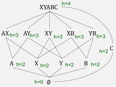
Figure 6: A polymatroid proving that the polymatroid bound is not tight.

6 Simple Inequalities

We have a dilemma: the entropic bound is asymptotically tight, but it is open whether it is computable, while the polymatroid bound is computable, but is provably not tight in general. We show in this section that, under a reasonable syntactic restriction on the statistics $\Sigma$, these two bounds are equal. We do this by describing a similar syntactic restriction for information inequalities, which we call simple inequalities. In that case validity over entropic functions coincides with validity over polymatroids, and we recover the stronger notion of tightness that we had for the AGM bound.

6.1 Background: Subclasses of Polymatroids

A polymatroid $\bm{h}$ is called modular if the submodularity inequality (15) is an equality. Equivalently, $\bm{h}$ is modular if $\bm{h}\geq 0$ and for every subset $\alpha\subseteq[n]$, $h(\bm{X}_{\alpha})=\sum_{i\in\alpha}h(X_{i})$. We will denote by $M_{n}$ the set of modular polymatroids, see Fig. 3. For each $i=1,n$, we call the function $\bm{h}^{X_{i}}$ in Fig. 4 a basic modular function; recall that $h^{X_{i}}(\bm{U})=1$ when $X_{i}\in\bm{U}$ and $=0$ otherwise. The following holds:

Proposition 6.1.

(1) A function $\bm{h}$ is modular iff it is a positive linear combination of basic modular functions, $\bm{h}=\sum_{i}a_{i}\bm{h}^{X_{i}}$, where $a_{i}\geq 0$ for all $i$. (2) Every modular function is entropic.

Proof.

Item (1) is straightforward, but item (2) requires some thought. It suffices to prove that $a\bm{h}^{X_{i}}$ is entropic for all real numbers $a\geq 0$. For that purpose we need to describe one random variable $X_{i}$, whose entropy is $h(X_{i})=a$. Let $N$ be a natural number such that $\log N\geq a$, and consider the uniform probability space where $X_{i}$ has $N$ outcomes with the same probabilities, $p_{i}=1/N$, $i=1,N$. Replace $p_{1}$ by $p_{1}+\theta$, and replace each $p_{j}$ with $j>1$ by $p_{j}-\theta/(N-1)$, for $\theta\in[0,1-\frac{1}{N}]$. When $\theta=0$ then the distribution is uniform and $h(X_{j})=\log N$; when $\theta=1-\frac{1}{N}$ then the distribution is deterministic, $p_{1}=1,p_{2}=\cdots=p_{N}=0$, and $h(X_{j})=0$. By continuity, there exists some $\theta$ where $h(X_{j})=a$. ∎

Fix a set of variables $\bm{W}\subseteq\bm{X}$. The step function at $\bm{W}$ is:

$$h_{\bm{W}}(\bm{U})\stackrel{{\scriptstyle\text{def}}}{{=}} \begin{cases}0&\mbox{if $\bm{U}\subseteq\bm{W}$}\\ 1&\mbox{otherwise}\end{cases}$$ (40)

There are $2^{n}-1$ non-zero step functions (since $\bm{h}_{\bm{X}}=0$). $\bm{h}_{\bm{W}}$ is the entropy of the (uniform distribution of the) following relation with 2 tuples:

$$R_{\bm{W}}\stackrel{{\scriptstyle\text{def}}}{{=}}R^{\bm{X}-\bm{W}}\stackrel{{\scriptstyle\text{def}}}{{=}} \ \ \ \ \ \begin{array}[]{|cc|c}\cline{1-2}\cr\bm{W}&\bm{X}-\bm{W}&p\\ \cline{1-2}\cr 0\cdots 0&0\cdots 0&1/2\\ 0\cdots 0&1\cdots 1&1/2\\ \cline{1-2}\cr\end{array}$$ (44)

Sometimes it is convenient to use an alternative notation. For a set of variables $\bm{V}\subseteq\bm{X}$, define:

$$h^{\bm{V}}(\bm{U})\stackrel{{\scriptstyle\text{def}}}{{=}} \begin{cases}0&\mbox{if $\bm{U}\cap\bm{V}=\emptyset$}\\ 1&\mbox{otherwise}\end{cases}$$ (45)

Then $\bm{h}^{\bm{V}}=\bm{h}_{\bm{X}-\bm{V}}$. A basic modular function $\bm{h}^{X_{i}}$ is the same as the step function $\bm{h}^{\{X_{i}\}}$; if $|\bm{V}|\geq 2$ then $\bm{h}^{\bm{V}}$ is not modular.

Definition 6.2.

A normal polymatroid is a positive linear combination of step functions,

$$\bm{h}= \sum_{\bm{V}\subseteq\bm{X},\bm{V}\neq\emptyset}a_{\bm{V}}\bm{h}^{\bm{V}}$$ (46)

where $a_{\bm{V}}\geq 0$ for all $\bm{V}$.

We denote by $N_{n}$ the set of normal polymatroids, see Fig. 3. Normal polymatroids are the same as polymatroids with a non-negative I-measure described in [Yeu08, KKNS21].

Proposition 6.3.

The $2^{n}-1$ non-zero step functions $\bm{h}^{\bm{V}}$, $\bm{V}\neq\emptyset$ form a basis of the vector space $\{{\bm{h}\in\mathbb{R}^{2^{[n]}}}\mid{h(\emptyset)=0}\}$. More precisely, every such vector $\bm{h}$ satisfies $\bm{h}=\sum_{\bm{V}}a_{\bm{V}}\bm{h}^{\bm{V}}$, where:

$$a_{\bm{U}}\stackrel{{\scriptstyle\text{def}}}{{=}} -\sum_{\bm{V}\subseteq\bm{U}}(-1)^{|\bm{V}|}h(\bm{V}|\bm{X}-\bm{U})$$ (47)

The proof follows by solving the following system of linear equations with unknowns $a_{\bm{V}}$:

$$\forall\bm{U}\neq\emptyset:\ \ \ h(\bm{U})= \sum_{\bm{V}:\bm{V}\cap\bm{U}\neq\emptyset}a_{\bm{V}}$$ (48)

The solution is obtained by using Möbius’ inversion formula (we prove this in Appendix .4) and consists of the expression (47). Expression (47) is called conditional interaction information, and denoted by $I(X_{i_{1}};X_{i_{2}};\cdots|\bm{X}-\bm{U})$, where $\bm{U}=\{X_{i_{1}},X_{i_{2}},\ldots\}$. The following holds (the proof is immediate and omitted):

Proposition 6.4.

(1) A function $\bm{h}$ is a normal polymatroid iff, for every set $\bm{U}\subseteq\bm{X}$, $\bm{U}\neq 0$, the conditional interaction information (47) is $\geq 0$. (2) Every normal polymatroid is entropic.

Example 6.5.

The parity function $\bm{h}$ Fig. 2 is the simplest example of a polymatroid that is not normal. The coefficients can be derived using (47), or, we can check directly that:

$$\bm{h}= \bm{h}^{X,Y}+\bm{h}^{X,Z}+\bm{h}^{Y,Z}-\bm{h}^{X,Y,Z}$$

The coefficient of $\bm{h}^{X,Y,Z}$ is negative, hence $\bm{h}$ is not normal.

6.2 Special Inequalities

We describe here a class of information inequalities, called simple inequalities, were $\Gamma_{n}^{*}$-validity coincides with $\Gamma_{n}$-validity. The modular and normal polymatroids turn out to be the key tools to study these inequalities.

The following is sometimes referred in the literature as the modularization lemma:

Lemma 6.6.

For any polymatroid $\bm{h}$ there exists a modular polymatroid $\bm{h}^{\prime}$ such that (a) $\bm{h}^{\prime}\leq\bm{h}$ and (b) $\bm{h}^{\prime}(\bm{X})=\bm{h}(\bm{X})$.

Proof.

Order the variables arbitrarily $X_{1},\ldots,X_{n}$ and define $h^{\prime}(X_{i})\stackrel{{\scriptstyle\text{def}}}{{=}}h(X_{i}|\bm{X}_{[1:i-1]})$, where $\bm{X}_{[1:i-1]}\stackrel{{\scriptstyle\text{def}}}{{=}}\{X_{1},\ldots,X_{i-1}\}$. We check condition (a): for $\alpha\subseteq[n]$,

$$h^{\prime}(\bm{X}_{\alpha})= \sum_{i\in\alpha}h(X_{i}|\bm{X}_{[1:i-1]})$$

$$\leq \sum_{i\in\alpha}h(X_{i}|\bm{X}_{[1:i-1]\cap\alpha})=h(\bm{X}_{\alpha})$$

We check (b): $h^{\prime}(\bm{X})=\sum_{i=1,n}h(X_{i}|\bm{X}_{[1:i-1]})=h(\bm{X})$. ∎

The modularization lemma gives us an alternative, and more general proof of Theorem 4.10:

Corollary 6.7.

Consider an inequality of the form $\sum_{i}w_{i}h(\bm{V}_{i})\geq h(\bm{X})$, where $w_{i}\geq 0$ and $\bm{V}_{i}$ are subsets of $\bm{X}$. The following conditions are equivalent:

1. The inequality is valid for polymatroids.

2. The inequality is valid for entropic functions.

3. The inequality is valid for modular functions.

Proof.

The implications 1 $\Rightarrow$ 2 $\Rightarrow$ 3 are immediate. We prove 3 $\Rightarrow$ 1, by contradiction: if the inequality fails on some polymatroid $\bm{h}$, $\sum_{i}w_{i}h(\bm{V}_{i})<h(\bm{X})$, and $\bm{h}^{\prime}$ is the modular function in Lemma 6.6, then, $\sum_{i}w_{i}h^{\prime}(\bm{V}_{i})\leq\sum_{i}w_{i}h(\bm{V}_{i})<h(\bm{X})=h^{\prime}(\bm{X})$ contradicting 3. ∎

We prove in Appendix .5 the following extension of the Modularization Lemma:

Lemma 6.8.

For any polymatroid $\bm{h}$ there exists a normal polymatroid $\bm{h}^{\prime}$ such that (a) $\bm{h}^{\prime}\leq\bm{h}$, (b) $h^{\prime}(\bm{X})=h(\bm{X})$, and (c) $h^{\prime}(X_{i})=h(X_{i})$ for every variable $X_{i}\in\bm{X}$.

Definition 6.9.

We call a set of statistics $\Sigma$ simple if, for all $(\bm{V}|\bm{U})\in\Sigma$, $|\bm{U}|\leq 1$. A simple information inequality is a $\Sigma$-inequality where $\Sigma$ is simple:

$$\sum_{\sigma\in\Sigma}w_{\sigma}h(\Sigma)\geq h(\bm{X})$$ (49)

We immediately derive:

Corollary 6.10.

Given a simple inequality (49), the following are equivalent:

1. The inequality is valid for polymatroids.

2. The inequality is valid for entropic functions.

3. The inequality is valid for normal polymatroids

The proof is identical to that of Corollary 6.7 and omitted.

6.3 Special Databases

When the statistics $\Sigma$ are simple, then we show here that the polymatroid and the entropic bound coincide. We also show that the bound is tight, using a similar notion of tightness as in the AGM bound, where the ratio between the lower and upper bound depends only on the query; also, there is no need to amplify the statistics values. Moreover, like in the AGM bound, the worst-case database instance has a special structure, which we call a normal database. We start by showing:

Theorem 6.11.

If $\Sigma$ is simple, then:

$$\text{Log-U-Bound}_{N_{n}}(Q,\Sigma,\bm{b})=$$

$$\ \ \ =\text{Log-U-Bound}_{\Gamma_{n}^{*}}(Q,\Sigma,\bm{b})=\text{Log-U-Bound}_{\Gamma_{n}}(Q,\Sigma,\bm{b})$$

Proof.

Since $N_{n}\subseteq\Gamma_{n}^{*}\subseteq\Gamma_{n}$ we have inequalities above: $\cdots\leq\cdots\leq\cdots$ Corollary 6.10 implies $\text{Log-U-Bound}_{N_{n}}(Q,\Sigma,\bm{b})=\text{Log-U-Bound}_{\Gamma_{n}}(Q,\Sigma,\bm{b})$, hence all three quantities are equal. ∎

We describe now normal relational instances, and normal databases. Start with a single relation $R(\bm{X})$ with $n$ attributes $\bm{X}$. Recall that an instance $R$ is a product relation if $R=S_{1}\times\cdots\times S_{n}$, for $n$ sets $S_{1},\ldots,S_{n}$: the worst-case instance of the AGM bound consisted of product relations. We generalize this concept:

Definition 6.12.

A relation instance $T$ with $n$ attributes is a normal relation if there exists $m$ finite sets $S_{1},\ldots,S_{m}$ and a function $\psi:[n]\rightarrow 2^{[m]}$ such that

$$T= \{{(\bm{s}_{\psi(1)},\bm{s}_{\psi(2)},\ldots,\bm{s}_{\psi(n)})}\mid{\bm{s}\in S_{1}\times\cdots\times S_{m}}\}$$

In a normal relation the values of an attribute can be tuples themselves. Every product relation is a normal relation, but not vice versa. A database instance is normal if each of its relations is normal. A basic normal relation of size $N$ is the following:

$$T^{\bm{V}}_{N}\stackrel{{\scriptstyle\text{def}}}{{=}} \{{(k\cdot\bm{1}_{X_{1}\in\bm{V}},\cdots,k\cdot\bm{1}_{X_{n}\in\bm{V}})}\mid{k=0,N-1}\}$$ (50)

Here $\bm{1}_{X_{i}\in\bm{V}}$ is an indicator variable that is 1 when $X_{i}\in\bm{V}$ and 0 otherwise; thus, if an attribute $X_{i}$ is in $\bm{V}$ then it takes the values $0,1,\ldots,N-1$ in the relation $T^{\bm{V}}_{N}$, otherwise it has constant values 0. The entropic vector of $T^{\bm{V}}_{N}$ is $(\log N)\bm{h}^{\bm{V}}$. In particular, the relation $R^{\bm{V}}$ in (44) is $T^{\bm{V}}_{2}$.

Example 6.13.

We give three examples of normal relations with $n=3$ attributes:

$$A= \{{(i,j,k)}\mid{i,j,k\in[0:N-1]}\}$$ product relation

$$B= \{{(i,i,i)}\mid{i\in[0:N-1]}\},$$ normal relation

$$C= \{{(i,(i,j),j)}\mid{i,j\in[0:N-1]}\}$$ normal relation

Their cardinalities are $|A|=N^{3}$, $|B|=N$, $|C|=N^{2}$. We also notice:

$$A= T^{X}_{N}\otimes T^{Y}_{N}\otimes T^{Z}_{N} B= T^{XYZ}_{N} C= T^{X,Y}_{N}\otimes T^{Y,Z}_{N}$$

We prove that the lower bound for simple statistics is tight.

Theorem 6.14.

Let $\Sigma$ be a set of simple statistics for a query $Q$ and let $\bm{B}$ be statistics values. Then there exists a worst-case instance $\bm{D}$ such that $|Q(\bm{D})|\geq\frac{1}{2^{2^{n}-1}}\text{U-Bound}_{\Gamma_{n}^{*}}(Q,\Sigma,\bm{B})$.

Proof.

We use the following, whose proof is immediate:

Proposition 6.15.

Let $R(\bm{X})$, $R^{\prime}(\bm{X})$ be relations over the same attributes $\bm{X}$.

• If $R,R^{\prime}$ are normal relations, then $R\otimes R^{\prime}$ is normal.

• $\texttt{deg}_{R\otimes R^{\prime}}(\sigma)=\texttt{deg}_{R}(\sigma)\cdot\texttt{deg}_{R^{\prime}}(\sigma)$, for all $\sigma=(\bm{V}|\bm{U})$.

Denote by $U\stackrel{{\scriptstyle\text{def}}}{{=}}\text{U-Bound}_{\Gamma_{n}^{*}}(Q,\Sigma,\bm{B})$, $\bm{b}\stackrel{{\scriptstyle\text{def}}}{{=}}\log\bm{B}$, then $\log U=\text{Log-U-Bound}_{N_{n}}(Q,\Sigma,\bm{b})=\text{Log-L-Bound}_{N_{n}}(Q,\Sigma,\bm{b})$, by Theorem 6.11 and Theorem 5.2 respectively. Let $\bm{h}^{*}\in N_{n}$ be the optimal solution to the linear program defining $\text{Log-L-Bound}_{N_{n}}(Q,\Sigma,\bm{b})$ (see Theorem 5.2), then $\bm{h}^{*}\models(\Sigma,\bm{b})$ and $h^{*}(\bm{X})=\log U$. Since $\bm{h}^{*}$ is normal, it can be written as:

$$\bm{h}^{*}= \sum_{\bm{V}\neq\emptyset}a_{\bm{V}}\bm{h}^{\bm{V}},\ \ \ \ a_{\bm{V}}\geq 0$$

Then, $\log U=h^{*}(\bm{X})=\sum_{\bm{V}\neq\emptyset}a_{\bm{V}}$, and $U=\prod_{\bm{V}}2^{a_{\bm{V}}}$.

For each set $\bm{V}$, $\emptyset\neq\bm{V}\subseteq\bm{X}$ we define:

$$b_{\bm{V}}\stackrel{{\scriptstyle\text{def}}}{{=}}\lfloor{2^{a_{\bm{V}}}}\rfloor,\ \ \ P^{\bm{V}}\stackrel{{\scriptstyle\text{def}}}{{=}} T^{\bm{V}}_{b_{\bm{V}}}$$ basic normal relation (50)

$$R\stackrel{{\scriptstyle\text{def}}}{{=}} \bigotimes_{\bm{V}}P^{\bm{V}}$$ normal relation

Define the worst-case instance as $\bm{D}=(R_{1}^{D},\ldots,R_{m}^{D})$, where $R_{j}^{D}=\Pi_{\bm{Y}_{j}}(R)$. We first check that $\bm{D}$ satisfies the constraints, and for that let $\sigma\in\Sigma$ have witness $R_{\sigma}$, then:

$$\log \texttt{deg}_{R_{\sigma}}(\sigma)=\log\texttt{deg}_{R}(\sigma)=\sum_{\bm{V}}\log\texttt{deg}_{P^{\bm{V}}}(\sigma)$$

$$= \sum_{\bm{V}}(\log b_{\bm{V}})h^{\bm{V}}(\sigma)\leq\sum_{\bm{V}}a_{\bm{V}}h^{\bm{V}}(\sigma)=h^{*}(\sigma)\leq b_{\sigma}$$

Finally, we check the query’s output size:

$$\log |Q(\bm{D})|=\log|R|=\log\prod_{\bm{V}}|P^{\bm{V}}|=\sum_{\bm{V}}(\log b_{\bm{V}})h^{\bm{V}}(\bm{X})$$

Since $h^{\bm{V}}(\bm{X})=1$, this implies $|Q(\bm{D})|=\prod_{\bm{V}}b_{\bm{V}}=\prod_{\bm{V}}\lfloor{2^{a_{\bm{V}}}}\rfloor\geq\frac{1}{2^{2^{n}-1}}U$, because $\lfloor{2^{a_{\bm{V}}}}\rfloor\geq\frac{1}{2}2^{a_{\bm{V}}}$. ∎

The reader may want to check the analogy with the worst-case instance of the AGM bound: the optimal solution $\bm{v}^{*}$ there became here $\bm{h}^{*}$, and the domain $V_{i}=[\lfloor{2^{v_{i}^{*}}}\rfloor]$ defined for the variable $X_{i}$ became here the normal relation $P^{\bm{V}}$. As before, we constructed the worst-case instance $\bm{D}$ without amplifying the statistics, and $|Q(\bm{D})|$ is within a constant, which depends only on the query, of $\text{U-Bound}_{\Gamma_{n}^{*}}(Q,\Sigma,\bm{B})$.

Discussion The restriction to simple statistics occurs naturally in many applications. Databases are often designed with simple keys (consisting of a single attribute), and applications that use degrees often consider only simple degrees. The restriction to simple statistics is often acceptable.

It remains open where one can extend this definition to richer classes of statistics, or inequalities, while still preserving the property that validity for entropic vectors is the same as validity for polymatroids. The set of statistics in Example 4.9 is not “simple”, yet the entropic bound coincides with the polymatroid bound. This (and other examples) suggests that other non-trivial syntactic classes may exist where these two bounds agree.

7 Query Evaluation

The query evaluation problem is: given a conjunctive query $Q$, evaluate it on a (usually large) database $\bm{D}$. In this paper we consider only the data complexity, where the query is fixed, and the runtime is given as a function of the statistics of $\bm{D}$. Database systems compute queries using a sequence of binary joins, of the form $C(X,Y,Z)=A(X,Y)\wedge B(Y,Z)$, which are written as $C=A\bowtie B$. Assuming all relations are pre-sorted, the time complexity of the join is $\tilde{O}(|A|+|B|+|A\bowtie B|)$. A semi-join, denoted $C=A\ltimes B$, is a join followed by the projection on the attributes of the first relation, meaning $C(X,Y)=\exists Z(A(X,Y)\wedge B(Y,Z))$. A semijoin can be computed in time $\tilde{O}(|A|)$.

A Worst Case Optimal Join (WCOJ) is an algorithm that evaluates $Q$ in time no larger than its theoretical upper bound. A sequence of binary joins is usually not a WCOJ, because intermediate results may be larger than the theoretical upper bound of the query. For example the upper bound for the triangle query in Example 3.2 is $N^{3/2}$, but if we evaluate it as $(R\bowtie S)\bowtie T$, the join $R\bowtie S$ can have size $N^{2}$.

Any WCOJ algorithm represents an indirect proof of the query’s upper bound, since the size of the output cannot exceed the time complexity of the algorithm. For example, if we are given an algorithm for the triangle query, together with a proof that its runtime is $\tilde{O}(N^{3/2})$, then we have a proof that the size of the output is also $\tilde{O}(N^{3/2})$. This means that proving an upper bound on the query’s output is inevitable for designing a WCOJ. We show in this section that one can proceed in reverse: given a proof of the upper bound, convert it into a WCOJ. We call this paradigm From Proofs to Algorithms. Thus, the question to ask in designing a WCOJ algorithm is: how do we prove an upper bound on the query’s output? And how do we convert it into an algorithm?

7.1 Generic Join

Consider the setting of the AGM bound: we are given only cardinality statistics on the base relations. In that case, a proof of the upper bound is a proof of $\sum_{j}w_{j}h(\bm{Y}_{j})\geq h(\bm{X})$, since it implies $|Q|\leq\prod_{j}|R_{j}|^{w_{j}}$. We gave a proof of this inequality in Theorem 4.10; the proof consists of conditioning on the last variable $X_{n}$, then applying induction on the remaining variables. We convert that proof into an algorithm: iterate $X_{n}$ over its domain, and compute recursively the residual query. This algorithm is called Generic Join, or GJ, and was introduced by Ngo, Ré, and Rudra [NRR13]. We describe it in detail next.

Fix a full conjunctive query with variables $\bm{X}$, which we write as $Q={{{\Join}}}_{j=1,m}R_{j}$. As usual, $\bm{Y}_{j}$ are the variables of $R_{j}$. Generic Join computes $Q$ as follows:

• Let $X_{n}$ be an arbitrary variable.

• Partition the set of indices $j$ into $J_{0}$ and $J_{1}$:
  $J_{0}\stackrel{{\scriptstyle\text{def}}}{{=}}\{{j}\mid{X_{n}\not\in\bm{Y}_{j}}\}$, $J_{1}\stackrel{{\scriptstyle\text{def}}}{{=}}\{{j}\mid{X_{n}\in\bm{Y}_{j}}\}$.

• Compute the set $D=\bigcap_{j\in J_{1}}\Pi_{X_{n}}(R_{j})$.

• For each value $x\in D$, do:

  • Compute $R_{j}[x]:=\Pi_{\bm{Y}_{j}-X_{n}}(\sigma_{X_{n}=x}(R_{j}))$, for $j\in J_{1}$.

  • Denote $R_{j}[x]:=R_{j}$ for $j\in J_{0}$.

  • Compute the residual query ${{{\Join}}}_{j=1,m}R_{j}[x]$.

We invite the reader to check how the algorithm can be “read off” the proof of Theorem 4.10. To compute the runtime of the algorithm, assume that the relations are given in listing representation, sorted lexicographically using the attribute order $X_{n},X_{n-1},\ldots,X_{1}$. Then, the runtime, $T_{n}$, is:

$$T_{n}(R_{1},\ldots,R_{m})= T_{\text{intersection}}+\sum_{x}T_{n-1}(R_{1}[x],\ldots,R_{m}[x])$$

By induction hypothesis:

$$T_{n-1}(R_{1}[x],\ldots,R_{m}[x])= \tilde{O}\left(\prod_{j}|R_{j}[x]|^{w_{j}}\right)$$

which leads to:

$$T_{n} =T_{\text{intersection}}+\tilde{O}\left(\prod_{j\in J_{0}}|R_{j}|^{w_{j}}\sum_{x}\prod_{j\in J_{1}}|R_{j}[x]|^{w_{j}}\right)$$

$$\leq T_{\text{intersection}}+\tilde{O}\left(\prod_{j\in J_{0}}|R_{j}|^{w_{j}}\prod_{j\in J_{1}}\left(\sum_{x}|R_{j}[x]|\right)^{w_{j}}\right)$$

$$= T_{\text{intersection}}+\tilde{O}\left(\prod_{j}|R_{j}|^{w_{j}}\right)$$

We used Hölder’s inequality in Fig. 1 (since $\sum_{j\in J_{1}}w_{j}\geq 1$, because $X_{n}$ is covered), and the fact that $\sum_{x}|R_{j}[x]|=|R_{j}|$ for $j\in J_{1}$. The crux of the algorithm is the intersection: its runtime should not exceed $\prod_{j}|R_{j}|^{w_{j}}$, and for that it suffices to iterate over the smallest set $\Pi_{X_{n}}(R_{j})$, and probe in the others: the runtime is $\tilde{O}(\min_{j\in J_{1}}|R_{j}|)\leq\tilde{O}(\prod_{j\in J_{1}}|R_{j}|^{w_{j}})$, since $\sum_{j\in J_{1}}w_{j}\geq 1$.

Example 7.1.

Using the variable order $X,Y,Z$, GJ computes the triangle query $R(X,Y)\wedge S(Y,Z)\wedge T(Z,X)$ as follows:

$$\texttt{For }x\in\Pi_{X}(R)\cap\Pi_{X}(T)\texttt{ do:}$$

$$\ \ \ \texttt{For }y\in\Pi_{Y}(R[X=x])\cap\Pi_{Y}(S)\texttt{ do:}$$

$$\ \ \ \ \ \texttt{For }z\in\Pi_{Z}(S[Y=y])\cap\Pi_{Z}(T[X=x])\texttt{ do:}$$

$$\ \ \ \ \ \ \ \texttt{output}(x,y,z)$$

The choice of algorithm for computing the intersection is critical for GJ. To see this, consider the simplest query, $Q(X)=R(X)\wedge S(X)$, that is an intersection. The AGM bound is $\min(|R|,|S|)$, corresponding to the edge covers $(1,0)$ and $(0,1)$, and GJ must compute the query in time $\tilde{O}(\min(|R|,|S|))$. By assumption, $R,S$ are already sorted, but we cannot run a standard merge algorithm, since its runtime is $O(|R|+|S|)$; instead, we iterate over the smaller relation and do a binary search in the larger.

Because of its simplicity and ease of implementation, GJ is the poster child of WCOJ algorithms. One remarkable property of GJ is that its runtime is always bounded by the AGM bound, no matter what variable order we choose. Before GJ, Veldhuizen [Vel14] described an algorithm called Leapfrog Triejoin (LFTJ), which uses a similar logic as GJ, but also specifies in the details of the required trie data structure. Several implementations of GJ/LFTJ exists today [SOC16, AtCG⁺15, FBS⁺20, MKS21, WWS23].

7.2 The Heavy/Light Algorithm

Balister and Bollobás [BB12] provided the following alternative proof of an inequality of the form (23), which we write in an equivalent form using integer coefficients:

$$E\stackrel{{\scriptstyle\text{def}}}{{=}}\sum_{j=1,m}k_{j}h(\bm{Y}_{j})\geq k_{0}h(\bm{X})$$ (51)

where $k_{i}\in\mathbb{N}$, for $i=0,m$. View the expression $E$ as a bag of terms $h(\bm{Y}_{j})$ where each term $h(\bm{Y}_{j})$ occurs $k_{j}$ times. A compression step consists of the following:

• Choose two terms $h(\bm{U}),h(\bm{V})\in E$ such that $\bm{U}\not\subseteq\bm{V}$ and $\bm{V}\not\subseteq\bm{U}$.

• Replace $h(\bm{U})+h(\bm{V})$ with $h(\bm{U}\cup\bm{V})+h(\bm{U}\cap\bm{V})$.

Theorem 7.2.

[BB12] Any sequence of compression steps eventually leads to:

$$E= \ell_{0}h(\bm{Z}_{0})+\ell_{1}h(\bm{Z}_{1})+\cdots, \bm{Z}_{0}\supset\bm{Z}_{1}\supset\cdots$$ where (52)

Furthermore, if each variable $X_{i}$ is covered at least $k_{0}\geq 1$ times by the original expression $E$ in (51), then $\bm{Z}_{0}=\bm{X}$ and $\ell_{0}\geq k_{0}$; in particular, the inequality (51) is valid.

Proof.

Each compression step strictly increases the quantity $\sum_{h(\bm{Z})\in E}|\bm{Z}|^{2}$. To see this, write $\bm{U}=\bm{A}\cup\bm{C}$, $\bm{V}=\bm{B}\cup\bm{C}$ where $\bm{A},\bm{B},\bm{C}$ are disjoint sets, then $|\bm{U}|^{2}+|\bm{V}|^{2}=(|\bm{A}|+|\bm{C}|)^{2}+(|\bm{B}|+|\bm{C}|)^{2}$, while $|\bm{U}\cup\bm{V}|^{2}+|\bm{U}\cap\bm{V}|^{2}=(|\bm{A}|+|\bm{B}|+|\bm{C}|)^{2}+|\bm{C}|^{2}$, and the latter is strictly larger when $|\bm{A}|\cdot|\bm{B}|>0$. This quantity cannot exceed $(\sum_{j}k_{j})n^{2}$, therefore compression needs to terminate, and this happens when for any two sets in $E$ one contains the other. Then, $E$ must have the form (52). Finally, we observe that compression preserves the number of times each variable $X_{i}$ is covered by $E$, because the number of sets in $\{\bm{U},\bm{V}\}$ containing $X_{i}$ is the same as the number of sets in $\{\bm{U}\cup\bm{V},\bm{U}\cap\bm{V}\}$ containing $X_{i}$. Therefore, if each variable is covered by $E$ at least $k_{0}$ times, then $\bm{Z}_{0}=\bm{X}$ and $\ell_{0}\geq k_{0}$. ∎

Call a sequence of compression steps that converts an expression $E$ in (51) to (52) a BB-proof sequence. To derive an algorithm, we need to impose an additional restriction. Call a BB-proof sequence divergent if, after each compression step $h(\bm{U})+h(\bm{V})\rightarrow h(\bm{U}\cup\bm{V})+h(\bm{U}\cap\bm{V})$, we can split $E$ into $E^{\prime}+E^{\prime\prime}$, such that $E^{\prime}$ contains $h(\bm{U}\cup\bm{V})$ and covers every variable at least $k_{0}^{\prime}$ times, $E^{\prime\prime}$ contains $h(\bm{U}\cap\bm{V})$ and covers every variable at least $k_{0}^{\prime\prime}$ times, and $k_{0}=k_{0}^{\prime}+k_{0}^{\prime\prime}$.

We convert a divergent BB-proof sequence into an algorithm called the Heavy/Light Algorithm. Let $\bm{B}$ be the statistics values, $\bm{b}\stackrel{{\scriptstyle\text{def}}}{{=}}\log\bm{B}$, and set $B\stackrel{{\scriptstyle\text{def}}}{{=}}\max_{j}B_{j}$. Assume w.l.o.g. that the inequality $E\stackrel{{\scriptstyle\text{def}}}{{=}}\sum_{j}k_{j}h(\bm{Y}_{j})\geq k_{0}h(\bm{X})$ is optimal, meaning that $\sum_{j}(k_{j}/k_{0})b_{j}=\text{Log-U-Bound}_{\Gamma_{n}}(Q,\Sigma,\log(\bm{B}))$ (see Eq. (22)). Denote by $\bm{h}^{*}$ an optimal solution to the dual, meaning $\bm{h}^{*}\models(\Sigma,\bm{b})$ and $h^{*}(\bm{X})=\text{Log-L-Bound}_{\Gamma_{n}}(Q,\Sigma,\bm{b})$ (see Eq. (24)). These two quantities are the same by Thm. 5.2: $\sum_{j}(k_{j}/k_{0})b_{j}=h^{*}(\bm{X})$. The algorithm uses a working memory which stores, for each term $h(\bm{Z})$ in $E$, a temporary relation $S(\bm{Z})$, called the guard of $h(\bm{Z})$, and maintains the invariant: $\log|S(\bm{Z})|\leq h^{*}(\bm{Z})$. Initially, the working memory is $\{{R_{j}}\mid{k_{j}>0}\}$: by complementary slackness, if $k_{j}>0$ then the dual constraint constraint is tight, $h^{*}(\bm{Y}_{j})=b_{j}$, and the invariant holds because $\log|R_{j}|\leq\log B_{j}=b_{j}=h^{*}(\bm{Y}_{j})$.

The algorithm repeatedly processes a compression step $h(\bm{U})+h(\bm{V})\rightarrow h(\bm{U}\cup\bm{V})+h(\bm{U}\cap\bm{V})$ of the BB-sequence, as follows. If the two guards are $S(\bm{U})$ and $S^{\prime}(\bm{V})$, let $\bm{C}\stackrel{{\scriptstyle\text{def}}}{{=}}\bm{U}\cap\bm{V}$, write $\bm{U}=\bm{A}\bm{C}$, $\bm{V}=\bm{B}\bm{C}$, and define $M\stackrel{{\scriptstyle\text{def}}}{{=}}2^{h^{*}(\bm{A}|\bm{C})}$. Partition the guard $S(\bm{A}\bm{C})$ into two subsets:

$$S_{\text{light}}(\bm{A},\bm{C})= \{{(\bm{a},\bm{c})\in S}\mid{\texttt{deg}_{S}(\bm{A}|\bm{C}=\bm{c})\leq M}\}$$

$$S_{\text{heavy}}(\bm{C})= \{{\bm{c}\in\Pi_{\bm{C}}(S)}\mid{\texttt{deg}_{S}(\bm{A}|\bm{C}=\bm{c})>M}\}$$

Compute new guards using a join and a semijoin:

$$S^{\prime\prime}(\bm{A},\bm{B},\bm{C}):= S_{\text{light}}(\bm{A},\bm{C})\bowtie S^{\prime}(\bm{B},\bm{C})$$

$$S^{\prime\prime\prime}(\bm{C}):= S_{\text{heavy}}(\bm{C})\ltimes S^{\prime}(\bm{B},\bm{C})$$

The invariant holds because $|S^{\prime\prime}|\leq M\cdot|S|$ implies $\log|S^{\prime\prime}|\leq h^{*}(\bm{A}|\bm{C})+h^{*}(\bm{B}\bm{C})\leq h^{*}(\bm{A}\bm{B}\bm{C})$, and because $|S_{\text{heavy}}|\leq|S|/M$ (since every $\bm{c}\in S_{\text{heavy}}$ occurs $\geq M$ times in $S$) implies $\log|S^{\prime\prime\prime}|\leq\log|S|-\log M=h^{*}(\bm{A}\bm{C})-h^{*}(\bm{A}|\bm{C})=h^{*}(\bm{C})$. The runtime of the join and semijoin is $\leq\tilde{O}(2^{h^{*}(\bm{X})})=\tilde{O}(\text{U-Bound}_{\Gamma_{n}}(Q,\Sigma,\bm{B}))$. Next, the algorithm proceeds recursively, by processing independently $E^{\prime}$ and $E^{\prime\prime}$, semi-joins the result of $E^{\prime}$ with the relations missing from $E^{\prime}$, similarly semi-joins the result of $E^{\prime\prime}$ with the relations missing from $E^{\prime\prime}$, then returns the union of these two results. Correctness is easily checked.

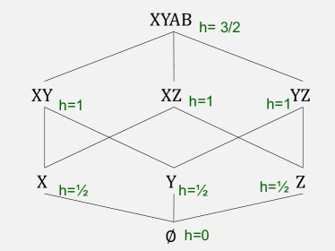
Figure 7: A simple polymatroid used in Example 7.3.

Example 7.3.

Consider the triangle query $R(X,Y)\wedge S(Y,Z)\wedge T(Z,X)$, and the following divergent proof: $\underline{h(XY)+h(YZ)}+h(ZX)\rightarrow h(XYZ)+\underline{h(Y)+h(ZX)}\rightarrow h(XYZ)+h(XYZ)$. Assume for simplicity that the three relations have the same cardinalities $|R|=|S|=|T|=B$. The optimal polymatroid is $\bm{h}^{*}\stackrel{{\scriptstyle\text{def}}}{{=}}\log B\cdot\bm{h}$, for $\bm{h}$ in Fig. 7.

The Heavy/Light Algorithm proceeds as follows. For the first compression step it partitioning $R$ into:

$$R_{\text{light}}:= \{{(x,y)}\mid{\texttt{deg}_{R}(X|Y=y)\leq 2^{h^{*}(Y|X)}=B^{1/2}}\}$$

$$R_{\text{heavy}}:= \{{y}\mid{\texttt{deg}_{R}(X|Y=y)>2^{h^{*}(Y|X)}=B^{1/2}}\}$$

then it computes:

$$\texttt{Temp}_{1}(X,Y,Z):= R_{\text{light}}(X,Y)\bowtie S(Y,Z)$$

$$\texttt{Temp}_{2}(Y):= R_{\text{heavy}}(Y)\ltimes S(Y,Z)$$

At this point the BB-proof diverged into two branches, $h(XYZ)\geq h(XYZ)$, and $h(Y)+h(ZX)\geq h(XYZ)$, and we perform a recursive call for each branch. The first branch immediately returns $\texttt{Temp}_{1}$, which we semi-join with $T$: $Q^{\prime}(X,Y,Z)=\texttt{Temp}_{1}(X,Y,Z)\ltimes T(Z,X)$. The other branch applies the second compression step which corresponds to the following join operation:

$$\texttt{Temp}_{3}(X,Y,Z):= \texttt{Temp}_{2}(Y)\times T(Z,X)$$

which we semi-join with $R$ and $S$: $Q^{\prime\prime}(X,Y,Z):=\texttt{Temp}_{3}(X,Y,Z)\ltimes R(X,Y)\ltimes S(Y,Z)$. Finally, we return the union $Q^{\prime}\cup Q^{\prime\prime}$. The reader may verify that the runtime is $\tilde{O}(B^{3/2})$.

An advantage of the Heavy/Light Algorithm over GJ is that it reuses existing join operators, which already have very efficient implementations in database systems. However, the algorithm only works for divergent BB-proofs. This raises the question: does every inequality (51) have a divergent proof? The answer is negative, as provided by the following example due to Yilei Wang [Wan22].

Example 7.4.

The following has no divergent BB-proof:

$$E=h(XYZ)+h(ZUV)+h(VWX)+h(YUW)\geq 2h(XYZUVW)$$

Assume w.l.o.g. that we start by compressing $h(XYZ)+h(ZUV)\rightarrow h(XYZUV)+h(Z)$ (by symmetry, all other choices are equivalent). Then we need to partition $E$ into $E^{\prime}+E^{\prime\prime}$. Suppose $E^{\prime}$ contains $h(Z)$; since $E^{\prime}$ covers every variable, it must contain both remaining terms $h(VWX)+h(YUW)$, which means that $E^{\prime\prime}$ can only contain $h(XYZUV)$ alone, and it does not cover $W$.

7.3 PANDA

Both Generic Join and the Heavy/Light Algorithm are restricted to cardinality statistics, in other words they only work in the framework of the AGM bound. PANDA, introduced in [KNS17], is a WCOJ algorithm that works for general statistics. While it runs in time given by the theoretical query upper bound, it also includes a polylogarithm factor in the size of the database, with a rather large exponent. We describe PANDA here at a high level, and refer the reader to [KNS17] for details.

Let $\Sigma$ be a set of statistics, and consider a $\Sigma$-inequality with integer coefficients:

$$E\stackrel{{\scriptstyle\text{def}}}{{=}}\sum_{\sigma\in\Sigma}k_{\sigma}h(\sigma)\geq k_{0}h(\bm{X})$$ (53)

A CD-proof sequence for the inequality (53) is a sequence of steps that convert the LHS to the RHS, where each step is one of the following:

• Composition: $h(\bm{U})+h(\bm{V}|\bm{U})\rightarrow h(\bm{U}\bm{V})$.

• Decomposition: $h(\bm{U}\bm{V})\rightarrow h(\bm{U})+h(\bm{V}|\bm{U})$.

• Submodularity: $h(\bm{V}|\bm{U})\rightarrow h(\bm{V}|\bm{U}\bm{W})$.

• No-Op: $h(\bm{U})\rightarrow 0$.

We say that the CD-proof sequence proves the inequality (53) if its starts from the LHS and ends with the RHS. The following was proven in [KNS17]:

Lemma 7.5.

Inequality (53) is valid for polymatroids iff it admits a CD-proof sequence.

PANDA converts a CD-proof sequence into an algorithm, similarly to the way we converted a BB-sequence to an algorithm. Given statistics $\Sigma,\bm{B}$, guarded by the query $Q$ (Sec. 4.2), assume that inequality (53) is the optimal solution to $\text{Log-U-Bound}_{\Gamma_{n}}(Q,\Sigma,\log(\bm{B}))$; otherwise, choose a better inequality. Denote by $h^{*}$ an optimal solution to $\text{Log-L-Bound}_{\Gamma_{n}}(Q,\Sigma,\log(\bm{B}))$. The algorithm has a working memory consisting of a guard, call it $S_{\bm{V}|\bm{U}}(\bm{Z})$, for every term $h(\bm{V}|\bm{U})$ in $E$, satisfying the following invariant: $\bm{V}\subseteq\bm{Z}$ and there exists a subset $\bm{U}_{0}\subseteq\bm{U}\cap\bm{Z}$, such that:

$$\log\texttt{deg}_{S_{\bm{V}|\bm{U}}}(\bm{V}|\bm{U}_{0})\leq h^{*}(\bm{V}|\bm{U})$$

The guard need not have all variables $\bm{U}$, but only a subset $\bm{U}_{0}$ that is sufficient to prove the bound on the max-degree.

Initially, the working memory consists of all guards $R_{\sigma}$ of the statistics $\sigma=(\bm{V}|\bm{U})\in\Sigma$, where $k_{\sigma}>0$. By complementary slackness, if $k_{\sigma}>0$, then the corresponding constraint on $\bm{h}^{*}$ is tight, $h^{*}(\sigma)=b_{\sigma}(\stackrel{{\scriptstyle\text{def}}}{{=}}\log B_{\sigma})$, therefore $\log\texttt{deg}_{R_{\sigma}}(\sigma)\leq b_{\sigma}=h^{*}(\sigma)$ because the input database satisfies the statistics. PANDA performs the following action for each step of the CD-proof sequence:

Composition

$h(\bm{U})+h(\bm{V}|\bm{U})\rightarrow h(\bm{U}\bm{V})$. Compute the new guard as:

$$S_{\bm{U}\bm{V}}:= \Pi_{\bm{U}}(S_{\bm{U}})\bowtie\Pi_{\bm{U}_{0}\bm{V}}(S_{\bm{V}|\bm{U}})$$

Since $|S_{\bm{U}\bm{V}}|\leq|S_{\bm{U}}|\cdot\texttt{deg}_{S_{\bm{V}|\bm{U}}}(\bm{V}|\bm{U}_{0})$, we have:

$$\log|S_{\bm{U}\bm{V}}|\leq \log\texttt{deg}_{S_{\bm{U}|\emptyset}}(\bm{U}|\emptyset)+\log\texttt{deg}_{S_{\bm{V}|\bm{U}}}(\bm{V}|\bm{U}_{0})$$

$$\leq h^{*}(\bm{U})+h^{*}(\bm{V}|\bm{U})=h^{*}(\bm{V})$$

Thus, the invariant holds, and the runtime does not exceed the polymatroid bound, whose log is $h^{*}(\bm{X})$.

Submodularity

$h(\bm{V}|\bm{U})\rightarrow h(\bm{V}|\bm{U}\bm{W})$. Here PANDA only records that the new term $h(\bm{V}|\bm{U}\bm{W})$ has the same guard as the old term $h(\bm{V}|\bm{U})$.

Decomposition

$h(\bm{U}\bm{V})\rightarrow h(\bm{U})+h(\bm{V}|\bm{U})$. Here PANDA first projects out the extra variables in the guard of $h(\bm{U}\bm{V})$ and obtains a relation $S:=\Pi_{\bm{U}\bm{V}}(S_{\bm{U}\bm{V}})$ whose size $N\stackrel{{\scriptstyle\text{def}}}{{=}}|S|$ satisfies $\log N\leq h^{*}(\bm{U}\bm{V})$. Next, it performs regularization: partition $S$ into $\log N$ fragments $S=\bigcup_{i=1,\log N}S_{i}$, where:

$$S_{i}(\bm{U},\bm{V})\stackrel{{\scriptstyle\text{def}}}{{=}} \{{(\bm{u},\bm{v})\in S}\mid{\texttt{deg}_{S}(\bm{V}|\bm{U}=\bm{u})\in[2^{i-1},2^{i}]}\}$$

PANDA then continues with $\log B$ recursive calls. The $i$’th recursive call replaces $S$ with $S_{i}$ in the query, adds two new statistics $(\bm{V}|\bm{U})$ and $(\bm{U})$ to $\Sigma$, and two log-statistics values, $b_{\bm{V}|\bm{U}}\stackrel{{\scriptstyle\text{def}}}{{=}}i$ and $b_{\bm{U}}\stackrel{{\scriptstyle\text{def}}}{{=}}N/2^{i-1}$, both with guard $S_{i}(\bm{U}\bm{V})$. Then, PANDA computes a new optimal primal/dual solutions to the polymatroid bound, resulting in a new inequality (53) and a new polymatroid $\bm{h}^{*}$. It uses these to compute the residual query where $S$ is replaced by $S_{i}$. Finally, it returns the union of all $\log N$ results from all recursive calls.

We leave out several details of PANDA, including the proof of termination, and refer the reader to [KNS17]. We also note that PANDA was extended from computing full conjunctive queries, to computing Boolean conjunctive queries, with a runtime given by the submodular width of the query, a notion introduced by Marx [Mar13].

8 The Domination Problem

We now move beyond the query upper bound problem, and consider a related question, called the domination problem: given two queries $Q,Q^{\prime}$, check if, for any database $\bm{D}$, $|Q(\bm{D})|\leq|Q^{\prime}(\bm{D})|$. The queries $Q$ and $Q^{\prime}$ need not have the same number of variables. In this section we consider full conjunctive queries that may have self-joins, i.e. the same relation name may occur several times in the query; for example in $R(X,Y)\wedge R(Y,Z)$ the same relation $R$ occurs twice.

Definition 8.1.

Given two conjunctive queries $Q(\bm{X})$, $Q^{\prime}(\bm{Y})$ we say that $Q^{\prime}$ dominates $Q$, and write $Q\preceq Q^{\prime}$, if for every database instance $\bm{D}$, $|Q(\bm{D})|\leq|Q^{\prime}(\bm{D})|$.

The original motivation for the domination problems comes from the query containment problem under bag semantics. Given a (not necessarily full) conjunctive query $Q(\bm{Y}_{0})$, as in (1), its value under bag semantics is a bag of tuples, where each tuple $\bm{y}_{0}$ occurs as many times as the number of homomorphisms from $Q$ to $\bm{D}$ that map $\bm{Y}_{0}$ to $\bm{y}_{0}$. SQL uses bag semantics. Chaudhuri and Vardi [CV93] were the first to study the query containment problem under bag semantics: given $Q,Q^{\prime}$, check whether $Q(\bm{D})\subseteq Q^{\prime}(\bm{D})$ for every $\bm{D}$, where both $Q(\bm{D})$, $Q^{\prime}(\bm{D})$ are bags of tuples. This problem has been intensively studied in the last thirty years. It has been shown that the containment problem under bag semantics is undecidable for unions of conjunctive queries [IR95], and for conjunctive queries with inequalities [JKV06]; both used reduction from Hilbert’s 10th Problem. It should be noted that, under set semantics, the containment problem for these two classes of queries is decidable.

When $Q()=\ldots$ is a Boolean query, then under standard set-semantics it returns either $\{\}$ or $\{()\}$, representing FALSE and TRUE. Under bag semantics it may return a bag $\{(),(),\ldots,()\}$, representing a number, and this number is equal to the size of the output of the full query, $Q(\bm{X})=\ldots$. Based on this discussion, the domination problem $Q\preceq Q^{\prime}$ for full conjunctive queries is the same as the query containment problem under bag semantics for Boolean queries.

Kopparty and Rossman [KR11] were the first to establish the connection between the domination problem and information theory. We describe this connection, following their example.

Example 8.2.

This example from [KR11] is attributed to Eric Vee. Consider the following queries:

$$Q(X,Y,Z)= R(X,Y)\wedge R(Y,Z)\wedge R(Z,X)$$

$$Q^{\prime}(U,V,W)= R(U,V)\wedge R(U,W)$$

We will show that $Q\preceq Q^{\prime}$. Chaudhuri and Vardi [CV93] already noted that, if there exists a surjective homomorphism $Q^{\prime}\rightarrow Q$, then $Q\preceq Q^{\prime}$. In our example we have three homomorpisms $\varphi_{1},\varphi_{2},\varphi_{3}:Q\rightarrow Q^{\prime}$, but none of them is surjective.

Consider the following linear expression in entropic terms, defined over the variables $U,V,W$ in $Q^{\prime}$:

$$E\stackrel{{\scriptstyle\text{def}}}{{=}} h(UV)+h(UW)-h(U)=h(UV)+h(W|U)$$

(The expression is derived from the tree decomposition of $Q^{\prime}$, as we explain below.) For each of the three homomorphism $\varphi_{i}$, denote by $E\circ\varphi_{i}$ the result of substituting the variables $U,V,W$ in $E$ with $\varphi_{i}(U),\varphi_{i}(V),\varphi_{i}(W)$.

Claim 2.

The following inequality holds for all polymatroids:

$$h(XYZ)\leq \max(E\circ\varphi_{1},E\circ\varphi_{2},E\circ\varphi_{3})$$ (54)

Proof.

We expand:

$$\max (E\circ\varphi_{1},E\circ\varphi_{2},E\circ\varphi_{3})=$$

$$= \max(h(XY)+h(Y|X),h(YZ)+h(Z|Y),h(XZ)+h(X|Z))$$

$$\geq \frac{1}{3}\left(h(XY)+h(YZ)+h(ZX)+h(Y|X)+h(Z|Y)+h(X|Z)\right)$$

$$= \frac{1}{3}\left((h(XY)+h(Z|Y))+(h(YZ)+h(X|Z))+(h(ZX)+h(Y|X))\right)$$

$$\geq h(XYZ)$$

where the last inequality follows from $h(XY)+h(Z|Y)\geq h(XY)+h(Z|XY)=h(XYZ)$ and similarly for the other two terms. ∎

To prove $Q\preceq Q^{\prime}$, consider a database instance $\bm{D}$, let $N\stackrel{{\scriptstyle\text{def}}}{{=}}|Q(\bm{D})|$, and consider the uniform probability distribution $(Q(\bm{D}),p)$. Its entropy $\bm{h}$ satisfies inequality (54): assume w.l.o.g. that $h(XYZ)\leq E\circ\varphi_{1}=h(XY)+h(Y|X)$ (the other two cases are similar). We use $\varphi_{1}$ to define a probability space $(Q^{\prime}(\bm{D}),p^{\prime})$: for every three constants $u,v,w$ in the instance $\bm{D}$ s.t. $p(X=u)\neq 0$, define

$$p^{\prime}(U=u,V=v,W=w)\stackrel{{\scriptstyle\text{def}}}{{=}} \frac{p(X=u,Y=v)p(X=u,Y=w)}{p(X=u)}$$

Thus, $V\perp W|U$, the distribution of $UV$ is the same as that of $XY$, and the distribution of $UW$ is also the same as that of $XY$. (This is similar to the Copy Lemma 5.8.) Denoting by $\bm{h}^{\prime}$ the entropic vector associated to $p^{\prime}$, we derive:

$$\log|Q^{\prime}(\bm{D})|\geq h^{\prime}(UVW)=h^{\prime}(VW|U)+h(U)$$

$$= h^{\prime}(V|U)+h^{\prime}(W|U)+h^{\prime}(U)\mbox{\ \ \ because $V\perp W|U$}$$

$$= h(Y|X)+h(Y|X)+h(X)=h(XY)+h(Y|X)$$

$$= E\circ\varphi_{1}\geq h(XYZ)=\log|Q(\bm{D})|$$

We generalize Example 8.2. A tree decomposition of a query $Q(\bm{X})=\bigwedge_{j}R_{j}(\bm{Y}_{j})$ is a pair $(T,\chi)$, where $T$ is a tree and $\chi:\text{Nodes}(T)\rightarrow 2^{\bm{X}}$ such that every atom $R_{j}(\bm{Y}_{j})$ is covered, meaning $\exists n$, $\bm{Y}_{j}\subseteq\chi(n)$, and for any variable $X\in\bm{X}$, the set of nodes $\{{n\in\text{Nodes}(T)}\mid{X\in\chi(n)}\}$ induces a connected subgraph of $T$. Each set $\chi(n)$ is called a bag. $Q$ is chordal if it admits a tree decomposition where every bag $\chi(n)$ induces a clique in the Gaifman graph of $Q$; equivalently, for any two variables $X,Y\in\chi(n)$ the query has a predicate that contains both $X,Y$. A chordal query has a canonical tree decomposition where the bags are the maximal cliques. $Q$ is called acyclic if there exists a tree decomposition where each bag is precisely one atom of the query, $\chi(n)=\bm{Y}_{j}$ for some $j$. An acyclic query is, in particular, chordal.

Fix a query $Q(\bm{U})$ with variables $\bm{U}$ and a tree decomposition $T$. We define the following expression of entropic terms:

$$E_{T}\stackrel{{\scriptstyle\text{def}}}{{=}} \sum_{n\in\text{Nodes}(T)}h(\chi(n))-\sum_{(n,n^{\prime})\in\text{Edges}(T)}h(\chi(n)\cap\chi(n^{\prime}))$$ (55)

Equivalently, choose a root node for $T$ and orient all edges to point away from the root. Then:

$$E_{T}= \sum_{n\in\text{Nodes}(T)}h(\chi(n)|\chi(n)\cap\chi(\text{Parent}(n)))$$

where we set $\chi(\text{Parent}(\text{Root}))\stackrel{{\scriptstyle\text{def}}}{{=}}\emptyset$. The following holds:

Theorem 8.3.

Let $Q(\bm{X}),Q^{\prime}(\bm{U})$ be two full conjunctive queries, over variables $\bm{X}$ and $\bm{U}$ respectively.

• [KR11, KKNS21] Let $T$ be a tree decomposition for $Q^{\prime}$. If the following inequality holds for all entropic vectors $\bm{h}$:

  $$h(\bm{X})\leq \max_{\varphi:\varphi\in\hom(Q^{\prime},Q)}E_{T}\circ\varphi$$ (56)

  then $Q^{\prime}$ dominates $Q$, $Q\preceq Q^{\prime}$.

• [KKNS21] If $Q^{\prime}$ is chordal and $Q\preceq Q^{\prime}$, then inequality (56) holds for all entropic vectors, where $T$ is the canonical tree decomposition of $Q^{\prime}$ consisting of its maximal cliques. In other words, (56) is a necessary and sufficient condition for dominance.

Let’s call a tree decomposition $T$ simple if for every edge $(n,n^{\prime})\in\text{Edges}(T)$, $|\chi(n)\cap\chi(n^{\prime})|\leq 1$. If $Q^{\prime}$ admits a simple tree decomposition, then condition (56) is decidable; the proof follows immediately from Lemma 6.8. This implies:

Corollary 8.4.

Assume that $Q^{\prime}$ is chordal and admits a simple tree decomposition. Then it is decidable whether $Q\preceq Q^{\prime}$. Moreover, if $Q\not\preceq Q^{\prime}$, then there exists a normal database instance (Sec. 6.3) such that $|Q(\bm{D})|>|Q^{\prime}(\bm{D})|$.

Finally, we remark that the connection between the query domination problem and information inequalities is very tight. The following was proven in [KKNS21]:

Theorem 8.5.

The following problems are computationally equivalent. (1) Check if an inequality of the form $\max_{j=1,p}(\bm{c}^{(j)}\cdot\bm{h})\geq 0$ is valid for all entropic vectors $\bm{h}$, where $\bm{c}^{(1)},\ldots\bm{c}^{(p)}\in\mathbb{R}^{2^{[n]}}$ are $p$ vectors. (2) Given two queries $Q,Q^{\prime}$ where $Q^{\prime}$ is acyclic, check whether $Q\preceq Q^{\prime}$.

It is currently open whether these problems are decidable.

9 Conditional Inequalities and Approximate Implication

Our last application of information inequalities is for the approximate implication problem, which can be described informally as follows. Let $\sigma_{1},\ldots,\sigma_{p}$ be some constraints on the database (we will define shortly what constraints we consider), and suppose we have a proof of the implication $\bigwedge_{i}\sigma_{i}\Rightarrow\sigma_{0}$. The question is, if the database $\bm{D}$ satisfies the constraints $\sigma_{i}$ only approximatively, is it the case that that $\sigma_{0}$ also holds approximatively? We will show here that this question is related to conditional information inequalities, whose study requires us to do another deep dive into the space of polymatroids and entropic functions. We start by defining a conditional inequality:

Definition 9.1.

A conditional information inequality is an assertion of the following form:

$$\bm{c}_{1}\cdot\bm{h}\geq 0\wedge\cdots\bm{c}_{p}\cdot\bm{h}\geq 0 \Rightarrow\bm{c}_{0}\cdot\bm{h}\geq 0$$ (57)

where $\bm{c}_{i}\in\mathbb{R}^{2^{[n]}}$ for $i=0,p$ are vectors.

Sometimes it will be more convenient to replace $\bm{c}_{i}$ by $-\bm{c}_{i}$, and write the implication as $\bigwedge_{i}\bm{c}_{i}\cdot\bm{h}\leq 0\Rightarrow\bm{c}_{0}\cdot\bm{h}\leq 0$. As before, the validity of a conditional inequality depends on the domain of $\bm{h}$, e.g. it can be valid for polymatroids, or entropic functions, etc.

The first non-Shannon inequality discovered was a conditional inequality [ZY97], predating the first unconditioned Shannon inequality [ZY98]. Kaced and Romashchenko [KR13] showed the first examples of essentially conditional inequalities (explained below). We start by describing the connection between conditional inequalities and the constraint implication problem in databases, then study the relaxation problem, a technique for transferring exact inferences to approximate judgments. We end with the proof of Theorem 5.4, which we have postponed until we developed sufficient technical machinery.

9.1 The Constraint Implication Problem

An integrity constraint, $\sigma$, is an assertion about a relation $R(\bm{X})$ that is required to hold strictly. The constraints considered here are Functional Dependencies (FD), already reviewed in Sec. 2, and Multivalued Dependencies (MVD). An MVD is a statement $\sigma=(\bm{U}\twoheadrightarrow\bm{V}|\bm{W})$ where $\bm{U}\cup\bm{V}\cup W$ form a partition of $\bm{X}$. A relation instance $R$ satisfies the MVD, $R\models\sigma$, if $R=\Pi_{\bm{U}\bm{V}}(R)\bowtie\Pi_{\bm{U}\bm{W}}(R)$.

The implication problem asks whether a set of FDs and/or MVDs $\sigma_{i}$, $i=1,p$, implies another FD or MVD $\sigma_{0}$:

$$\sigma_{1}\wedge\cdots\wedge\sigma_{p}\Rightarrow \sigma_{0}$$ (58)

Armstrong’s axioms [AD80] are complete for the implication problem for FDs, while Beeri et al. [BFH77] gave a complete axiomatization for both FDs and MVDs, and showed that the implication problem is decidable. In contrast, Herrmann [Her06] showed that the implication problem of Embedded MVDs is undecidable; we do not discuss EMVDs here.

Lee [Lee87a] showed the following connection between information theory and constraints. Fix a relational instance $R$, and let $\bm{h}$ be its associated (uniform) entropic vector. Then $R\models\bm{U}\rightarrow\bm{V}$ iff $h(\bm{V}|\bm{U})=0$, and $R\models\bm{U}\twoheadrightarrow\bm{V}|\bm{W}$ iff $I_{h}(\bm{V};\bm{W}|\bm{U})=0$. Therefore, every implication problem for FDs and MVDs can be stated as a conditional information inequality. For example, the augmentation axiom [BFH77] states

$$(A\twoheadrightarrow B|CD)\Rightarrow (AC\twoheadrightarrow B|D)$$

and is equivalent to the following conditional inequality:

$$I(B;CD|A)=0\Rightarrow I(B;D|AC)=0$$ (59)

This can be proven immediately by observing that the identity $I(B;CD|A)=I(B;C|A)+I(B;D|AC)$ implies:

$$I(B;D|AC)\leq I(B;CD|A)$$

Since both terms are $\geq 0$, the implication (59) follows.

Beyond database applications, Conditional Independencies (CI) are commonly used in AI, Knowledge Representation, and Machine Learning. A CI is an assertions of the form $X\perp Y\mid Z$, where $X,Y,Z$ are three random variables, stating that $X$ is independent of $Y$ conditioned on $Z$. The AI community has extensively studied the implication problem for CIs. It was shown that the implication problem is decidable and finitely axiomatizable for saturated CIs [GP93] (where $XYZ=$ all variables), but not finitely axiomatizable in general [Stu90].

9.2 The Relaxation Problem

How can we prove a conditional inequality (57)? One approach is as follows. Find $p$ non-negative real numbers $\lambda_{1},\ldots,\lambda_{p}$ for which the following inequality is valid:

$$\bm{c}\cdot\bm{h}\geq (\sum_{i=1,p}\lambda_{i}\bm{c}_{i})\cdot\bm{h}$$ (60)

Then, observe that (60) implies (57). A natural question is whether every conditional information inequality can be derived in this way, from an unconditional inequality: when that is the case, then we say that the conditional inequality (57) relaxes to (60), or that it is essentially unconditional. Otherwise we say that it is essentially conditional. For example, the augmentation axiom above can be relaxed, hence it is essentially unconditioned.

Besides offering an important proof technique, relaxation is important in modern database applications, because often the integrity constraints don’t hold exactly, but only approximatively, especially when they are mined from a given dataset [GR04, SBHR06, CIPY14, BBF⁺16, KN18, SGS18, PD11, FD16]. The relaxation problem allows us to transfer proofs over exact constraints to approximate constraints.

Every implication problem for FDs and MVDs relaxes [KS22]:

Theorem 9.2.

Consider the statement (58) asserting the implication between a set of FDs/MVDs. Consider the associated conditional information inequality:

$$\left(\bigwedge_{i}h(\sigma_{i})=0\right)\Rightarrow (h(\sigma_{0})=0)$$ (61)

where each expression $h(\sigma_{i})$ represents either $I_{h}(\bm{V};\bm{W}|\bm{U})$ or $h(\bm{V}|\bm{U})$. Then the following are equivalent:

• The implication (58) holds for FDs/MVDs.

• The implication (61) holds for all polymatroids.

• The implication (61) holds for all entropic functions.

• The implication (61) holds for all normal polymatroids.

• The inequality $n^{2}/4(\sum_{i}h(\sigma_{i}))\geq h(\sigma_{0})$ holds for all polymatroids. Furthermore, if $\sigma_{0}$ is an FD (rather than MVD), then $n^{2}/4$ can be replaced by 1.

Thus, the implication problem for FDs and MVDs relaxes. A consequence of the theorem is that, if (61) fails, then there exists a relation with only two tuples falsifying the implication, namely one of the relations $R_{\bm{W}}$ in (44) associated to a step function.

Next, we examine whether all conditional inequalities relax. To do this, we need another (last) deep dive into the structure of entropic functions, and introduce almost-entropic functions.

9.3 Background: Almost Entropic Functions

We start with a brief review of cones, following [Sch03, BV04]. A set $K\subseteq\mathbb{R}^{n}$ is called a cone, if $\bm{x}\in K$ and $\theta\geq 0$ implies $\theta\bm{x}\in K$. The cone is convex if $\bm{x}_{1},\bm{x}_{2}\in K$ and $\theta\in[0,1]$ implies $\theta\bm{x}_{1}+(1-\theta)\bm{x}_{2}\in K$. For any set $K\subseteq\mathbb{R}^{n}$, we denote by $\bar{K}$ its topological closure, and by $K^{*}\stackrel{{\scriptstyle\text{def}}}{{=}}\{{\bm{y}}\mid{\forall\bm{x}\in K,\bm{y}^{T}\cdot\bm{x}\geq 0}\}$, it’s dual. The dual is always a closed, convex cone, $K\subseteq K^{**}$ and, when $K$ is a closed, convex cone, then $K=K^{**}$.

A cone is polyhedral if it has the form $K=\{{\bm{x}}\mid{\bm{M}\cdot\bm{x}\geq 0}\}$, for some matrix $\bm{M}\in\mathbb{R}^{m\times n}$. Any polyhedral cone is closed and convex, and its dual is also polyhedral.

The set of polymatroids $\Gamma_{n}$ and of entropic vectors $\Gamma_{n}^{*}$ are subsets of $\mathbb{R}^{2^{n}}$. The superscript $*$ in $\Gamma_{n}^{*}$ is an unfortunate notation, since it does not represent a dual, but this notation is already widely used. Valid inequalities (Def. 4.2) are the dual cones, $(\Gamma_{n}^{*})^{*}$, and $(\Gamma_{n})^{*}$ respectively. Clearly, $\Gamma_{n}$ is polyhedral, and therefore $\Gamma_{n}=\Gamma_{n}^{**}$. What about $\Gamma_{n}^{*}$?

It turns out that, when $n\geq 3$, then $\Gamma_{n}^{*}$ is neither a cone nor convex. This may come as a surprise, so we take the opportunity to briefly review here the elegant proof by Zhang and Yeung [ZY97]. Consider the parity function $h$, shown in Fig. 2, and observe that $h(X)=1$, $h(Z|XY)=0$, and $I_{h}(X;Y)=0$. If $c$ is a natural number, the vector $c\cdot\bm{h}$ is also entropic, by Prop. 5.3; but in general, $c\cdot\bm{h}$ is entropic only if there exists a natural number $N$ such that $c=\log N$, which implies $\Gamma_{n}^{*}$ is neither a cone, nor convex. To prove this, assume that $c\cdot\bm{h}$ is entropic, and realized by a probability distribution $p(X,Y,Z)$. Choose any two values $x$, $y$ such that $p(X=x)>0$ and $p(Y=y)>0$. Since $I_{c\bm{h}}(X;Y)=c\cdot I_{h}(X;Y)=0$, it holds that $X\perp Y$, hence $p(X=x)p(Y=y)=p(X=x,Y=y)>0$. Furthermore, $c\cdot h(Z|XY)=0$, therefore $p$ satisfies the functional dependency $XY\rightarrow Z$, and there exists a unique value $z$ s.t. $p(X=x,Y=y,Z=z)>0$. We have obtained $p(X=x)p(Y=y)=p(X=x,Y=y,Z=z)$ and, by symmetry, it also holds that $p(X=x)p(Z=z)=p(X=x,Y=y,Z=z)$. This implies $p(Y=y)=p(Z=z)$. Since $y$ was arbitrary, it follows that $p(Y=y)=p(Y=y^{\prime})$ for all $y,y^{\prime}$ in the support of $Y$. Therefore, the marginal distribution of $Y$ is uniform, and its entropy is $c\cdot h(Y)=\log N$, where $N$ is the size of the support, proving $c=\log N$, since $h(Y)=1$. Recall that in Sec. 4.2 we stated that the conditional entropy $h(-|\bm{U})$ is not always an entropic vector: we invite the reader to give such an example.

While $\Gamma_{n}^{*}$ is neither a cone nor convex, Yeung [Yeu08] proved:

Theorem 9.3.

The topological closure $\bar{\Gamma}^{*}_{n}$ of $\Gamma_{n}^{*}$ is a closed, convex cone. A vector $\bm{h}\in\bar{\Gamma}^{*}$ is called almost-entropic.

The complete picture of all sets of polymatroids discussed in this paper is shown in Fig. 3.

If an inequality is valid for $\Gamma_{n}^{*}$, then it is also valid for $\bar{\Gamma}_{n}^{*}$, by continuity. However, this no longer holds for conditional information inequalities: Kaced and Romashchenko [KR13] gave an example of a conditional inequality that is valid for $\Gamma_{n}^{*}$, but not for $\bar{\Gamma}_{n}^{*}$. Since we are interested in the relaxation problem, we will consider only validity for $\bar{\Gamma}_{n}^{*}$.

When $n=3$ then one can show that $\bar{\Gamma}_{3}^{*}=\Gamma_{3}$, hence it is polyhedral. However, Matúš [Mat07] showed that, for $n\geq 4$, $\bar{\Gamma}_{n}^{*}$ is not polyhedral. This explains the difficulties in understanding the non-Shannon inequalities, and also in reasoning about conditional inequalities.

9.4 A Conditional Inequality that Does Not Relax

Kaced and Romashchenko [KR13] gave four examples of essentially conditional inequalities. This is a very surprising result: it means that a proof of the implication (58) becomes useless if one of the assumptions has even a tiny violation in the data. We describe here one of their examples, following the adaptation in [KS22].

Theorem 9.4.

[KR13] The following conditional inequality is valid for $\bar{\Gamma}_{n}^{*}$, and is essentially conditional:

$$I(X;Y|A)=I(X;Y|B) =I(A;B)=I(A;X|Y)=0\Rightarrow I(X;Y)=0$$

Notice that none of the constraints is an FD or an MVD, so this does not contradict Theorem 9.2. We prove the theorem, and start by proving the conditional inequality. For that we use the following non-Shannon inequality, by Matús [Mat07]. For every $k\geq 1$,

$$I(X;Y)\leq \frac{k+3}{2}I(X;Y|A)+I(X;Y|B)+I(A;B)$$

$$+ \frac{k+1}{2}I(A;X|Y)+\frac{1}{k}I(A;Y|X)$$ (62)

When $k=1$, this is Zhang and Yeung’s inequality (32). Matús proved (62) by induction on $k$, by applying the Copy Lemma 5.8 at each induction step; we omit the proof.

Since (62) holds for $\Gamma_{n}^{*}$, it also holds for $\bar{\Gamma}_{n}^{*}$. To check the conditional inequality in Thm. (9.4), let $\bm{h}\in\bar{\Gamma}_{n}^{*}$ such that $I(X;Y|A)=I(X;Y|B)=I(A;B)=I(A;X|Y)=0$: then inequality (62) becomes $I(X;Y)\leq\frac{1}{k}I(A;Y|X)$ and, since $k$ is arbitrary, it follows that $I(X;Y)=0$.

Finally, we show that the conditional inequality does not relax, by describing, for each $\lambda>0$, an entropic vector $\bm{h}$ s.t.

$$I(X;Y)\geq \lambda(I(X;Y|A)+I(X;Y|B)+I(A;B)+I(A;X|Y))$$ (63)

Let $\bm{h}$ be the entropy of the following distribution:

$A$ $B$ $X$ $Y$ $p$ 0 0 0 0 $1/2-\varepsilon$ 1 0 0 1 $1/2-\varepsilon$ 0 1 1 0 $\varepsilon$ 1 1 0 0 $\varepsilon$

If $\varepsilon$ is small enough then one can check:

$$I(X;Y)= \varepsilon+O(\varepsilon^{2}),\ I(A;X|Y)=O(\varepsilon^{2}),$$

$$I(X;Y|A)= I(X;Y|B)=I(A;B)=0$$

which proves (63) for $\varepsilon$ is small enough.

9.5 Conditional Inequalities Relax with Error Terms

However, in another twist, it turns out that every conditional inequality relaxes, if we admit a small error term. The following was proven in [KS22]:

Theorem 9.5.

Suppose that the following holds:

$$\forall\bm{h}\in\bar{\Gamma}_{n}^{*},\ \ \left(\bigwedge_{i=1,p}\bm{c}_{i}\cdot\bm{h}\leq 0\right)\Rightarrow \bm{c}_{0}\cdot\bm{h}\leq 0$$ (64)

Then, for every $\varepsilon>0$ there exists $\lambda_{1},\ldots,\lambda_{p}\geq 0$ such that:

$$\forall\bm{h}\in\bar{\Gamma}_{n}^{*},\ \ \bm{c}_{0}\cdot\bm{h}\leq \left(\sum_{i=1,p}\lambda_{i}\bm{c}_{i}\cdot\bm{h}\right)+\varepsilon h(\bm{X})$$ (65)

where $\bm{X}$ is the set of all $n$ variables.

Even with the error term, condition (65) still implies (64), because, if $\bm{c}_{i}\cdot\bm{h}\leq 0$ for all $i$, then (65) implies $\bm{c}_{0}\cdot\bm{h}\leq\varepsilon h(\bm{X})$ and, since $\varepsilon$ is arbitrary, we obtain $\bm{c}_{0}\cdot\bm{h}\leq 0$. In fact, Matús’ inequality (62) can be seen as a relaxation, with an error term, of the conditional inequality in Theorem 9.4. Theorem 9.5 shows that this was not accidental: every conditional inequality follows from an unconditional with an error term that tends to 0. In the next section we will show that Theorem 9.5 has a surprising application, to the proof of Theorem 5.4. Before that, we prove Theorem 9.5 by showing:

Lemma 9.6.

[KS22] Let $K\subseteq\mathbb{R}^{n}$ be a closed, convex cone, and $\bm{c}_{i}\in\mathbb{R}^{n}$, $i=0,p$ be vectors such that the following holds:

$$\forall\bm{x}\in K:\ \ \left(\bigwedge_{i=1,p}\bm{c}_{i}\cdot\bm{x}\leq 0\right)\Rightarrow \bm{c}_{0}\cdot\bm{x}\leq 0$$ (66)

Then, for every $\varepsilon>0$, there exists $\lambda_{1},\ldots,\lambda_{p}\geq 0$ such that:

$$\forall\bm{x}\in K:\ \ \bm{c}_{0}\cdot\bm{x}\leq \left(\sum_{i=1,p}\lambda_{i}\bm{c}_{i}\right)\cdot\bm{x}+\varepsilon||\bm{x}||_{\infty}$$ (67)

The lemma implies the theorem, because $\bar{\Gamma}_{n}^{*}$ is a closed, convex cone, and $||\bm{h}||_{\infty}=h(\bm{X})$.

Proof.

(of Lemma 9.6) Let $L\stackrel{{\scriptstyle\text{def}}}{{=}}\{{-\bm{c}_{i}}\mid{i=1,p}\}$. Then condition (66) says that $\bm{x}\in K\cap L^{*}$ implies $\bm{c}_{0}\cdot\bm{x}\leq 0$, or, equivalently, $-\bm{c}_{0}\in(K\cap L^{*})^{*}$. The following holds for any closed, convex cones $K_{1},K_{2}$ (see[KS22, Sec.5.3]):

$$(K_{1}\cap K_{2})^{*}= \overline{\mathbf{conhull}(K_{1}^{*}\cup K_{2}^{*})}$$

where $\mathbf{conhull}(A)$ is the conic hull of a set $A$, i.e. the set of positive, linear combinations of vectors in $A$. Also, if $L$ is finite, then $L^{**}=\mathbf{conhull}(L)$. Therefore, $-\bm{c}_{0}$ belongs to the following set:

$$(K\cap L^{*})^{*}= \overline{\mathbf{conhull}(K^{*}\cup L^{**})}$$

$$= \overline{\mathbf{conhull}(K^{*}\cup\mathbf{conhull}(L))}$$

$$= \overline{\mathbf{conhull}(K^{*}\cup L)}$$

For any $\varepsilon>0$, there exists $\bm{e}\in\mathbb{R}^{n}$ such that $||\bm{e}||_{1}<\varepsilon$ and:

$$-\bm{c}_{0}+\bm{e}\in \mathbf{conhull}(K^{*}\cap L)$$

By the definition of the conic hull, and the fact that $K^{*}$ is a convex cone, we obtain that there exists $\bm{d}\in K^{*}$ and $\lambda_{i}\geq 0$, for $i=1,p$ such that:

$$-\bm{c}_{0}+\bm{e}= \bm{d}-\sum_{i=1,p}\lambda_{i}\bm{c}_{i}$$

We prove (67). Let $\bm{x}\in K$, and observe that $\bm{d}\cdot\bm{x}\geq 0$, then:

$$\left(\sum_{i=1,p}\lambda_{i}\bm{c}_{i}\right)\cdot\bm{x}-\bm{c}_{0}\cdot\bm{x}+\bm{e}\cdot\bm{x}= \bm{d}\cdot\bm{x}\geq 0$$

and (67) follows from $\bm{e}\cdot\bm{x}\leq||\bm{e}||_{1}\cdot||\bm{x}||_{\infty}\leq\varepsilon||\bm{x}||_{\infty}$. ∎

We end this section with a brief discussion of why Theorem 9.5 only holds for the set of almost entropic functions $\bar{\Gamma}_{n}^{*}$, and fails for $\Gamma_{n}^{*}$. Kaced and Romashchenko [KR13] gave an example of a conditional inequality that is valid for $\Gamma_{n}^{*}$, but not for $\bar{\Gamma}_{n}^{*}$. If Theorem 9.5 were to hold for that inequality, then the relaxed inequality (65) holds for $\bar{\Gamma}_{n}^{*}$, and then we could prove that the conditional inequality also holds for $\bar{\Gamma}_{n}^{*}$.

9.6 Proof of Theorem 5.4

We have now the machinery needed to prove Theorem 5.4, which states that $\text{Log-L-Bound}_{\Gamma_{n}^{*}}$ and $\text{Log-U-Bound}_{\Gamma_{n}^{*}}$ are asymptotically equal. What makes the proof a little difficult is the ill-behaved nature of the entropic functions $\Gamma_{n}^{*}$. To cope with that, use some help from the almost entropic functions $\bar{\Gamma}_{n}^{*}$, and prove that, here, the two bounds are equal (not just asymptotically). We state and prove the theorem for an arbitrary closed, convex cone $K$:

Theorem 9.7.

Fix $Q,\Sigma,\bm{b}$, and let $K$ be a closed, convex cone s.t. $N_{n}\subseteq K\subseteq\Gamma_{n}$. (Recall that $N_{n}$ is the set of normal polymatroids, Def. 6.2.) Then:

$$\text{Log-L-Bound}_{K}(Q,\Sigma,\bm{b})= \text{Log-U-Bound}_{K}(Q,\Sigma,\bm{b})$$

In particular, the lower and upper bounds are equal for $K=\bar{\Gamma}_{n}^{*}$, while they are not necessarily equal for $\Gamma_{n}^{*}$. It shows that the set $\bar{\Gamma}_{n}^{*}$ is better behaved that $\Gamma_{n}^{*}$, and that explains why it was used in prior work [GT17, KNS17] to study lower bounds.

Before we prove the theorem, we show how to use it to prove Theorem 5.4. Its proof follows from Theorem 9.7 and two identities, (68) and (69), which we prove below. The first is very simple:

$$\text{Log-U-Bound}_{\bar{\Gamma}_{n}^{*}}(Q,\Sigma,\bm{b})=\text{Log-U-Bound}_{\Gamma_{n}^{*}}(Q,\Sigma,\bm{b})$$ (68)

and follows directly from the fact that $\bar{\Gamma}_{n}^{*}$ and $\Gamma_{n}^{*}$ have the same dual cone, $(\bar{\Gamma}_{n}^{*})^{*}=(\Gamma_{n}^{*})^{*}$; in other words, they define the same set of valid inequalities $\bm{c}\cdot\bm{h}\geq 0$.

The second equality requires a proof, and we state it as a lemma:

Lemma 9.8.

The following holds:

$$\sup_{k}\frac{\text{Log-L-Bound}_{\Gamma_{n}^{*}}(Q,\Sigma,k\bm{b})}{\text{Log-L-Bound}_{\bar{\Gamma}_{n}^{*}}(Q,\Sigma,k\bm{b})}= 1$$ (69)

Proof.

The proof is similar to that of Theorem 5.5 item (1) in Sec. 5.2. The LHS is obviously $\leq 1$. To prove that it is $\geq 1$, denote by $L\stackrel{{\scriptstyle\text{def}}}{{=}}\text{Log-L-Bound}_{\bar{\Gamma}_{n}^{*}}(Q,\Sigma,\bm{b})$, and observe that $\text{Log-L-Bound}_{\bar{\Gamma}_{n}^{*}}$ is linear in $\bm{b}$, $\text{Log-L-Bound}_{\bar{\Gamma}_{n}^{*}}(Q,\Sigma,k\bm{b})=kL$, because $\bar{\Gamma}_{n}^{*}$ is a convex cone. It suffices to show that, for all $\varepsilon>0$, there exists $\bm{h}\in\Gamma_{n}^{*}$ such that $\bm{h}\models(\Sigma,k\bm{b})$ and $h(\bm{X})\geq(1-\varepsilon)^{2}kL$.

Start with some $\bm{h}\in\bar{\Gamma}_{n}^{*}$ satisfying:

$$\forall\sigma\in\Sigma:\ h(\sigma)\leq b_{\sigma}, h(\bm{X})= L$$

which exists by the definition of $\text{Log-L-Bound}_{\bar{\Gamma}_{n}^{*}}$ (Def. 5.1) and the fact that the set $\{{\bm{h}\in\mathbb{R}^{2^{[n]}}}\mid{||\bm{h}||_{\infty}\leq L}\}$ is compact. Chan and Yeung’s Theorem 5.9 proves that $\Upsilon_{n}$ is dense in $\Gamma_{n}^{*}$, and therefore it is also dense in $\bar{\Gamma}_{n}^{*}$. Assume w.l.o.g. that $h(\bm{X})>0$, then $g\stackrel{{\scriptstyle\text{def}}}{{=}}\min_{\bm{U},\bm{V}:h(\bm{V}|\bm{U}>0)}h(\bm{V}|\bm{U})>0$ (the smallest non-zero value of any expression $h(\bm{V}|\bm{U})$). Let $\delta\stackrel{{\scriptstyle\text{def}}}{{=}}\varepsilon g/4$. Since $\Upsilon_{n}$ is dense, there exists $r\in\mathbb{N}$ and $\bm{h}^{(r)}\in\Upsilon_{n}$ such that $||\frac{1}{r}\bm{h}^{(r)}-\bm{h}||_{\infty}\leq\delta$. We have $h(\bm{X})>0$ hence $h(\bm{X})\geq g$, therefore:

$$\frac{1}{r}h^{(r)}(\bm{X})\geq h(\bm{X})-\delta=h(\bm{X})-\varepsilon g/4$$

$$\geq h(\bm{X})-(\varepsilon/4)h(\bm{X})\geq(1-\varepsilon)h(\bm{X})$$

$$= (1-\varepsilon)L$$

We claim that $\frac{1}{r}h^{(r)}(\bm{V}|\bm{U})\leq(1+\varepsilon/2)h(\bm{V}|\bm{U})$, for all $\bm{U},\bm{V}$. If $h(\bm{V}|\bm{U})=0$, then $\bm{h}$ satisfies the FD $\bm{U}\rightarrow\bm{V}$, and therefore $\bm{h}^{(r)}$ also satisfies this FD (see the note after Theorem 5.9), implying $h^{(r)}(\bm{V}|\bm{U})=0$. Otherwise, $h(\bm{V}|\bm{U})\geq g$ and,

$$\frac{1}{r}h^{(r)}(\bm{V}|\bm{U})\leq h(\bm{V}|\bm{U})+2\delta=h(\bm{V}|\bm{U})+\varepsilon g/2$$

$$\leq (1+\varepsilon/2)h(\bm{V}|\bm{U})$$

Therefore, we have:

$$\forall\sigma\in\Sigma:\ h^{(r)}(\sigma)\leq (1+\varepsilon/2)rb_{\sigma} h^{(r)}(\bm{X})\geq (1-\varepsilon)rL$$

Finally, by the Slack lemma, $\exists k\in\mathbb{N},\bm{h}^{\prime}\in\Gamma_{n}^{*}$ such that:

$$\forall\sigma\in\Sigma:\ h^{\prime}(\sigma)\leq (1-\varepsilon/2)kh^{(r)}(\sigma)\leq(1-(\varepsilon/2)^{2})krb_{\sigma}\leq krb_{\sigma}$$

$$h^{\prime}(\bm{X})\geq (1-\varepsilon)kh^{(r)}(\bm{X})\geq(1-\varepsilon)^{2}krL$$

This completes the proof. ∎

In the remainder of this section we prove Theorem 9.7.

Proof.

(of Theorem 9.7) We will use the following definition from [BV04, Example 5.12]:

Definition 9.9.

Let $K$ be a proper cone (meaning: closed, convex, with a non-empty interior, and pointed i.e. $\bm{x},-\bm{x}\in K$ implies $\bm{x}=0$). A primal/dual cone program in standard form is the following:

$$\begin{array}[]{ll|ll}Primal&&Dual&\\ \hline\cr\mbox{Maximize}&\bm{c}^{T}\cdot\bm{x}&\mbox{Minimize}&\bm{y}^{T}\cdot b\\ \mbox{where}&\bm{A}\cdot\bm{x}=\bm{b}&\mbox{where}&(\bm{y}^{T}\cdot\bm{A}-\bm{c}^{T})^{T}\in K^{*}\\ &\bm{x}\in K&&\end{array}$$

Denote by $P^{*},D^{*}$ the optimal value of the primal and dual respectively. Weak duality states that $P^{*}\leq D^{*}$, and is easy prove. When Slater’s condition holds, which says that there exists $\bm{x}$ in the interior of $K$ such that $\bm{A}\bm{x}=\bm{b}$, then strong duality holds too: $P^{*}=D^{*}$.

$\text{Log-L-Bound}_{K}(Q,\Sigma,\bm{b})$ and $\text{Log-U-Bound}_{K}(Q,\Sigma,\bm{b})$ can be expressed as a cone program, by letting $\bm{A}$ and $\bm{c}$ be the matrix and vector defined in the proof of Theorem 5.2 (thus, $\bm{A}\cdot\bm{h}=(h(\sigma))_{\sigma\in\Sigma}$ and $c_{\bm{X}}=1$, $c_{\bm{U}}=0$ for $\bm{U}\neq\bm{X}$):

$$\begin{array}[]{ll|ll}\lx@intercol\text{Log-L-Bound}_{K}\hfil\lx@intercol\vrule\lx@intercol&\vrule\lx@intercol\text{Log-U-Bound}_{K}\hfil\lx@intercol\\ \hline\cr\lx@intercol\mbox{Maximize }\bm{c}^{T}\cdot h\hfil\lx@intercol\vrule\lx@intercol&\vrule\lx@intercol\mbox{Minimize }\bm{w}^{T}\cdot\bm{b}\hfil\lx@intercol\\ \mbox{where}&\bm{A}\cdot\bm{h}+\bm{\beta}=\bm{b}&\mbox{where}&(\bm{w}^{T}\cdot\bm{A}-\bm{c}^{T})^{T}\in K^{*}\\ &(\bm{h},\bm{\beta})\in K\times\mathbb{R}_{+}^{s}&&\bm{w}\geq 0\end{array}$$ (74)

Here $\bm{\beta}$ are slack variables that convert an inequality $h(\sigma)\leq b_{\sigma}$ into an equality $h(\sigma)+\beta_{\sigma}=b_{\sigma}$. We leave it to the reader to check that these two programs are indeed primal/dual as in Def. 9.9.

However, in general, Slater’s condition need not hold for (74). For example, $K=\bar{\Gamma}_{n}^{*}$ lies in the hyperplane $h(\emptyset)=0$, and thus has an empty interior. This could be addressed by removing the $\emptyset$ dimension, but we have a bigger problem. Some of the constraints may be tight: when $b_{\sigma}=0$, then $h(\sigma)=0$, meaning that no feasible solution $\bm{h}$ exists in the interior of $K$. Instead, we will define a different cone, $K_{0}$, by using polymatroids on a lattice, as in Sec. 5.1.

Partition $\Sigma$ into $\Sigma_{0}=\{{\sigma}\mid{b_{\sigma}=0}\}$ and $\Sigma_{1}=\{{\sigma}\mid{b_{\sigma}>0}\}$, and denote by $\bm{b}_{1}$ the restriction of $\bm{b}$ to $\Sigma_{1}$. In other words, $\Sigma_{0}$ defines a set of functional dependencies, while $(\Sigma_{1},\bm{b}_{1})$ defines non-tight statistics. Let $(L_{\Sigma_{0}},\subseteq)$ be the lattice of the closed sets of $\Sigma_{0}$ (defined in Sec. 2); we will drop the subscript and write simply $(L,\subseteq)$ to reduce clutter. Define $F\subseteq\mathbb{R}^{2^{[n]}}$ the following cone:

$$F\stackrel{{\scriptstyle\text{def}}}{{=}} \{{\bm{h}\in\mathbb{R}^{2^{[n]}}}\mid{\forall\sigma\in\Sigma_{0}:h(\sigma)=0}\}$$

Let $L_{0}\stackrel{{\scriptstyle\text{def}}}{{=}}L-\{\hat{0}\}$, $N\stackrel{{\scriptstyle\text{def}}}{{=}}|L_{0}|$. Our cone $K_{0}\subseteq{\mathbb{R}}_{\tiny+}^{N}$ is:

$$K_{0}\stackrel{{\scriptstyle\text{def}}}{{=}} \Pi_{L_{0}}(K\cap F)$$ (75)

The function $\Pi_{L_{0}}$ projects a $2^{[n]}$-dimensional vector $(h_{\bm{U}})_{\bm{U}\in 2^{\bm{X}}}$ to the $N$-dimensional vector $(h_{\bm{U}})_{\bm{U}\in L_{0}}$. Thus, $K_{0}$ not only removes the $\emptyset$ dimension, but also removes all dimensions subject to a tight constraint. We prove the following:

1. $K_{0}$ is proper

2. $\text{Log-L-Bound}_{K}=\text{Log-L-Bound}_{K_{0}}$ and
   $\text{Log-U-Bound}_{K}=\text{Log-U-Bound}_{K_{0}}$

3. $\text{Log-L-Bound}_{K_{0}}=\text{Log-U-Bound}_{K_{0}}$

Theorem 9.7 follows from these three claims.

We start with item 1, and observe that $K_{0}$ is a closed, convex cone, because $K\cap F$ is a closed, convex cone, and $\Pi_{L_{0}}$ is a linear isomorphism $K\cap F\rightarrow K_{0}$: indeed, $\Pi_{L_{0}}$ is surjective by the definition of $K_{0}$, and it is injective because, if $\bm{h},\bm{h}^{\prime}\in K\cap F$, then $\Pi_{L_{0}}(\bm{h})=\Pi_{L_{0}}(\bm{h}^{\prime})$ implies that, for every set $\bm{U}$, $h(\bm{U})=h(\bm{U}^{+})=h^{\prime}(\bm{U}^{+})=h^{\prime}(\bm{U})$. It is immediate to check that $K_{0}$ is pointed, and we will show below that $K_{0}$ has a non-empty interior: this implies that it is proper.

Next, we prove item 2, and for that we will write $\bm{h}$ for a vector in $K\cap F$ and write $\bm{h}^{(0)}$ for a vector in $K_{0}$. For any statistics $\sigma=(\bm{V}|\bm{U})\in\Sigma_{1}$, denote by $\sigma^{+}=((\bm{U}\bm{V})^{+}|\bm{U}^{+})$. We say that a vector $\bm{h}^{(0)}$ satisfies the statistics $(\Sigma_{1},\bm{b}_{1})$, in notation $\bm{h}^{(0)}\models(\Sigma_{1},\bm{b}_{1})$, if $\bm{h}^{(0)}(\sigma^{+})\leq\bm{b}_{\sigma}$ for all $\sigma\in\Sigma_{1}$. By definition, a vector $\bm{h}^{(0)}\in K_{0}$ satisfies the FDs $\Sigma_{0}$.

Lemma 9.10.

The following holds:

$$\text{Log-L-Bound}_{K}(Q,\Sigma,\bm{b})=\text{Log-L-Bound}_{K_{0}}(Q,\Sigma_{1},\bm{b}_{1})$$

Equivalently, the lemma states:

$$\sup_{\bm{h}} \left\{{h(\bm{X})}\mid{\bm{h}\in K,\bm{h}\models(\Sigma,\bm{b})}\right\}$$

$$= \sup_{\bm{h}^{(0)}}\left\{{h^{(0)}(\hat{1})}\mid{\bm{h}^{(0)}\in K_{0},\bm{h}^{(0)}\models(\Sigma_{1},\bm{b}_{1})}\right\}$$

and the proof is immediate, because the projection of a vector $\bm{h}\in K$ satisfying $(\Sigma,\bm{b})$ is a vector $\bm{h}^{(0)}\in K_{0}$ satisfying $(\Sigma_{1},\bm{b}_{1})$, and, conversely, every such $\bm{h}^{(0)}$ is the projection of a vector $\bm{h}$.

Recall that we have assumed $N_{n}\subseteq K\subseteq\Gamma_{n}$:

Lemma 9.11.

The following holds:

$$\text{Log-U-Bound}_{K}(Q,\Sigma,\bm{b})=\text{Log-U-Bound}_{K_{0}}(Q,\Sigma_{1},\bm{b}_{1})$$

Proof.

We need to prove:

$$\inf_{\bm{w}} \left\{{\sum_{\sigma\in\Sigma}w_{\sigma}b_{\sigma}}\mid{K\models\sum_{\sigma\in\Sigma}w_{\sigma}h(\sigma)\geq h(\bm{X})}\right\}$$ (76)

$$= \inf_{\bm{w}^{(0)}}\left\{{\sum_{\sigma\in\Sigma_{1}}w_{\sigma^{+}}^{(0)}b_{\sigma}}\mid{K_{0}\models\sum_{\sigma\in\Sigma_{1}}w^{(0)}_{\sigma^{+}}h^{(0)}(\sigma^{+})\geq h^{(0)}(\bm{X})}\right\}$$

A vector $\bm{w}$ on the LHS defines an unconstrained inequality, while a vector $\bm{w}^{(0)}$ on the RHS defines a constrained inequality, because $\bm{w}^{(0)}$ satisfies

$$\forall\bm{h}^{(0)}\in K_{0},\sum_{\sigma\in\Sigma_{1}}w^{(0)}_{\sigma^{+}}h^{(0)}(\sigma^{+})\geq h^{(0)}(\bm{X})$$

iff it satisfies

$$\forall\bm{h}\in K,\bigwedge_{\sigma\in\Sigma_{0}}h(\sigma)=0\Rightarrow\sum_{\sigma\in\Sigma_{1}}w^{(0)}_{\sigma^{+}}h(\sigma^{+})\geq h(\bm{X})$$ (77)

which is a constrained inequality.

We start by showing that LHS$\geq$RHS in Eq. (76). For that it suffices observe that, if $\bm{w}=(\bm{w}_{\sigma})_{\sigma\in\Sigma}$ defines a valid inequality $\sum_{\sigma\in\Sigma}w_{\sigma}h(\sigma)\geq h(\bm{X})$, then its projection $\bm{w}^{(0)}=(w_{\sigma^{+}})_{\sigma\in\Sigma_{1}}$ defines a valid constrained inequality $\sum_{\sigma\in\Sigma_{1}}w^{(0)}_{\sigma^{+}}h^{(0)}(\sigma^{+})\geq h^{(0)}(\bm{X})$, because all the missing terms $h(\sigma)$ for $\sigma\in\Sigma_{0}$ are $=0$. Therefore $\inf_{\bm{w}}(\cdots)\geq\inf_{\bm{w}^{(0)}}(\cdots)$

We prove now that LHS$\leq$RHS. Let $\bm{w}^{(0)}$ be a vector defining a valid constrained inequality (77). The objective value of the RHS of (76) is $\sum_{\sigma\in\Sigma_{1}}w^{(0)}_{\sigma^{+}}b_{\sigma}$. By the relaxation theorem 9.5, for every $\varepsilon>0$ there exists $\lambda_{\sigma}\geq 0$, for $\sigma\in\Sigma_{0}$, such that the following is a valid, unconstrained inequality:

$$K\models\sum_{\sigma\in\Sigma_{0}}\lambda_{\sigma}h(\sigma)+\sum_{\sigma\in\Sigma_{1}}w^{(0)}_{\sigma^{+}}h(\sigma^{+})+\varepsilon h(\bm{X})\geq h(\bm{X})$$

This inequality is not yet of the form on the LHS of (76), because we have terms $h(\sigma^{+})$ instead of $h(\sigma)$. For each such term, $h(\sigma^{+})=h((\bm{U}\bm{V})^{+}|\bm{U}^{+})$, where $\sigma=(\bm{V}|\bm{U})$, we use the following Shannon inequality:

$$h(\sigma^{+})= h((\bm{U}\bm{V})^{+}|\bm{U}^{+})\leq h((\bm{U}\bm{V})^{+}|\bm{U})$$

$$= h(\bm{U}\bm{V}|\bm{U})+h((\bm{U}\bm{V})^{+}|\bm{U}\bm{V})$$

$$= h(\sigma)+h((\bm{U}\bm{V})^{+}|\bm{U}\bm{V})\leq h(\sigma)+\sum_{\sigma\in\Sigma_{0}}h(\sigma)$$

The last inequality, $h((\bm{U}\bm{V})^{+}|\bm{U}\bm{V})\leq\sum_{\sigma\in\Sigma_{0}}h(\sigma)$, can be checked by induction on the number of steps needed to compute the closure $(\bm{U}\bm{V})^{+}$ using the FDs in $\Sigma_{0}$. (It also follows from Theorem 9.2.) This implies that there exists coefficients $\lambda^{\prime}_{\sigma}\geq 0$ such that the following is a valid, unconstrained inequality:

$$K\models\sum_{\sigma\in\Sigma_{0}}\lambda^{\prime}_{\sigma}h(\sigma)+\sum_{\sigma\in\Sigma_{1}}w^{(0)}_{\sigma^{+}}h(\sigma)+\varepsilon h(\bm{X})\geq h(\bm{X})$$

or, equivalently,

$$K\models\sum_{\sigma\in\Sigma_{0}}\frac{\lambda^{\prime}_{\sigma}}{1-\varepsilon}h(\sigma)+\sum_{\sigma\in\Sigma_{1}}\frac{w^{(0)}_{\sigma^{+}}}{1-\varepsilon}h(\sigma)\geq h(\bm{X})$$

This is a valid inequality for the LHS of (76), and its objective value is $(\sum_{\sigma\in\Sigma_{1}}w^{(0)}_{\sigma^{+}}b_{\sigma})/(1-\varepsilon)$, because $b_{\sigma}=0$ for all $\sigma\in\Sigma_{0}$. Since $\varepsilon$ can be chosen arbitrarily small, it follows that LHS$\leq$RHS in (76). ∎

This completes the proof of item 2. It remains to prove item 3. For that we represent both $\text{Log-L-Bound}_{K_{0}}(Q,\Sigma_{1},\bm{b}_{1})$ and $\text{Log-U-Bound}_{K_{0}}(Q,\Sigma_{1},\bm{b}_{1})$ as the solutions to the primal/dual cone program (74) over the cone $K_{0}$. Notice that the vector $\bm{b}$ is restricted to $\bm{b}_{1}$ and, therefore, $b_{\sigma}>0$ for all $\sigma\in\Sigma_{1}$: we no longer have tight constraints. Similarly, the matrix $\bm{A}$ will be restricted to a matrix $\bm{A}_{1}$ whose rows correspond to the closed sets $\bm{U}\subseteq\bm{X}$. It remains to check Slater’s condition, and, in particular, prove that $K_{0}$ has a non-empty interior. For that purpose we extended the definition of step functions from Sec. 6.1 to our lattice $L$. For each closed set $\bm{W}\in L$, s.t. $\bm{W}\neq\hat{1}$, we define the step function at $\bm{W}$ as follows.

$$\forall\bm{U}\in L:\ \ h_{\bm{W}}^{(0)}(\bm{U})\stackrel{{\scriptstyle\text{def}}}{{=}} \begin{cases}0&\mbox{if $\bm{U}\subseteq\bm{W}$}\\ 1&\mbox{otherwise}\end{cases}$$

Let $\bm{h}_{\bm{W}}\in K$ be the standard step function in Eq. (40) (we assumed $N_{n}\subseteq K$). $\bm{h}_{\bm{W}}$ satisfies all FDs $\Sigma_{0}$, because the only FDs that it does not satisfy are of the form $\bm{U}\rightarrow\bm{V}$ where $\bm{U}\subseteq\bm{W}$, $\bm{V}\not\subseteq\bm{W}$, and none of the FDs in $\Sigma_{0}$ have this form because $\bm{W}^{+}=\bm{W}$. It follows $\bm{h}_{\bm{W}}\in K\cap F$, and this proves $\bm{h}^{(0)}_{\bm{W}}=\Pi_{L_{0}}(\bm{h}_{\bm{W}})\in K_{0}$. There are $N$ step functions $\bm{h}^{(0)}_{\bm{W}}\in K_{0}$, and it is straightforward to check that they are independent vectors in $\mathbb{R}^{N}$. Let $\varepsilon>0$ be small enough such that $2\varepsilon N<\min_{\sigma\in\Sigma_{1}}b_{\sigma}$. Define $\bm{h}\stackrel{{\scriptstyle\text{def}}}{{=}}\sum_{\bm{W}\in L_{0}}\varepsilon\bm{h}_{\bm{W}}$, and $\bm{h}^{(0)}\stackrel{{\scriptstyle\text{def}}}{{=}}\Pi_{L_{0}}(\bm{h})$. Since $K\cap F$ is a convex cone, $\bm{h}\in K\cap F$ and therefore $\bm{h}^{(0)}\in K_{0}$. We claim that there exists slack variables $\bm{\beta}$ such that $(\bm{h}^{(0)},\beta)$ is a feasible solution to the cone program in (74) and, furthermore, $(\bm{h}^{(0)},\bm{\beta})$ belongs to the interior of $K_{0}\times{\mathbb{R}}_{\tiny+}^{s}$. Indeed, for all $\sigma\in\Sigma_{1}$, $h^{(0)}(\sigma)\leq\varepsilon N<b_{\sigma}$, hence, if we define $\beta_{\sigma}\stackrel{{\scriptstyle\text{def}}}{{=}}b_{\sigma}-h^{(0)}(\sigma)$, the pair $(\bm{h}^{(0)},\bm{\beta})\in K_{0}\times{\mathbb{R}}_{\tiny+}^{s}$ is a feasible solution to the primal (74). Next, we prove that $(\bm{h}^{(0)},\bm{\beta})$ is in the interior of $K_{0}\times{\mathbb{R}}_{\tiny+}^{s}$. Since $\beta_{\sigma}>0$ for all $\sigma\in\Sigma_{1}$, it follows that $\bm{\beta}$ is in the interior of ${\mathbb{R}}_{\tiny+}^{s}$. Set $\bm{h}^{\prime}\stackrel{{\scriptstyle\text{def}}}{{=}}\sum_{\bm{W}\in L_{0}}(\varepsilon+\delta_{\bm{W}})\bm{h}_{\bm{W}}$, where $\delta_{\bm{W}}\in(-\varepsilon,\varepsilon)$ are $N$ arbitrary numbers, we have $\bm{h}^{\prime}\in K\cap F$, hence $\Pi_{L_{0}}(\bm{h}^{\prime})\in K_{0}$. This proves that $\bm{h}^{(0)}$ is in the interior of $K_{0}$, thus, verifying Slater’s condition. It follows that $\text{Log-L-Bound}_{K_{0}}(Q,\Sigma_{1},\bm{b}_{1})=\text{Log-U-Bound}_{K_{0}}(Q,\Sigma_{1},\bm{b}_{1})$, completing the proof of item 3. ∎

10 Conclusions

Data is ultimately information, and therefore the connection between databases and information theory is no surprise. We have discussed applications of information inequalities to several database theory problems: query upper bounds, query evaluation, query domination, and reasoning about approximate constraints. There are major open problems in information theory, for example the decidability of entropic information inequalities, the complexity of deciding Shannon inequalities, a characterization of the cone $\bar{\Gamma}_{n}^{*}$, and each such open problem has a corresponding open problem in database theory. In some cases the converse holds too, for example the query domination problem is computationally equivalent to checking validity of max-information inequalities, hence any proof of (un)-decidability of one problem carries over to the other.

A broader question is whether information theory can find wider applications in finite model theory. For example, functional dependencies and multivalued dependencies can be specified either using first order logic sentences, or using entropic terms. Are there other properties in finite model theory that can be captured using information theory? Such a connection would enable logical implications to be relaxed to approximate reasoning, with lots of potential in modern, data-driven applications that rely heavily on statistical reasoning.

.1 Proof of the claim in Example 4.9

We prove that any valid $\Sigma$-information inequality is a positive linear combination of the four inequalities shown in Example 4.9. Such an inequality has the following form:

$$w_{R}h(XY)+w_{S}h(YZ)+w_{T}h(ZU)$$

$$+w_{B}h(U|XZ)+w_{A}h(X|YU)\geq h(XYZU)$$ (78)

where $w_{R},\ldots,w_{A}\geq 0$ are non-negative real numbers. Since the inequality holds for all polymatroids, it also holds for every step function $\bm{h}^{\bm{V}}$ (see Eq. (45)), for all $\bm{V}\subseteq\{X,Y,Z,U\}$. There are $2^{4}-1=15$ step functions, but we only use 5 of them:

$$\bm{h}^{X}: w_{R}+w_{B}\geq 1$$

$$\bm{h}^{Y}: w_{R}+w_{S}\geq 1$$

$$\bm{h}^{Z}: w_{S}+w_{T}\geq 1$$

$$\bm{h}^{U}: w_{T}+w_{A}\geq 1$$

$$\bm{h}^{XU}: w_{R}+w_{T}\geq 1$$

Consider the three constraints for $\bm{h}^{Y},\bm{h}^{Z},\bm{h}^{XU}$, which mention only the variables $w_{R},w_{S},w_{T}$. Any solution to these three constraints can be immediately extended to a solution to all 5 constraints, by setting $w_{B}\geq\max(0,1-w_{R})$ and $w_{A}\geq\max(0,1-w_{T})$. On the other hand, the three constraints on $w_{R},w_{S},w_{T}$ assert that they form a fractional edge cover of a triangle. The fractional edge covering polytope of a triangle has four extreme vertices, $(0,1,1),(1,0,1),(1,1,0),(1/2,1/2,1/2)$. It follows that the extreme vertices of our polytope over all 5 variables are:

$$\begin{array}[]{|ccccc|}\hline\cr w_{R}&w_{S}&w_{T}&w_{A}&w_{B}\\ \hline\cr 0&1&1&0&1\\ 1&0&1&0&0\\ 1&1&0&1&0\\ 1/2&1/2&1/2&1/2&1/2\\ \hline\cr\end{array}$$

Each of these vectors corresponds precisely to one of the four inequalities that we listed in Example 4.9, and, conversely, any $\Sigma$-inequality of the form (78) is dominated by some convex combination of one of these four.

.2 Proof of (33), and Failure of the Copy Lemma

We start by proving Inequality (33). The proof follows immediately from the following identity:

$$- I(X;Y)+I(X;Y|A)+I(X;Y|B)+I(A:B)+$$

$$+I(X;Y|A^{\prime})+I(A^{\prime};Y|X)+I(A^{\prime};X|Y)+3I(A^{\prime};AB|XY)$$

$$= I(A;B|A^{\prime})+I(A;A^{\prime}|Y)+I(A;A^{\prime}|X)$$

$$+I(A;A^{\prime}|BXY)+I(B;A^{\prime}|Y)+I(B;A^{\prime}|X)$$

$$+I(B;A^{\prime}|AXY)+I(X;Y|BA^{\prime})+I(X;Y|AA^{\prime})$$

$$+I(X;A^{\prime}|ABY)+I(Y;A^{\prime}|AB)$$

Next, we prove that the polymatroid in Fig. 5 does not satisfy the Copy Lemma. Assuming otherwise, let $h^{\prime}$ denote the polymatroid over variables $X,Y,A,B,A^{\prime},B^{\prime}$. Using only basic Shannon inequalities, we derive a contradiction. We will drop the index $h^{\prime}$ from $I_{h^{\prime}}(\cdots)$ and write simply $I(\cdots)$. By assumption, the values $h^{\prime}(\bm{U})$ for all sets $\bm{U}$ that do not contain both $A$ and $A^{\prime}$, or both $B$ and $A^{\prime}$ are known, for example $h^{\prime}(A^{\prime}|XY)=h(A|XY)=1$. We also known the value $h^{\prime}(\bm{U})$ when $\bm{U}$ contain $XY$, example $h^{\prime}(AA^{\prime}XY)=h^{\prime}(AA^{\prime}|XY)+h^{\prime}(XY)=h^{\prime}(A|XY)+h^{\prime}(A^{\prime}|XY)+h(XY)=1+1+3=5$. We proceed by examining the other sets where $A,A^{\prime}$ or $B,B^{\prime}$ co-occur, and start by showing $h^{\prime}(AA^{\prime})\leq 3$:

$$I(A;A^{\prime}|X)= h^{\prime}(AX)+h^{\prime}(A^{\prime}X)-h^{\prime}(X)-h^{\prime}(AA^{\prime}X)$$

$$= 3+3-2-h^{\prime}(AA^{\prime}X)\geq 0$$

and we derive $h^{\prime}(AA^{\prime}X)\leq 4$. Similarly (replacing $X$ with $Y$) we derive $h^{\prime}(AA^{\prime}Y)\leq 4$. Finally, we have:

$$I(X; Y|AA^{\prime})=$$

$$= h^{\prime}(AA^{\prime}X)+h^{\prime}(AA^{\prime}Y)-h^{\prime}(AA^{\prime}XY)-h^{\prime}(AA^{\prime})\geq 0$$

and we derive that $h^{\prime}(AA^{\prime})\leq 3$. We repeat the argument above by replacing $A$ with $B$, and derive similarly that $h^{\prime}(BA^{\prime})\leq 3$. Next, we show that $h^{\prime}(ABA^{\prime})\geq 5$, which follows from:

$$I(XY; A^{\prime}|AB)=$$

$$= h^{\prime}(ABXY)+h^{\prime}(ABA^{\prime})-h^{\prime}(AB)-h^{\prime}(ABA^{\prime}XY)$$

$$= 4+h^{\prime}(ABA^{\prime})-4-5\geq 0$$

thus $h^{\prime}(ABA^{\prime})\geq 5$. (We also have $h^{\prime}(ABA^{\prime})\leq h^{\prime}(ABA^{\prime}XY)=5$, hence $h^{\prime}(ABA^{\prime})=5$, but the inequality suffices for us.) Finally, we derive a contradiction:

$$I(A;B|A^{\prime})= h^{\prime}(AA^{\prime})+h^{\prime}(BA^{\prime})-h^{\prime}(A^{\prime})-h^{\prime}(ABA^{\prime})$$

$$\leq 3+3-2-5=-1$$

.3 Addendum to Theorem 5.9

We briefly sketch here the proof that, if an entropic function $\bm{h}$ satisfies a set of functional dependencies, then so do all $\bm{h}^{(r)}$, for all $r\geq 0$. For that we need to review the main argument of the proof in [CY02].

Let $\bm{h}$ be an entropic function, realized by a probability distribution $(R,p)$. The first step is to ensure that the probabilities $p(t)$ can be assumed to be rational numbers. Assume w.l.o.g. that $R$ is the support of $p$, then, by Lee’s result [Lee87a], $h\models\bm{U}\rightarrow\bm{V}$, iff $R\models\bm{U}\rightarrow\bm{V}$. Consider now any sequence of probability distributions on $R$, $p^{(k)}:R\rightarrow[0,1]$, of rational numbers, such that $\lim_{k}p^{(k)}=p$. Then $p^{(k)}$, and its entropic vector $\bm{h}^{(k)}$, continue to satisfy the same FDs as $R$ and, thus, the same FDs as $\bm{h}$. Since $\bm{h}^{(k)}$ can be arbitrarily close to $\bm{h}$, it suffices to prove that the theorem holds for an entropic vector $\bm{h}$ realized by a probability distribution $(R,p)$ where the probabilities are rational numbers. Assume they have a common denominator $q>0$, and let $N=|R|$.

From here on, we follow Chan and Yeung’s proof [CY02]. For each $r=q,2q,3q,\ldots$ define the following $r\times n$ matrix $\bm{M}_{r}=(m_{\rho i})_{\rho=1,r;i=1,n}$. Its rows are copies of the tuples in $R$, where each tuple $\bm{x}\in R$ occurs $r\cdot p(\bm{x})$ times in the matrix $\bm{M}_{r}$. Intuitively, $\bm{M}_{r}$ can be viewed as a relation with $n$ attributes and $r$ tuples, including duplicates, whose uniform probability distribution has the same entropic vector $h$ as $(R,p)$. Let $G$ be the symmetric group $S_{r}$, i.e. the group of permutation on the set $\{1,2,\ldots,r\}$; one should think of $G$ as the group of permutations on the rows of $\bm{M}_{r}$. For each $i=1,\ldots,n$, let $G_{i}$ the subgroup that leaves the column $i$ invariant, in other words:

$$G_{i}= \{{\sigma\in G}\mid{m_{\sigma(\rho),i}=m_{\rho,i},\forall\rho=1,r}\}$$

Denoting similarly $G_{\alpha}$ the subgroup of permutations that leave the set of columns $\alpha\subseteq[n]$ invariant, one can check that $G_{\alpha}=\bigcap_{i\in\alpha}G_{i}$. Let $\bm{h}^{(r)}$ be the entropy of the uniform probability distribution on the relational instance $\{{(aG_{1},\ldots,aG_{n})}\mid{a\in G}\}$. Using a combinatorial argument, Chan and Yeung [CY02] prove that $\lim_{r\rightarrow\infty}\frac{1}{r}\bm{h}^{(r)}=\bm{h}$. We will not repeat that argument here, but make the additional observation that, if $R$ satisfies the FD $\bm{U}\rightarrow\bm{V}$, then $G_{\bm{U}}\subseteq G_{\bm{V}}$, which implies that $\bm{h}^{(r)}$ also satisfies the same FD.

.4 Proof of Equation (47)

Möbius inversion formula states that, if $f,g:2^{\bm{X}}\rightarrow\mathbb{R}$ are two set functions, and one of the identities below holds, then so does the other:

$$f(\bm{U})= \sum_{\bm{V}\subseteq\bm{U}}g(\bm{V}) g(\bm{U})= \sum_{\bm{V}\subseteq\bm{U}}(-1)^{|\bm{U}-\bm{V}|}f(\bm{V})$$ (79)

It is immediate to derive that the following identities are also equivalent:

$$f(\bm{U})= \sum_{\bm{V}\subseteq\bm{X}-\bm{U}}g(\bm{V}) g(\bm{U})= \sum_{\bm{V}:\bm{X}-\bm{U}\subseteq\bm{V}}(-1)^{|\bm{V}\cap\bm{U}|}f(\bm{V})$$

To prove Equation (47), we use Equation (48), and the fact that $h(\bm{X})=\sum_{\bm{V}:\bm{V}\subseteq\bm{X}}a_{\bm{V}}$:

$$h(\bm{U})= \sum_{\bm{V}:\bm{V}\cap\bm{U}\neq\emptyset}a_{\bm{V}}=h(\bm{X})-\sum_{\bm{V}:\bm{V}\subseteq\bm{X}-\bm{U}}a_{\bm{V}}$$

$$h(\bm{X}|\bm{U})= \sum_{\bm{V}:\bm{V}\subseteq\bm{X}-\bm{U}}a_{\bm{V}}$$

Möbius’ inversion formula implies:

$$a_{\bm{U}}= \sum_{\bm{V}:\bm{X}-\bm{U}\subseteq\bm{V}}(-1)^{|\bm{V}\cap\bm{U}|}h(\bm{X}|\bm{V})$$

If $\bm{X}-\bm{U}\subseteq\bm{V}$, then we can write $\bm{V}$ uniquely as $(\bm{X}-\bm{U})\cup\bm{V}_{0}$, where $\bm{V}_{0}\subseteq\bm{U}$. After renaming $\bm{V}_{0}$ to $\bm{V}$ we derive:

$$a_{\bm{U}}= \sum_{\bm{V}\subseteq\bm{U}}(-1)^{|\bm{V}|}h(\bm{X}|(\bm{X}-\bm{U})\cup\bm{V})$$

$$= \sum_{\bm{V}\subseteq\bm{U}}(-1)^{|\bm{V}|}h(\bm{X})-\sum_{\bm{V}\subseteq\bm{U}}(-1)^{|\bm{V}|}h((\bm{X}-\bm{U})\cup\bm{V})$$

$$= -\sum_{\bm{V}\subseteq\bm{U}}(-1)^{|\bm{V}|}h((\bm{X}-\bm{U})\cup\bm{V})$$

$$= -\sum_{\bm{V}\subseteq\bm{U}}(-1)^{|\bm{V}|}\left(h((\bm{X}-\bm{U})\cup\bm{V})-h(\bm{X}-\bm{U})\right)$$

$$= -\sum_{\bm{V}\subseteq\bm{U}}(-1)^{|\bm{V}|}h(\bm{V}|\bm{X}-\bm{U})$$

We used twice the fact that $\sum_{\bm{V}\subseteq\bm{U}}(-1)^{|\bm{V}|}=0$ when $\bm{U}\neq\emptyset$. This completes the proof.

.5 Proof of Lemma 6.8

To prove the lemma we need to establish a simple fact:

Proposition .1.

Let $\alpha_{1},\ldots,\alpha_{n}\geq 0$ be non-negative real numbers. Define the following set function $\bm{h}:2^{\bm{X}}\rightarrow\mathbb{R}$:

$$h(\bm{U})\stackrel{{\scriptstyle\text{def}}}{{=}} \max_{i:X_{i}\in\bm{U}}\alpha_{i}$$

Then $\bm{h}$ is a normal polymatroid.

Proof.

Set $\alpha_{0}\stackrel{{\scriptstyle\text{def}}}{{=}}0$ and assume w.l.o.g. that $\alpha_{0}\leq\alpha_{1}\leq\alpha_{2}\leq\cdots\leq\alpha_{n}$. Define $\delta_{i}\stackrel{{\scriptstyle\text{def}}}{{=}}\alpha_{i}-\alpha_{i-1}$ for $i=1,n$. We prove:

$$\bm{h}= \sum_{i=1,n}\delta_{i}\bm{h}^{\bm{X}_{[i+1:n]}}$$ (80)

If $k$ is the largest index s.t. $X_{k}\in\bm{U}$, then:

$$\sum_{i=1,n}\delta_{i}\bm{h}^{\bm{X}_{[i+1:n]}}(\bm{U})= \sum_{i=1,k}\delta_{i}=\alpha_{k}=h(\bm{U})$$

which proves (80). Since $\delta_{i}\geq 0,\forall i$, $\bm{h}$ is a normal polymatroid. ∎

Proof.

(of Lemma 6.8) We prove the claim by induction on the number of variables $n=|\bm{X}|$. When $n=0$ then the claim holds vacuously, so assume $n\geq 1$. We will use the following identity:

$$\forall\bm{U}\subseteq\bm{X}:\ \ h(\bm{U})= h(\bm{U}|X_{n})+I(\bm{U};X_{n})$$

Consider the following two set functions $2^{\bm{X}-\{X_{n}\}}\rightarrow\mathbb{R}_{+}$:

$$h_{1}(\bm{U})\stackrel{{\scriptstyle\text{def}}}{{=}} h(\bm{U}|X_{n}) h_{2}(\bm{U})\stackrel{{\scriptstyle\text{def}}}{{=}} \max_{X_{i}\in\bm{U}}I(X_{i};X_{n})$$

Since $\bm{h}_{1}$, is a polymatroid in $n-1$ variables, by induction hypothesis we obtain a normal polymatroid $\bm{h}_{1}^{\prime}$ satisfying properties (a),(b),(c). The second function is already a normal polymatroid, by Prop. .1. Observe that $h_{2}(\bm{U})\leq I(\bm{U};X_{n})$ for any set $\bm{U}$ (see Eq. 31 in Prop. 5.6). Define:

$$a\stackrel{{\scriptstyle\text{def}}}{{=}} \min_{i}(h(X_{n})-I(X_{i};X_{n}))=h(X_{n})-h_{2}(\bm{X})$$

and observe that:

$$0\leq a\leq h(X_{n})-I(\bm{U};X_{n}),\ \ \ \forall\bm{U}\subseteq\bm{X}-\{X_{n}\}$$

Since both $\bm{h}_{1}^{\prime}$ and $\bm{h}_{2}$ are normal polymatroids, we can write them as:

$$\bm{h}_{1}^{\prime}= \sum_{\bm{V}\subseteq\bm{X}-\{X_{n}\}}b_{\bm{V}}\bm{h}^{\bm{V}} \bm{h}_{2}= \sum_{\bm{V}\subseteq\bm{X}-\{X_{n}\}}c_{\bm{V}}\bm{h}^{\bm{V}}$$

where $b_{\bm{V}},c_{\bm{V}}$ are non-negative coefficients. Define $\bm{h}^{\prime}$ as:

$$\bm{h}^{\prime}\stackrel{{\scriptstyle\text{def}}}{{=}} \sum_{\bm{V}\subseteq\bm{X}-\{X_{n}\}}b_{\bm{V}}\bm{h}^{\bm{V}}+\sum_{\bm{V}\subseteq\bm{X}-\{X_{n}\}}c_{\bm{V}}\bm{h}^{\bm{V}\cup\{X_{n}\}}+a\bm{h}^{\bm{X}}$$

We claim that $\bm{h}^{\prime}$ satisfies the conditions of the lemma. Obviously, $\bm{h}^{\prime}$ is a normal polymatroid, it remains to check conditions (a),(b),(c). Observe that the following identities hold, for all $\bm{U}\subseteq\bm{X}-\{X_{n}\}$:

$$h^{\prime}(\bm{U})= h_{1}^{\prime}(\bm{U})+h_{2}(\bm{U})$$

$$h^{\prime}(\bm{U}\cup\{X_{n}\})= h_{1}^{\prime}(\bm{U})+h_{2}(\bm{X}-\{X_{n}\})+a$$

$$= h_{1}^{\prime}(\bm{U})+h(X_{n})$$

We check condition (a). If $\bm{U}$ does not contain $X_{n}$, then

$$h^{\prime}(\bm{U})= h_{1}^{\prime}(\bm{U})+h_{2}(\bm{U})\leq h(\bm{U}|X_{n})+I(\bm{U};X_{n})=h(\bm{U})$$

If $X_{n}\in\bm{U}$ then:

$$h^{\prime}(\bm{U})= h_{1}^{\prime}(\bm{U}-\{X_{n}\})+h(X_{n})$$

$$\leq h(\bm{U}-\{X_{n}\}|X_{n})+h(X_{n})=h(\bm{U})$$

Next, we check condition (b):

$$h^{\prime}(\bm{X})= h_{1}^{\prime}(\bm{X}-\{X_{n}\})+h(X_{n})$$

$$= h(\bm{X}-\{X_{n}\}|X_{n})+h(X_{n})=h(\bm{X})$$

Finally, we check condition (c) for $X_{i}$, $i<n$:

$$h^{\prime}(X_{i})= h_{1}^{\prime}(X_{i})+h_{2}(X_{i})=h_{1}(X_{i})+h_{2}(X_{i})$$

$$= h(X_{i}|X_{n})+I(X_{i};X_{n})=h(X_{i})$$

and finally for $X_{n}$: $h^{\prime}(X_{n})=h_{1}^{\prime}(\emptyset)+h(X_{n})$. ∎

References

- [ACK+11] Michael Armbrust, Kristal Curtis, Tim Kraska, Armando Fox, Michael J. Franklin, and David A. Patterson. PIQL: success-tolerant query processing in the cloud. PVLDB, 5(3):181–192, 2011.
- [AD80] William Ward Armstrong and Claude Delobel. Decomposition and functional dependencies in relations. ACM Trans. Database Syst., 5(4):404–430, 1980.
- [AFP+09] Michael Armbrust, Armando Fox, David A. Patterson, Nick Lanham, Beth Trushkowsky, Jesse Trutna, and Haruki Oh. SCADS: scale-independent storage for social computing applications. In CIDR 2009, Fourth Biennial Conference on Innovative Data Systems Research, Asilomar, CA, USA, January 4-7, 2009, Online Proceedings, 2009.
- [AGM13] Albert Atserias, Martin Grohe, and Dániel Marx. Size bounds and query plans for relational joins. SIAM J. Comput., 42(4):1737–1767, 2013.
- [AL02] Marcelo Arenas and Leonid Libkin. A normal form for XML documents. In Lucian Popa, Serge Abiteboul, and Phokion G. Kolaitis, editors, Proceedings of the Twenty-first ACM SIGACT-SIGMOD-SIGART Symposium on Principles of Database Systems, June 3-5, Madison, Wisconsin, USA, pages 85–96. ACM, 2002.
- [AL05] Marcelo Arenas and Leonid Libkin. An information-theoretic approach to normal forms for relational and XML data. J. ACM, 52(2):246–283, 2005.
- [ALK+13] Michael Armbrust, Eric Liang, Tim Kraska, Armando Fox, Michael J. Franklin, and David A. Patterson. Generalized scale independence through incremental precomputation. In SIGMOD 2013, pages 625–636, 2013.
- [AtCG+15] Molham Aref, Balder ten Cate, Todd J. Green, Benny Kimelfeld, Dan Olteanu, Emir Pasalic, Todd L. Veldhuizen, and Geoffrey Washburn. Design and implementation of the logicblox system. In Timos K. Sellis, Susan B. Davidson, and Zachary G. Ives, editors, Proceedings of the 2015 ACM SIGMOD International Conference on Management of Data, Melbourne, Victoria, Australia, May 31 - June 4, 2015, pages 1371–1382. ACM, 2015.
- [BB12] Paul Balister and Béla Bollobás. Projections, entropy and sumsets. Comb., 32(2):125–141, 2012.
- [BBF+16] Tobias Bleifuß, Susanne Bülow, Johannes Frohnhofen, Julian Risch, Georg Wiese, Sebastian Kruse, Thorsten Papenbrock, and Felix Naumann. Approximate discovery of functional dependencies for large datasets. In Proceedings of the 25th ACM International Conference on Information and Knowledge Management, CIKM 2016, Indianapolis, IN, USA, October 24-28, 2016, pages 1803–1812, 2016.
- [BFH77] Catriel Beeri, Ronald Fagin, and John H. Howard. A complete axiomatization for functional and multivalued dependencies in database relations. In Proceedings of the 1977 ACM SIGMOD International Conference on Management of Data, Toronto, Canada, August 3-5, 1977., pages 47–61, 1977.
- [BV04] Stephen Boyd and Lieven Vandenberghe. Convex Optimization. Cambridge University Press, 2004.
- [CGFS86] Fan R. K. Chung, Ronald L. Graham, Peter Frankl, and James B. Shearer. Some intersection theorems for ordered sets and graphs. J. Comb. Theory, Ser. A, 43(1):23–37, 1986.
- [CIPY14] Xu Chu, Ihab F. Ilyas, Paolo Papotti, and Yin Ye. Ruleminer: Data quality rules discovery. In IEEE 30th International Conference on Data Engineering, Chicago, ICDE 2014, IL, USA, March 31 - April 4, 2014, pages 1222–1225, 2014.
- [Csi22] Laszlo Csirmaz. Around entropy inequalities. https://www.lirmm.fr/~romashchen/seminar-aait.html, 2022. Slides and video accessed March 2023.
- [CV93] Surajit Chaudhuri and Moshe Y. Vardi. Optimization of Real conjunctive queries. In ACM PODS, 1993, pages 59–70, 1993.
- [CY02] Terence H. Chan and Raymond W. Yeung. On a relation between information inequalities and group theory. IEEE Transactions on Information Theory, 48(7):1992–1995, 2002.
- [Fag82] Ronald Fagin. Horn clauses and database dependencies. J. ACM, 29(4):952–985, 1982.
- [Fag83] Ronald Fagin. Degrees of acyclicity for hypergraphs and relational database schemes. J. ACM, 30(3):514–550, 1983.
- [FBS+20] Michael J. Freitag, Maximilian Bandle, Tobias Schmidt, Alfons Kemper, and Thomas Neumann. Adopting worst-case optimal joins in relational database systems. Proc. VLDB Endow., 13(11):1891–1904, 2020.
- [FD16] Abram Friesen and Pedro Domingos. The sum-product theorem: A foundation for learning tractable models. In Maria Florina Balcan and Kilian Q. Weinberger, editors, Proceedings of The 33rd International Conference on Machine Learning, volume 48 of Proceedings of Machine Learning Research, pages 1909–1918, New York, New York, USA, 20–22 Jun 2016. PMLR.
- [FK98] Ehud Friedgut and Jeff Kahn. On the number of copies of one hypergraph in another. Israel Journal of Mathematics, 105(1):251–256, 1998.
- [Fri04] Ehud Friedgut. Hypergraphs, entropy, and inequalities. Am. Math. Mon., 111(9):749–760, 2004.
- [GLVV12] Georg Gottlob, Stephanie Tien Lee, Gregory Valiant, and Paul Valiant. Size and treewidth bounds for conjunctive queries. J. ACM, 59(3):16:1–16:35, 2012.
- [GM06] Martin Grohe and Dániel Marx. Constraint solving via fractional edge covers. In Proceedings of the Seventeenth Annual ACM-SIAM Symposium on Discrete Algorithms, SODA 2006, Miami, Florida, USA, January 22-26, 2006, pages 289–298. ACM Press, 2006.
- [GM14] Martin Grohe and Dániel Marx. Constraint solving via fractional edge covers. ACM Trans. Algorithms, 11(1):4:1–4:20, 2014.
- [GP93] Dan Geiger and Judea Pearl. Logical and algorithmic properties of conditional independence and graphical models. The Annals of Statistics, 21(4):2001–2021, 1993.
- [GR04] Chris Giannella and Edward L. Robertson. On approximation measures for functional dependencies. Inf. Syst., 29(6):483–507, 2004.
- [GT17] Tomasz Gogacz and Szymon Torunczyk. Entropy bounds for conjunctive queries with functional dependencies. In Michael Benedikt and Giorgio Orsi, editors, 20th International Conference on Database Theory, ICDT 2017, March 21-24, 2017, Venice, Italy, volume 68 of LIPIcs, pages 15:1–15:17. Schloss Dagstuhl - Leibniz-Zentrum für Informatik, 2017.
- [Her06] Christian Herrmann. Corrigendum to ”on the undecidability of implications between embedded multivalued database dependencies” [inform. and comput. 122(1995) 221-235]. Inf. Comput., 204(12):1847–1851, 2006.
- [IR95] Yannis E. Ioannidis and Raghu Ramakrishnan. Containment of conjunctive queries: Beyond relations as sets. ACM Trans. Database Syst., 20(3):288–324, 1995.
- [JKV06] T. S. Jayram, Phokion G. Kolaitis, and Erik Vee. The containment problem for REAL conjunctive queries with inequalities. In ACM PODS, 2006, pages 80–89, 2006.
- [KKNS20] Mahmoud Abo Khamis, Phokion G. Kolaitis, Hung Q. Ngo, and Dan Suciu. Decision problems in information theory. In Artur Czumaj, Anuj Dawar, and Emanuela Merelli, editors, 47th International Colloquium on Automata, Languages, and Programming, ICALP 2020, July 8-11, 2020, Saarbrücken, Germany (Virtual Conference), volume 168 of LIPIcs, pages 106:1–106:20. Schloss Dagstuhl - Leibniz-Zentrum für Informatik, 2020.
- [KKNS21] Mahmoud Abo Khamis, Phokion G. Kolaitis, Hung Q. Ngo, and Dan Suciu. Bag query containment and information theory. ACM Trans. Database Syst., 46(3):12:1–12:39, 2021.
- [KMP+20] Batya Kenig, Pranay Mundra, Guna Prasaad, Babak Salimi, and Dan Suciu. Mining approximate acyclic schemes from relations. In David Maier, Rachel Pottinger, AnHai Doan, Wang-Chiew Tan, Abdussalam Alawini, and Hung Q. Ngo, editors, Proceedings of the 2020 International Conference on Management of Data, SIGMOD Conference 2020, online conference [Portland, OR, USA], June 14-19, 2020, pages 297–312. ACM, 2020.
- [KN18] Sebastian Kruse and Felix Naumann. Efficient discovery of approximate dependencies. PVLDB, 11(7):759–772, 2018.
- [KNS16] Mahmoud Abo Khamis, Hung Q. Ngo, and Dan Suciu. Computing join queries with functional dependencies. In Tova Milo and Wang-Chiew Tan, editors, Proceedings of the 35th ACM SIGMOD-SIGACT-SIGAI Symposium on Principles of Database Systems, PODS 2016, San Francisco, CA, USA, June 26 - July 01, 2016, pages 327–342. ACM, 2016.
- [KNS17] Mahmoud Abo Khamis, Hung Q. Ngo, and Dan Suciu. What do shannon-type inequalities, submodular width, and disjunctive datalog have to do with one another? In Emanuel Sallinger, Jan Van den Bussche, and Floris Geerts, editors, Proceedings of the 36th ACM SIGMOD-SIGACT-SIGAI Symposium on Principles of Database Systems, PODS 2017, Chicago, IL, USA, May 14-19, 2017, pages 429–444. ACM, 2017. Extended version available at http://arxiv.org/abs/1612.02503.
- [KR11] Swastik Kopparty and Benjamin Rossman. The homomorphism domination exponent. Eur. J. Comb., 32(7):1097–1114, 2011.
- [KR13] Tarik Kaced and Andrei E. Romashchenko. Conditional information inequalities for entropic and almost entropic points. IEEE Trans. Inf. Theory, 59(11):7149–7167, 2013.
- [KS22] Batya Kenig and Dan Suciu. Integrity constraints revisited: From exact to approximate implication. Log. Methods Comput. Sci., 18(1), 2022.
- [Lee87a] Tony T. Lee. An information-theoretic analysis of relational databases - part I: data dependencies and information metric. IEEE Trans. Software Eng., 13(10):1049–1061, 1987.
- [Lee87b] Tony T. Lee. An information-theoretic analysis of relational databases - part II: information structures of database schemas. IEEE Trans. Software Eng., 13(10):1061–1072, 1987.
- [LW49] L. H. Loomis and H. Whitney. An inequality related to the isoperimetric inequality. Bull. Am. Math. Soc., 55:961–962, 1949.
- [Mar13] Dániel Marx. Tractable hypergraph properties for constraint satisfaction and conjunctive queries. J. ACM, 60(6):42:1–42:51, 2013.
- [Mat07] Frantisek Matús. Infinitely many information inequalities. In IEEE International Symposium on Information Theory, ISIT 2007, Nice, France, June 24-29, 2007, pages 41–44. IEEE, 2007.
- [MKS21] Amine Mhedhbi, Chathura Kankanamge, and Semih Salihoglu. Optimizing one-time and continuous subgraph queries using worst-case optimal joins. ACM Trans. Database Syst., 46(2):6:1–6:45, 2021.
- [NPRR12] Hung Q. Ngo, Ely Porat, Christopher Ré, and Atri Rudra. Worst-case optimal join algorithms: [extended abstract]. In Michael Benedikt, Markus Krötzsch, and Maurizio Lenzerini, editors, Proceedings of the 31st ACM SIGMOD-SIGACT-SIGART Symposium on Principles of Database Systems, PODS 2012, Scottsdale, AZ, USA, May 20-24, 2012, pages 37–48. ACM, 2012.
- [NPRR18] Hung Q. Ngo, Ely Porat, Christopher Ré, and Atri Rudra. Worst-case optimal join algorithms. J. ACM, 65(3):16:1–16:40, 2018.
- [NRR13] Hung Q. Ngo, Christopher Ré, and Atri Rudra. Skew strikes back: new developments in the theory of join algorithms. SIGMOD Rec., 42(4):5–16, 2013.
- [PD11] Hoifung Poon and Pedro M. Domingos. Sum-product networks: A new deep architecture. In UAI 2011, Proceedings of the Twenty-Seventh Conference on Uncertainty in Artificial Intelligence, Barcelona, Spain, July 14-17, 2011, pages 337–346, 2011.
- [Pip86] Nicholas Pippenger. What are the laws of information theory. In 1986 Special Problems on Communication and Computation Conference, pages 3–5, 1986.
- [Rom22] Andrei E. Romashchenko. The zhang-yeung inequality: an attempt to explain. https://www.lirmm.fr/~romashchen/seminar-aait.html, 2022. Slides and video accessed March 2023.
- [SBHR06] Yannis Sismanis, Paul Brown, Peter J. Haas, and Berthold Reinwald. GORDIAN: efficient and scalable discovery of composite keys. In Proceedings of the 32nd International Conference on Very Large Data Bases, Seoul, Korea, September 12-15, 2006, pages 691–702, 2006.
- [Sch03] A. Schrijver. Combinatorial Optimization - Polyhedra and Efficiency. Springer, 2003.
- [SGS18] Babak Salimi, Johannes Gehrke, and Dan Suciu. Bias in OLAP queries: Detection, explanation, and removal. In Proceedings of the 2018 International Conference on Management of Data, SIGMOD Conference 2018, Houston, TX, USA, June 10-15, 2018, pages 1021–1035, 2018.
- [SOC16] Maximilian Schleich, Dan Olteanu, and Radu Ciucanu. Learning linear regression models over factorized joins. In Fatma Özcan, Georgia Koutrika, and Sam Madden, editors, Proceedings of the 2016 International Conference on Management of Data, SIGMOD Conference 2016, San Francisco, CA, USA, June 26 - July 01, 2016, pages 3–18. ACM, 2016.
- [Stu90] Milan Studený. Conditional independence relations have no finite complete characterization. In 11th Prague Conf. Information Theory, Statistical Decision Foundation and Random Processes, pages 377–396. Norwell, MA, 1990.
- [Vel14] Todd L. Veldhuizen. Triejoin: A simple, worst-case optimal join algorithm. In Nicole Schweikardt, Vassilis Christophides, and Vincent Leroy, editors, Proc. 17th International Conference on Database Theory (ICDT), Athens, Greece, March 24-28, 2014, pages 96–106. OpenProceedings.org, 2014.
- [Wan22] Yilei Wang. Personal communication, 2022.
- [WWS23] Yisu Remy Wang, Max Willsey, and Dan Suciu. Free join: Unifying worst-case optimal and traditional joins. CoRR, abs/2301.10841, 2023.
- [Yeu08] Raymond W. Yeung. Information Theory and Network Coding. Springer Publishing Company, Incorporated, 1 edition, 2008.
- [ZY97] Zhen Zhang and Raymond W. Yeung. A non-shannon-type conditional inequality of information quantities. IEEE Trans. Information Theory, 43(6):1982–1986, 1997.
- [ZY98] Zhen Zhang and Raymond W Yeung. On characterization of entropy function via information inequalities. IEEE Transactions on Information Theory, 44(4):1440–1452, 1998.