Detection of carbon monoxide’s 4.6 micron fundamental band structure in WASP-39b’s atmosphere with JWST NIRSpec G395H

Abstract

Carbon monoxide (CO) is predicted to be the dominant carbon-bearing molecule in giant planet atmospheres, and, along with water, is important for discerning the oxygen and therefore carbon-to-oxygen ratio of these planets. The fundamental absorption mode of CO has a broad double-branched structure composed of many individual absorption lines from 4.3 to 5.1 µm, which can now be spectroscopically measured with JWST. Here we present a technique for detecting the rotational sub-band structure of CO at medium resolution with the NIRSpec G395H instrument. We use a single transit observation of the hot Jupiter WASP-39b from the JWST Transiting Exoplanet Community Early Release Science (JTEC ERS) program at the native resolution of the instrument ($R\,{\sim}2700$) to resolve the CO absorption structure. We robustly detect absorption by CO, with an increase in transit depth of 264 $\pm$ 68 ppm, in agreement with the predicted CO contribution from the best-fit model at low resolution. This detection confirms our theoretical expectations that CO is the dominant carbon-bearing molecule in WASP-39b’s atmosphere, and further supports the conclusions of low C/O and super-solar metallicities presented in the JTEC ERS papers for WASP-39b.

1 Introduction

JWST observations of exoplanet atmospheres have started to reveal absorption by carbon- and oxygen-bearing species at unprecedented precision. Recent measurements of the Saturn-mass hot Jupiter WASP-39b (Faedi et al., 2011) showed the definitive detection of carbon dioxide (CO₂) (The JWST Transiting Exoplanet Community Early Release Science Team et al., 2023; Alderson et al., 2023; Rustamkulov et al., 2023) and water (H₂O) (Feinstein et al., 2023; Ahrer et al., 2023; Rustamkulov et al., 2023; Alderson et al., 2023), with additional absorption from photochemically generated SO₂ (Alderson et al., 2023; Rustamkulov et al., 2023; Tsai et al., 2022). The low-resolution, $R\,{\sim}100$, NIRSpec PRISM observations additionally hinted at the presence of broadband absorption due to carbon monoxide (CO) (Rustamkulov et al., 2023). However, the broad absorption structure of CO was unable to be robustly confirmed by the initial evaluation of the higher resolution NIRSpec G395H data, when binned to $R\,{\sim}600$, likely due to blending of absorption from CO₂, H₂O, cloud opacity, and other high resolution molecular lines (Alderson et al., 2023).

In hot dense atmospheres, like those of hot Jupiters, carbon is distributed between CO and CO₂ if C/O $\lesssim$ 1, with CO expected to be the dominant carbon-bearing molecule (Lodders & Fegley, 2002; Heng & Lyons, 2016). CO has been detected in the atmospheres of sub-stellar objects at high resolution from the ground for both transiting and non-transiting exoplanets (e.g., Snellen et al., 2010; Brogi et al., 2014; de Kok et al., 2013; Giacobbe et al., 2021; Line et al., 2021), via direct imaging using a series of different methods (e.g., Konopacky et al., 2013; Snellen et al., 2015; Barman et al., 2015; Schwarz et al., 2015; Petit dit de la Roche et al., 2018; Hoeijmakers et al., 2018), and in brown dwarf atmospheres (e.g., Cushing et al., 2005). CO has also been seen in the upper atmospheres of all the Solar System’s giant planets (Lodders & Fegley, 1998; Encrenaz et al., 2004). More recently JWST spectra of the directly imaged and relatively isolated giant exoplanet VHS 1256 b (Miles et al., 2022) revealed the characteristic CO banding structure at 2.3 and 4.6 µm using JWST’s NIRSpec IFU, showing that it is possible to detect CO at these wavelengths and resolutions.

Here we present a novel method to detect the fundamental ($\nu$=1-0) band structure of carbon monoxide at 4.6 µm in the transmission spectrum of the hot Jupiter WASP-39b. Throughout this work we refer to the clusters of individual lines that make up the ro-vibrational band structure as sub-bands.

2 JWST observations

Multiple transits of WASP-39b were observed by JWST as part of the Director’s Discretionary Early Release Science (ERS) program (ERS-1366; PIs: N. M. Batalha, J. Bean, and K. B. Stevenson) in July 2022 (Stevenson et al., 2016; Bean et al., 2018). Of these observations, a single transit was observed using JWST’s Near Infrared Spectrograph (NIRSpec) with the G395H grating (Jakobsen et al., 2022; Birkmann et al., 2022). This mode captures time-series spectra with a resolving power of $R\,{\sim}2700$ (or ${\sim}6.6$ Ångstroms/pixel) and a wavelength range from 2.75 to 5.16 µm, making this observation well-suited to analysing the transmission spectrum of CO in higher resolution than ever before from space. This dataset is comprised of 465 integrations, each made up of 70 groups, and sums to a total exposure duration of 8.3 hours. This setup provides full coverage of the 2.8 hour transit event, as well as ample monitoring of the star’s baseline flux pre- and post-transit.

NIRSpec’s G395H grating disperses light across two adjacent detectors, NRS1 and NRS2, with a small ${\sim}0.1$µm gap at $3.8$µm. In search of CO signals, we focus our analysis on data longward of $3.8$µm, that is, using data solely from the NRS2 detector. We reduce these data using a combination of the JWST Science Calibration Pipeline (v1.6.2, Bushouse et al., 2022) and custom, open-source routines (v0.1-beta, Alderson et al., 2022). Following the JWST pipeline conventions, the data reduction, from raw data files to stellar spectra, is separated into two stages, and is followed by light curve fitting.

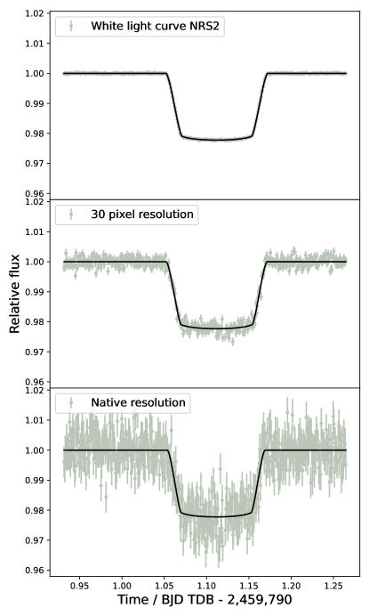
Figure 1: Fits to the white light curve as well as example fits, centred on $4.7$µm, to spectroscopic light curves at 30 pixel and native resolution. Shown are the corrected fluxes after the systematics model has been removed.

In stage 1 we largely utilise the JWST pipeline’s default processing steps. However, we skip the dark-current step owing to the present quality of available reference files. Additionally, after the jump-detection step is run, we “destripe” the data at the group level. Destriping involves subtracting the column-by-column median background value from each column’s pixels. This aims to reduce the 1/f noise at timescales longer than the column read time, or $440$µs, and is more effective when corrected for at the group-level (The JWST Transiting Exoplanet Community Early Release Science Team et al., 2023; Rustamkulov et al., 2023). These median values are computed with pixels having been flagged for poor data quality removed; and in particular, flagged pixels are made maximally consistent across groups within an integration. This flagging procedure ensures the same set of pixels are masked within a given pixel’s ramp, and we find this improves ramp continuity in the presence of transient outliers such as cosmic ray hits. After destriping, the default ramp-fitting step is run and rate-images are output from stage 1.

In stage 2 we utilise custom routines to clean the rate-images and extract a time series of stellar spectra. Outlier cleaning is performed by finding deviations from an estimated spatial profile, as is common in optimal extraction (Horne, 1986). However, the curved spectral trace means the spatial profile must be created piecewise from windowed row-wise polynomial fits, as has been similarly utilised by Zhang et al. (2021). We find a window size of 100 pixels, a polynomial order of 4, and an outlier threshold set at 4 standard deviations are sufficient to clean the curved spectral trace. Next, the background is subtracted column-by-column and the outlier cleaning is repeated once more. Stellar spectra are extracted using a box aperture centred on the spectral trace and with a width of 6 times the measured standard deviation of the point spread function. The resulting stellar spectra are comprised of between ${\sim}90,000$ and ${\sim}20,000$ electrons per column, decreasing from the short- to long-wavelength side of the NRS2 detector.

2.1 Transmission spectrum

From the stellar spectra, we generate a transmission spectrum at the highest resolution possible, to maximise our chances of detecting the fine-structure of the CO absorption band. To achieve this, we make spectroscopic light curves at the native resolution of NIRSpec’s G395H mode; these bins are just 2 pixels wide. For comparison, we also fit spectroscopic light curves with bins 30 pixels wide, as well as fit the entire NRS2 white light curve (see Figure 1). The light curves and transmission spectrum presented in Alderson et al. (2023) consisted of bins 10 pixels wide.

The data quality is such that systematics are barely visible in the raw light curves, with the exception of a small exponential ramp over the first ${\sim}10$ integrations, and a mirror tilt event at integration 269, as seen by Alderson et al. (2023). The exponential ramp is removed by discarding the first 15 integrations to ensure the full ramp effect does not impact the measured stellar baseline. The tilt event is accounted for by normalising the pre- and post-tilt flux by the pre- and post-transit median flux, respectively. We also discard three integrations immediately surrounding the tilt event. Any remaining systematics are modelled by linear regression of the measured relative positions of the spectral trace. These positions are found by cross-correlation in the dispersion direction using the median stellar spectra, and in the cross-dispersion direction using the median point spread function.

The total light curve model, $f(t)$, is described by

$$f(t)=T(t,\mathbf{\theta})+\sum_{j\in W}f_{0,j}+S_{j}(x_{j},y_{j}),$$ (1)

where

$$S_{j}(x_{j},y_{j})=p_{1,j}x_{j}+p_{2,j}y_{j}.$$ (2)

Here, $T$ is the physical transit model as a function of time, $t$, and transit parameter vector, $\mathbf{\theta}$. $f_{0}$ is an offset to the baseline flux. $S_{j}$ is the systematics model as a linear function of the spectral trace positions, $x_{j}$ and $y_{j}$. We elect to fit the non-physical model components piecewise, either side of the tilt event, where each window of data is denoted by the subscript $j$ from the set $W=\{\rm{pre{\text-}tilt},\rm{post{\text-}tilt}\}$. The $x_{j}$ and $y_{j}$ traces can be seen in Alderson et al. (2023, extended data figures 1 and 2), and for computational efficiency the values are standardised by subtracting their means and dividing by their standard deviations, independently for each $j$. For $T$ we use a Batman transit model (Kreidberg, 2015) with a fixed non-linear 4-parameter limb-darkening law computed using ExoTiC-LD (Grant & Wakeford, 2022) for each spectral bin using the 3D Stagger-grid of stellar models (Magic et al., 2015).

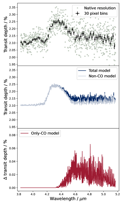
Figure 2: Top panel: observed transmission spectra at native resolution (green) and at 30 pixel resolution (black). Middle panel: model transmission spectrum fit to the data (dark blue) and the same model but with CO removed (grey). Bottom panel: model contribution from CO only (red).

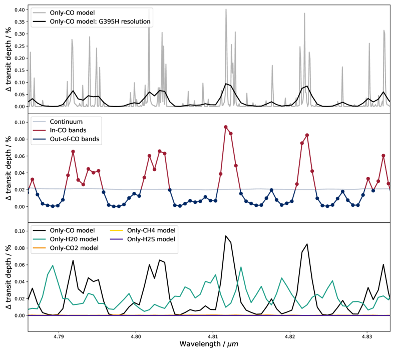
Figure 3: Top panel: example wavelength sector showing the model contribution from CO only. The model is shown at simulated resolution (grey, sampled every Ångstrom) and after being convolved with the observed point spread function and rebinned onto the detector’s wavelength grid (black). Middle panel: visualisation of our method for detecting CO sub-band structure. Red and blue portions indicate wavelengths that are in-band or out-of-band, respectively. Note these wavelength selections are refined in Figure 4. Bottom panel: model contributions per molecule, where H₂O is the only significant molecular absorber in this wavelength sector other than CO.

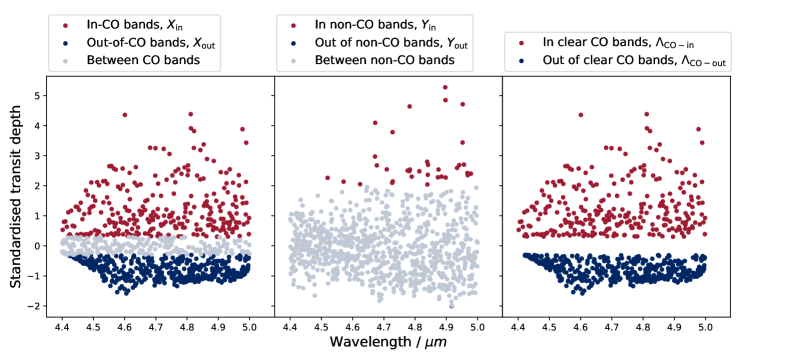
Figure 4: Graphical representation of the logic behind our in-band (red) and out-of-band (dark blue) definitions. The panels show the cuts in the models for the only-CO model (left-hand panel), the non-CO model (middle panel), and the resulting clear CO sub-bands model (right-hand panel).

We perform fitting of our light curve model with a least-squares optimiser (Virtanen et al., 2020), using the Levenberg-Marquadt algorithm (Moré, 1978), co-fitting the parameters $\mathbf{\theta}$, $f_{0,j}$, $p_{1,j}$, and $p_{2,j}$ simultaneously. We initially fit the white light curve to find the best-fit values for the center of transit time, $t_{0}=2459791.112128\pm 0.000021\,\mathrm{BJD}_{\mathrm{TDB}}$, semi-major axis, $a=11.395\pm 0.028\,\mathrm{R_{*}}$, and inclination $i=87.759\pm 0.028^{\circ}$. These values are then fixed in the spectroscopic light curve fits that follow. For each spectroscopic light curve fit, the standard deviation of the residuals is used to inflate the original uncertainties on the fluxes, and then the fits are repeated. The uncertainties in the resulting transit depths are computed from the square root of the inverse Hessian matrix. We validate this fast approximation by using a Markov chain Monte Carlo algorithm (Foreman-Mackey et al., 2013), with uniform priors, to sample the posterior distributions of several transit depths, and we find that the results are equivalent. These checks span the entire wavelength range of NRS2, with the inferred transit depths being on average 0.03 standard deviations discrepant and the corresponding uncertainties 1.7% different.

In Figure 1 we show fits to the white light curve, as well as example fits, centred on $4.7$µm, to spectroscopic light curves at 30 pixel and native resolution. In each panel, we show the corrected flux values with the systematics model removed. The systematics model accounts for on average $1.3\%$ of the residual variance, although close inspection of the light curves indicates a small amount of correlated noise remains. Tests varying the width of the spectral bins reveal the variance in the light curves becomes closer to the expected photon noise for narrower bins. This is indicative of the remaining noise being spatially correlated on the detector, most likely due to a small amount of leftover uncleaned 1/f noise. There is also likely some minor time-correlated noise, most clearly seen at the 30 pixel resolution, however we were unable to identify the origin of this noise. The mean residual standard deviations are 163 ppm, 1260 ppm, and 4644 ppm for the white light, 30 pixel, and native resolution light curve fits, respectively. At native resolution this precision corresponds to 1.1x photon noise. In the top panel of Figure 2 we show the transmission spectrum.

3 Theoretical models

To investigate the presence of CO in the transmission spectrum of WASP-39b, we fit the observations to a grid of PHOENIX atmosphere models (Hauschildt et al., 1999; Barman et al., 2001; Lothringer & Barman, 2020). This was the same grid used in the initial investigation of WASP-39b’s G395H spectrum in Alderson et al. (2023). The grid is sampled every Ångstrom and explores the irradiation temperature (i.e., absorbed heat from the star, $T_{\rm{irr}}$ = 1020, 1120, and 1220 K, respectively), internal temperature ($T_{\rm{int}}$ = 200 and 400 K), metallicity (0.1x, 1x, 10x, 50x, and 100x solar (Asplund et al., 2009)), C/O ratio (0.3, 0.54 (solar), 0.7, and 1.0), the presence of aerosols (a cloud deck at 0.3, 1, 3, and 10 mbar or a Rayleigh-scattering haze at 10x the H₂ scattering cross-section). We also included models with rainout chemistry (i.e., abundances of refractory elements are depleted in the layers above which they condense) compared to pure chemical equilibrium. Disequilibrium abundances of SO₂ from photochemistry (Tsai et al., 2022) were not included in these models. Species in the opacity calculation include CH, CH₄, CN, CO, CO₂, C₂, C₂H₂, C₂H₄, C₂H₆, CaH, CrH, FeH, HCN, HCl, HF, HI, HDO, HO₂, H₂, H₂S, H₂O, H₂O₂, H3⁺, MgH, NH, NH₃, NO, N₂, N₂O, OH, O₂, O₃, PH₃, SF₆, SiH, SiO, SiO₂, TiH, TiO, VO and atoms up to U. Of relevance for this work, we use the high-temperature CO linelist from Goorvitch (1994) that was used for the PHOENIX grid in Alderson et al. (2023), but we also test against the newer Li et al. (2015) list.

Our best-fit model at low-resolution, which we take to be our fiducial model, has $f$=0.351, $T_{\rm{int}}$ = 200 K, 10x solar metallicity, C/O = 0.3, a cloud deck at 0.3 mbar, no hazes, and rainout chemistry. These results are mostly consistent with those found using the median reduced G395H spectrum from 11 different analyses in Alderson et al. (2023), except for the internal temperature (200 versus 400 K) and the preference for rainout chemistry, both of which have relatively minor effects in the wavelength region probed by these G395H observations. We attribute this non-statistically-significant difference to the minor differences between data reductions.

We show the best-fit model compared to 30-pixel wide bins of the observations in the middle panel of Figure 2. Absorption from SO₂ at 4.0 µm and CO₂ at 4.3 µm are seen in the data, as previously described in The JWST Transiting Exoplanet Community Early Release Science Team et al. (2023); Alderson et al. (2023); Rustamkulov et al. (2023); Tsai et al. (2022). The middle panel also shows the model with and without the CO opacity. The difference of these two models is plotted in the bottom panel, indicating the contribution of CO to the best-fit transit spectrum. At the low effective resolution of 30 pixel bins, the presence of CO in the G395H spectrum is not apparent and its detection was not statistically justified due to blending with non-CO opacities like H₂O, CO₂ and the cloud opacity (Alderson et al., 2023).

4 Defining CO sub-bands

In order to detect the high-resolution features of CO, we define a set of wavelengths that are theorized to either display CO absorption (hereafter in-band) or not to display CO absorption (hereafter out-of-band). The aim is to compare the transit depths from each set, and thereby probe CO’s fundamental band structure. This method is displayed graphically in Figure 3. This plot shows how at the resolution of the G395 mode we are able to probe small clusters of CO lines, which together we refer to as sub-bands.

We set out to define these sub-bands such that they represent a good contrast between the in- versus out-of-band transit depth and, furthermore, are not biased towards finding other potential species’ high-resolution signals included in the atmospheric models. As we are concerned only with the high-resolution structure, we consider these sub-bands relative to the continuum level. We also restrict our analysis to the wavelength interval $4.4$µm $<\lambda<5.0$µm as this is the region that optimises the balance between the observed signal-to-noise and the amplitude of the model’s high-resolution CO structure. In this region the resolving power of the G395 mode ranges from $R\,{\sim}3040$ to ${\sim}3516$ with increasing wavelength.

Now, with the models for only-CO and non-CO in hand from Section 3, we layout a method for defining clear CO sub-bands. For each model, we remove the continuum with a Savitzky-Golay filter (Savitzky & Golay, 1964) and then standardise the mean and standard deviation of the model transit depths. To define the clear in-band wavelengths, $\Lambda_{\rm{CO{\text-}in}}$, we select the only-CO model transit depths above a set threshold, but only where these wavelengths do not show appreciable signals in the non-CO model. To define the clear out-of-band wavelengths, $\Lambda_{\rm{CO{\text-}out}}$, we use the same logic, but for only-CO model points below a set threshold. In this way, the sub-bands will probe the highest contrast regions of the CO signal, without inadvertently confusing the CO signal with other species. In terms of logical operators we can write

$$\Lambda_{\rm{CO{\text-}in}} =X_{\rm{in}}\,\rm{\textbf{\scalebox{0.9}{AND}}}\,(\,\rm{\textbf{\scalebox{0.9}{NOT}}}\,(Y_{\rm{in}}\,\rm{\textbf{\scalebox{0.9}{OR}}}\,Y_{\rm{out}})),$$ (3)

$$\Lambda_{\rm{CO{\text-}out}} =X_{\rm{out}}\,\rm{\textbf{\scalebox{0.9}{AND}}}\,(\,\rm{\textbf{\scalebox{0.9}{NOT}}}\,(Y_{\rm{in}}\,\rm{\textbf{\scalebox{0.9}{OR}}}\,Y_{\rm{out}})),$$ (4)

where $X_{\rm{in}}$ and $X_{\rm{out}}$ are wavelengths with only-CO model transit depths above and below set thresholds, and $Y_{\rm{in}}$ and $Y_{\rm{out}}$ are wavelengths with non-CO model transit depths above and below set thresholds, respectively.

As a graphical description, we display the selected wavelengths in Figure 4. Here, the clear in- and out-of-band wavelengths are shown in the right-hand panel. We set the threshold values to $\pm 0.3$ for $X$ and to $\pm 2.0$ for $Y$. The motivation for these threshold values is to balance the contrast of transit depth between in-band and out-of-band versus the number of bands included in the samples, and thus the statistical power of any detection test. These thresholds result in 259 clear bands, of which 111 are in-band and 148 are out-of-band. The distribution of the number of contiguous pixels in-band has a mean of 3.0 pixels and a standard deviation of 1.1 pixels. The distribution for out-of-band has a mean of 3.8 pixels and a standard deviation of 1.7 pixels.

5 Detecting CO sub-bands

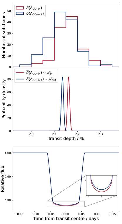
Figure 5: Top panel: samples showing the number of sub-bands as a function of transit depth, $\delta$, for in- and out-of-band CO. Middle panel: sampling distributions of the mean transit depths, $\overline{\delta}$, for in- and out-of-band CO. These sampling distributions are modelled as Gaussians with means and standard deviations inferred from the measured samples shown in the top panel. Bottom panel: light curve models visualising the measured difference in transit depth for in- and out-of-band CO.

Using our definition of CO sub-bands, we categorize the transit depths from the observed native-resolution transmission spectrum as either in-band or out-of-band. This process generates two samples of transit depths, one for each of the theorized underlying populations of transit depth for in-band and out-of-band. As in Section 4, we remove the continuum from the observed transit depths to probe only the high-resolution CO features. We display these two samples in the top panel of Figure 5. The CO in-band sample, $\delta(\Lambda_{\rm{CO{\text-}in}})$, has a mean, $\mu_{\rm{in}}=21616$ ppm, and standard deviation, $\sigma_{\rm{in}}=501$ ppm. The CO out-of-band sample, $\delta(\Lambda_{\rm{CO{\text-}out}})$, has a mean, $\mu_{\rm{out}}=21352$ ppm, and standard deviation, $\sigma_{\rm{out}}=576$ ppm.

To test statistically if the in-band sample displays greater CO absorption than the out-of-band sample, we conduct a hypothesis test. We run a two-sample T-test, specifically a one-tailed Welch’s t-test (Welch, 1947), with the following hypothesis:

$$\mathcal{H}_{0} :\mu_{\rm{in}}=\mu_{\rm{out}},$$ (5)

$$\mathcal{H}_{1} :\mu_{\rm{in}}>\mu_{\rm{out}},$$ (6)

where $\mathcal{H}_{0}$ and $\mathcal{H}_{1}$ are the null and alternate hypotheses, respectively. Running this test on our samples, we find a statistically significant result. The in-band samples have a greater mean transit depth than the out-of-band samples, with $t=3.90$ and $p=0.00006$, and hence we detect high-resolution CO band structure with assurance.

As a visual representation, we plot the sampling distributions of the mean transit depths in the middle panel of Figure 5. The sampling distributions are normally distributed such that

$$\overline{\delta}(\Lambda_{\rm{CO{\text-}in}}) \sim\mathcal{N}\Big{(}\mu_{\rm{in}},\frac{\sigma^{2}_{\rm{in}}}{n_{\rm{in}}}\Big{)},$$ (7)

$$\overline{\delta}(\Lambda_{\rm{CO{\text-}out}}) \sim\mathcal{N}\Big{(}\mu_{\rm{out}},\frac{\sigma^{2}_{\rm{out}}}{n_{\rm{out}}}\Big{)},$$ (8)

where the standard errors are $\sigma_{\rm{in}}/n_{\rm{in}}^{1/2}=48$ ppm and $\sigma_{\rm{out}}/n_{\rm{out}}^{1/2}=48$ ppm, and the sample sizes are given by $n_{\rm{in}}$ and $n_{\rm{out}}$. The difference between the transit depth means is $264\pm 68$ ppm. This difference, in terms of the resulting light curve models, is displayed in the bottom panel of Figure 5.

Further to this result, we conduct sensitivity tests for the $X$ and $Y$ thresholds set in Section 4. We find that our results are not sensitive to the $Y$ threshold, but when varying the $X$ threshold we observe a change in the detected transit depth difference between in-band and out-of-band samples. As the $X$ threshold increases the transit depth difference increases, but with increasing uncertainty owing to the reduced statistical power. For example, if the $X$ threshold values are increased to $\pm 0.4$, the difference between the transit depth means becomes $301\pm 81$ ppm. Intuitively this effect can be understood as the larger thresholds narrowing in on the peaks of the CO sub-bands, where the contrast in transit depth is greater but fewer data points lie.

6 Discussion

The technique presented works particularly well with JWST’s NIRSpec G395H mode, owing to its comparatively high spectral resolution. Given this resolution, it was vital in our analysis to account for the Doppler transformations of both the barycentric velocity of the WASP-39 system, $\gamma_{*}=-58.4421\,\rm{\,km\,s^{-1}}$ (Mancini et al., 2018), and of JWST’s barycentric velocity at the time of observation, $\gamma_{\rm{\scalebox{0.6}{JWST}}}=-28.88807\,\rm{\,km\,s^{-1}}$. In fact, the robustness of our detection is further backed up by trialing spurious Doppler transformations. We find that shifting our models by velocities equivalent to just one resolution element ($\pm 88\,\rm{\,km\,s^{-1}}$ at 4.5 µm) in either direction leads to non-detections, with $p=0.42$ and $0.17$. This further highlights the fidelity and soundness of our detection, whilst also underscoring the need for models applied to the highest resolution JWST modes to be appropriately Doppler shifted when searching for narrow molecular features.

Our technique offers an independent test for the presence of molecular features in the atmospheres of exoplanets for well characterised molecules with precise line lists. Differences in the measured excess transit depth of only 4 ppm were found using the different CO line lists of Goorvitch (1994) and Li et al. (2015), though such differences may be greater in the overtone bands where the two lists disagree more than in the fundamental band. The technique may be applied to other molecules with rotational sub-band structures distinctly separated at $R\,{\sim}3000$, for example CH₄, NH₃, or HCN between 2.5 and 3.5 µm, but the development and use of accurate and complete line lists for other species is necessary. The structure may be more difficult to measure for molecules such as H₂O that are more easily distinguished by their broadband structure due to the ro-vibrational lines being more tightly clustered.

Aside from the technique outlined in this work, cross-correlation methods, often used with high-resolution ground-based data, may also be applied to the highest resolution JWST modes. Certain cross-correlation formalisms (e.g., Brogi & Line, 2019; Gibson et al., 2020) enable the construction of a likelihood function which can also be used for the detection and retrieval of molecules and their abundances, and a future methodology comparison with traditional low-resolution methods may be fruitful.

7 Summary and conclusions

We have detected absorption structure in CO’s fundamental band using JWST’s NIRSpec G395H mode. To make this detection we employed a new technique in which we categorized wavelength bins as either in-band or out-of-band, and then compared the transit depths of the resulting samples. We found the mean transit depth of CO sub-bands to be $264\pm 68$ ppm larger than the transit depth between CO sub-bands. This value is in agreement with the prediction from the PHOENIX model spectrum of $217$ ppm, when using the same sub-bands.

While CO₂’s opacity is much stronger per molecule in the G395H wavelength regime and was therefore more easily detected in Alderson et al. (2023), CO is actually by-far the dominant carbon-bearing molecule throughout WASP-39b’s atmosphere with a 1 mbar volume mixing ratio in the best-fit model of 2,326 ppm compared to 7 ppm of CO₂. This fact remains true for all giant planets in chemical equilibrium with plausible heavy-element enrichments (e.g., $M/H\leq 100$x solar). Thus the detection of CO, in addition to CO₂, enables a more robust and complete understanding of a planet’s chemical inventory, especially with respect to the measurement of the C/O ratio. Without such a measurement, any inference of the bulk carbon abundance or C/O ratio from CO₂ alone would rely on assumptions of chemical equilibrium. We can therefore not only be more confident in the detection of CO with JWST/NIRSpec/PRISM (Rustamkulov et al., 2023), but also in the conclusions from the other JWST spectra that WASP-39b has a sub-solar to solar C/O ratio and likely formed interior to the CO₂ ice line (Alderson et al., 2023; Ahrer et al., 2023; Feinstein et al., 2023).

References

- Ahrer et al. (2023) Ahrer, E.-M., Stevenson, K. B., Mansfield, M., et al. 2023, Nature, arXiv:2211.10489. https://arxiv.org/abs/2211.10489
- Alderson et al. (2022) Alderson, L., Grant, D., & Wakeford, H. 2022, Exo-TiC/ExoTiC-JEDI: v0.1-beta-release, v0.1, Zenodo, doi: 10.5281/zenodo.7185855
- Alderson et al. (2023) Alderson, L., Wakeford, H. R., Alam, M. K., et al. 2023, Nature, 1. https://arxiv.org/abs/2211.10488
- Asplund et al. (2009) Asplund, M., Grevesse, N., Sauval, A. J., & Scott, P. 2009, ARA&A, 47, 481, doi: 10.1146/annurev.astro.46.060407.145222
- Astropy Collaboration et al. (2013) Astropy Collaboration, Robitaille, T. P., Tollerud, E. J., et al. 2013, A&A, 558, A33, doi: 10.1051/0004-6361/201322068
- Astropy Collaboration et al. (2018) Astropy Collaboration, Price-Whelan, A. M., Sipőcz, B. M., et al. 2018, AJ, 156, 123, doi: 10.3847/1538-3881/aabc4f
- Barman et al. (2001) Barman, T. S., Hauschildt, P. H., & Allard, F. 2001, ApJ, 556, 885, doi: 10.1086/321610
- Barman et al. (2015) Barman, T. S., Konopacky, Q. M., Macintosh, B., & Marois, C. 2015, ApJ, 804, 61, doi: 10.1088/0004-637X/804/1/61
- Bean et al. (2018) Bean, J. L., Stevenson, K. B., Batalha, N. M., et al. 2018, PASP, 130, 114402, doi: 10.1088/1538-3873/aadbf3
- Birkmann et al. (2022) Birkmann, S., Ferruit, P., Giardino, G., et al. 2022, Astronomy & Astrophysics, 661, A83
- Brogi et al. (2014) Brogi, M., de Kok, R. J., Birkby, J. L., Schwarz, H., & Snellen, I. A. G. 2014, A&A, 565, A124, doi: 10.1051/0004-6361/201423537
- Brogi & Line (2019) Brogi, M., & Line, M. R. 2019, The Astronomical Journal, 157, 114
- Bushouse et al. (2022) Bushouse, H., Eisenhamer, J., Dencheva, N., et al. 2022, JWST Calibration Pipeline, 1.6.2, Zenodo, doi: 10.5281/zenodo.7041998
- Cushing et al. (2005) Cushing, M. C., Rayner, J. T., & Vacca, W. D. 2005, ApJ, 623, 1115, doi: 10.1086/428040
- de Kok et al. (2013) de Kok, R. J., Brogi, M., Snellen, I. A. G., et al. 2013, A&A, 554, A82, doi: 10.1051/0004-6361/201321381
- Encrenaz et al. (2004) Encrenaz, T., Lellouch, E., Drossart, P., et al. 2004, Astronomy & Astrophysics, 413, L5
- Faedi et al. (2011) Faedi, F., Barros, S. C. C., Anderson, D. R., et al. 2011, A&A, 531, A40, doi: 10.1051/0004-6361/201116671
- Feinstein et al. (2023) Feinstein, A. D., Radica, M., Welbanks, L., et al. 2023, Nature, 1. https://arxiv.org/abs/2211.10493
- Foreman-Mackey et al. (2013) Foreman-Mackey, D., Hogg, D. W., Lang, D., & Goodman, J. 2013, Publications of the Astronomical Society of the Pacific, 125, 306
- Giacobbe et al. (2021) Giacobbe, P., Brogi, M., Gandhi, S., et al. 2021, Nature, 592, 205, doi: 10.1038/s41586-021-03381-x
- Gibson et al. (2020) Gibson, N. P., Merritt, S., Nugroho, S. K., et al. 2020, Monthly Notices of the Royal Astronomical Society, 493, 2215
- Goorvitch (1994) Goorvitch, D. 1994, ApJS, 95, 535, doi: 10.1086/192110
- Grant & Wakeford (2022) Grant, D., & Wakeford, H. R. 2022, Exo-TiC/ExoTiC-LD: ExoTiC-LD v3.0.0, v3.0.0, Zenodo, doi: 10.5281/zenodo.7437681
- Harris et al. (2020) Harris, C. R., Millman, K. J., van der Walt, S. J., et al. 2020, Nature, 585, 357, doi: 10.1038/s41586-020-2649-2
- Hauschildt et al. (1999) Hauschildt, P. H., Allard, F., & Baron, E. 1999, ApJ, 512, 377, doi: 10.1086/306745
- Heng & Lyons (2016) Heng, K., & Lyons, J. R. 2016, The Astrophysical Journal, 817, 149
- Hoeijmakers et al. (2018) Hoeijmakers, H. J., Schwarz, H., Snellen, I. A. G., et al. 2018, A&A, 617, A144, doi: 10.1051/0004-6361/201832902
- Horne (1986) Horne, K. 1986, Publications of the Astronomical Society of the Pacific, 98, 609
- Hoyer & Hamman (2017) Hoyer, S., & Hamman, J. 2017, Journal of Open Research Software, 5, doi: 10.5334/jors.148
- Hoyer et al. (2022) Hoyer, S., Roos, M., Joseph, H., et al. 2022, xarray, v2022.03.0, Zenodo, doi: 10.5281/zenodo.6323468
- Hunter (2007) Hunter, J. D. 2007, Computing in Science & Engineering, 9, 90, doi: 10.1109/MCSE.2007.55
- Jakobsen et al. (2022) Jakobsen, P., Ferruit, P., de Oliveira, C. A., et al. 2022, Astronomy & Astrophysics, 661, A80
- Konopacky et al. (2013) Konopacky, Q. M., Barman, T. S., Macintosh, B. A., & Marois, C. 2013, Science, 339, 1398, doi: 10.1126/science.1232003
- Kreidberg (2015) Kreidberg, L. 2015, Publications of the Astronomical Society of the Pacific, 127, 1161
- Li et al. (2015) Li, G., Gordon, I. E., Rothman, L. S., et al. 2015, ApJS, 216, 15, doi: 10.1088/0067-0049/216/1/15
- Line et al. (2021) Line, M. R., Brogi, M., Bean, J. L., et al. 2021, Nature, 598, 580, doi: 10.1038/s41586-021-03912-6
- Lodders & Fegley (1998) Lodders, K., & Fegley, B. 1998, The planetary scientist’s companion / Katharina Lodders, Bruce Fegley.
- Lodders & Fegley (2002) —. 2002, Icarus, 155, 393, doi: 10.1006/icar.2001.6740
- Lothringer & Barman (2020) Lothringer, J. D., & Barman, T. S. 2020, AJ, 159, 289, doi: 10.3847/1538-3881/ab8d33
- Magic et al. (2015) Magic, Z., Chiavassa, A., Collet, R., & Asplund, M. 2015, Astronomy & Astrophysics, 573, A90
- Mancini et al. (2018) Mancini, L., Esposito, M., Covino, E., et al. 2018, Astronomy & Astrophysics, 613, A41
- Miles et al. (2022) Miles, B. E., Biller, B. A., Patapis, P., et al. 2022, arXiv e-prints, arXiv:2209.00620. https://arxiv.org/abs/2209.00620
- Moré (1978) Moré, J. J. 1978, in Numerical analysis (Springer), 105–116
- pandas development team (2022) pandas development team, T. 2022, pandas-dev/pandas: Pandas 1.4.3, v1.4.3, Zenodo, doi: 10.5281/zenodo.6702671
- Petit dit de la Roche et al. (2018) Petit dit de la Roche, D. J. M., Hoeijmakers, H. J., & Snellen, I. A. G. 2018, A&A, 616, A146, doi: 10.1051/0004-6361/201833384
- Price-Whelan et al. (2022) Price-Whelan, A. M., Lim, P. L., Earl, N., et al. 2022, The Astrophysical Journal, 935, 167
- Rustamkulov et al. (2023) Rustamkulov, Z., Sing, D. K., Mukherjee, S., et al. 2023, Nature, 1. https://arxiv.org/abs/2211.10487
- Savitzky & Golay (1964) Savitzky, A., & Golay, M. 1964, Analytical Chemistry, 36, 1627, doi: 10.1021/ac60214a047
- Schwarz et al. (2015) Schwarz, H., Brogi, M., De Kok, R., Birkby, J., & Snellen, I. 2015, Astronomy & Astrophysics, 576, A111
- Snellen et al. (2015) Snellen, I., de Kok, R., Birkby, J. L., et al. 2015, A&A, 576, A59, doi: 10.1051/0004-6361/201425018
- Snellen et al. (2010) Snellen, I. A. G., de Kok, R. J., de Mooij, E. J. W., & Albrecht, S. 2010, Nature, 465, 1049, doi: 10.1038/nature09111
- Stevenson et al. (2016) Stevenson, K. B., Lewis, N. K., Bean, J. L., et al. 2016, PASP, 128, 094401, doi: 10.1088/1538-3873/128/967/094401
- The JWST Transiting Exoplanet Community Early Release Science Team et al. (2023) The JWST Transiting Exoplanet Community Early Release Science Team, Ahrer, E.-M., Alderson, L., et al. 2023, Nature, arXiv:2208.11692. https://arxiv.org/abs/2208.11692
- Tsai et al. (2022) Tsai, S.-M., Lee, E. K. H., Powell, D., et al. 2022, accepted for publication in Nature, arXiv:2211.10490. https://arxiv.org/abs/2211.10490
- Virtanen et al. (2020) Virtanen, P., Gommers, R., Oliphant, T. E., et al. 2020, Nature Methods, 17, 261, doi: 10.1038/s41592-019-0686-2
- Welch (1947) Welch, B. L. 1947, Biometrika, 34, 28
- Zhang et al. (2021) Zhang, M., Knutson, H. A., Wang, L., et al. 2021, The Astronomical Journal, 161, 181