A descent method for nonsmooth multiobjective optimization problems on Riemannian manifolds

Abstract

In this paper, a descent method for nonsmooth multiobjective optimization problems on complete Riemannian manifolds is proposed. The objective functions are only assumed to be locally Lipschitz continuous instead of convexity used in existing methods. A necessary condition for Pareto optimality in Euclidean space is generalized to the Riemannian setting. At every iteration, an acceptable descent direction is obtained by constructing a convex hull of some Riemannian $\varepsilon$-subgradients. And then a Riemannian Armijo-type line search is executed to produce the next iterate. The convergence result is established in the sense that a point satisfying the necessary condition for Pareto optimality can be generated by the algorithm in a finite number of iterations. Finally, some preliminary numerical results are reported, which show that the proposed method is efficient.

1 Introduction

In the field of optimization, minimizing multiple objective functions at the same time is called multiobjective optimization. Usually, these objective functions are conflicting with each other, instead of having some common minimum points. For example, producers want to create higher value and make the cost as low as possible in production and manufacturing. Similar problems arise in many applications such as engineering design Engau , management science Uttarayan Bagchi ; M. Gravel , environmental analysis Leschine ; Fliege1 , etc. Due to its wide practical applications, multiobjective optimization has always been a hot topic, and a rich literature was produced; see the monographs Abraham ; Deb ; Sawaragi and the references therein.

In most cases, the solution of multiobjective optimization problem is not a single point but a set of all optimal compromises, namely, the Pareto set. In traditional multiobjective optimization, one of the most popular methods is the scalarization approach Geoffrion , whose idea is to convert a multiobjective problem to a single or a family of single objective optimization problems. However, in this method, the users need to select some necessary parameters because they are not known in advance, which may bring an additional cost. To overcome this shortcoming, there have other methods to solve such optimization problems, such as descent methods Fliege Steepest ; El ; Gebken B , Newton-type methods Fliege Newton ; Povalej Ž , proximal point methods H. Bonnel ; Bento6 and proximal bundle methods Makela1 , etc. These methods are almost all developed from a single objective optimization. In this paper, we are particularly interested in the case where the objective functions are not necessarily differentiable or convex. Recently, Gebken and Peitz Gebken B proposed a descent method for locally Lipschitz multiobjective optimization, in which an acceptable descent direction for all objectives is selected as the element which has the smallest norm in the negative convex hull of certain subgradients of the objective functions.

In recent years, many traditional single objective optimization theories and methods have been extended from Euclidean space to Riemannian manifolds; see, e.g., P. A. Absil ; Boumal ; Hosseini1 ; Huang W ; Hu ; Hoseini ; Sato ; Zhu X . Comparatively, for Riemannian multiobjective optimization, the relevant literature is very scarce, especially for nonsmooth cases. In Bento1 and Bento2 , a steepest descent method and an inexact version with Armijo rule for multiobjective optimization in the Riemannian context are presented, respectivley. Both methods require the objective functions to be continuously differentiable for partial convergence, and further assume that the objective vector function is quasi-convex and the manifold has nonnegative curvature for full convergence. In Bento3 , a proximal point method for nonsmooth multiobjective optimization on Hadamard manifold is developed. In Bento4 , a subgradient-type method for Riemannian nonsmooth multiobjective optimization is presented, which requires the objective vector function to be convex. In Eslami N , a trust region method for Riemannian smooth multiobjective optimization problems is proposed. As far as we know, numerical results are not reported in the existing literature for Riemannian nonsmooth multiobjective optimization.

Based on the above observations, the aim of this paper is to develop a practical implementable method for nonconvex nonsmooth multiobjective optimization problems on general Riemannian manifolds. More precisely, we propose a descent method for locally Lipschitz multiobjective optimization problems on complete Riemannian manifolds, which can be regarded as an extension of the work Gebken B in Euclidean space. To the best of our knowledge, our work is the first to consider the setting discussed here. The classical necessary condition of the Pareto optimal points for nonsmooth multiobjective optimization (see Makela2 ) is generalized to the Riemannian setting. The Riemannian $\varepsilon$-subdifferential is introduced by using the isometric vector transports which satisfy a locking condition Hosseini2 . And then show that there exists a common descent direction for each objective, which is just the element with the smallest norm in the set consisting of the negative convex hull of the Riemannian $\varepsilon$-subdifferentials of all objective functions. Of course, it is generally not easy to compute the $\varepsilon$-subdifferentials of a nonsmooth function especially when its domain is a manifold. In order to save computational effort, inspired by the strategy adopted in the traditional methods Mahdavi-Amiri ; Gebken B , we use the convex hull of a special set to approximate the convex hull of Riemannian $\varepsilon$-subdifferentials of all objective functions. For this set, at the beginning, it consists of a single $\varepsilon$-subgradient of each objective function, then some new $\varepsilon$-subgradients are systematically computed and added to enrich the set, until the element with the smallest norm in its convex hull is an acceptable direction for each objective function. Furthermore, a Riemannian Armijo-type line search is executed to produce the next iterate. The convergence result is established in the sense that an $(\varepsilon,\delta)$-critical point which is an approximation of the Pareto optimal point can be generated in a finite number of iterations. Finally, some preliminary numerical results are reported, which show that the proposed method is efficient.

This paper is organized as follows. In section 2, we recall some basic notations and definitions regarding Riemannian manifolds and locally Lipschitz function. In section 3, the necessary condition for Pareto optimality regarding locally Lipschitz multiobjective optimization problems is generalized to Riemannian manifolds, and the details of our method is presented. In section 4, we establish the convergence result of our method. In section 5, some preliminary numerical experiments are given.

2 Preliminaries

Throughout of the paper, we denote by cl$S$ and conv$S$ the closure and the convex hull of a set $S$, respectively. Letting $\mathcal{M}$ be a complete $d$-dimensional ($d\geq 1$) smooth manifold endowed with a Riemannian metric $\langle\cdot,\cdot\rangle_{x}$ on the tangent space $T_{x}\mathcal{M}$, we denote by $\|\cdot\|_{x}$ the norm which induced by Riemannian metric. We will often omit subscripts when they do not cause confusion and simply write $\langle\cdot,\cdot\rangle$ and $\|\cdot\|$ to $\langle\cdot,\cdot\rangle_{x}$ and $\|\cdot\|_{x}$, respectively. The Riemannian distance from $x$ to $y$ is denoted by dist($x$,$y$), where the points $x,y\in\mathcal{M}$. Denote $\mathbb{B}(x,\sigma)=\{y\in\mathcal{M}|\,\,{\rm dist}(x,y)<\sigma\}$, and the tangent bundle by $T\mathcal{M}$.

Firstly, we introduce the definition of locally Lipschitz functions on Riemannian manifolds; see, e.g., Hosseini1 .

Definition 1

Let $x\in\mathcal{M}$, $L>0$, and $\mathcal{N}\subset\mathcal{M}$ be a neighborhood of $x$. If $f:\mathcal{M}\rightarrow\mathbb{R}$ satisfies

$$|f(x)-f(y)|\leq L{\rm dist}(x,y),\,\,{\rm for}\,\,{\rm all}\,\,y\in\mathcal{N},$$

we say that $f$ is Lipschitz continuous near $x$ with the constant $L$. Furthermore, if for all $x\in\mathcal{M}$, $f$ is Lipschitz continuous near $x$, then we say that $f$ is a locally Lipschitz (continuous) function on $\mathcal{M}$.

Now we consider the Riemannian nonsmooth multiobjective optimization problem:

$$\min_{x\in\mathcal{M}}F(x):=\left(\begin{array}[]{ll}f_{1}(x)\\ \,\,\,\,\,\,\vdots\\ f_{m}(x)\end{array}\right),$$ (4)

where $F:\mathcal{M}\rightarrow\mathbb{R}^{m}$ is called objective vector function, and the components $f_{i}:\mathcal{M}\rightarrow\mathbb{R}$ for $i\in\{1,\cdots,m\}$ are called objective functions, which are assumed to be locally Lipschitz continuous on $\mathcal{M}$. Clearly, the concept of optimality for real-valued function no longer applies, since the objective function of problem (4) is vector valued. So we introduce the following so-called Pareto optimality (see (Ehrgott, , Ch. 2)), and our aim is to find (approximate) Pareto optimal points on manifolds.

Definition 2

Let $x\in\mathcal{M}$. If there is no $y\in\mathcal{M}$ such that

$$f_{i}(y)\leq f_{i}(x)\,\,\,\,\forall i\in\{1,\cdots,m\}\,\,{\rm and}\,\,f_{j}(y)<f_{j}(x)\,\,\,\,{\rm for\,\,some}\,\,j\in\{1,\cdots,m\},$$

then we say that $x$ is a Pareto optimal point for the problem (4). Pareto set is the set consisting of all Pareto optimal points.

For optimization problems posed on nonlinear manifolds, the concept of retraction can help us to develop a theory which is similar to line search methods in $\mathbb{R}^{n}$; see (P. A. Absil, , Def. 4.1.1).

Definition 3

A smooth mapping $R:T\mathcal{M}\rightarrow\mathcal{M}$ is called a retraction on a manifold $\mathcal{M}$ if it has the following properties:

(i) $R_{x}(0_{x})=x$, where $0_{x}$ denotes the zero element of $T_{x}\mathcal{M}$;

(ii) with the canonical identification $T_{0_{x}}T_{x}\mathcal{M}\simeq T_{x}\mathcal{M}$, $R_{x}$ satisfies

$${\rm D}R_{x}(0_{x})={\rm id}_{T_{x}\mathcal{M}},$$

where $R_{x}$ is the restriction of $R$ to $T_{x}\mathcal{M}$, and ${\rm id}_{T_{x}\mathcal{M}}$ denotes the identity mapping on $T_{x}\mathcal{M}$.

It is further assumed that there is a constant $\kappa$ such that

$${\rm dist}(R_{x}(\xi_{x}),x)\leq\kappa\|\xi_{x}\|$$ (5)

for all $x\in\mathcal{M}$ and $\xi_{x}\in T_{x}\mathcal{M}$. Intuitively, the inequality (5) implies that the distance between $x$ and $R_{x}(\xi_{x})$ is bounded when the vector $\xi_{x}$ is bounded. Furthermore, it can ensure that the point $R_{x}(\xi_{x})$ is in the neighborhood of $x$ when $\|\xi_{x}\|$ is small enough. This does not constitute any restriction in most cases of interest; see Hosseini1 . Denote $B_{R}(x,r)=\{R_{x}(\eta_{x})|\,\,\|\eta_{x}\|<r\}$, which is an open ball centered at $x$ with radius $r$ if the retraction $R$ is the exponential mapping; see Hosseini2 .

Since we will work in different tangent spaces, it is necessary to introduce the concept of vector transport (see (P. A. Absil, , Def. 8.1.1)). As its name implies, it serves to move vectors in different tangent spaces to the same tangent space. Particularly, parallel translation along geodesics is a vector transport.

Definition 4

A smooth mapping $\mathcal{T}:T\mathcal{M}\oplus T\mathcal{M}\rightarrow T\mathcal{M}:(\eta_{x},\xi_{x})\mapsto\mathcal{T}_{\eta_{x}}(\xi_{x})$ is said to be a vector transport associated to a retraction $R$ if for all $(\eta_{x},\xi_{x})$, the following conditions hold:

(i) $\mathcal{T}_{\eta_{x}}:T_{x}\mathcal{M}\rightarrow T_{R_{x}(\eta_{x})}\mathcal{M}$ is a linear map;

(ii) $\mathcal{T}_{0_{x}}(\xi_{x})=\xi_{x}$ for all $\xi_{x}\in T_{x}\mathcal{M}$.

Briefly, if $\xi_{x}\in T_{x}\mathcal{M}$ and $R(\eta_{x})=y$, then $\mathcal{T}_{\eta_{x}}$ transports vector $\xi_{x}$ from the tangent space of $\mathcal{M}$ at $x$ to the tangent space at $y$. In order to obtain convergence results, the following conditions are also required.

$\bullet$

The vector transport $\mathcal{T}$ preserves inner products, i.e.,

$$\langle\mathcal{T}_{\eta_{x}}(\xi_{x}),\mathcal{T}_{\eta_{x}}(\zeta_{x})\rangle=\langle\xi_{x},\zeta_{x}\rangle.$$ (6)

$\bullet$

The following locking condition is satisfied for $\mathcal{T}$, i.e.,

$$\mathcal{T}_{\xi_{x}}(\xi_{x})=\beta_{\xi_{x}}\mathcal{T}_{R_{\xi_{x}}}(\xi_{x}),\quad\beta_{\xi_{x}}=\frac{\|\xi_{x}\|}{\|\mathcal{T}_{R_{\xi_{x}}}(\xi_{x})\|},$$ (7)

where

$$\mathcal{T}_{R_{\eta_{x}}}(\xi_{x})={\rm D}R_{x}(\eta_{x})[\xi_{x}]=\frac{\rm d}{{\rm d}t}R_{x}(\eta_{x}+t\xi_{x})|_{t=0}.$$

The above conditions are satisfied with $\beta_{\xi_{x}}=1$ if the retraction and vector transport are selected as the exponential map and parallel transport, respectively; see Huang W for more details. For simplicity, the following intuitive notations are used:

$$\mathcal{T}_{x\rightarrow y}(\xi_{x}):=\mathcal{T}_{\eta_{x}}(\xi_{x}),\,\,{\rm and}\,\,\mathcal{T}_{x\leftarrow y}(\xi_{x}):=(\mathcal{T}_{\eta_{x}})^{-1}(\xi_{y})\,\,{\rm whenever}\,\,y=R_{x}(\eta_{x}).$$

In addition, it is necessary to introduce the notion of injectivity radius for $R_{x}$, since we need to transport subgradients from tangent spaces at some points lying in the neighborhood of $x\in\mathcal{M}$ to the tangent space at $x$; see Hosseini2 .

Definition 5

Let

$$\iota(x):={\rm sup}\{\varepsilon>0|\,\,R_{x}:B(0_{x},\varepsilon)\rightarrow B_{R}(x,\varepsilon){\rm\,\,is\,\,injective}\},$$

where $B(0_{x},\varepsilon)=\{\xi_{x}|\,\,\|\xi_{x}\|<\varepsilon\}\subset T_{x}\mathcal{M}$. Furthermore, for this retraction $R$, the injectivity radius of $\mathcal{M}$ is defined as

$$\iota(\mathcal{M}):=\inf_{x\in\mathcal{M}}\iota(x).$$

Remark 1

(i) As in usual we assume that $\iota(\mathcal{M})>0$, and that an explicit positive lower bound of $\iota(\mathcal{M})$ is available, which will be used as an input of the algorithm. In fact, when $\mathcal{M}$ is compact, we at least know that $\iota(\mathcal{M})>0$. (ii) Clearly, $\mathcal{T}_{x\leftarrow y}(\xi_{x})$ is well defined for all $y\in B_{R}(x,\iota(x))$, especially, for all $y\in B_{R}(x,\iota(\mathcal{M}))$. In what follows, it will always be ensured that $\mathcal{T}_{x\leftarrow y}(\xi_{x})$ is well defined when we use it.

We close this section by recalling the notion of Riemannian subdifferential, which is an extension of the classical Clarke subdifferential; see Hosseini2 . If $X$ is a Hilbert space, and $\phi$ is a locally Lipschitz function defined from $X$ to $\mathbb{R}$, the Clarke generalized directional derivative of $\phi$ at $x$ in direction $v$ is defined as

$$\phi^{\circ}(x;v)=\limsup_{y\rightarrow x,\,\,t\downarrow 0}\frac{\phi(y+tv)-\phi(y)}{t},$$

and the Clarke subdifferential of $\phi$ at $x$ is then given by

$$\partial\phi(x):=\{\xi\in X\mid\langle\xi,v\rangle\leq\phi^{\circ}(x;v)\,\,{\rm for}\,\,{\rm all}\,\,v\in X\}.$$

Definition 6

Let $f:\mathcal{M}\rightarrow\mathbb{R}$ be a locally Lipschitz function and for $x\in\mathcal{M}$, denote $\hat{f}_{x}=f\circ R_{x}$. The Riemannian directional derivative of $f$ at $x$ in direction $p\in T_{x}\mathcal{M}$ is defined as

$$f^{\circ}(x;p)=\hat{f}^{\circ}_{x}(0_{x},p),$$

where $\hat{f}^{\circ}_{x}(0_{x},p)$ is the Clarke generalized directional derivative of $\hat{f}_{x}:T_{x}\mathcal{M}\rightarrow\mathbb{R}$ at $0_{x}$ in direction $p\in T_{x}\mathcal{M}$. Then the Riemannian subdifferential of $f$ at $x$ is defined as

$$\partial f(x)=\partial\hat{f}_{x}(0_{x}).$$

The following lemma shows some important properties of the Riemannian subdifferential, which are similar to those of the Clarke subdifferential in Hilbert space; see (Hosseini2, , Thm. 2.2).

Lemma 1

Let $f:\mathcal{M}\rightarrow\mathbb{R}$ be a locally Lipschitz function, then the set $\partial f(x)$ is a nonempty, compact and convex subset of $T_{x}\mathcal{M}$, and $\|\xi\|\leq L$ for all $\xi\in\partial f(x)$, where $L$ is the Lipschitz constant near $x$.

The Riemannian $\varepsilon$-subdifferential and $\varepsilon$-subgradient of $f$ can be also defined; see Hosseini2 .

Definition 7

Let $\varepsilon\in\left(0,\frac{1}{2}\iota(x)\right)$, then the Riemannian $\varepsilon$-subdifferential of a locally Lipschitz function $f$ on a Riemannian manifold $\mathcal{M}$ at $x$ is defined as

$$\partial_{\varepsilon}f(x):={\rm cl\,conv}\{\beta_{\eta}^{-1}\mathcal{T}_{x\leftarrow y}(\partial f(y)):\ y\in{\rm cl}B_{R}(x,\varepsilon)\,\,{\rm and}\,\,\eta=R_{x}^{-1}(y)\},$$

where $\beta_{\eta}=\frac{\|\eta\|}{\|\mathcal{T}_{R_{\eta}}(\eta)\|}$. Every element of $\partial_{\varepsilon}f(x)$ is called a (Riemannian) $\varepsilon$-subgradient.

Lemma 2

The set $\partial_{\varepsilon}f(x)$ is a nonempty, compact and convex subset of $T_{x}\mathcal{M}$.

Proof

From (Hosseini2, , Thm. 2.15) we know that the set $\partial_{\varepsilon}f(x)$ is bounded. This together with Lemma 1 and Definition 7 shows the claim. ∎

3 A descent method for Riemannian nonsmooth multiobjective optimization

In this section, we present the details of our algorithm, which contains two procedures that help us to find a descent direction. We first introduce the definition of global weak Pareto optimal and local weak Pareto optimal for problem (4) as follows; see (Ehrgott, , Ch. 2).

Definition 8

Let $x\in\mathcal{M}$. If there is no $y\in\mathcal{M}$ such that $f_{i}(y)<f_{i}(x)$ for all $i=1,\cdots,m$, then we say that $x$ is a weak Pareto optimal of problem (4). If there exists some $\sigma>0$ such that $x$ is a (weak) Pareto optimal on $\mathbb{B}(x,\sigma)\cap\mathcal{M}$, then we say that $x$ is a local (weak) Pareto optimal of problem (4).

It is clear that if $x$ is a Pareto optimal of problem (4), then it is a global weak Pareto optimal of problem (4), so it also must be a local weak Pareto optimal of problem (4). Next, we generalize the necessary condition for Pareto optimality in Euclidean space (see Makela2 ) to the Riemannian setting.

Theorem 3.1

Let $x\in\mathcal{M}$ be a local weak Pareto optimal of problem (4), then we have

$$0_{x}\in{\rm conv}G(x),$$ (8)

where $G(x)=\bigcup_{i=1}^{m}\partial f_{i}(x).$

Proof

We first show that $\overline{G}(x)=\emptyset$, where

$$\overline{G}(x)=\{d\in T_{x}\mathcal{M}|\,\,\langle d,\xi\rangle<0\,\,{\rm for\,\,all\,\,}\xi\in G(x)\}.$$

By Definition 8, there exists a $\sigma>0$ such that for every $y\in\mathcal{M}\cap\mathbb{B}(x,\sigma)$ there is an index $i\in\{1,\cdots,m\}$ such that inequality $f_{i}(y)\geq f_{i}(x)$ holds. Let $d\in T_{x}\mathcal{M}$ be arbitrary, then there exist sequences $\{d_{k}\}\subseteq T_{x}\mathcal{M}$ and $\{t_{k}\}$ such that $d_{k}\rightarrow d$ and $t_{k}\downarrow 0$. Set $\tilde{\varepsilon}=\min\{\frac{\sigma}{\kappa},\iota(x)\}$ and $\varepsilon\in(0,\tilde{\varepsilon})$. It is clear that there exists a constant $N>0$ such that $t_{k}d_{k}\in B(0_{x},\varepsilon)$ for all $k>N$. By (5), we have $R_{x}(t_{k}d_{k})\in\mathcal{M}\cap\mathbb{B}(x,\sigma)$ for all $k>N$. Then for every $k>N$ there exists an index $i_{k}\in\{1,\cdots,m\}$ such that $f_{i_{k}}(R_{x}(t_{k}d_{k}))\geq f_{i_{k}}(x)$. Since $m$ is finite, there must be an index $i_{0}\in\{1,\cdots,m\}$ and subsequences $\{d_{k_{j}}\}\subset\{d_{k}\}$ and $\{t_{k_{j}}\}\subset\{t_{k}\}$ such that

$$f_{i_{0}}\left(R_{x}(t_{k_{j}}d_{k_{j}})\right)\geq f_{i_{0}}(x)=f_{i_{0}}(R_{x}(0_{x})),$$

for all $k_{j}>N$. Denote $K=\{k_{j}|\,\,k_{j}>N\}$. Since $\hat{f}_{i_{0}x}=f_{i_{0}}\circ R_{x}$ is a locally Lipschiz function on $B(0_{x},\varepsilon)$, by the mean value theorem ((Clarke.F, , Thm. 2.3.7)), it follows that for all $\bar{k}\in K$, there exists a $\tilde{t}_{\bar{k}}\in(0,t_{\bar{k}})$ such that

$$\hat{f}_{i_{0}x}(t_{\bar{k}}d_{\bar{k}})-\hat{f}_{i_{0}x}(0_{x})\in\langle\partial\hat{f}_{i_{0}x}(\tilde{t}_{\bar{k}}d_{\bar{k}}),t_{\bar{k}}d_{\bar{k}}\rangle.$$

Then from (Clarke.F, , Prop. 2.1.2 (b)), we obtain

$$\hat{f}_{i_{0}x}^{\circ}(\tilde{t}_{\bar{k}}d_{\bar{k}};d_{\bar{k}})=\max_{\xi\in\partial\hat{f}_{i_{0}x}(\tilde{t}_{\bar{k}}d_{\bar{k}})}\langle\xi,d_{\bar{k}}\rangle\geq\frac{1}{t_{\bar{k}}}(\hat{f}_{i_{0}x}(t_{\bar{k}}d_{\bar{k}})-\hat{f}_{i_{0}x}(0_{x}))\geq 0.$$

Thus, for all $\bar{k}\in K$ we have $\hat{f}_{i_{0}x}^{\circ}(\tilde{t}_{\bar{k}}d_{\bar{k}};d_{\bar{k}})\geq 0$. Since $d_{\bar{k}}\rightarrow d$ and $\tilde{t}_{\bar{k}}d_{\bar{k}}\rightarrow 0_{x}$, from the upper semicontinuous of function $\hat{f}_{i_{0}x}^{\circ}$ (see (Clarke.F, , Prop. 2.1.1 (b))) and Definition 6, we obtain

$$f_{i_{0}}^{\circ}(x,d)=\hat{f}_{i_{0}x}^{\circ}(0_{x};d)=\limsup_{\bar{k}\rightarrow\infty}\hat{f}_{i_{0}x}^{\circ}(\tilde{t}_{\bar{k}}d_{\bar{k}};d_{\bar{k}})\geq 0.$$

By (Hosseini2, , Thm. 2.2 (b)), we have $f_{i_{0}}^{\circ}(x,d)=\max_{\xi\in\partial f_{i_{0}}(x)}\langle\xi,d\rangle$. Therefore, there exists a $\bar{\xi}\in\partial f_{i_{0}}(x)\subseteq G(x)$ such that $\langle\bar{\xi},d\rangle\geq 0$, which implies $d\notin\overline{G}(x)$, and thus $\overline{G}(x)=\emptyset$.

Now, we show that $0_{x}\in{\rm conv}G(x)$. Note that $\overline{G}(x)=\emptyset$, then for any $d\in T_{x}\mathcal{M}$, there exists some $\xi_{0}\in G(x)\subseteq{\rm conv}G(x)$ such that

$$\langle d,\xi_{0}\rangle\geq 0.$$ (9)

Suppose $0_{x}\notin{\rm conv}G(x)$. Since the sets ${\rm conv}G(x)$ and $\{0_{x}\}$ are closed convex sets, there exist $d\in T_{x}\mathcal{M}$ and $a\in\mathbb{R}$ such that

$$0=\langle d,0_{x}\rangle\geq a\,\,{\rm and}\,\,\langle d,\xi\rangle<a\,\,{\rm for\,\,all}\,\,\xi\in{\rm conv}G(x)$$

according to the separation theorem. The above relations imply that $\langle d,\xi\rangle<0$ for all $\xi\in{\rm conv}G(x)$, which is a contradiction with inequality (9). Hence $0_{x}\in{\rm conv}G(x)$. ∎

From Theorem 3.1 and the previous results, we know that $0_{x}\in{\rm conv}G(x)$ if $x$ is a Pareto optimum of problem (4). Conversely, when the objective functions are strictly convex, the point satisfying (8) is Pareto optimum of problem (4); see the lemma below.

Lemma 3

Suppose that the objective functions of problem (4) are all strictly convex on $\mathcal{M}$. Then every point satisfying (8) is Pareto optimal of problem (4).

Proof

By (Attouch H, , Lem. 1.3), we immediately obtain this result. ∎

The method proposed in this paper is a descent method based on the line search strategy. In particular, for each iteration $k$, we hope to find a descent direction $g_{k}\in T_{x_{k}}\mathcal{M}$ and a stepsize $t_{k}>0$ such that $f_{i}(x_{k+1})<f_{i}(x_{k})$ for all $i\in\{1,\cdots,m\}$, where $x_{k+1}=R_{x_{k}}(t_{k}g_{k})$. Next, we will explain how to find such $g_{k}$.

Definition 9

For $\varepsilon\in\left(0,\frac{1}{2}\iota(x)\right)$, the $\varepsilon$-subdifferential of the objective vector $F(x)$ of problem (4) is defined as

$$G_{\varepsilon}(x):={\rm conv}\left(\bigcup_{i=1}^{m}\partial_{\varepsilon}f_{i}(x)\right)\subset T_{x}{\mathcal{M}}.$$

It is clear that $G_{\varepsilon}(x)$ is nonempty, convex and compact by Lemma 2.

Lemma 4

Let $\varepsilon\in\left(0,\frac{1}{2}\iota(x)\right)$.

(i) If $x$ is Pareto optimal of problem (4) , then $0_{x}\in G_{\varepsilon}(x)$.

(ii) Let $x\in\mathcal{M}$ and

$$\bar{g}:=\mathop{\rm argmin}\limits_{\xi\in-G_{\varepsilon}(x)}\|\xi\|.$$ (10)

Then, either $\bar{g}=0_{x}$ or $\bar{g}\neq 0_{x}$ and

$$\langle\bar{g},\xi\rangle\leq-\|\bar{g}\|^{2}<0,\,\,\,\,\forall\xi\in G_{\varepsilon}(x).$$ (11)

Proof

(i) It is obvious that ${\rm conv}G(x)\subseteq G_{\varepsilon}(x)$, then combining with Theorem 3.1 we immediately obtain $0_{x}\in G_{\varepsilon}(x)$. (ii) Since the set $G_{\varepsilon}(x)$ is nonempty and compact, then there exists some $\bar{g}$ such that $\bar{g}=\mathop{\rm argmin}_{\xi\in-G_{\varepsilon}(x)}\|\xi\|$. If $\bar{g}\neq 0_{x}$, we have $-\bar{{g}}={\rm argmin}_{\xi\in G_{\varepsilon}(x)}\|\xi\|$ by (10). Note that the set $G_{\varepsilon}(x)$ is convex, so we have the inequality $\langle\xi-(-\bar{g}),-(-\bar{g})\rangle\leq 0$, which implies (11). ∎

By Lemma 4, we still have the necessary optimality condition $0_{x}\in G_{\varepsilon}(x)$ when working with the $\varepsilon$-subdifferential instead of ${\rm conv}G(x)$. The following lemma shows that for each objective function $f_{i}$, there exists a common lower bound for a stepsize to guarante descent when using the direction $\bar{g}$ defined by (10) as a search direction. We extend the result of (Gebken B, , Lem. 3.2) to the Riemannian setting as follows.

Lemma 5

Let $\varepsilon\in\left(0,\frac{1}{2}\iota(x)\right)$ and $\bar{g}$ be the solution of (10). Then

$$f_{i}(R_{x}(t\bar{g}))\leq f_{i}(x)-t\|\bar{g}\|^{2},\,\,\,\,\forall\,\,0\leq t\leq\frac{\varepsilon}{\|\bar{g}\|},\,\,i\in\{1,\cdots,m\}.$$

Proof

For all $t\in\left[0,\frac{\varepsilon}{\|\bar{g}\|}\right]$, by Lebourg’s mean value theorem (Hosseini3, , Thm. 3.3), there exist $\theta\in(0,1)$ and $\xi\in\partial f_{i}(R_{x}(\theta t\bar{g}))$ such that

$$f_{i}(R_{x}(t\bar{g}))-f_{i}(x)=\langle\xi,{\rm D}R_{x}(\theta t\bar{g})[t\bar{g}]\rangle,\,\,i\in\{1,\cdots,m\}.$$

It is clear that $\|\theta t\bar{g}\|<\varepsilon$. Combining (6) and the locking condition (7) of the vector transport, we have that

$$f_{i}(R_{x}(t\bar{g}))-f_{i}(x)=\frac{t}{\beta_{\theta t\bar{g}}}\langle\mathcal{T}_{x\leftarrow R_{x}(\theta t\bar{g})}(\xi),\bar{g}\rangle,\,\,i\in\{1,\cdots,m\}.$$

Since $\|\theta t\bar{g}\|<\varepsilon$, it follows that $\frac{1}{\beta_{\theta t\bar{g}}}\mathcal{T}_{x\leftarrow R_{x}(\theta t\bar{g})}(\xi)\in\partial_{\varepsilon}f_{i}(x)\subset G_{\varepsilon}(x)$, then from (11) we obtain

$$f_{i}(R_{x}(t\bar{g}))-f_{i}(x)\leq-t\|\bar{g}\|^{2},\,\,i\in\{1,\cdots,m\}.$$

This completes the proof. ∎

Lemma 5 states that $\bar{g}$ is a descent direction of $f_{i}$ for every $i\in\{1\cdots,m\}$. However, it is not easy to compute $\bar{g}$ in practice, since the set $G_{\varepsilon}(x)$ is usually unknown. A natural idea is to approximate $G_{\varepsilon}(x)$ by the convex hull of a certain set $W$, which is expected to have at least two properties: (i) it is much easier to compute than $G_{\varepsilon}(x)$; (ii) $\tilde{g}={\rm argmin}_{\xi\in-{\rm conv}W}\|\xi\|$ can be used instead of $\bar{g}$ as an approximate descent direction of $f_{i}$ for every $i\in\{1\cdots,m\}$.

Now, we present the details of our algorithm (Algorithm 1) as follows.

0 Select an initial point $x_{0}\in\mathcal{M}$, $\varepsilon\in\left(0,\frac{1}{2}\iota(\mathcal{M})\right)$, tolerance $\delta>0$, and Armijo parameters $c\in(0,1)$, $\alpha>1$, $t_{0}>0$. Let $k=0$.

1Compute an acceptable descent direction: $g_{k}=\mathcal{P}_{\rm dd}(x_{k},\varepsilon,\delta,c)$, where $\mathcal{P}_{\rm dd}$ is a procedure given below.

2If $\|g_{k}\|\leq\delta$, then STOP.

3Find the smallest integer $\ell\in\left\{0,1,\cdots,\left[\frac{{\rm ln}(t_{0}\|g_{k}\|)-{\rm ln}\varepsilon}{{\rm ln}\alpha}\right]\right\}$ satisfying

$$f_{i}(R_{x_{k}}(\alpha^{-\ell}t_{0}g_{k}))\leq f_{i}(x_{k})-\alpha^{-\ell}t_{0}c\|g_{k}\|^{2},\,\,\ \ i\in\{1,\cdots,m\}.$$

If such an $\ell$ exists, set $t_{k}=\alpha^{-\ell}t_{0}$. Otherwise, set $t_{k}=\frac{\varepsilon}{\|g_{k}\|}$.

Set $x_{k+1}=R_{x_{k}}(t_{k}g_{k}),\,\,k=k+1$ and go to Step 1.

Algorithm 1 A descent method for Riemannian nonsmooth multiobjective optimization

Remark 2

In step 1 of Algorithm 1, the aim of the inner procedure $\mathcal{P}_{\rm dd}$ is to find an acceptable descent direction of $f_{i}$ for every $i\in\{1\cdots,m\}$, which uses the substitute ${\rm conv}W$ instead of $G_{\varepsilon}(x)$. In step 3, the symbol $[\,\cdot\,]$ denotes the largest integer that does not exceed $\cdot$. In what follows, we will show that $\frac{\varepsilon}{\|g_{k}\|}$ is a common descent stepsize for all objective functions when using $g_{k}$ as the search direction. The line search strategy of step 3 means that if there is a longer stepsize $\alpha^{-\ell}t_{0}$ than $\frac{\varepsilon}{\|g_{k}\|}$, then we use $\alpha^{-\ell}t_{0}$ as the stepsize. Otherwise we use the latter.

Next, we describe how we can obtain a good approximation of $G_{\varepsilon}(x)$ without requiring full knowledge of the $\varepsilon$-subdifferential. Let $W=\{\xi_{1},\cdots,\xi_{r}\}\subseteq G_{\varepsilon}(x)$ and

$$\tilde{g}:=\mathop{\rm argmin}\limits_{g\in-{\rm conv}W}\|g\|.$$ (12)

If $\tilde{{g}}\neq 0_{x}$, then set $c\in(0,1)$ and check the following inequality:

$$f_{i}\left(R_{x}\left(\frac{\varepsilon}{\|\tilde{g}\|}\tilde{g}\right)\right)\leq f_{i}(x)-c\varepsilon\|\tilde{g}\|,\,\,\,\,\forall\,\,i\in\{1,\cdots,m\}.$$ (13)

If (13) holds, then we can say ${\rm conv}W$ is an acceptable approximation for $G_{\varepsilon}(x)$, and $\tilde{g}$ is an acceptable descent direction. Otherwise, the set $I\subseteq\{1,\cdots,m\}$ consists of the indices for which (13) is not satisfied is nonempty, then we hope to find a new $\varepsilon$-subgradient $\xi^{\prime}\in G_{\varepsilon}(x)$ such that $W\cup\xi^{\prime}$ yields a better approximation to $G_{\varepsilon}(x)$. The following lemma can help us to find such an $\varepsilon$-subgradient.

Lemma 6

Let $c\in(0,1)$, $W=\{\xi_{1},\cdots,\xi_{r}\}\subseteq G_{\varepsilon}(x)$ and $\tilde{g}\neq 0_{x}$ be the solution of (12). If

$$f_{j}\left(R_{x}\left(\frac{\varepsilon}{\|\tilde{g}\|}\tilde{g}\right)\right)>f_{j}(x)-c\varepsilon\|\tilde{g}\|$$ (14)

for some $j\in\{1,\cdots,m\}$, then there exist some $t^{\prime}\in\left[0,\frac{\varepsilon}{\|\tilde{\rm g}\|}\right]$ and $\xi^{\prime}\in\partial f_{j}(R_{x}(t^{\prime}\tilde{g}))$ such that

$$\langle\beta^{-1}_{t^{\prime}\tilde{g}}\mathcal{T}_{x\leftarrow R_{x}(t^{\prime}\tilde{g})}\xi^{\prime},\tilde{g}\rangle>-c\|\tilde{g}\|^{2},$$ (15)

and

$$\xi=\beta^{-1}_{t^{\prime}\tilde{g}}\mathcal{T}_{x\leftarrow R_{x}(t^{\prime}\tilde{g})}\xi^{\prime}\in G_{\varepsilon}(x)\setminus{\rm conv}W.$$ (16)

Proof

Suppose for all $t^{\prime}\in\left[0,\frac{\varepsilon}{\|\tilde{g}\|}\right]$ and $\xi^{\prime}\in\partial f_{j}(R_{x}(t^{\prime}\tilde{g}))$ we have

$$\langle\beta^{-1}_{t^{\prime}\tilde{g}}\mathcal{T}_{x\leftarrow R_{x}(t^{\prime}\tilde{g})}\xi^{\prime},\tilde{g}\rangle\leq-c\|\tilde{g}\|^{2}.$$ (17)

Next we show that it is impossible. In fact, by Lebourg’s mean value theorem, there exist $\theta\in(0,1)$ and $\tilde{\xi}\in\partial f_{j}\left(R_{x}\left(\theta\frac{\varepsilon}{\|\tilde{g}\|}\tilde{g}\right)\right)$ such that

$$f_{j}\left(R_{x}\left(\frac{\varepsilon}{\|\tilde{g}\|}\tilde{g}\right)\right)-f_{j}(x)=\left\langle\tilde{\xi},{\rm D}R_{x}\left(\theta\frac{\varepsilon}{\|\tilde{g}\|}\tilde{g}\right)\left[\frac{\varepsilon}{\|\tilde{g}\|}\tilde{g}\right]\right\rangle.$$

Note that $\|\theta\frac{\varepsilon}{\|\tilde{g}\|}\tilde{g}\|<\varepsilon$, then using (6) and the locking condition (7) of the vector transport, we obtain

$$f_{j}\left(R_{x}\left(\frac{\varepsilon}{\|\tilde{g}\|}\tilde{g}\right)\right)-f_{j}(x)=\frac{\varepsilon}{\|\tilde{g}\|\beta_{\theta\frac{\varepsilon}{\|\tilde{g}\|}\tilde{g}}}\left\langle\mathcal{T}_{x\leftarrow R_{x}\left(\theta\frac{\varepsilon}{\|\tilde{g}\|}\tilde{g}\right)}(\tilde{\xi}),\tilde{{g}}\right\rangle.$$

This together with $\theta\in(0,1)$ and (17) shows that

$$f_{j}\left(R_{x}\left(\frac{\varepsilon}{\|\tilde{g}\|}\tilde{g}\right)\right)-f_{j}(x)\leq\frac{\varepsilon}{\|\tilde{g}\|}(-c\|\tilde{g}\|^{2})=-c\varepsilon\|\tilde{g}\|,$$

which is a contradiction with (14), and therefore (15) holds.

Finally, we prove (16). Note that $t^{\prime}\in\left[0,\frac{\varepsilon}{\|\tilde{g}\|}\right]$, thus $\|t^{\prime}\tilde{g}\|\leq\varepsilon$, which implies that $\xi=\beta^{-1}_{t^{\prime}\tilde{g}}\mathcal{T}_{x\leftarrow R_{x}(t^{\prime}\tilde{g})}\xi^{\prime}\in G_{\varepsilon}(x)$. If $\xi\in{\rm conv}W$, we have $\langle\xi,\tilde{g}\rangle\leq-\|\tilde{g}\|^{2}<-c\|\tilde{g}\|^{2}$, which is a contradiction with (15). Thus (16) holds. ∎

Lemma 6 above only implies that there exist $t^{\prime}$ and $\xi^{\prime}$ satisfying (15) without showing a way how to obtain them. Now, we present a procedure ($\mathcal{P}_{\rm ns}$) which can help us to compute such $t^{\prime}$ and $\xi^{\prime}$ in practice. For simplicity, denote

$$h_{j}(t):=f_{j}(R_{x}(t\tilde{g}))-f_{j}(x)+ct\|\tilde{g}\|^{2}$$

for $j\in I$, i.e., $f_{j}$ is not satisfied with (13).

0

1

2Set $a=0,b=\frac{\varepsilon}{\|\tilde{g}_{s}\|}$ and $t=\frac{a+b}{2}$.

3Compute $\tilde{\xi}^{j}_{s}\in\partial f_{j}(R_{x_{k}}(t\tilde{g}_{s}))$.

4If $\langle\beta^{-1}_{t\tilde{g}_{s}}\mathcal{T}_{x_{k}\leftarrow R_{x_{k}}(t\tilde{g}_{s})}\tilde{\xi}^{j}_{s},\tilde{g}_{s}\rangle>-c\|\tilde{g}_{s}\|^{2}$ then STOP.

5If $h_{j}(b)>h_{j}(t)$ set $a=t$. Else set $b=t$.

Set $t=\frac{a+b}{2}$ and go to step 1.

Procedure 2 Find a new $\varepsilon$-subgradient: $(t,\tilde{\xi}^{j}_{s})=\mathcal{P}_{\rm ns}(j,x_{k},\tilde{g}_{s},\varepsilon,c)$

The following theorem shows some important properties of the procedure $\mathcal{P}_{\rm ns}$, which can be viewed as an extension of (Gebken B, , Lem. 3.4).

Theorem 3.2

For the current point $x_{k}$, let $j\in I$ and $\{t_{i}\}$ be the sequence generated by the procedure $\mathcal{P}_{\rm ns}$.

(i) If $\{t_{i}\}$ is finite, then some $\xi^{\prime}$ was found to satisfy (15).

(ii) If $\{t_{i}\}$ is infinite, then it converges to some $\bar{t}\in\left[0,\frac{\varepsilon}{\|\tilde{g}_{s}\|}\right]$ such that either there is some $\xi^{\prime}\in\partial f_{j}(R_{x_{k}}(\bar{t}\tilde{g}_{s}))$ satisfying (15) or $0\in\partial h_{j}(\bar{t})$.

Proof

(i) If $\{t_{i}\}$ is finite, by construction, the procedure $\mathcal{P}_{\rm ns}$ must have stopped in step 2, then some $\xi^{\prime}=\tilde{\xi}^{j}_{s}$ was found to satisfy (15).

(ii) If $\{t_{i}\}$ is infinite, it is clear that $\{t_{i}\}$ must be convergent to some $\bar{t}\in\left[0,\frac{\varepsilon}{\|\tilde{g}_{s}\|}\right]$. Additionally, we have $h_{j}(0)=0$ and $h_{j}\left(\frac{\varepsilon}{\|\tilde{g}_{s}\|}\right)>0$ since (13) is violated for the index $j$. Let $\{a_{i}\}$ and $\{b_{i}\}$ be the sequences corresponding to $a$ and $b$ in procedure $\mathcal{P}_{\rm ns}$.

We first show that $\bar{t}\neq 0$. Suppose by contradiction that $\bar{t}=0$. By the construction of $\mathcal{P}_{\rm ns}$, we have $h_{j}(t_{i})\geq h_{j}(b_{i})$ for all $i\in\mathbb{N}$. Then

$$h_{j}(t_{i})\geq h_{j}(b_{i})=h_{j}(t_{i-1})\geq h_{j}(b_{i-1})=\cdots=h_{j}(t_{1})\geq h_{j}(b_{1})=h_{j}\left(\frac{\varepsilon}{\|\tilde{g}_{s}\|}\right)>0.$$

Due to the continuity of $h_{j}$, we obtain $h_{j}(0)=\lim_{i\rightarrow\infty}h_{j}(t_{i})\geq h_{j}\left(\frac{\varepsilon}{\|\tilde{g}_{s}\|}\right)>0$, which is a contradiction.

So we must have $\bar{t}>0$. Furthermore, it is clear that $h_{j}(b_{i})>h_{j}(a_{i})$ for all $i\in\mathbb{N}$ by the construction of $\mathcal{P}_{\rm ns}$. Since the function $h_{j}$ is locally Lipschiz continuous on $\left[0,\frac{\varepsilon}{\|\tilde{g}_{s}\|}\right]$, by the mean value theorem there is some $r_{i}\in[a_{i},b_{i}]$ such that

$$0<h_{j}(b_{i})-h_{j}(a_{i})\in(b_{i}-a_{i})\partial h_{j}(r_{i}).$$

It is obvious that $\lim_{i\rightarrow\infty}r_{i}=\bar{t}$ and $a_{i}<b_{i}$, thus we have $\partial h_{j}(r_{i})\cap\mathbb{R}_{+}\neq\emptyset$ for all $i\in\mathbb{N}$. Due to the upper semicontinuity of $\partial h_{j}$, there must be some $v\in\partial h_{j}(\bar{t})$ with $v\geq 0$. By (Hosseini3, , Prop. 3.1), we obtain

$$0\leq v\in\partial h_{j}(\bar{t})\subseteq\langle\partial f_{j}(R_{x_{k}}(\bar{t}{\tilde{g}}_{s})),{\rm D}R_{x_{k}}(\bar{t}\tilde{g}_{s})[\tilde{g}_{s}]\rangle+c\|\tilde{g}_{s}\|^{2}.$$ (18)

Thus, if there is some $\xi_{0}\in\partial f_{j}(R_{x_{k}}(\bar{t}\tilde{g}_{s}))$ with $0<\langle\xi_{0},{\rm D}R_{x_{k}}(\bar{t}\tilde{g}_{s})[\tilde{g}_{s}]\rangle+c\|\tilde{g}_{s}\|^{2}$, i.e. $\langle\xi_{0},{\rm D}R_{x_{k}}(\bar{t}\tilde{g}_{s})[\tilde{g}_{s}]\rangle>-c\|\tilde{g}_{s}\|^{2},$ then using (6) and the locking condition (7) of vector transport, we have that

$$\langle\beta^{-1}_{\bar{t}\tilde{g}_{s}}\mathcal{T}_{x_{k}\leftarrow R_{x_{k}}(\bar{t}\tilde{g}_{s})}\xi_{0},\tilde{g}_{s}\rangle>-c\|\tilde{g}_{s}\|^{2},$$

which shows that $\xi^{\prime}=\xi_{0}\in\partial f_{j}(R_{x_{k}}(\bar{t}\tilde{g}_{s}))$ satisfies (15). Otherwise, we obtain

$$\langle\xi,{\rm D}R_{x_{k}}(\bar{t}\tilde{g}_{s})[\tilde{g}_{s}]\rangle+c\|\tilde{g}_{s}\|^{2}\leq 0,\ \ \ \forall\xi\in\partial f_{j}(R_{x_{k}}(\bar{t}\tilde{g}_{s})).$$

This along (18) implies $0=v\in\partial h_{i}(\bar{t})$. ∎

We note that the procedure $\mathcal{P}_{\rm ns}$ will stop after finitely many iterations in practice; see (Gebken B, , Remark 3.1). Based on this procedure, it is possible to construct another procedure that can compute an acceptable descent direction of $f_{i}$ for $i\in\{1\cdots,m\}$, namely procedure $\mathcal{P}_{\rm dd}$ used in step 1 of Algorithm 1.

0

1

2Compute $\xi^{i}\in\partial_{\varepsilon}f_{i}(x_{k})$ for all $i\in\{1,\cdots,m\}$. Set $W_{0}=\{\xi^{1},\cdots,\xi^{m}\}$ and $s=0$.

3Compute $\tilde{g}_{s}=\mathop{\rm argmin}\limits_{g\in-{\rm conv}W_{s}}\|g\|$.

4If $\|\tilde{g}_{s}\|\leq\delta$, set $g_{k}=\tilde{g}_{s}$ and STOP.

5Find all indices for which there is no sufficient decrease:

$$I_{s}=\left\{j\in\{1,\cdots,m\}:\ f_{j}\left(R_{x_{k}}\left(\frac{\varepsilon}{\|\tilde{g}_{s}\|}\tilde{g}_{s}\right)\right)>f_{j}(x_{k})-c\varepsilon\|\tilde{g}_{s}\|\right\}.$$

If $I_{s}=\emptyset$, set $g_{k}=\tilde{g}_{s}$, then STOP.

6For each $j\in I_{s}$, compute $(t,\tilde{\xi}^{j}_{s})=\mathcal{P}_{\rm ns}(j,x_{k},\tilde{g}_{s},\varepsilon,c)$, and set $\xi_{s}^{j}=\beta_{t\tilde{g}_{s}}^{-1}\mathcal{T}_{x_{k}\leftarrow R_{x_{k}}(t\tilde{g}_{s})}\tilde{\xi}_{s}^{j}$.

Set $W_{s+1}=W_{s}\cup\{\xi_{s}^{j}:\ j\in I_{s}\},\,\,s=s+1$ and go to step 1.

Procedure 3 Compute a descent direction: $g_{k}=\mathcal{P}_{\rm dd}(x_{k},\varepsilon,\delta,c)$

We show that the procedure $\mathcal{P}_{\rm dd}$ is well defined, that is, it terminates in a finite number of iterations, and then an acceptable descent direction is produced.

Theorem 3.3

The procedure $\mathcal{P}_{\rm dd}$ terminates in a finite number of iterations. In addition, let $\hat{g}$ be the last element of $\{\tilde{g}_{s}\}$, then either $\|\hat{g}\|\leq\delta$ or $\hat{g}$ is an acceptable descent direction, that is

$$f_{i}\left(R_{x_{k}}\left(\frac{\varepsilon}{\|\hat{g}\|}\hat{g}\right)\right)\leq f_{i}(x_{k})-c\varepsilon\|\hat{g}\|,\ \ \ \forall i\in\{1,\cdots,m\}.$$

Proof

Suppose by contradiction that $\{\tilde{g}_{s}\}$ is an infinite sequence. Let $s\geq 1$ and $j\in I_{s-1}$. By the construction of $\mathcal{P}_{\rm dd}$, it follows that $\xi_{s-1}^{j}\in W_{s}$ and $-\tilde{g}_{s-1}\in{\rm conv}W_{s-1}\subseteq{\rm conv}W_{s}$. Since $\tilde{g}_{s}={\rm argmin}_{g\in-{\rm conv}W_{s}}\|g\|$, for all $\lambda\in(0,1)$, we have

$$\|\tilde{g}_{s}\|^{2} < \|-\tilde{g}_{s-1}+\lambda(\xi_{s-1}^{j}+\tilde{g}_{s-1})\|$$ (19)

$$= \|\tilde{g}_{s-1}\|^{2}-2\lambda\langle\tilde{g}_{s-1},\xi_{s-1}^{j}\rangle-2\lambda\|\tilde{g}_{s-1}\|^{2}+\lambda^{2}\|\xi_{s-1}^{j}+\tilde{g}_{s-1}\|^{2}.$$

Note that $j\in I_{s-1}$, then by step 4 of $\mathcal{P}_{\rm dd}$ and $\mathcal{P}_{\rm ns}$, we obtain

$$\langle\tilde{g}_{s-1},\xi_{s-1}^{j}\rangle>-c\|\tilde{g}_{s-1}\|^{2}.$$ (20)

Additionally, since $G_{\varepsilon}(x_{k})$ is a compact subset of $T_{x_{k}}\mathcal{M}$, there is a constant $C>0$ such that $\|\xi\|\leq C$ for all $\xi\in G_{\varepsilon}(x)$. Thus

$$\|\xi_{s-1}^{j}+\tilde{g}_{s-1}\|\leq 2C.$$ (21)

Combining (19) with (20) and (21), we have

$$\|\tilde{g}_{s}\|^{2} < \|\tilde{g}_{s-1}\|^{2}+2\lambda c\|\tilde{g}_{s-1}\|^{2}-2\lambda\|\tilde{g}_{s-1}\|^{2}+4\lambda^{2}C^{2}$$

$$= \|\tilde{g}_{s-1}\|^{2}-2\lambda(1-c)\|\tilde{g}_{s-1}\|^{2}+4\lambda^{2}C^{2}.$$

Let $\lambda=\frac{1-c}{4C^{2}}\|\tilde{g}_{s-1}\|^{2}$, then it follows from $c\in(0,1)$ and $\|g_{k-1}\|\leq C$ that $\lambda\in(0,1)$. Therefore

$$\|\tilde{g}_{s}\|^{2} < \|\tilde{g}_{s-1}\|^{2}-2\frac{(1-c)^{2}}{4C^{2}}\|\tilde{g}_{s-1}\|^{4}+\frac{(1-c)^{2}}{4C^{2}}\|\tilde{g}_{s-1}\|^{4}$$

$$= \left(1-\frac{(1-c)^{2}}{4C^{2}}\|\tilde{g}_{s-1}\|^{2}\right)\|\tilde{g}_{s-1}\|^{2}.$$

Since the $\mathcal{P}_{\rm dd}$ does not terminate, it holds $C\geq\|\tilde{g}_{s-1}\|>\delta$. Thus

$$\|\tilde{g}_{s}\|^{2}<\left(1-\left(\frac{1-c}{2C}\delta\right)^{2}\right)\|\tilde{g}_{s-1}\|^{2}.$$

Set $\tau=1-(\frac{1-c}{2C}\delta)^{2}\in(0,1)$. By recursion, we obtain

$$\|\tilde{g}_{s}\|^{2}<\tau\|\tilde{g}_{s-1}\|^{2}<\tau^{2}\|\tilde{g}_{s-2}\|^{2}<\cdots<\tau^{s-1}\|\tilde{g}_{1}\|^{2}\leq\tau^{s-1}C^{2}.$$

This shows that $\|\tilde{g}_{s}\|\leq\delta$ for sufficiently large $s$, which is a contradiction. ∎

4 Convergence analysis

In this section, we establish the convergence of Algorithm 1. The conception of $(\varepsilon,\delta)$-critical is extended from $\mathbb{R}^{n}$ (see (Gebken B, , Def. 3.2)) to Riemannian manifolds. Under the assumption of at least one objective function of problem (4) is bounded below, we show that the sequence $\{x_{k}\}$ generated by Algorithm 1 is finite with the last element being $(\varepsilon,\delta)$-critical.

Definition 10

Let $x\in\mathcal{M}$, $\varepsilon\in\left(0,\frac{1}{2}\iota(\mathcal{M})\right)$ and $\delta>0$. Then, $x$ is called $(\varepsilon,\delta)$-critical, if

$$\min_{g\in-G_{\varepsilon}(x)}\|g\|\leq\delta.$$

Clearly, if a point $x\in\mathcal{M}$ satisfies (8), then it is an $(\varepsilon,\delta)$-critical point, but the converse is not necessarily true.

Theorem 4.1

Assume that at least one objective function of problem (4) is bounded below. Let $\{x_{k}\}$ be the sequence generated by Algorithm 1. Then $\{x_{k}\}$ is finite with the last element being $(\varepsilon,\delta)$-critical.

Proof

Suppose by contradiction that $\{x_{k}\}$ is infinite. Then, we have $\|g_{k}\|>\delta$ for all $k\in\mathbb{N}$. If $t_{k}=\alpha^{-\ell}t_{0}$ in step 3 of Algorithm 1, then we have $\alpha^{-\ell}t_{0}\geq\frac{\varepsilon}{\|g_{k}\|}$. This together with (3) shows that, for all $i\in\{1,\cdots,m\}$,

$$f_{i}(R_{x_{k}}(t_{k}g_{k}))-f_{i}(x_{k}) =f_{i}(R_{x_{k}}(\alpha^{-\ell}t_{0}g_{k}))-f_{i}(x_{k})$$ (22)

$$\leq-\alpha^{-\ell}t_{0}c\|g_{k}\|^{2}$$

$$\leq-c\varepsilon\|g_{k}\|$$

$$<-c\varepsilon\delta.$$

Conversely, if $t_{k}=\frac{\varepsilon}{\|g_{k}\|}$, we have $\frac{\varepsilon}{\|g_{k}\|}\geq\alpha^{-\ell}t_{0}$, then from Theorem 3.3, the last inequality in (22) can be also obtained. In summary, we can conclude that $\{f_{i}(x_{k})\}$ is unbounded below for each $i\in\{1,\cdots,m\}$, which is a contradiction.Thus the sequence $\{x_{k}\}$ is finite.

Let $x_{*}$ and $g_{*}$ be the last elements of $\{x_{k}\}$ and $\{g_{k}\}$, respectively. Since the algorithm stopped, we must have $\|g_{*}\|\leq\delta$ by step 2 of Algorithm 1. On the other hand, by the construction of the procedures $\mathcal{P}_{\rm dd}$ and $\mathcal{P}_{\rm ns}$, there is a set $W_{*}\subseteq G_{\varepsilon}(x_{*})$ such that $g_{*}={\rm argmin}_{g\in-{\rm conv}W_{*}}\|g\|$. Thus

$$\min_{g\in-G_{\varepsilon}(x_{*})}\|g\|\leq\min_{g\in-{\rm conv}(W_{*})}\|g\|=\|g_{*}\|\leq\delta,$$

which completes the proof. ∎

5 Numerical results

In this section, we will present numerical results of several examples for our method. Most of the objective functions of these examples are of the classic optimization problems on Riemannian manifolds.

Example 1

We first consider a simple problem. Let $m=2$ in problem (4), and set $\mathcal{M}=S^{2}$ which is the Euclidean unit sphere in $\mathbb{R}^{3}$, $f_{1}(x)=\max(0.5x_{1}+x_{3},0.3x_{2}+1.5x_{3})$ and $f_{2}(x)=|x_{1}-0.5|+x_{2}+x_{3}$.

Example 2

Recently, many researchers are interested in the geometric median on a Riemannian manifold $\mathcal{M}$ (seeHoseini ; Fletcher ). Let $y_{1},\cdots,y_{q}\in\mathcal{M}$ be some given points, $w=(w_{1},\cdots,w_{q})^{T}\in\mathbb{R}^{q}_{+}$ and $\sum_{j=1}^{q}w_{j}=1$ be the corresponding weights. This problem is to minimize $\sum_{j=1}^{q}w_{j}{\rm dist}(x,y_{j})$ on $\mathcal{M}$. Now, we consider the multiobjective setting and set $\mathcal{M}=S^{p-1}$ which is the Euclidean unit sphere in $\mathbb{R}^{p}$ and $f_{i}(x)=\sum_{j=1}^{q^{i}}w_{j}^{i}{\rm dist}(x,y_{j}^{i})$, where $y_{1}^{i},\cdots,y_{q^{i}}^{i}\in\mathcal{M}$, $w^{i}\in\mathbb{R}^{q^{i}}_{+}$ with $\sum_{j=1}^{q^{i}}w_{j}^{i}=1$ for all $i\in\{1,\cdots,m\}$.

Example 3

Eigenvalue problems are ubiquitous in scientific research and practical applications, such as physical science and engineering design, etc. Let $A$ be a real symmetric matrix, the eigenvalue problem can be transformed into a Rayleigh quotient problem whose objective function is $\frac{x^{T}Ax}{x^{T}x}$. This problem can be further viewed as an optimization problem on a sphere to minimize $x^{T}Ax$; see P. A. Absil . Also, we consider the multiobjective setting, set $\mathcal{M}=S^{p-1}$ and $f_{i}(x)=x^{T}A_{i}x$, where $A_{i}$ is a real symmetric matrix for each $i\in\{1,\cdots,m\}$.

Example 4

The $l_{1}$-regularized least squares problem (named as Lasso) was proposed in Tibshirani R , which has been used heavily in machine learning and basis pursuit denoising, etc. The cost function of this problem is $\frac{1}{2}\|Ax-b\|^{2}+\lambda\|x\|_{1}$, where $A\in\mathbb{R}^{n\times p}$, $b\in\mathbb{R}^{p}$ and $\lambda>0$. Here, we restrict $x$ to the unit sphere and consider the objective functions $f_{i}(x)=\frac{1}{2}\|A_{i}x-b_{i}\|^{2}+\lambda_{i}\|x\|_{1}$, where $A_{i}\in\mathbb{R}^{n\times p}$, $b_{i}\in\mathbb{R}^{p}$ and $\lambda_{i}>0$ for all $i\in\{1,\cdots,m\}$.

On sphere $S^{p-1}$, the Riemannian metric is inherited from the ambient space $\mathbb{R}^{p}$, and the Riemannian distance ${\rm dist}(x,y)={\rm arccos}\langle x,y\rangle$. Moreover, for all instances, the exponential map and the parallel transport are employed as a retraction and vector transport, respectively. More precisely, the retraction is as follows

$$R_{x}(\xi):={\rm exp}_{x}(\xi)={\rm cos}(\|\xi\|)x+{\rm sin}(\|\xi\|)\frac{\xi}{\|\xi\|},$$

where $\xi\in T_{x}S^{p-1}$. The vector transport associated with $R$ is given by

$$\mathcal{T}_{x\rightarrow\gamma(t)}:=\left(I_{p}+({\rm cos}(\|\dot{\gamma}(0)t\|)-1)uu^{T}-{\rm sin}(\|\dot{\gamma}(0)t\|xu^{T}\right)\xi,$$

where $\gamma$ is a geodesic on $S^{p-1}$ with $\gamma(0)=x$ and $u=\frac{\dot{\gamma}(0)}{\|\dot{\gamma}(0)\|}$. Note that $\mathcal{T}_{x\leftarrow y}(\xi_{y})=\mathcal{T}_{y\rightarrow\sigma(1)}$, where $\sigma(t)={\exp_{y}(tv)}$ denotes the geodesic connecting $y$ to $x$, and $v$ can be computed by $v={\rm dist}(x,y)\frac{(I-xx^{T})(y-x)}{\|(I-xx^{T})(y-x)\|}.$ Therefore

$$\mathcal{T}_{x\leftarrow y}(\xi_{y})=\left(I_{p}+({\rm cos}\|v\|-1)uu^{T}-{\rm sin}\|v\|yu^{T}\right)\xi_{y}\,\ {\rm with}\,\ u=v/\|v\|,$$

which is well defined for all $y\neq\pm x$; see Hosseini1 .

All tests are implemented in MATLAB R2018b using IEEE double precision arithmetic and run on a laptop equipped with Intel Core i7, CPU 2.60 GHz and 16 GB of RAM. The quadratic programming solver $\mathbf{quadprog.m}$ in the MATLAB optimization toolbox is used to solve the convex quadratic problem in step 1 of the procedure $\mathcal{P}_{\rm dd}$. For all examples, we set the algorithm parameters as follows: $\varepsilon=10^{-4}$, $\delta=10^{-3}$, $c=0.25$, $\alpha=2$, $t_{0}=1$.

The numerical results are shown in Figs. 1–7. In particular, the left of each picture shows the value space generated by our algorithm for 100 random starting points, and the right is the variation of the norm of $g_{k}$ with the number of iterations for five different random starting points. In Fig. 2, we set $p=100$, $m=2$, $q^{1}=6$, $w^{1}=(0.1,0.1,0.1,0.2,0.2,0.3)^{T}$, $q^{2}=4$, $w^{2}=(0.1,0.2,0.3,0.4)^{T}$ and $y_{j}^{i}$ is randomly generated for $i=1,2$, $j=1,\cdots,q^{i}$. In Fig. 3, we set $p=100$, $m=3$, $q^{1}=6$, $w^{1}=(0.1,0.1,0.1,0.2,0.2,0.3)^{T}$, $q^{2}=4$, $w^{2}=(0.1,0.2,0.3,0.4)^{T}$, $q^{3}=5$, $w^{3}=(0.1,0.1,0.2,0.3,0.3)$, and $y_{j}^{i}$ is randomly generated for $i=1,2,3$, $j=1,\cdots,q^{i}$.

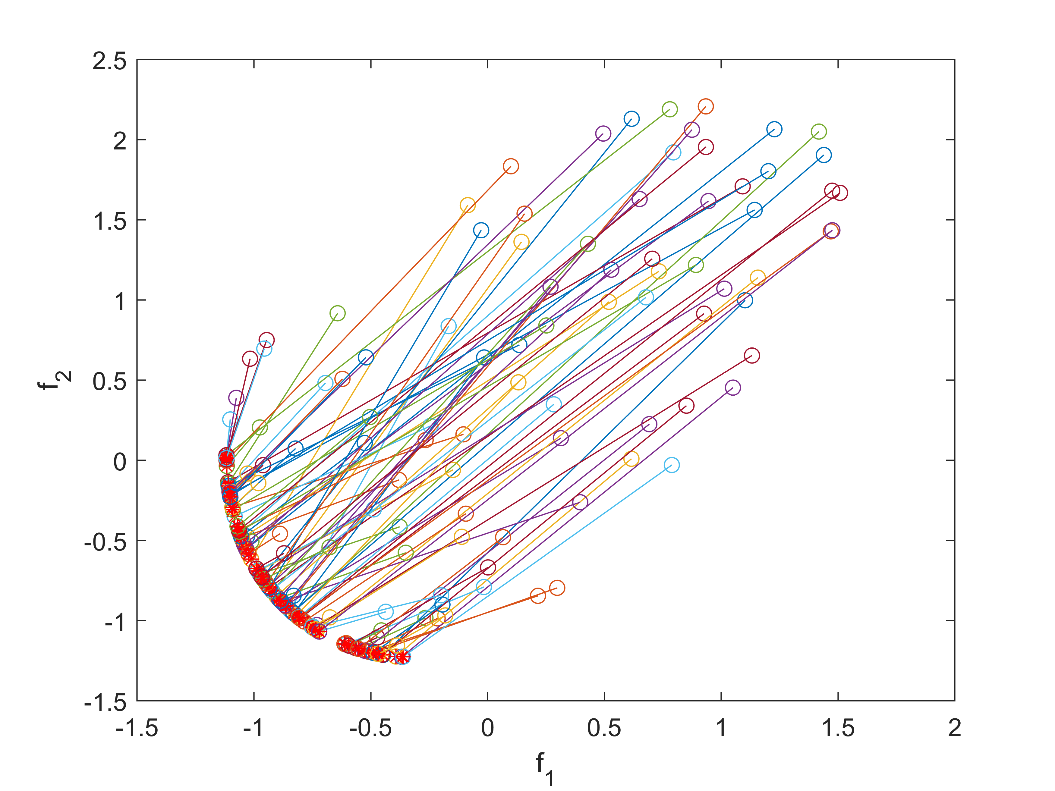
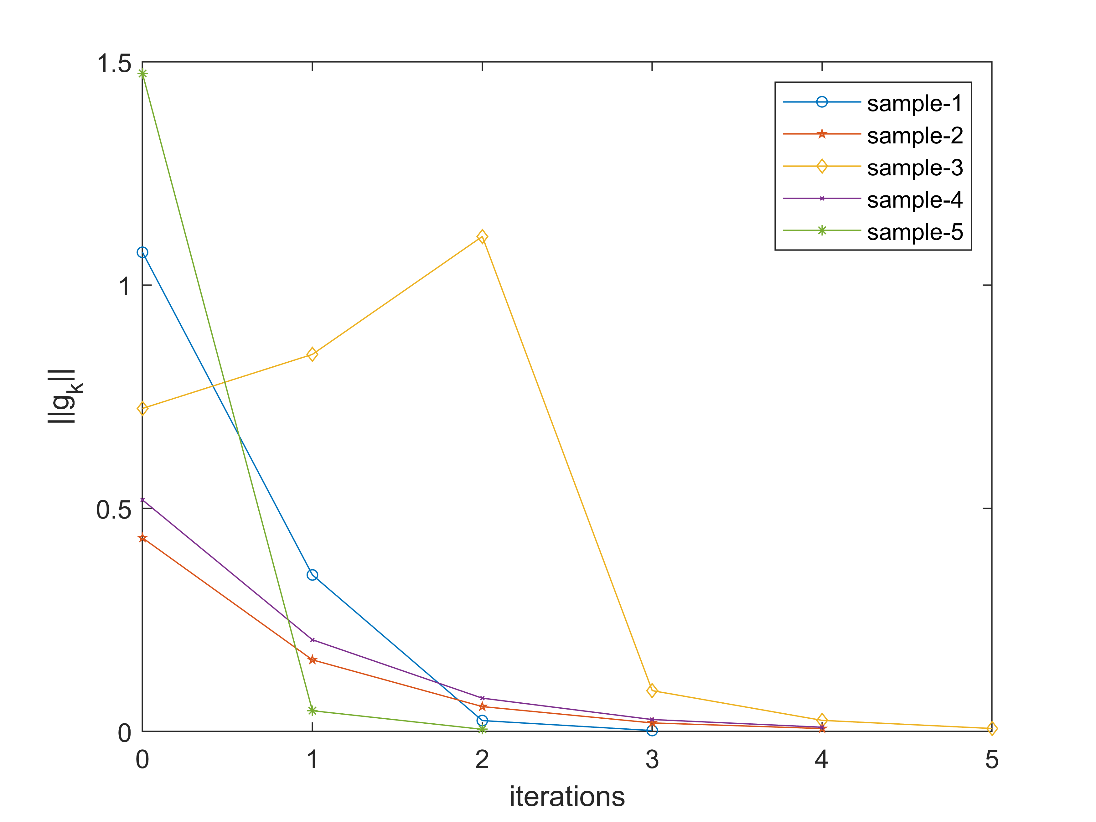
Figure 1: Numerical results for Example 1.

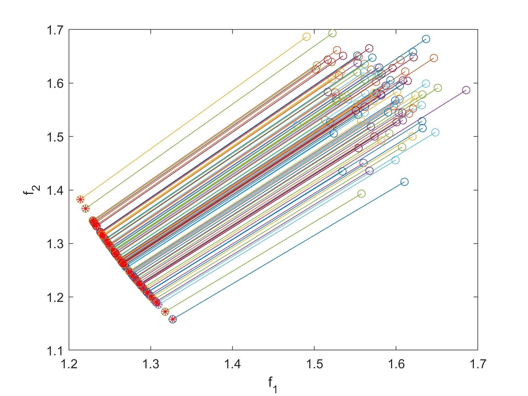
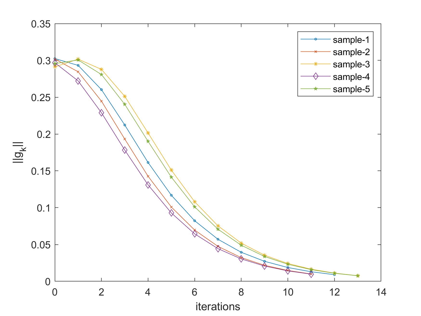
Figure 2: Numerical results for Example 2 with $m=2$.

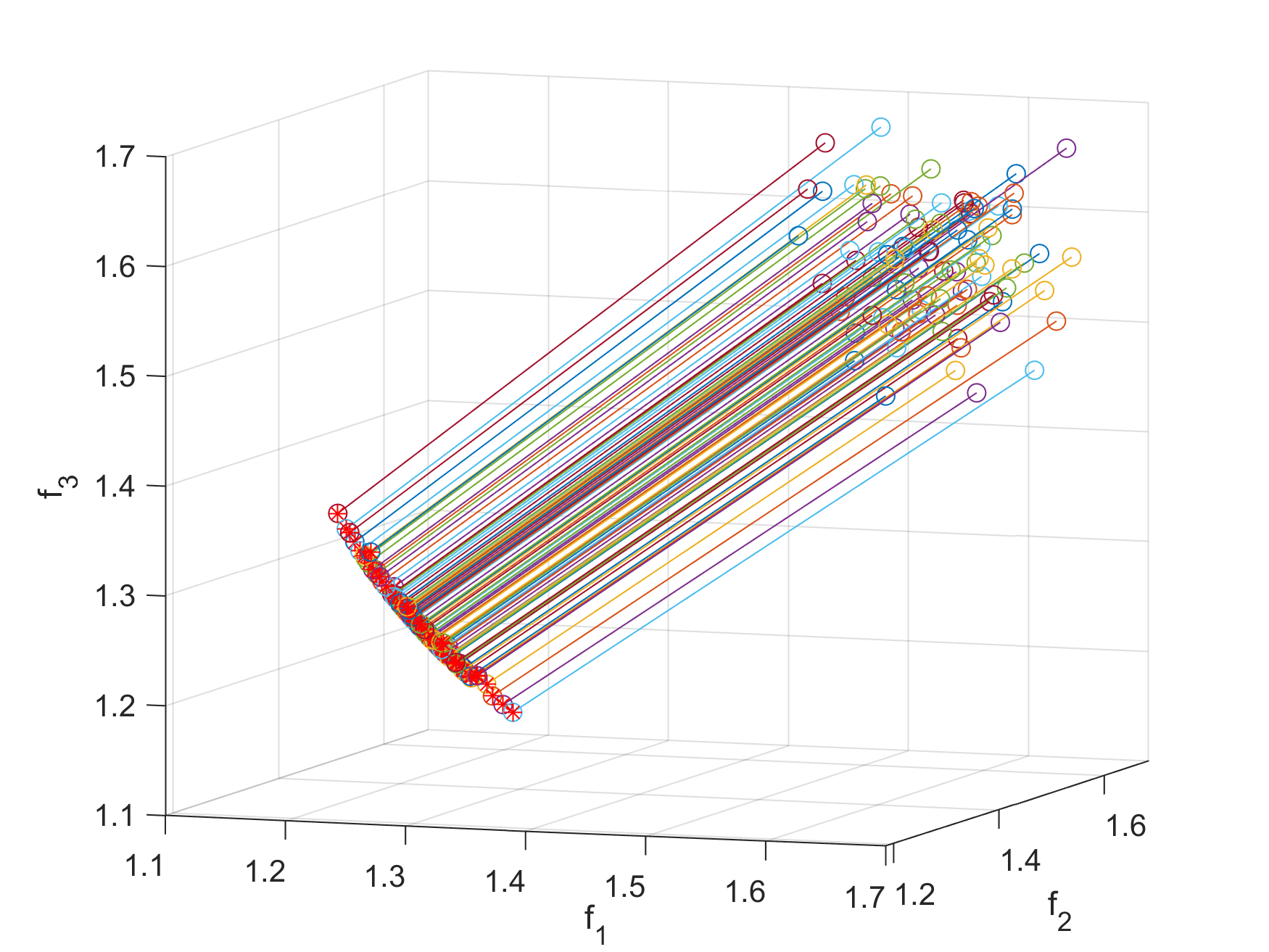
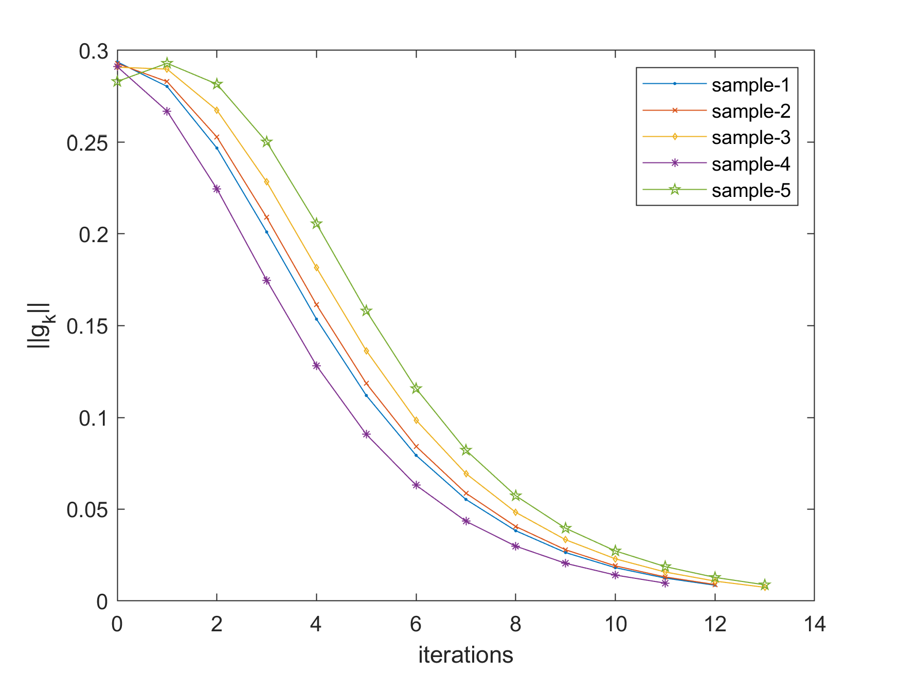
Figure 3: Numerical results for Example 2 with $m=3$.

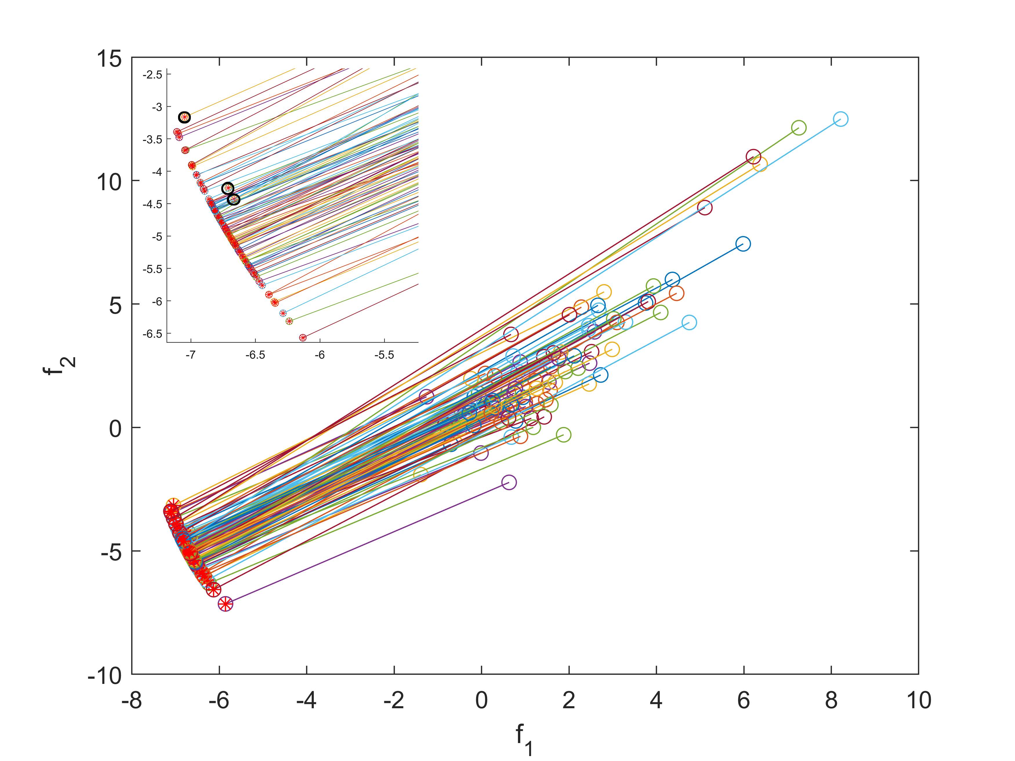
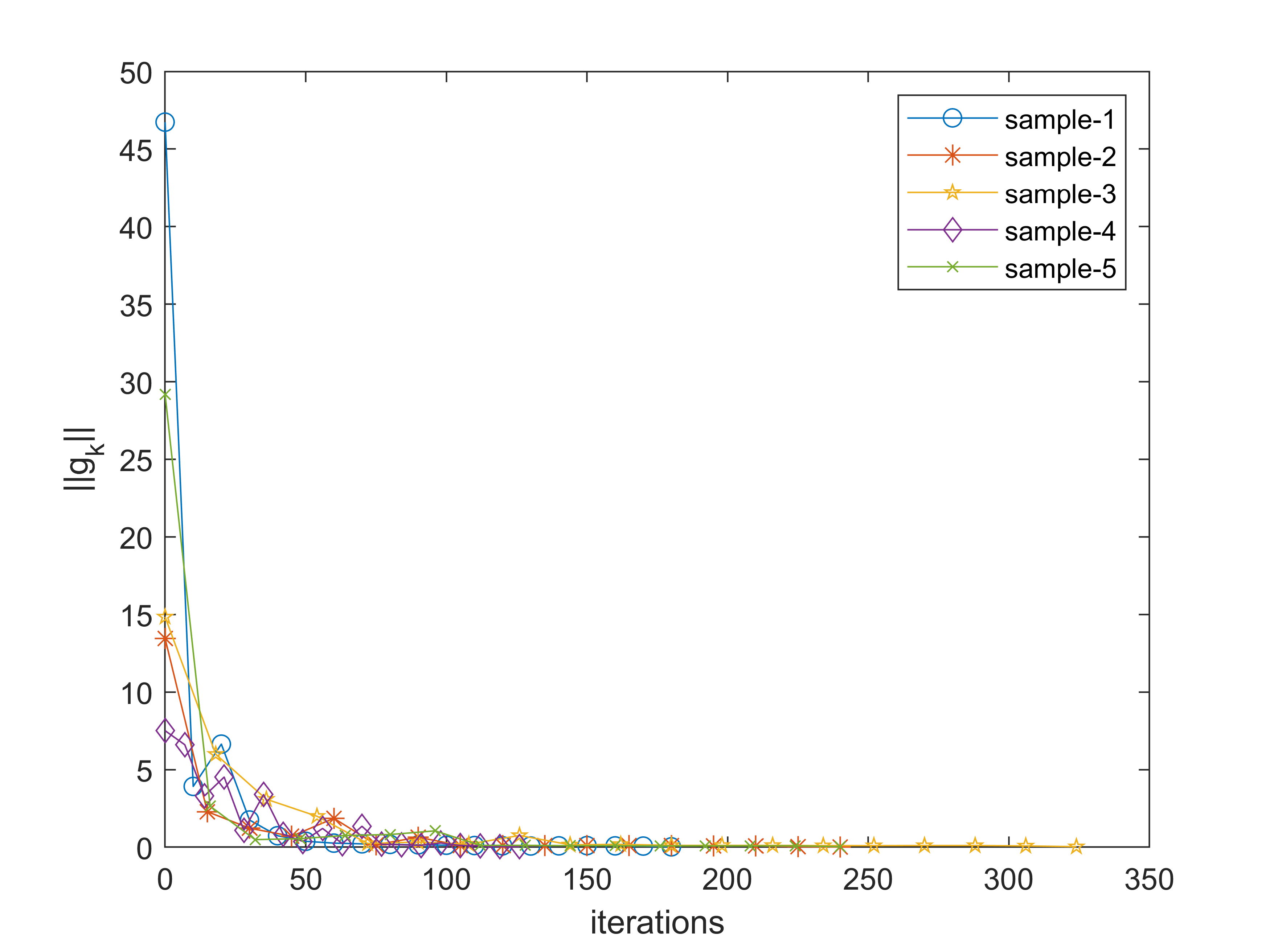
Figure 4: Numerical results for Example 3 with $p=100$, $m=2$, and $A_{i}$ being randomly generated for $i=1,2$.

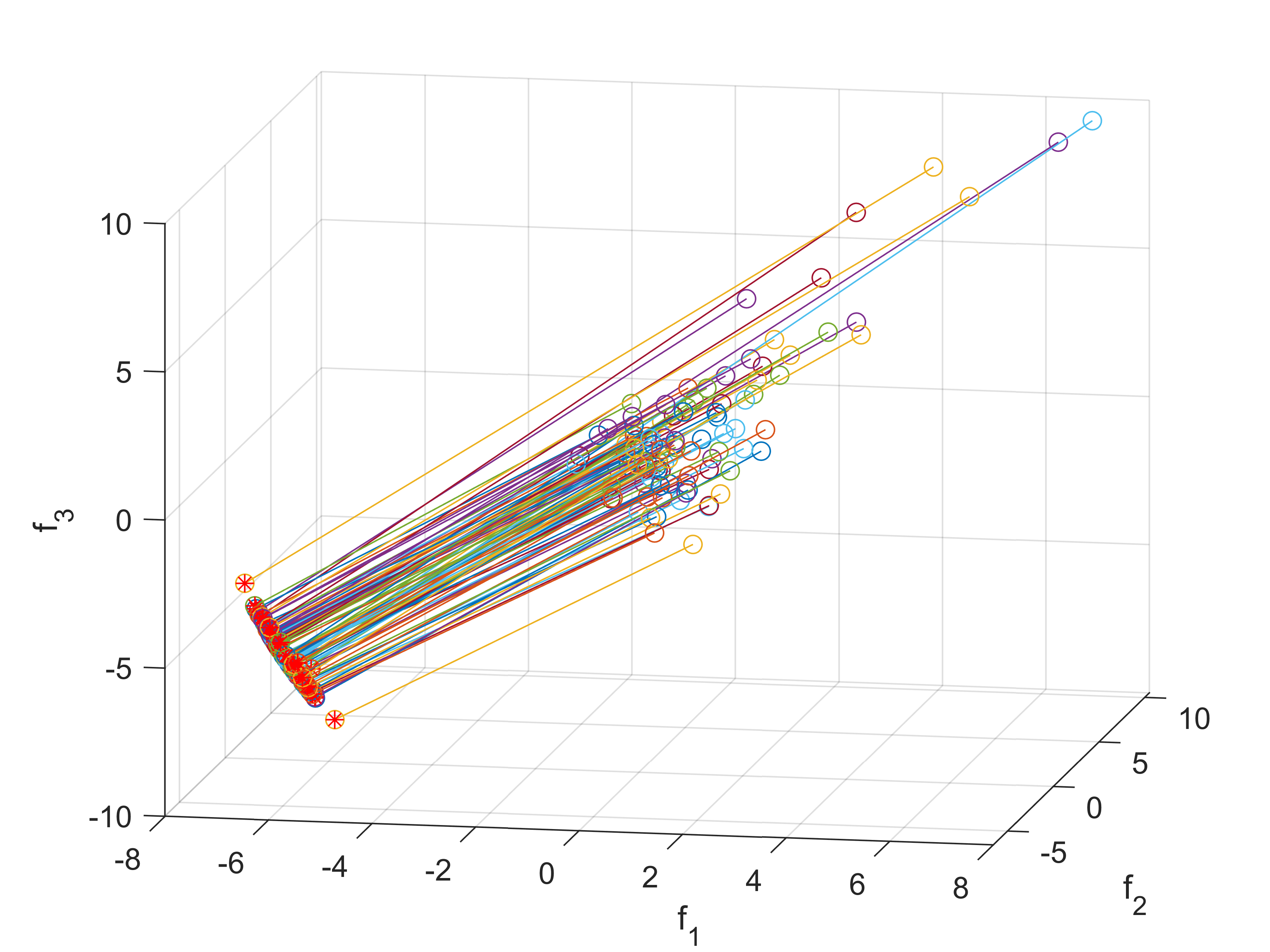
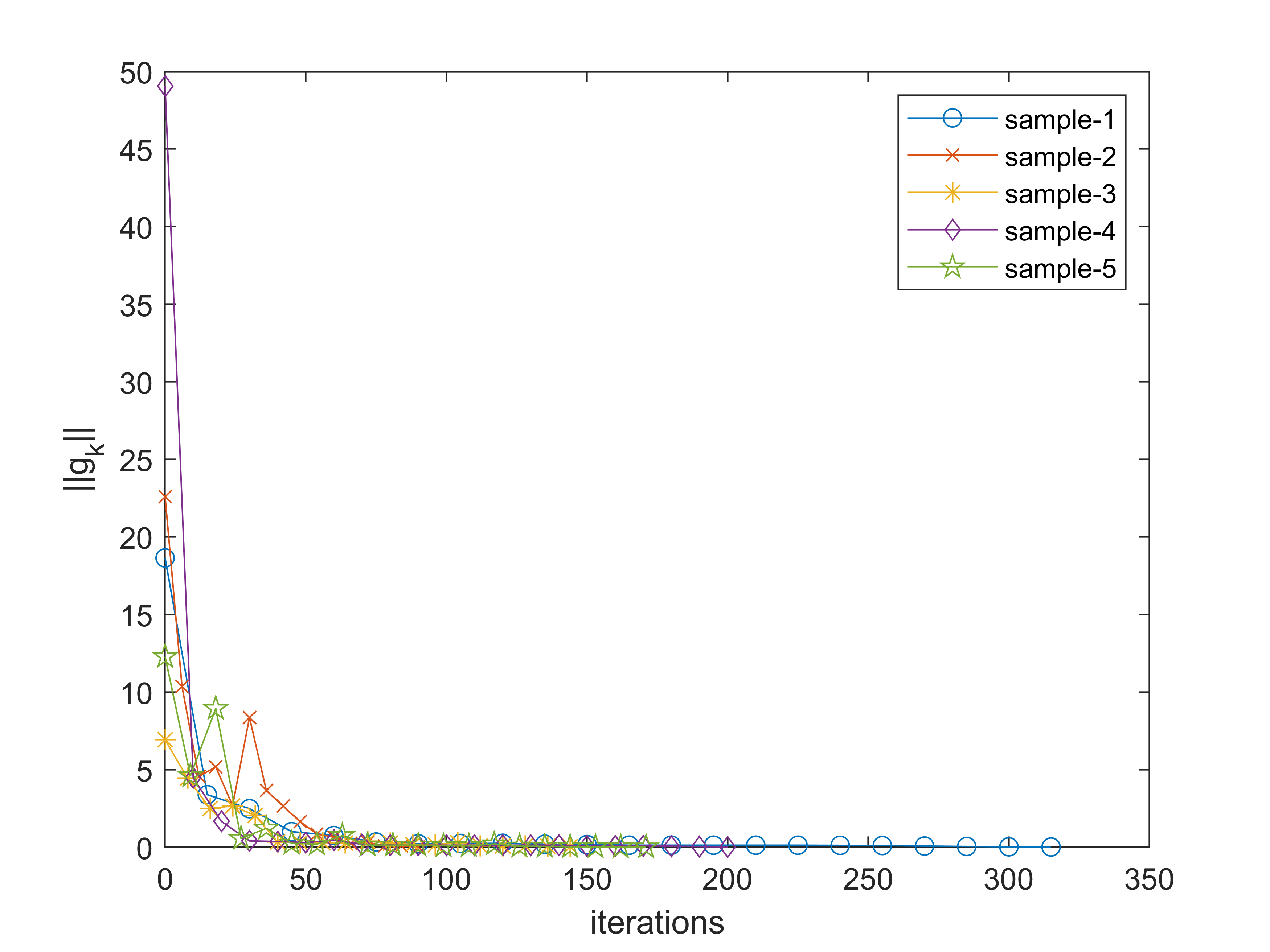
Figure 5: Numerical results for Example 3 with $p=100$, $m=3$, and $A_{i}$ being randomly generated for $i=1,2,3$.

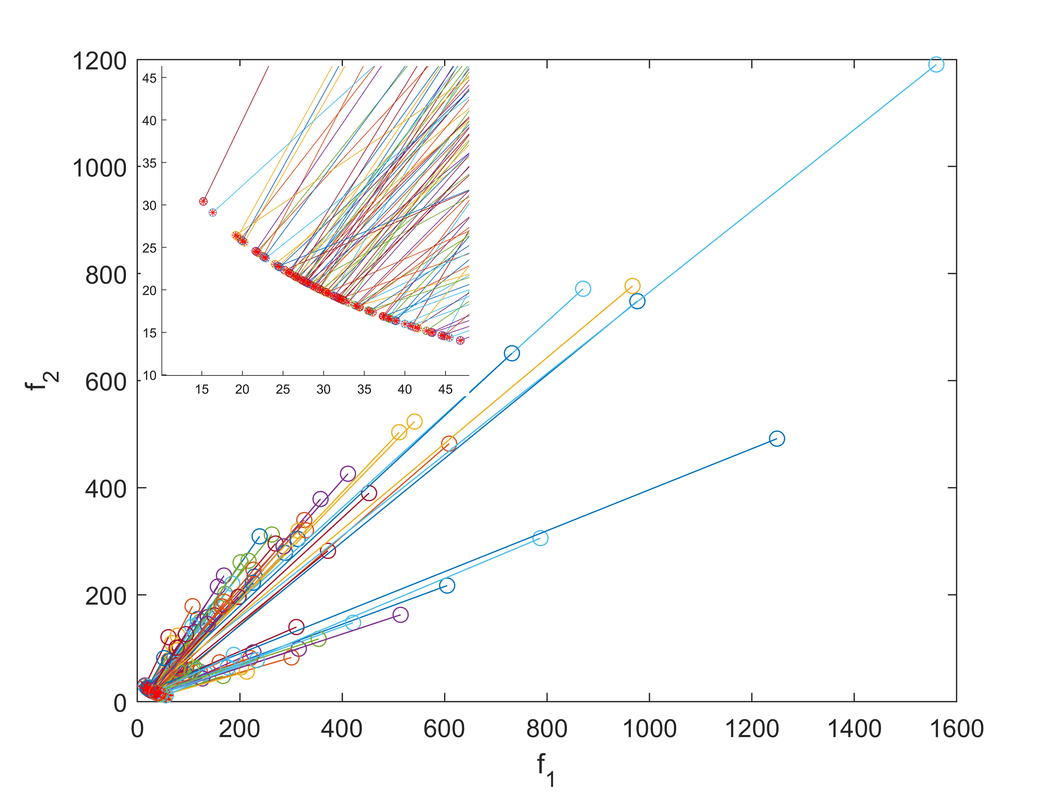
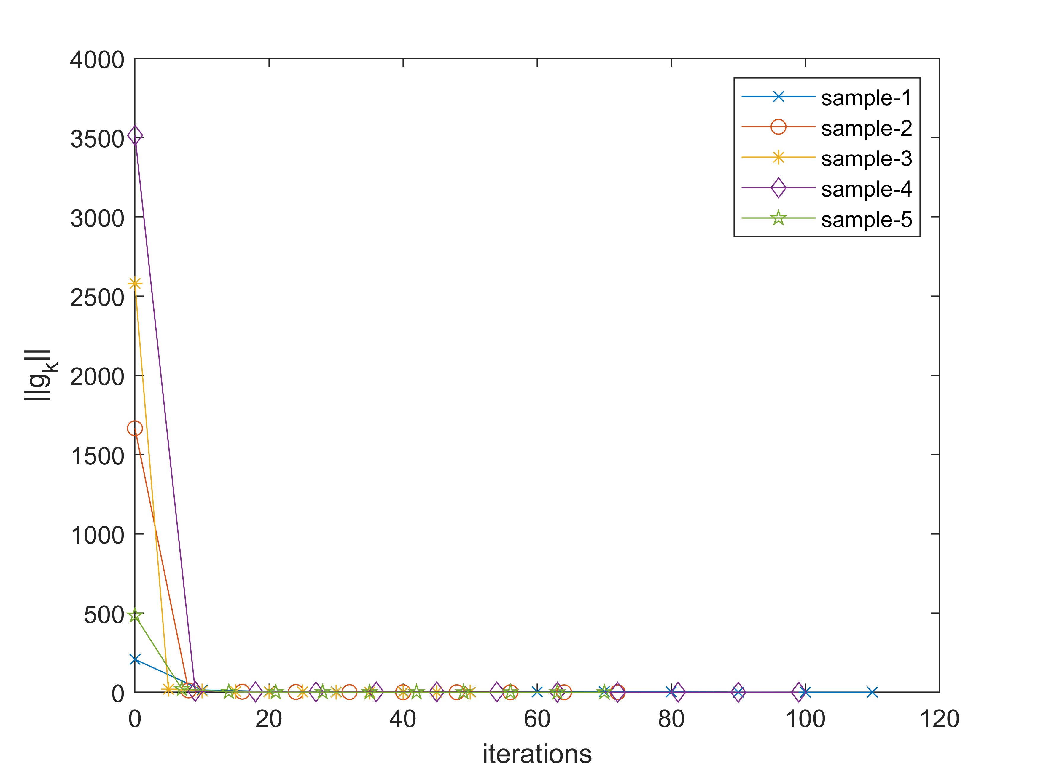
Figure 6: Numerical results for Example 4 with $n=100$, $p=60$, $m=2$, $\lambda_{1}=0.01$, $\lambda_{2}=0.02$, $A_{i}$ and $b_{i}$ being randomly generated for $i=1,2$.

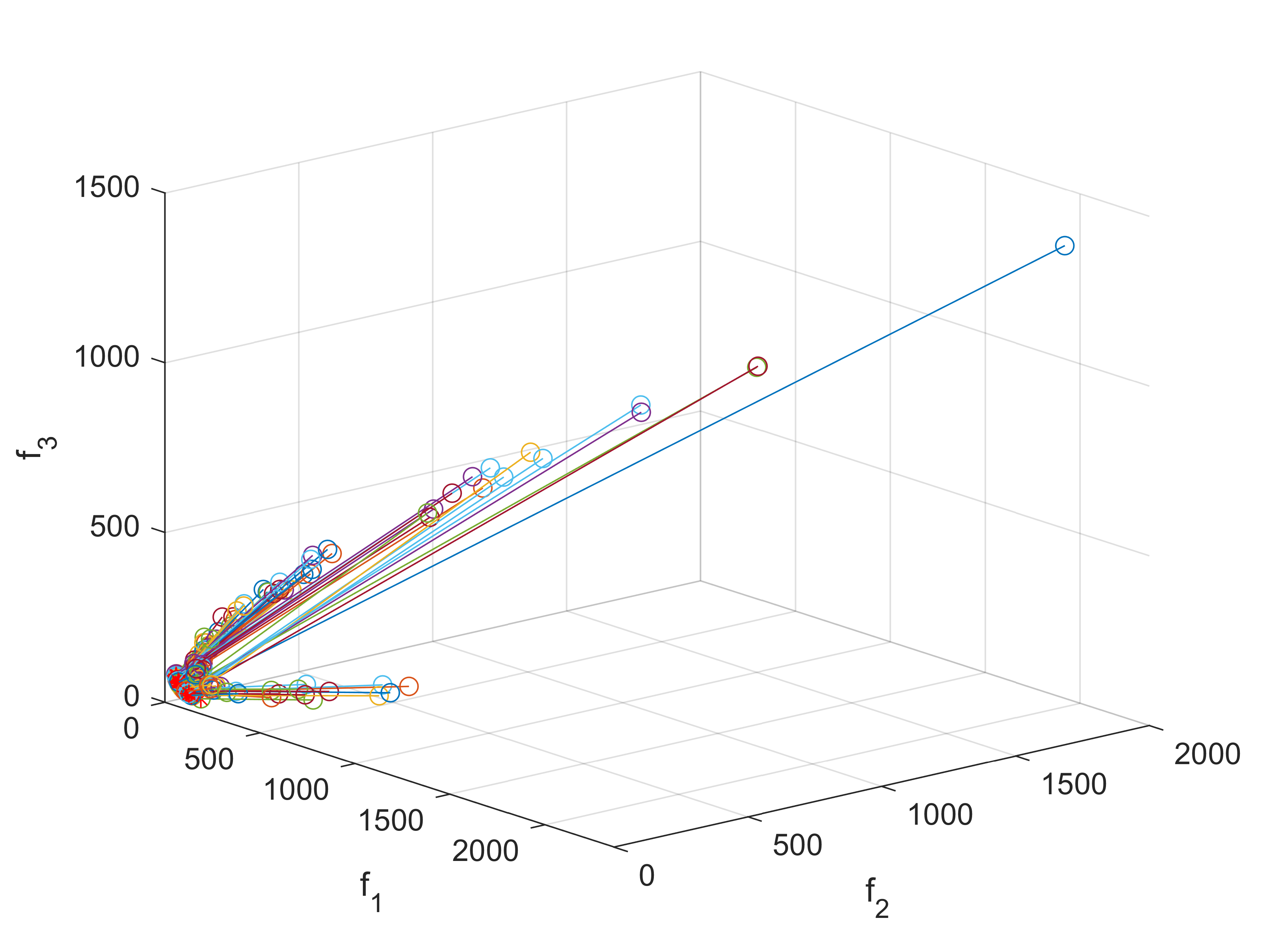
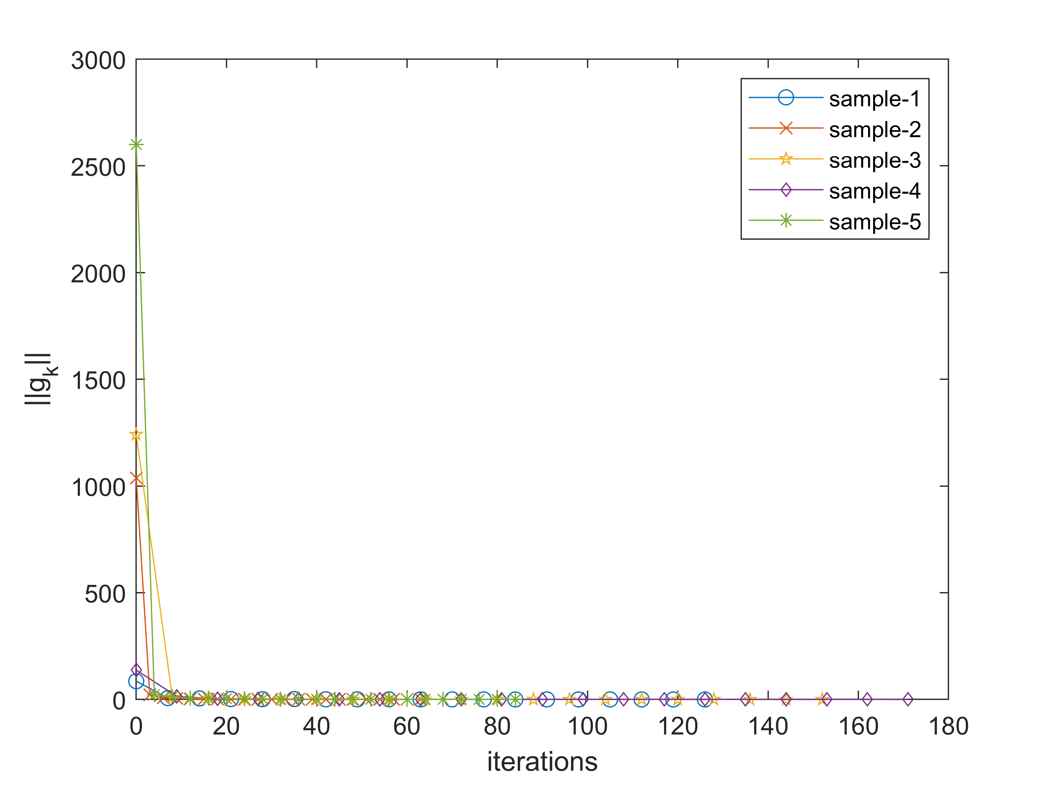
Figure 7: Numerical results for Example 4 with $n=100$, $p=60$, $m=3$, $\lambda_{1}=0.01$, $\lambda_{2}=0.02$, $\lambda_{3}=0.02$, $A_{i}$ and $b_{i}$ being randomly generated for $i=1,2,3$.

In Figs. 1–7, the hollow points indicate the objective vector values of the initial points, and these marked with red stars are the objective vector values of the final points (namely, the $(\varepsilon,\delta)$-critical points). From these figures, we see that nearly all of the final points generated by our method are (approximate) Pareto optimal points for the corresponding examples, except that several points marked with black circles in Fig. 4 are not Pareto optimal, which might be local (weak) Pareto optimal points. Thus, we can obtain the approximations of Pareto sets for the above examples by Algorithm 1 when some reasonable number of starting points are given. Furthermore, in Table 1, we list the average number of iterations (ANI) for $100$ random starting points for all examples. In summary, the preliminary numerical results show that our method is effective and promising.

Table 1: Average number of iterations

Example	1	2 ($m=2$)	2 ($m=3$)	3 ($m=2$)	3 ($m=3$)	4 ($m=2$)	4 ($m=3$)
ANI	4.4	13.0	13.0	266.3	192.4	98.8	102.1

6 Conclusions

In this paper, we have presented a descent method for multiobjective optimization problems with locally Lipschitz components on complete Riemannian manifolds. Our setting is much more general than certain convexities assumed in the existing works. To avoid computing the Riemannian $\varepsilon$-subdifferential of the objective vector function, a convex hull of some Riemannian $\varepsilon$-subgradients is constructed to obtain an acceptable descent direction, which greatly reduces the computational complexity. Furthermore, we extend a necessary condition of the Pareto optimal points to the Riemannian setting. Finite convergence of the proposed algorithm is obtained under the assumption that at least one objective function is bounded below and the employed retraction and vector transport satisfy certain conditions. Finally, some preliminary numerical results illustrate the effectiveness of our method. As a future work, similar to the idea in Hosseini2 , we may further extend the norm in (12) by the $P$-norm and choose the direction as $P\tilde{g}$, where $P$ is a positive definite matrix.

$\mathbf{Funding}$ This work was supported by the National Natural Science Foundation of China (12271113, 12171106, 12061013) and Guangxi Natural Science Foundation (2020GXNSFDA238017).

$\mathbf{Data\,\,availability}$ The datasets generated and analysed during the current study are available from the corresponding author on reasonable request.

References

- (1) Abraham, A., Jain, L.: Evolutionary Multiobjective Optimization. Springer (2005)
- (2) Absil, P.A., Mahony, R., Sepulchre, R.: Optimization Algorithms on Matrix Manifolds. Princeton University Press (2008)
- (3) Attouch, H., Garrigos, G., Goudou, X.: A dynamic gradient approach to Pareto optimization with nonsmooth convex objective functions. J. Math. Anal. Appl. (1), 741-771 (2015)
- (4) Bagchi, U.: Simultaneous minimization of mean and variation of flow time and waiting time in single machine systems. Oper. Res. (1), 118-125 (1989)
- (5) Boumal, N.: An Introduction to Optimization on Smooth Manifolds. Cambridge University Press (2023)
- (6) Bento, G.C., Cruz Neto, J.X.: A subgradient method for multiobjective optimization on Riemannian manifolds. J. Optim. Theory Appl. (1), 125-137 (2013)
- (7) Bento, G.C., Melo, J.G.: Subgradient method for convex feasibility on Riemannian manifolds. J. Optim. Theory Appl. (3), 773-785 (2012)
- (8) Bonnel, H., Iusem, A.N., Svaiter, B.F.: Proximal methods in vector optimization. SIAM J. Optim. (4), 953-970 (2005)
- (9) Bento, G.C., Ferreira, O.P., Oliveira, P.R.: Unconstrained steepest descent method for multicriteria optimization on Riemannian manifolds. J. Optim. Theory Appl. , 88-107 (2012)
- (10) Bento, G.C., Cruz Neto, J.X., Santos, P.S.M: An inexact steepest descent method for multicriteria optimization on Riemannian manifolds. J. Optim. Theory Appl. , 108-124 (2013)
- (11) Bento, G.C., Cruz Neto, J.X., Lpez, G., Soubeyran, A., Souza, J.C.O.: The proximal point method for locally Lipschitz functions in multiobjective optimization with application to the compromise problem. SIAM J. Optim. (2), 1104-1120 (2018)
- (12) Bento, G.C., Cruz Neto, J.X., Meireles, L.V.: Proximal point method for locally Lipschitz functions in multiobjective optimization of Hadamard manifolds. J. Optim. Theory Appl. , 37-52 (2018)
- (13) Clarke, F.: Optimization and Nonsmooth Analysis. Society for Industrial and Applied Mathematics (1983)
- (14) Deb, K.: Multi-objective optimisation using evolutionary algorithms: an introduction. Springer (2011)
- (15) Ehrgott, M.: Multicriteria Optimization. Springer, New York (2005)
- (16) El Moudden, M., El Mouatasim, A.: Accelerated diagonal steepest descent method for unconstrained multiobjective optimization. J. Optim. Theory Appl. (1), 220-242 (2021)
- (17) Engau, A., Wiecek, M.M.: 2D decision-making for multicriteria design optimization. Structural and Multidisciplinary Optimization. , 301-315 (2007)
- (18) Eslami, N., Najafi, B., Vaezpour, S.M.: A trust region method for solving multicriteria optimization problems on Riemannian manifolds. J. Optim. Theory Appl. (1), 212-239 (2023)
- (19) Fliege, J.: OLAF-a general modeling system to evaluate and optimize the location of an air polluting facility. OR Spektrum. (1), 117–136 (2001)
- (20) Fliege, J., Svaiter, B.F.: Steepest descent methods for multicriteria optimization. Math. Methods Oper. Res. (3), 479-494 (2000)
- (21) Fliege, J., Drummond, L.G., Svaiter, B.F.: Newton’s method for multiobjective optimization. SIAM J. Optim. (2), 602-626 (2009)
- (22) Fletcher, P. T., Venkatasubramanian, S., Joshi, S.: The geometric median on Riemannian manifolds with application to robust atlas estimation. NeuroImage. (1), S143-S152 (2009)
- (23) Geoffrion, A.M.: Proper efficiency and the theory of vector maximization. J. Math. Anal. Appl. (3), 618-630 (1968)
- (24) Gebken, B., Peitz, S.: An efficient descent method for locally Lipschitz multiobjective optimization problems. J. Optim. Theory Appl. (3), 696-723 (2021)
- (25) Gravel, M., Martel, J.M., Madeau, R., Price, W., Tremblay, R.: A multicriterion view of optimal ressource allocation in job-shop production. Eur. J. Oper. Res. (1-2), 230-244 (1992)
- (26) Hosseini, S., Pouryayevali, M.R.: Generalized gradients and characterization of epi-Lipschitz sets in Riemannian manifolds. Nonlinear Anal. (12), 3884-3895 (2011)
- (27) Hosseini, S., Uschmajew, A.: A Riemannian gradient sampling algorithm for nonsmooth optimization on manifolds. SIAM J. Optim. (1), 173-189 (2017)
- (28) Huang, W., Gallivan, K.A., Absil, P.A.: A Broyden class of quasi-Newton methods for Riemannian optimization. SIAM J. Optim. (3), 1660-1685 (2015)
- (29) Hosseini, S., Huang, W., Yousefpour, R.: Line search algorithms for locally Lipschitz functions on Riemannian manifolds. SIAM J. Optim. (1), 596-619 (2018)
- (30) Hu, J., Liu, X., Wen, Z.W., Yuan, Y.X.: A brief introduction to manifold optimization. J. Oper. Res. Soc. China (2), 199-248 (2020)
- (31) Hoseini Monjezi, N., Nobakhtian, S., Pouryayevali, M.R.: A proximal bundle algorithm for nonsmooth optimization on Riemannian manifolds. IMA J. Numer. Anal. (1), 293-325 (2023)
- (32) Leschine, T.M., Wallenius, H., Verdini, W.A.: Interactive multiobjective analysis and assimilative capacity-based ocean disposal decisions. Eur. J. Oper. Res. (2), 278-289 (1992)
- (33) Mahdavi-Amiri, N., Yousefpour, R.: An effective nonsmooth optimization algorithm for locally Lipschitz functions. J. Optim. Theory Appl. , 180-195 (2012)
- (34) Mäkelä, M.M., Eronen, V.P., Karmitsa, N.: On Nonsmooth Multiobjective Optimality Conditions with Generalized Convexities, pp. 333–357. Springer, New York (2014)
- (35) Mäkelä, M.M., Karmitsa, N., Wilppu, O.: Proximal bundle method for nonsmooth and nonconvex multiobjective optimization. Mathematical modeling and optimization of complex structures, pp. 191-204. Springer (2016)
- (36) Povalej, Ž.: Quasi-Newton’s method for multiobjective optimization. J. Comput. Appl. Math. , 765-777 (2014)
- (37) Sato, H.: Riemannian Optimization and Its Applications. Springer Nature, Switzerland (2021)
- (38) Sawaragi, Y., Nakayama, H., Tanino, T.: Theory of multiobjective optimization. Elsevier (1985).
- (39) Tibshirani, R.: Regression shrinkage and selection via the lasso. J. R. Stat. Soc. Ser. B. (1), 267-288 (1996)
- (40) Zhu, X.: A Riemannian conjugate gradient method for optimization on the Stiefel manifold. Comput. Optim. Appl. , 73-110 (2017)