Towards Mode Balancing of Generative Models via Diversity Weights

Abstract

Large data-driven image models are extensively used to support creative and artistic work. Under the currently predominant distribution-fitting paradigm, a dataset is treated as ground truth to be approximated as closely as possible. Yet, many creative applications demand a diverse range of output, and creators often strive to actively diverge from a given data distribution. We argue that an adjustment of modelling objectives, from pure mode coverage towards mode balancing, is necessary to accommodate the goal of higher output diversity. We present diversity weights, a training scheme that increases a model’s output diversity by balancing the modes in the training dataset. First experiments in a controlled setting demonstrate the potential of our method. We discuss connections of our approach to diversity, equity, and inclusion in generative machine learning more generally, and CC specifically. An implementation of our algorithm is available at https://github.com/sebastianberns/diversity-weights

Introduction

LIGM, in particular as part of text-to-image generation systems (Ramesh et al., 2021; Saharia et al., 2022), have been widely adopted by visual artists to support their creative work in art production, ideation, and visualisation (Ko et al., 2023; Vimpari et al., 2023). While providing vast possibility spaces, large image generation models, trained on huge image datasets scraped from the internet, not only adopt but often exacerbate data biases, as observed in word embedding and captioning models (Bolukbasi et al., 2016; Zhao et al., 2017; Hendricks et al., 2018). The tendency to emphasise majority features and to primarily reproduce the predominant types of data examples can be limiting for many computational creativity (CC) applications that use machine learning-based generators (Loughran and O’Neill, 2017). Learned models are often used to illuminate a possibility space and to produce artefacts for further design iterations. Examples range from artistic creativity, like the production of video game assets (Liapis, Yannakakis, and Togelius, 2014; Volz et al., 2018), over constrained creativity, e.g. industrial design and architecture (Bradner, Iorio, and Davis, 2014), to scientific creativity, such as drug discovery (Madani et al., 2023). Many of these and similar applications would benefit from higher diversity in model output. Given that novelty, which underlies diversity, is considered one of the essential aspects of creativity (Boden, 2004; Runco and Jaeger, 2012), we expect that, vice versa, a stronger focus on diversity can also foster creativity (cf. Stanley and Lehman, 2015).

Most common modelling techniques, however, follow a distribution-fitting paradigm and do not accommodate the goal of higher diversity. Within this paradigm, one of the primary generative modelling objectives is mode coverage (Zhong et al., 2019), i.e. the capability of a model to generate all prominent types of examples present in a dataset. While such a model can in principle produce many types of artefacts, it does not do so reliably or evenly. A model’s probability mass is assigned in accordance to the prevalence of a type of example or feature in a dataset. Common examples or features have higher likelihood under the model than rare ones. As a consequence, samples with minority features are not only less likely to be obtained by randomly sampling a model, they are also of lower fidelity, e.g. in terms of image quality. Related studies on Transformer-based language models (Razeghi et al., 2022; Kandpal, Wallace, and Raffel, 2022) have identified a “superlinear” relationship: while training examples with multiple duplicates are generated “dramatically more frequently”, examples that only appear once in the dataset are rarely reproduced by the model.

In this work, we argue for an adjustment of modelling techniques from mode coverage to mode balancing to enrich CC with higher output diversity. Our approach allows to train models that cover all types of training examples and can generate them with even probability and fidelity. We present a two-step training scheme designed to reliably increase output diversity. Our technical contributions are:

• Diversity weights, a training scheme to increase a generative model’s output diversity by taking into account the relative contribution of individual training examples to overall diversity.

• Weighted Fréchet Inception Distance (wFID), an adaptation of the FID measure to estimate the distance between a model distribution and a target distribution modified by weights over individual training examples.

• A proof-of-concept study, demonstrating the capacity of our method to increase diversity, examining the trade-off between artefact typicality and diversity.

In the following sections, we first introduce the objective of mode balancing and highlight its importance for CC based on existing frameworks and theories. Then, we provide background information on the techniques relevant for our work. Next, we present our diversity weights method in detail, as well as our formulation of Weighted FID. Following this, we present the setup and methodology of our study and evaluate its results. In the discussion section, we contribute to the debate on issues of diversity, equity, and inclusion (DEI) in generative machine learning more generally, and CC specifically, by explaining how our method could be beneficial in addressing data imbalance bias. This is followed by an overview of related work, our conclusions and an outlook on future work.

Mode Balancing

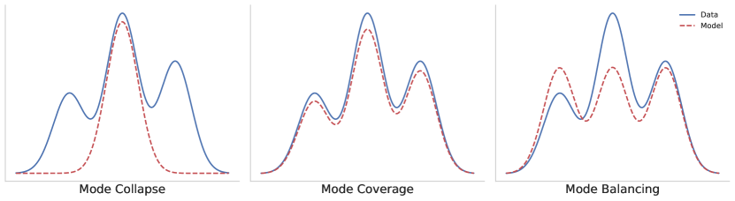
Figure 1: Mode collapse: the model does not cover all modes in the data distribution. Mode coverage: the data distribution’s modes are modelled as closely as possible w.r.t. their likelihood. Mode balancing: the model covers all modes, but with equal likelihood.

Generative deep learning models now form an integral part of CC systems (Berns et al., 2021). A lot of work on such models is concerned with mode coverage: to match a data distribution as closely as possible by accurately modelling all types of examples in a dataset (fig. 1). In the specific case of generative adversarial networks, great effort is put into preventing mode collapse, a training failure state in which a model disregards important modes and is only able to produce a few types of training examples. Mode coverage is captured formally in common evaluation measures such as Fréchet Inception Distance (FID) and Precision–Recall (PR). Crucially, this is always done in reference to the training set statistics or data manifold. In this context, diversity is often arguably misused to refer to mode coverage. While mode coverage describes the fraction of modes in a dataset that are represented by a model, the diversity of a model’s output, if understood more generally and intuitively, can theoretically be higher than that of the dataset.

Mode coverage is conceptually similar to the notion of typicality (Ritchie, 2007). Defined as the extent to which a produced output is “an example of the artefact class in question”, a model which only generates outputs with high typicality, if sampled at random, has to provide most support to those training set examples with the highest density of features characteristic of that artefact, i.e. to maximise mode coverage. Crucially, sampling from the model would resemble going along the most well-trodden paths in the possibility space defined by the dataset and, as Ritchie already suggests, counteract novelty as a core component of creativity (Boden, 2004; Runco and Jaeger, 2012).

Crucially, mode balancing breaks with the convention of viewing the dataset as ‘ground truth’. Instead, we consider the dataset to provide useful domain information and the characteristics of typical examples (Ritchie, 2007). But a data distribution does not have to be matched exactly. Particularly in artistic applications, creators often strive to actively diverge from the typical examples in a dataset (Berns and Colton, 2020; Broad et al., 2021). To stay with our metaphor, borrowed from Veale, Cardoso, and Pérez y Pérez (2019), mode balancing allows us to walk more along the less trodden paths and thus especially support exploratory and transformational creativity (Boden, 2004; Stanley and Lehman, 2015). In contrast to the mode coverage paradigm, in mode balancing, diversity is measured independently of the training data distribution. In the theoretical case of a balanced dataset of absolutely dissimilar examples, i.e. multiple equally likely modes, our method would assign uniform weights to all examples and thus be identical to standard training schemes with random sampling.

Background

Probability-Weighted Vendi Score

We adopt the Vendi Score (VS) as a measure of dataset diversity and employ its probability-weighted formulation in our work (Friedman and Dieng, 2022). Given a set of artefacts $x_{1},\dots,x_{n}$, the probability-weighted VS is based on a probability vector $\boldsymbol{\mathbf{p}}=(p_{1},\dots,p_{n})$ and a similarity matrix $\boldsymbol{\mathbf{K}}\in\mathbb{R}^{\,n\times n}$ between pairs of artefacts such that $\boldsymbol{\mathbf{K}}_{ii}=1$. Calculating VS involves various steps. First, the probability-weighted similarity matrix is defined as $\boldsymbol{\mathbf{K}}^{\boldsymbol{\mathbf{p}}}=\textrm{diag}(\sqrt{\boldsymbol{\mathbf{p}}})\,\boldsymbol{\mathbf{K}}\,\textrm{diag}(\sqrt{\boldsymbol{\mathbf{p}}})$. Its eigenvectors $\lambda_{1},\dots,\lambda_{n}$ can be obtained via the eigendecomposition $\boldsymbol{\mathbf{K}}^{\boldsymbol{\mathbf{p}}}=\boldsymbol{\mathbf{Q}}\boldsymbol{\mathbf{\Lambda}}\boldsymbol{\mathbf{Q}}^{-1}$, where $\boldsymbol{\mathbf{\lambda}}=\textrm{diag}(\boldsymbol{\mathbf{\Lambda}})$. The probability-weighted Vendi Score (VS) is the exponential of the Shannon entropy of the eigenvalues of the probability-weighted similarity matrix:

$$\textrm{VS}(\boldsymbol{\mathbf{K}},\boldsymbol{\mathbf{p}})=\exp\Big{(}-\sum^{n}\lambda_{i}\,\log\lambda_{i}\Big{)}$$ (1)

Also known as perplexity, exponential entropy can be used to measure how well a probability model predicts a sample. Low perplexity indicates good prediction performance. Consequently, the more diverse a sample, the more difficult its prediction, the higher the perplexity and its VS.

Illustrative Example

The probability vector $p$ represents the relative abundances of individual artefacts. Instead of repeating identical artefacts in a set, their prevalence can be expressed with higher probability. For illustration, we present an example of four artefacts, of which three are absolutely similar to each other and one is absolutely dissimilar to all others. All have equal probability.

$$\boldsymbol{\mathbf{K}}^{a}=\begin{pmatrix}1&0&0&0\\ 0&1&1&1\\ 0&1&1&1\\ 0&1&1&1\\ \end{pmatrix},\quad\boldsymbol{\mathbf{p}}^{a}=\begin{pmatrix}0.25\\ 0.25\\ 0.25\\ 0.25\\ \end{pmatrix}$$ (2)

The same information can be reduced to two absolutely dissimilar artefacts and the corresponding probabilities $\boldsymbol{\mathbf{p}}^{b}$.

$$\boldsymbol{\mathbf{K}}^{b}=\begin{pmatrix}1&0\\ 0&1\\ \end{pmatrix},\quad\boldsymbol{\mathbf{p}}^{b}=\begin{pmatrix}0.25\\ 0.75\\ \end{pmatrix}$$ (3)

Both representations yield the same VS, which reflects the imbalanced set of two absolutely dissimilar artefacts. $\textrm{VS}(\boldsymbol{\mathbf{K}}^{a},\boldsymbol{\mathbf{p}}^{a})=\textrm{VS}(\boldsymbol{\mathbf{K}}^{b},\boldsymbol{\mathbf{p}}^{b})=1.755\dots$

The imbalance of our example set negatively affects its diversity. If all items in the set are given equal importance, one artefact is under-represented. Instead, each of the two absolutely dissimilar artefacts in the set should thus be assigned equal weight $p=0.5$. In the case of repetitions, this weight has to be divided across the repeated artefacts.

$$\boldsymbol{\mathbf{K}}^{c}=\begin{pmatrix}1&0&0&0\\ 0&1&1&1\\ 0&1&1&1\\ 0&1&1&1\\ \end{pmatrix},\quad\boldsymbol{\mathbf{p}}^{c}=\begin{pmatrix}0.5\\ 0.166\dots\\ 0.166\dots\\ 0.166\dots\\ \end{pmatrix}$$ (4)

This maximises VS to reflect the effective number of absolutely dissimilar artefacts $\textrm{VS}(\boldsymbol{\mathbf{K}}^{c},\boldsymbol{\mathbf{p}}^{c})=2$.

Importance Sampling

Conventionally, training examples are drawn from a dataset with uniform probability. In importance sampling, instead, examples are chosen according to their contribution to an unknown target distribution. In our case, the importance of training examples is determined by their individual contribution to the overall dataset diversity as quantified by the optimised probability distribution $p$ (see example above). We aim to increase the output diversity of a model. For this, we replace the basic sampling operation by a diversity-weighted importance sampling scheme.

Model Evaluation

To assess model performance, we use some common measures for generative models, as well as measures specifically relevant to our method. Inception Score (IS) (Salimans et al., 2016), Fréchet Inception Distance (FID) (Heusel et al., 2017), and Precision-Recall (k-NN parameter $k=3$) (Kynkäänniemi et al., 2019) quantify sample fidelity and mode coverage w.r.t. the unbiased training data distribution. We employ our Weighted Fréchet Inception Distance (wFID) to account for the change in target distribution, induced by our method through diversity-weighted sampling (see below for details). Diversity is estimated with the Vendi Score (VS) (Friedman and Dieng, 2022).

Note that we follow the recommendations by Barratt and Sharma (2018) and calculate IS over the entire generated set of samples, removing the common split into subsets. We also remove the exponential, such that the score becomes interpretable in terms of mutual information. While not all reported scores are directly comparable to other works, our measurements are internally consistent and reliable.

Image Embeddings

Instead of comparing image data on raw pixels, standard evaluation measures of model performance have relied on image classification networks to be used as embedding models for feature extraction. The InceptionV3 model (Szegedy et al., 2016) is most commonly used as a representative feature space and has been widely adopted as part of a standard measurement pipeline. Unfortunately, small numerical differences in model weights, implementations and interpolation operations can compound to bigger discrepancies. For example, image scaling to match the input size of an embedding model can change the computed features and thus affect the subsequent measurements (Parmar, Zhang, and Zhu, 2022). Furthermore, embedding models trained on the ImageNet dataset, like InceptionV3, inherit the dataset’s biases, which can lead to unreliable measurements that do not agree with human assessment (Kynkäänniemi et al., 2023). In this work, we therefore follow the recommendations for anti-aliasing re-scaling and use CLIP ViT-L/14 (Radford et al., 2021) as the image embedding model in our feature extraction and measurement pipelines (except for IS). Note that, while trained on a much larger (proprietary) dataset and better suited as embedding model, CLIP still has its own biases.

Diversity Weights

If artefacts in a set are repeated, i.e. their relative abundance is increased, their individual contribution to the overall diversity of the set decreases. Yet, with uniform weighting, all artefacts contribute to the model distribution equally (cf. eq. 2). Instead, we aim to adjust the weight of individual artefacts in a set in accordance with their contribution to overall diversity.

We formulate an optimisation problem to find the optimal weight for each artefact in a set, such that its diversity, as measured by VS, is maximised.

$$\max\,\exp\Big{(}-\sum^{n}\lambda_{i}\log\lambda_{i}\Big{)}$$ (5)

s.t. $$\sum^{n}p_{i}=1\qquad 0\leq p_{i}\leq 1$$

where $$\boldsymbol{\mathbf{p}}=(p_{i},\dots,p_{n}),\enspace p_{i}\in\mathbb{R}^{[0,1]}$$

$$\boldsymbol{\mathbf{K}}\in\mathbb{R}^{\,n\times n},\enspace\boldsymbol{\mathbf{K}}_{ii}=1$$

$$\boldsymbol{\mathbf{K}}^{\boldsymbol{\mathbf{p}}}=\textrm{diag}(\sqrt{\boldsymbol{\mathbf{p}}})\,\boldsymbol{\mathbf{K}}\,\textrm{diag}(\sqrt{\boldsymbol{\mathbf{p}}})=\boldsymbol{\mathbf{Q}}\boldsymbol{\mathbf{\Lambda}}\boldsymbol{\mathbf{Q}}^{-1}$$

$$\boldsymbol{\mathbf{\lambda}}=\textrm{diag}(\boldsymbol{\mathbf{\Lambda}})=(\lambda_{1},\dots,\lambda_{n})$$

Optimisation Algorithm

We compute an approximate solution to the optimisation problem via gradient descent (algorithm 1). The objective function consists of two terms: diversity loss and entropy loss. The diversity loss is defined as the negative probability-weighted VS of the set of artefacts, given its similarity matrix and the corresponding probability vector (cf. eq. 1). To ensure the optimised artefact probability distribution follows the Kolmogorov (1933) axioms, we make the following adjustments. Instead of optimising the artefact probabilities directly, we optimise a weight vector $\boldsymbol{\mathbf{w}}$. The probability vector $\boldsymbol{\mathbf{p}}$ is obtained by dividing the $\boldsymbol{\mathbf{w}}$ by the sum of its values, which guarantees the second axiom. To satisfy the first axiom, we implement a fully differentiable version of VS in log space. Optimising in log space enforces weights above zero, since the logarithm $\log x$ is only defined for $x>0$ and tends to negative infinity as $x$ approaches zero. However, if the weights have no upper limit, values can grow unbounded. A heavy-tailed weight distribution negatively affects the importance sampling step of our method during training, as batches can become saturated with the highest-weighted training examples, causing overfitting. We therefore add an entropy loss term $\mathrm{H}(\boldsymbol{\mathbf{p}})=-\sum p_{i}\log(p_{i})$ to be maximised in conjunction with the diversity loss. The entropy loss acts as a regularisation term over the weight vector, such that its distribution is kept as close to uniform as possible. The emphasis on the two loss terms is balanced by the hyperparameter $\gamma\in[0,1]$.

$$\mathcal{L}=-\,\gamma\mathrm{VS}(\boldsymbol{\mathbf{K}},\boldsymbol{\mathbf{p}})-(\gamma-1)\,\mathrm{H}(\boldsymbol{\mathbf{p}})\text{, }\quad\enspace\boldsymbol{\mathbf{p}}=\frac{\boldsymbol{\mathbf{w}}}{||\boldsymbol{\mathbf{w}}||_{1}}$$ (6)

Given a normalised data matrix $X$ where rows are examples and columns are features, we obtain the similarity matrix $\boldsymbol{\mathbf{K}}$ by computing the Gram matrix $K=X\cdot X^{\mkern-1.5mu\mathsf{T}}$. The weight vector $\boldsymbol{\mathbf{w}}$ is initialised with uniform weights $w_{i}=\log(1)=0$. The probability vector $\boldsymbol{\mathbf{p}}$ is obtained by dividing the weight vector $\boldsymbol{\mathbf{w}}$ by the sum of its values. We choose the Adam optimiser (Kingma and Ba, 2015) with $\beta_{1}=0.9$ and $\beta_{2}=0.999$. The learning rate decays exponentially every $5$ iterations by a factor of $0.99$.

Algorithm 1 Vendi Score Diversity Weight Optimisation

Input: Similarity matrix $\boldsymbol{\mathbf{K}}$ of $N$ artefacts
Parameter: Loss term balance $\gamma$, num iterations $I$, learning rate $\alpha$, Adam hyperparams $\beta_{1}$, $\beta_{2}$

1:  Initialise $\boldsymbol{\mathbf{w}}=(w_{1},\dots,w_{N})$, where $w_{i}=1$

2:  for $i=0$ to $I$ do

3:     $\boldsymbol{\mathbf{p}}\leftarrow\boldsymbol{\mathbf{w}}/\sum w_{i}$

4:     $g\leftarrow-\nabla_{\boldsymbol{\mathbf{p}}}\,\gamma\mathrm{VS}(\boldsymbol{\mathbf{K}},\boldsymbol{\mathbf{p}})-(\gamma-1)\,\mathrm{H}(\boldsymbol{\mathbf{p}})$

5:     $\boldsymbol{\mathbf{w}}\leftarrow\mathrm{Adam}(\boldsymbol{\mathbf{w}},g,\alpha,\beta_{1},\beta_{2})$

6:  end for

Output: Weight vector $\boldsymbol{\mathbf{w}}$

Weighted FID

The performance of generative models, in particular that of implicit models like GANs, is conventionally evaluated with the FID (Heusel et al., 2017). Raw pixel images are embedded into a representation space, typically of an artificial neural network. Assuming multi-variate normality of the embeddings, FID then estimates the distance between the model distribution and the data distributions from their sample means and covariance matrices.

In our proposed method, however, the learned distribution is modelled on a weighted version of the dataset. Moreover, referring to the standard statistics of the original dataset is no longer applicable, as the weighted sampling scheme changes the target distribution. We therefore adjust the measure such that it becomes the Weighted Fréchet Inception Distance (wFID), where the standard mean and covariances to calculate the dataset statistics are substituted by the weighted mean $\mu^{*}=\big{(}\sum w_{i}\boldsymbol{\mathbf{x}}_{i}\big{)}/\sum w_{i}$ and the weighted sample covariance $\boldsymbol{\mathbf{C}}=\big{(}\sum w_{i}(\boldsymbol{\mathbf{x}}_{i}-\mu^{*})^{\mkern-1.5mu\mathsf{T}}(\boldsymbol{\mathbf{x}}_{i}-\mu^{*})\big{)}/\sum w_{i}$. Note that the statistics of the model distribution need to be calculated without weights as the model should have learned the diversity-weighted target distribution.

Proof-Of-Concept Study on
Hand-Written Digits

We show the effect of the proposed method in an illustrative study on pairs of handwritten digits. While artistically not particularly challenging, digit pairs have several benefits over other exemplary datasets. First, the pairings of digits create a controlled setting with two known types of artefacts. Second, hand-written digits present a simple modelling task, in which the quality and diversity of a model’s output is easy to visually assess. And third, generating digits is fairly uncontroversial. While, for example, generating human faces is more relevant for the subject of diversity, it is also a highly complex and potentially emotive domain.

Methodology

For individual pairs of digits, we quantitatively and qualitatively evaluate the results of GAN training with diversity weights and compare it against standard training. Experiments are repeated five times with different random seeds.

Digit Pairs

From the ten classes of the MNIST training set, we select three digit pairs: 0-1, 3-8, and 4-9, which represent examples of similar and dissimilar pairings. For example, images of hand-written zeros and ones are easy to distinguish, as they are either written as circles or straight lines. In contrast, threes and eights are both composed of similar circular elements.

Balanced Datasets

For each pair of digits, we create five balanced datasets (with different random seeds) of 6,000 samples each. Each dataset consists of 3,000 samples of either digit, randomly selected from the MNIST training set. We compute features by embedding all images using the CLIP ViT-L/14 model. To optimise the corresponding diversity weights, we obtain pairwise similarities between images by calculating the Gram matrix of features.

Diversity Weights

For each dataset (5 random draws per digit pair), we optimise the diversity weights for 100 iterations. We fine-tune the loss term balance hyperparameter and determine its optimal value $\gamma=0.8$, where the weights converge to a stable distribution, while reaching a diversity loss as close to the maximum as possible. Without the entropy loss term ($\gamma=1.0$) the weights yield the highest VS, but reach both very high and very low values. Large differences in weight values negatively affect the importance sampling step of our method during training, as batches can become saturated with the highest-weighted training examples. In contrast, a bigger emphasis on the entropy loss ($\gamma=0.6$) results in the weights distribution being closer to uniform, but does not maximise diversity. The hyperparameter $\gamma$ provides control over the trade-off between diversity and typicality, i.e. the extent to which an generated artefact is a typical training example (Ritchie, 2007). The VS of the digit datasets when measured without and with diversity weights at different loss term balances are presented in table 1.

The resulting diversity weight for each of the 6,000 samples corresponds to their individual contributions to the overall diversity of the dataset. We give an overview of the highest and lowest weighted data samples in fig. 2. Low-weighted samples are typical examples of the MNIST dataset: e.g. round zeros and simple straight ones, all of similar line width. High-weighted samples show a much greater diversity: thin and thick lines, imperfect circles as zeros, ones with nose and foot line.

Table 1: Vendi Score (VS) of digit pair datasets (mean ± std dev) with uniform and diversity weights with different loss balances $\gamma$

VS weights	MNIST digit pairs
	Pair 0-1	Pair 3-8	Pair 4-9
Uniform weights	1.77$\pm$0.003	1.96$\pm$0.004	2.07$\pm$0.004
DivW ($\gamma=0.6$)	2.13$\pm$0.020	2.64$\pm$0.016	2.65$\pm$0.010
DivW ($\gamma=0.8$)	2.79$\pm$0.052	3.45$\pm$0.027	3.38$\pm$0.025
DivW ($\gamma=1.0$)	3.08$\pm$0.046	3.67$\pm$0.023	3.60$\pm$0.023

Training

For each digit dataset, we compare two training schemes: 1) a baseline model with the standard training scheme, and 2) three models trained with our diversity weights (DivW) method and different loss term balances ($\gamma$), where training examples are drawn according to the corresponding diversity weights. The compared loss term balances are $\gamma=0.6$, $\gamma=0.8$, and $\gamma=1.0$. All models have identical architectures (Wasserstein GAN with gradient penalty; Gulrajani et al., 2017) and hyperparameters and are optimised for 6,000 steps (see appendix for details).

To allow our method to develop its full potential, we increase the batch size to 6,000 samples, the size of the dataset. Training examples are drawn according to diversity weights with replacement, i.e. the same example can be included in a batch more than once. Small batches in turn would be dominated by the highest-weighted examples, causing overfitting and ultimately mode collapse.

Evaluation

We evaluate individual models on six measures: Vendi Score (VS) to quantify output diversity; Inception Score (IS), Fréchet Inception Distance (FID) and weighted FID (wFID), as well as Precision–Recall (PR) to estimate sample fidelity and mode coverage. From each model we obtain 6,000 random samples, the same amount as a digit dataset. As described above, for all measures, except IS, we use CLIP as the image embedding model to compute image features. For VS, we obtain pairwise similarities between images by calculating the Gram matrix of features. Our proposed wFID measure accounts for the different target distribution induced by the diversity weights.

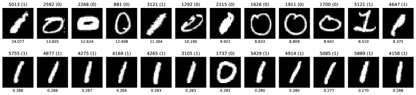
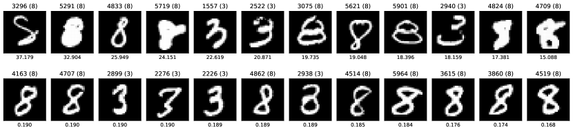
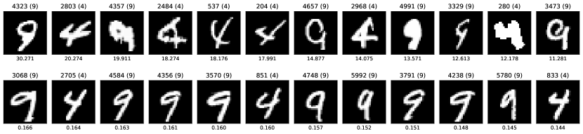
Figure 2: Digits ordered by diversity weight (index above with label in brackets, weight below). First two rows: pair 0-1, two middle rows: pair 3-8, last two rows: pair 4-9. Odd rows: twelve highest weighted, even row: twelve lowest weighted.

Results

An overview of our quantitative results in given in fig. 3. For three pairs of digits, we compare our diversity weights (DivW) method with three different loss term balances ($\gamma$) against a standard GAN. The balance of loss terms determines the emphasis on a uniform distribution of weights (lower $\gamma$) over higher diversity (higher $\gamma$). Accordingly, in the diversity weight optimisation, a balance of $\gamma=1.0$ corresponds to a full emphasis on diversity and no entropy loss, while $\gamma=0.5$ strikes an equal balance between the two.

Our results agree on almost all measures across all three digit pairs, except on IS which we discuss further below. As expected, the higher the emphasis on the diversity loss, the higher (and better) the VS (fig. 3, top left). This comes with a trade-off in sample fidelity and mode coverage, as quantified by PR (fig. 3, middle and bottom left) and FID (fig. 3, top right). However, when accounting for a weighted training dataset with our Weighted FID measure, the distance of our DivW model distribution to the target distribution is notably lower than or at least on par with the standard model (fig. 3, middle right).

Results on IS (fig. 3, bottom right) show the difficulty in distinguishing different pairs of digits. For the pairing 0-1, the standard model and the DivW $\gamma=0.6$ model score notably higher than the other two DivW models ($\gamma=0.8$ and $\gamma=1.0$), while their scores are lower for the pairings 3-8 and 4-9. This suggests that, even for the standard model it is difficult to model two similar digits like 3-8 and 4-9.

For visual inspection and qualitative analysis, we provide random samples in fig. 4 for all digit pairs and models.

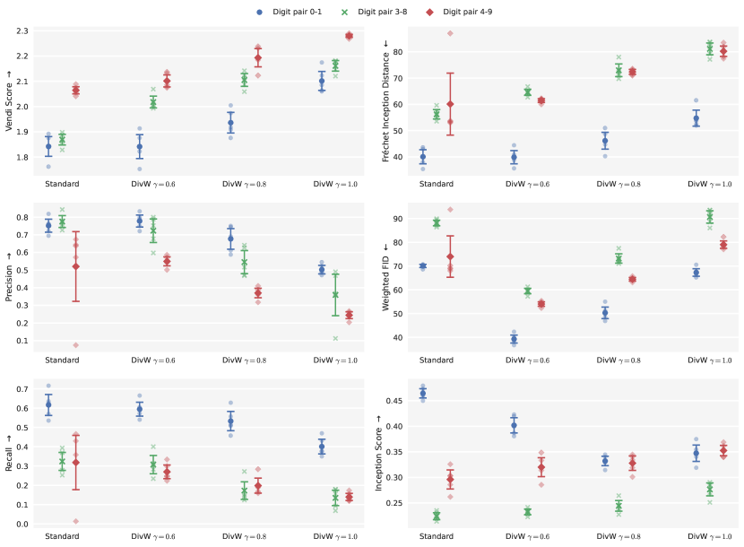
Figure 3: Performance comparison of our method (DivW) with different loss term balances ($\gamma$) against a standard GAN, trained on three digit pair datasets (blue circles: 0-1, green crosses: 3-8, red diamonds: 4-9) with six measures: VS, PR and IS (higher is better), as well as standard FID and weighted FID scores (lower is better). Means and 95% confidence intervals over five random seeds. Individual datapoints show means over five random sampling repetitions. The hyperparameter $\gamma$ provides control over the trade-off between diversity and typicality.

	Standard	DivW $\gamma=0.6$	DivW $\gamma=0.8$	DivW $\gamma=1.0$
Digits 0-1
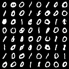
Digits 3-8
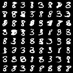
Digits 4-9

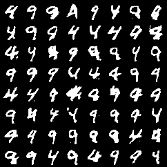
Figure 4: Random samples for all digit pairs (top row: 0-1, middle: 3-8, bottom: 4-9) from the standard models (left column) and our DivW models with different loss balances ($\gamma$). The hyperparameter $\gamma$ provides control over the trade-off between diversity and typicality.

Discussion

In recent years, research communities have become better aware of data biases and their impact on society through the proliferation of data-driven technologies. Likewise, CC researchers have highlighted its potential implications for CC research and the importance of mitigation (Smith, 2017; Loughran, 2022). Real-world datasets are limited sample from a complex world and should not be considered as the ‘ground truth’, or as representing the ‘true’ distribution. This practical impossibility further motivates our proposal to shift away from the predominant mode coverage paradigm.

Ongoing debates have not yet resulted in a uniformly accepted way of dealing with data bias in generative machine learning more generally, and CC specifically. One way to address data bias is to gather more or better data. But this is not always possible or practical, since collecting, curating and pre-processing new data is notoriously laborious, costly, or subject to limited access. Another way is to instead adjust the methodology of learning from data, such that a known data bias is mitigated. In this work, we focus on the latter and propose the diversity-weighted sampling scheme to address the imbalance of representation between majority and minority features in a dataset.

Diversity weights address the specific bias of data imbalance, particularly in unsupervised learning. In contrast to supervised settings, where class labels provide a clear categorisation of training examples, here common features are often shared between various types of examples. This makes it difficult to find an appropriate balance of training examples. Diversity weights give an indication of which type of examples are under-represented from a diversity-maximisation perspective. We draw a connection to issues of DEI as data biases often negatively affect under-represented groups (Bolukbasi et al., 2016; Zhao et al., 2017; Hendricks et al., 2018; Stock and Cisse, 2018).

Combining image generation models with multi-modal embedding models, like CLIP, enables complex text-to-image generative systems which can be doubly affected by data bias through the use of two data-driven models: the image generator and the image-text embedding. The discussion on embedding models, and other methods that can guide the search for artefacts, is beyond the scope of this paper. Our work focuses on the image generators powering these technologies. Yet, a conscious shift to mode balancing, in particular for the training of the underlying generative model, could support the mitigation of bias in text-to-image generation models, complementing existing efforts in prompt engineering after training (Colton, 2022).

It is worth noting, that our method also introduces bias, particularly emphasising under-represented features in the dataset. We do this explicitly and for a specific purpose. Other applications might differ in their perspective and objective and deem none or other biases less or more important. As we mentioned above, since a dataset cannot maintain its status of ‘ground truth’, the responsibility of reviewing and potentially mitigating data biases falls onto researchers and practitioners. We hope our work proves helpful in this task.

Related Work

Previous work primarily focuses on samples from minority groups and related data biases. Objectives range from mitigating such biases to improving minority coverage, i.e. achieving better image fidelity for underrepresented data examples. Some approaches employ importance weighting where weights are derived from density ratios, either via an approximation based on the discriminator’s prediction (Lee et al., 2021) or via an additional probabilistic classifier (Grover et al., 2019). Others propose an implicit maximum likelihood estimation framework to improve the overall mode coverage (Yu et al., 2020). These methods either depend on additional adversarily trained models or on more specific hybrid models. Our approach, instead, has two major benefits over previous work. First, it is model-agnostic and thus potentially applicable to a wide range of network architectures and training schemes. Second, it only adds an offline pre-computation step prior to conventional training procedures and during training solely intervenes at the data sampling stage.

Authors of previous work further argue for increased diversity, but do not evaluate on explicit measures of diversity. Results are reported on the standard metrics IS, as well as FID and PR which rely on the training dataset for reference. Consequently, they can only estimate sample fidelity and mode coverage as present in the data. We, instead, evaluate on measures designed to objectively quantify diversity.

Most importantly, while we argue for an adaptation of modelling techniques to allow for mode balancing to achieve higher output diversity, all related works operate under the mode coverage paradigm. In fact, Lee et al. (2021) include a discriminator rejection sampling step (Azadi et al., 2018) after training to undo the bias introduced by their importance sampling scheme.

Conclusions

We introduced a method to derive a weight vector over the examples in a training dataset, which indicate their individual contribution to the dataset’s overall diversity. Diversity weights allow to train a generative model with importance sampling such that the model’s output diversity increases.

Our work is motivated by potential benefits for computational creativity applications which aim to produce a wide range of diverse output for further design iterations, ranging from artistic over constrained to scientific creativity. We also highlight a connection to issues of data bias in generative machine learning, in particular data imbalances and the under-representation of minority features. The impracticality of easily mitigating data imbalances in an unsupervised setting further motivates our work.

In a proof-of-concept study, we demonstrated that our method increases model output diversity when compared to a standard GAN. The results highlight a trade-off between artefact typicality, i.e. the extent to which an artefact is a typical training, and diversity. Our method provides control over this trade-off via a loss balance hyperparameter.

Future Work

We plan to build on the present work in several ways. First, by refining our method, in particular the training procedure, to improve overall sample fidelity. For this, a thorough analysis and systematic comparison to related work is needed. The loss balance hyperparameter could further be tuned automatically by including it as a learnable parameter in the optimisation procedure. Apart from our gradient descent approach, there might be alternative exact or approximate methods for the diversity weight optimisation, e.g. constraint optimisation or analytical solutions.

Second, we plan to extend experimentation to other generative models and on bigger and more complex datasets to demonstrate the scalability of our approach. Since our method is architecture-agnostic, there remain many opportunities for future work to understand the effect and potential benefits of our method in other modelling techniques. As GAN training is notoriously unstable and requires careful tuning, other modelling techniques might prove more appropriate. Results on datasets representing humans are needed to demonstrate the capability of our method to mitigate issues of DEI resulting from data imbalances.

Moreover, empirical studies will be necessary to investigate how the shift from mode coverage to mode balancing can support diversity in a large range of CC applications.

Appendix

The tables below outline the experiments’ training hyperparameters and network architectures, which do not include any pooling, batchnorm or dropout layers. He initialisation (Kaiming uniform) is used for convolutional layers (conventional and upsampling) and Glorot initialisation (Xavier uniform) for fully connected (FC) layers.

Table 2: Architecture of WGAN-GP generator network. Upsampling convolutional layers (ConvTranspose) have kernel size 4 $\times$ 4, stride 2, padding 1, dilation 1.

WGAN Generator
Layer	Output	Activation
Input $z$	64
Linear (FC)	2,048	ReLU
Reshape	4 $\times$ 4 $\times$ 128
ConvTranspose	8 $\times$ 8 $\times$ 64	ReLU
Cut	7 $\times$ 7 $\times$ 64
ConvTranspose	14 $\times$ 14 $\times$ 32	ReLU
ConvTranspose	28 $\times$ 28 $\times$ 1	Sigmoid

Table 3: Architecture of WGAN-GP critic network. Convolutional layers have kernel size 5 $\times$ 5, stride 2, padding 2.

WGAN Critic
Layer	Output	Activation
Input	28 $\times$ 28 $\times$ 1
Conv	14 $\times$ 14 $\times$ 32	LeakyReLU(0.2)
Conv	7 $\times$ 7 $\times$ 64	LeakyReLU(0.2)
Conv	4 $\times$ 4 $\times$ 128	LeakyReLU(0.2)
Reshape	2,048
Linear (FC)	1

Table 4: Training hyperparameters

Hyperparameter	Value
Num steps	6,000
Num critic steps	5
Batch size	6,000
GP weight	10.0
LR generator	0.0001
LR critic	0.0001
Adam $\beta_{1}$	0.5
Adam $\beta_{2}$	0.9

References

- Azadi et al. (2018) Azadi, S.; Olsson, C.; Darrell, T.; Goodfellow, I.; and Odena, A. 2018. Discriminator Rejection Sampling. In ICLR.
- Barratt and Sharma (2018) Barratt, S., and Sharma, R. 2018. A Note on the Inception Score. In Proceedings of the ICML Workshop on Theoretical Foundations and Applications of Deep Generative Models.
- Berns and Colton (2020) Berns, S., and Colton, S. 2020. Bridging Generative Deep Learning and Computational Creativity. In Proceedings of ICCC.
- Berns et al. (2021) Berns, S.; Broad, T.; Guckelsberger, C.; and Colton, S. 2021. Automating Generative Deep Learning for Artistic Purposes: Challenges and Opportunities. In Proceedings of ICCC.
- Boden (2004) Boden, M. A. 2004. The Creative Mind: Myths and Mechanisms. Routledge, second edition.
- Bolukbasi et al. (2016) Bolukbasi, T.; Chang, K.-W.; Zou, J. Y.; Saligrama, V.; and Kalai, A. T. 2016. Man is to Computer Programmer as Woman is to Homemaker? Debiasing Word Embeddings. In Advances in NeurIPS, volume 29.
- Bradner, Iorio, and Davis (2014) Bradner, E.; Iorio, F.; and Davis, M. 2014. Parameters Tell the Design Story: Ideation and Abstraction in Design Optimization. In Proceedings of the Symposium on Simulation for Architecture & Urban Design.
- Broad et al. (2021) Broad, T.; Berns, S.; Colton, S.; and Grierson, M. 2021. Active Divergence with Generative Deep Learning - A Survey and Taxonomy. In Proceedings of ICCC.
- Colton (2022) Colton, S. 2022. Towards Educating Artificial Neural Systems. In Proceedings of the International Workshop on Neuro-Symbolic Learning and Reasoning.
- Friedman and Dieng (2022) Friedman, D., and Dieng, A. B. 2022. The Vendi Score: A Diversity Evaluation Metric for Machine Learning. ArXiv:2210.02410v1.
- Grover et al. (2019) Grover, A.; Song, J.; Kapoor, A.; Tran, K.; Agarwal, A.; Horvitz, E. J.; and Ermon, S. 2019. Bias Correction of Learned Generative Models using Likelihood-Free Importance Weighting. In Advances in NeurIPS, volume 32.
- Gulrajani et al. (2017) Gulrajani, I.; Ahmed, F.; Arjovsky, M.; Dumoulin, V.; and Courville, A. C. 2017. Improved Training of Wasserstein GANs. In Guyon, I.; Luxburg, U. V.; Bengio, S.; Wallach, H.; Fergus, R.; Vishwanathan, S.; and Garnett, R., eds., Advances in NeurIPS, volume 30.
- Hendricks et al. (2018) Hendricks, L. A.; Burns, K.; Saenko, K.; Darrell, T.; and Rohrbach, A. 2018. Women also Snowboard: Overcoming Bias in Captioning Models. In Proceedings of ECCV.
- Heusel et al. (2017) Heusel, M.; Ramsauer, H.; Unterthiner, T.; Nessler, B.; and Hochreiter, S. 2017. GANs Trained by a Two Time-Scale Update Rule Converge to a Local Nash Equilibrium. In Advances in NeurIPS, volume 30.
- Kandpal, Wallace, and Raffel (2022) Kandpal, N.; Wallace, E.; and Raffel, C. 2022. Deduplicating Training Data Mitigates Privacy Risks in Language Models. In Proceedings of ICML.
- King, Butcher, and Zalewski (2017) King, T.; Butcher, S.; and Zalewski, L. 2017. Apocrita - High Performance Computing Cluster for Queen Mary University of London. DOI:10.5281/zenodo.438045.
- Kingma and Ba (2015) Kingma, D. P., and Ba, J. 2015. Adam: A Method for Stochastic Optimization. In ICLR.
- Ko et al. (2023) Ko, H.-K.; Park, G.; Jeon, H.; Jo, J.; Kim, J.; and Seo, J. 2023. Large-scale text-to-image generation models for visual artists’ creative works. In International Conference on Intelligent User Interfaces.
- Kolmogorov (1933) Kolmogorov, A. 1933. Grundbegriffe der Wahrscheinlichkeitsrechnung. Springer-Verlag.
- Kynkäänniemi et al. (2019) Kynkäänniemi, T.; Karras, T.; Laine, S.; Lehtinen, J.; and Aila, T. 2019. Improved Precision and Recall Metric for Assessing Generative Models. In Advances in NeurIPS.
- Kynkäänniemi et al. (2023) Kynkäänniemi, T.; Karras, T.; Aittala, M.; Aila, T.; and Lehtinen, J. 2023. The Role of ImageNet Classes in Fréchet Inception Distance. In ICLR.
- Lee et al. (2021) Lee, J.; Hong, Y.; Kim, H.; and Chung, H. W. 2021. Self-Diagnosing GAN: Diagnosing Underrepresented Samples in Generative Adversarial Networks. In Advances in NeurIPS, volume 34.
- Liapis, Yannakakis, and Togelius (2014) Liapis, A.; Yannakakis, G. N.; and Togelius, J. 2014. Computational Game Creativity. In Proceedings of ICCC.
- Loughran and O’Neill (2017) Loughran, R., and O’Neill, M. 2017. Application Domains Considered in Computational Creativity. In Proceedings of ICCC.
- Loughran (2022) Loughran, R. 2022. Bias and Creativity. In Proceedings of ICCC.
- Madani et al. (2023) Madani, A.; Krause, B.; Greene, E. R.; Subramanian, S.; Mohr, B. P.; Holton, J. M.; Olmos, J. L.; Xiong, C.; Sun, Z. Z.; Socher, R.; Fraser, J. S.; and Naik, N. 2023. Large language models generate functional protein sequences across diverse families. Nature Biotechnology.
- Parmar, Zhang, and Zhu (2022) Parmar, G.; Zhang, R.; and Zhu, J.-Y. 2022. On Aliased Resizing and Surprising Subtleties in GAN Evaluation. In Proceedings of CVPR.
- Radford et al. (2021) Radford, A.; Kim, J. W.; Hallacy, C.; Ramesh, A.; Goh, G.; Agarwal, S.; Sastry, G.; Askell, A.; Mishkin, P.; Clark, J.; Krueger, G.; and Sutskever, I. 2021. Learning Transferable Visual Models From Natural Language Supervision. In Proceedings of ICML.
- Ramesh et al. (2021) Ramesh, A.; Pavlov, M.; Goh, G.; Gray, S.; Voss, C.; Radford, A.; Chen, M.; and Sutskever, I. 2021. Zero-Shot Text-to-Image Generation. In Proceedings of ICML.
- Razeghi et al. (2022) Razeghi, Y.; Logan IV, R. L.; Gardner, M.; and Singh, S. 2022. Impact of Pretraining Term Frequencies on Few-Shot Reasoning. ArXiv:2202.07206v2.
- Ritchie (2007) Ritchie, G. 2007. Some Empirical Criteria for Attributing Creativity to a Computer Program. Minds and Machines 17(1).
- Runco and Jaeger (2012) Runco, M. A., and Jaeger, G. J. 2012. The Standard Definition of Creativity. Creativity Research Journal 24(1).
- Saharia et al. (2022) Saharia, C.; Chan, W.; Saxena, S.; Li, L.; Whang, J.; Denton, E.; Ghasemipour, S. K. S.; Gontijo-Lopes, R.; Ayan, B. K.; Salimans, T.; Ho, J.; Fleet, D. J.; and Norouzi, M. 2022. Photorealistic Text-to-Image Diffusion Models with Deep Language Understanding. In Advances in NeurIPS, volume 35.
- Salimans et al. (2016) Salimans, T.; Goodfellow, I.; Zaremba, W.; Cheung, V.; Radford, A.; and Chen, X. 2016. Improved Techniques for Training GANs. In Advances in NeurIPS, volume 29.
- Smith (2017) Smith, G. 2017. Computational Creativity and Social Justice: Defining the Intellectual Landscape. In Proceedings of the Workshop on Computational Creativity and Social Justice at ICCC.
- Stanley and Lehman (2015) Stanley, K. O., and Lehman, J. 2015. Why Greatness Cannot Be Planned: The Myth of the Objective. Springer.
- Stock and Cisse (2018) Stock, P., and Cisse, M. 2018. ConvNets and ImageNet Beyond Accuracy: Understanding Mistakes and Uncovering Biases. In Proceedings of ECCV.
- Szegedy et al. (2016) Szegedy, C.; Vanhoucke, V.; Ioffe, S.; Shlens, J.; and Wojna, Z. 2016. Rethinking the Inception Architecture for Computer Vision. In Proceedings of CVPR.
- Veale, Cardoso, and Pérez y Pérez (2019) Veale, T.; Cardoso, F. A.; and Pérez y Pérez, R. 2019. Systematizing Creativity: A Computational View. Computational Creativity: The Philosophy and Engineering of Autonomously Creative Systems 1–19.
- Vimpari et al. (2023) Vimpari, V.; Kultima, A.; Hämäläinen, P.; and Guckelsberger, C. 2023. “An Adapt-or-Die Type of Situation”: Perception, Adoption, and Use of Text-To-Image-Generation AI by Game Industry Professionals. ArXiv:2302.12601v3.
- Volz et al. (2018) Volz, V.; Schrum, J.; Liu, J.; Lucas, S. M.; Smith, A.; and Risi, S. 2018. Evolving Mario Levels in the Latent Space of a Deep Convolutional Generative Adversarial Network. In Proceedings of GECCO.
- Yu et al. (2020) Yu, N.; Li, K.; Zhou, P.; Malik, J.; Davis, L.; and Fritz, M. 2020. Inclusive GAN: Improving Data and Minority Coverage in Generative Models. In Vedaldi, A.; Bischof, H.; Brox, T.; and Frahm, J.-M., eds., Proceedings of ECCV. Springer International Publishing.
- Zhao et al. (2017) Zhao, J.; Wang, T.; Yatskar, M.; Ordonez, V.; and Chang, K.-W. 2017. Men Also Like Shopping: Reducing Gender Bias Amplification using Corpus-level Constraints. In Proceedings of the Conference on Empirical Methods in Natural Language Processing.
- Zhong et al. (2019) Zhong, P.; Mo, Y.; Xiao, C.; Chen, P.; and Zheng, C. 2019. Rethinking Generative Mode Coverage: A Pointwise Guaranteed Approach. In Advances in NeurIPS, volume 32.
- CC
- computational creativity
- DL
- deep learning
- GM
- generative model
- ML
- machine learning
- GAN
- generative adversarial network
- VAE
- variational auto-encoder
- CLIP
- contrastive language-image pre-training
- DiaGAN
- Self-Diagnosing GAN
- InclGAN
- Inclusive GAN
- SAGAN
- Self-Attention Generative Adversarial Network
- SNGAN
- Spectral Normalisation GAN
- WGAN-GP
- Wasserstein GAN with gradient penalty
- LIGM
- large image generation model
- FID
- Fréchet Inception Distance
- wFID