Few-shot Class-incremental Pill Recognition

Abstract

The automatic pill recognition system is of great significance in improving the efficiency of the hospital, helping people with visual impairment, and avoiding cross-infection. However, most existing pill recognition systems based on deep learning can merely perform pill classification on the learned pill categories with sufficient training data. In practice, the expensive cost of data annotation and the continuously increasing categories of new pills make it meaningful to develop a few-shot class-incremental pill recognition system. In this paper, we develop the first few-shot class-incremental pill recognition system, which adopts decoupled learning strategy of representations and classifiers. In learning representations, we propose the novel Center-Triplet loss function, which can promote intra-class compactness and inter-class separability. In learning classifiers, we propose a specialized pseudo pill image construction strategy to train the Graph Attention Network to obtain the adaptation model. Moreover, we construct two new pill image datasets for few-shot class-incremental learning. The experimental results show that our framework outperforms the state-of-the-art methods.

I Introduction

Automatic prescription pill recognition is dedicated to performing the recognition task of oral pills dispensed according to a prescription. Unlike the problem of pill recognition in application scenarios such as pill factory [1] and pill retrieval system [2], the prescription pill recognition system usually needs to simultaneously recognize pills related to multiple classes and multiple instances contained in the prescription. Throughout the world, numerous pill misuse incidents are caused by various reasons every year. Developing an automatic prescription pill recognition system can well improve this phenomenon. The significance of this system can be broadly summarized as follows: first, it can release the dispensing staff from the intensive and laborious work; second, this system can double-check the dispensed pills to ensure they are consistent with the prescription; third, the system can provide technical supports for many application scenarios, such as assisting the proper use of medications for visually impaired people (e.g. the blind and the elderly), and reducing the risk of cross-infection in the treatment of highly infectious diseases.

There are some existing works [3, 4, 5, 6, 7, 8, 9, 10, 11, 12, 13, 14] focusing on the development of automatic pill recognition system. In the early stage, the pill recognition systems are mainly based on feature engineering [3, 4, 5]. For instance, the first pill recognition work [3] shows the effectiveness of the shape, color, size, and imprint features in the recognition process, and another work [5] focuses on the analysis of text imprint features on the pill surface. Since deep learning technology has shown overwhelming advantages in many computer vision tasks, it has recently dominated research on automatic pill recognition. The related studies can broadly be divided into one-stage frameworks [12, 13, 14] and two-stage frameworks [6, 7, 8, 9, 10]. One-stage frameworks usually employ the single pill recognition pipeline, which does not separate the localization process. For instance, the CenterNet is utilized to directly localize and classify the pill in the image in [13]. Besides, a comparison experiment to explore the effectiveness of different one-stage methods, including RetinaNet, SSD, and YOLO v3, is conducted in [12]. Unlike one-stage frameworks, two-stage frameworks generally need a pre-processing step for object localization, where the segmentation-based and detection-based methods are widely used. For instance, [8] uses the enhanced feature pyramid network to perform the localization, and [10] employs the fully convolutional network to segment the potential objects. After the localization, the second stage aims to classify potential objects.

Although the existing studies make some achievements, pill recognition remains an under-exploited field with the following challenges:

• The lack of realistic datasets. Existing pill datasets can be divided into single-object and multi-object datasets. For single-object datasets, such as the CURE dataset [11], each image contains only one pill, which differs from the practical multi-object application scenario. Although some works propose multi-object datasets [9, 8], the pills in their images are manually separated, which is wholly deviated from the actual application scenario (e.g., examples shown in Fig. 1(a)). Actually, in the multi-object pill recognition scenario, the phenomenon of pill adhesion often occurs (e.g., examples shown in Fig. 1(b)). The practical system is expected to be able to handle the recognition task related to randomly placed pills of multiple classes and instances in an image. The lack of realistic pill image datasets hinders the development and application of pill recognition approaches.

  

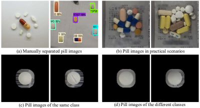
  Figure 1: The pill image examples of different datasets. (a) provides the pill images used in [8] and [9]. These pills are manually separated, which is against the practical scenario. (b) shows the images we collected from the real application scenario in hospitals, and it can be found that the phenomenon of pill adhesion often occurs. (c) and (d) show the single pills we extracted from the original images. (c) provides different sides of the same pill, and their different textures can lead to large intra-class variations. (d) demonstrates that the pills belong to different classes but have similar appearances, which can lead to small inter-class variations.

• Dynamic data stream and annotation cost. Currently, all the deep learning-based pill recognition frameworks are trained with the static data stream, which means they can only deal with the analysis of the learned task. However, the pill data are continuously updated with the evolution and invention of pills. Additionally, although deep learning methods make some progress, they still have the limitation of requiring plenty of labeled data for training. Whereas, the cost of data annotation is time-consuming and expensive. Furthermore, it is not practical to annotate large numbers of pill images of new classes. Unfortunately, the current deep learning-based pill recognition methods cannot well handle these bottlenecks.

• Large intra-class variations and small inter-class variations. Variations generated by different factors, such as random placement angle, illumination change, occlusion, and noise, result in significant effects on the pill appearance, causing large intra-class variations (e.g., examples shown in Fig. 1(c)). Besides, since only a few forms are available during the pill manufacturing process (as shown in Fig. 1(d), many pills of different classes are white and round), small inter-class variations are common in pill images.

To address the limitation of the high cost of data annotation, the first few-shot pill recognition framework is proposed in [11]. Unlike natural images, since pill images usually have symmetrical shapes, specific imprints, and certain colors, this system combines these features with triplet loss to perform the few-shot pill recognition task. Although the efforts made by [11] provide a solution for few-shot pill recognition, the other challenges mentioned above remain unaddressed to date. Therefore, in response to the challenges mentioned above, our paper proposes a new pill image dataset collected from the actual hospital scene and the first few-shot class-incremental framework for pill recognition. In summary, the main contributions of this paper are listed as follows:

• A new pill image dataset, namely FCPill, is proposed for the Few-shot Class-incremental Learning (FSCIL) task, where the images are sampled from eight groups of pill image data collected from seven hospitals in five Chinese cities. This dataset contains 144 base and 100 new classes. In addition, we sample another pill dataset, called miniCURE, from the public dataset CURE [11] in a similar way as miniImageNet to evaluate the effectiveness of our proposed method. miniCURE includes 91 base and 80 new classes.

• We propose the first few-shot class-incremental pill recognition framework, which adopts decoupled learning strategy of representations and classifiers. In representation learning, a novel Center-Triplet loss (CT loss) is proposed to perform discriminative representation learning. In classifier learning, a specialized pseudo pill image generation approach is proposed to train the Graph Attention Network (GAT) model for propagating the context between prototypes of base and new classes in the classifier.

• In the pre-processing part, we propose an improved U-Net, namely LCW-Net, to perform the localization of pill objects. It outperforms the related U-Net series in both segmentation performance and memory requirement. Besides, we reproduce mainstream FSCIL methods on the proposed FCPill dataset and miniCURE dataset to provide two new benchmarks for FSCIL algorithms.

The remainders of this paper are organized as follows: In Sec. II, we review the relevant basic knowledge and literature; Sec. III introduce the collection and construction of our proposed datasets; Sec. IV introduces our proposed methods in detail; Sec. V gives dataset details and experimental results; The conclusion is provided in Sec. VI.

II Related Work

II-A Few-shot Learning

The purpose of FSL is to design a machine learning algorithm that can rapidly generalize to new tasks containing only a few samples with supervised information based on previous knowledge [15, 16]. Each new task usually includes a support set and a query set, and the data in the two sets do not intersect [17]. The support set contains a few labeled training samples, which assist the algorithm based on prior knowledge to make predictions on the query set. The data in the support set is often described as $N-$way $K-$shot, which means that the support set contains $N$ classes, and each class has $K$ labeled samples. In recent years, plenty of works have focused on developing few-shot learning algorithms. They can broadly be summarized into optimization-based and metric learning-based methods [18]. Optimization-based methods train a model with data from previous base classes and then fine-tune the classifier or the whole model with data from the support set in the new task [19]. Our work is more relevant to metric learning-based methods, which generally learn feature representations through existing metric algorithms [19]. Metric learning-based methods concentrate on learning a robust backbone to generate high-quality and transferable feature representations [20]. The Siamese loss, which can minimize the distance between feature representations from the same class, and maximize otherwise, is used to perform the FSL task in [21]. The first few-shot pill recognition framework [11] adopts the Triplet loss, similar to the Siamese loss, to obtain discriminative feature representations to perform the FSL task.

II-B Class-incremental Learning

Class-incremental Learning (CIL) focuses on developing a machine learning algorithm that can continuously learn knowledge from a sequence of new classes while preserving the knowledge learned from previous classes [22, 23]. In the CIL setting, the data stream is usually in the form of a sequence of sessions, and each session has a training dataset and a testing dataset. These sessions usually consist of a base session and several incremental sessions. Different sessions have no overlapped classes. Once the learning process comes into the session $i$, the training datasets in previous sessions are unavailable. In contrast, the testing data used in the current session consists of the testing datasets from all previous and current sessions. The existing CIL algorithms can be roughly divided into three groups: parameter-based, distillation-based, and rehearsal-based methods [22]. Parameter-based methods [24, 25] try to assess the importance of each parameter in the original model and to avoid the crucial parameters from being changed. Knowledge distillation effectively transfers the knowledge of a base network to another. LwF [26] is the first approach to introduce knowledge distillation to incremental learning. Rehearsal-based methods [27, 28] save some previous instances for replaying when the model is trained for new classes to abstain from forgetting. iCaRL [29] is the first method that formally introduced CIL. It employs the decoupled approach for feature representation learning and classifier learning. iCaRL learns the nearest neighbor classifier with exemplars to realize the replay and combines distillation loss to alleviate catastrophic forgetting.

II-C Few-shot Class-incremental Learning

FSCIL is a recent machine learning topic proposed in [30]. Its purpose is to design a machine learning algorithm that can continuously learn knowledge from a sequence of new classes with only a few labeled training samples while preserving the knowledge learned from previous classes [30, 31]. In the FSCIL setting, the data stream usually consists of a base session with sufficient training data and a sequence of incremental sessions, whose training datasets are in the form of $N-$way $K-$shot. Once the learning process goes into session $i$, previous session training datasets are unavailable. In contrast, the testing data used in session $i$ consists of the testing datasets from all previous and current sessions. Recently, quite a few works have focused on developing the FSCIL algorithm. For instance, TOPIC [30] is the first algorithm specifically used to perform the FSCIL task. It uses the neural gas network to preserve the topology of features between the base and new classes to avoid forgetting [30]. The state-of-the-art CEC [32] adopts GAT to update the relationships between the base and new prototypes, which can help the classifier find better decision boundaries.

II-D Related Metric Loss

Triplet loss seeks to learn a backbone that can constrain the distance between feature representations of the same class less than the distance between feature representations of the different classes by a predefined margin value in the feature space. The illumination of Triplet loss is shown in Fig. 2(b). Specifically, for $\forall\left(x^{i}_{a},x^{i}_{p},x^{i}_{n}\right)\in\mathcal{T}$, the optimization purpose is

$$\|{f\left(x^{i}_{a}\right)-f\left(x^{i}_{p}\right)}\|+m<\|{f\left(x^{i}_{a}\right)-f\left(x^{i}_{n}\right)}\|$$ (1)

where $\mathcal{T}$ denotes the set of all the possible triplets of training samples. Each triplet of training samples consists of an anchor sample $x^{i}_{a}$, a positive sample $x^{i}_{p}$ with the same label as $x^{i}_{a}$, and a negative sample $x^{i}_{n}$ from another class. $m$ is the margin value. $f\left(\cdot\right)$ represents the feature representation output from the backbone. $\|\cdot\|$ denotes the calculation of Euclidean distance. Based on the optimization purpose in Eq. 1, the Triplet loss can be formulated as follows:

$$L_{t}=\sum^{N}_{i=1}\max(0,m+\|f\left(x^{i}_{a}\right)-f\left(x^{i}_{p}\right)\|$$ (2)

$$-\|f\left(x^{i}_{a}\right)-f\left(x^{i}_{n}\right)\|)$$

where $N$ denotes the triplet number in the mini-batch. When the triplets satisfy Eq. 1, the Triplet loss value will be zero. Otherwise, the Triplet loss will be calculated by the non-zero part of Eq. 2. Although the Triplet loss can ideally help the model learn discriminative feature representations, it faces some challenges in practice. For instance, the number of triplets for a large dataset is numerous, which usually contributes to slow convergence [33]. Meanwhile, not all the triplets can make progress in the training process. The performance highly depends on the mining of effective triplets [33].

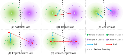
Figure 2: The illustration of the distributions of deep features learned by different losses. (a) Softmax loss aims to learn the decision boundary; (b) Triplet loss seeks to constrain the distance between features of the same class to be less than the distance between different classes by a predefined margin; (c) Center loss encourages the intra-class compactness; (d) Triplet-Center loss introduces Center loss into Triplet loss to encourage the intra-class compactness and inter-class separability; (e) Our proposed Center-Triplet loss further promote the intra-class compactness and inter-class separability by directly considering the distance between different class centers.

Center loss [34] is proposed to deal with the limitation of Softmax loss by encouraging the intra-class compactness in the face recognition task. It can reduce the intra-variance by learning a center for each class and pulling the feature representations in the current class close to its center in the feature space [35]. The illumination can be found in Fig.2(b). The definition of Center loss can be formulated as follows:

$$L_{c}=\sum^{N}_{i=1}\|f\left(x^{i}\right),c_{y_{i}}\|$$ (3)

where $f\left(x^{i}\right)$ is the representation of sample $x^{i}$, and $c_{y_{i}}$ is the corresponding class center of $x^{i}$. In the training process, the Center loss is skilled in promoting intra-class compactness. Nevertheless, the learned centers are usually unstable because their update is based on a mini-batch rather than the entire dataset in each iteration. Consequently, the Center loss has to be used under the joint supervision of Softmax loss in the training process.

Triplet-Center loss (TC loss) [33] is proposed to perform the multi-view 3D object retrieval. Since the Center loss [34] only considers the intra-class compactness and cannot deal with the problem of small overlaps between different classes, the TC loss is proposed to tackle this limitation by introducing Center loss into Triplet loss. Fig. 2(d) provides an illumination of TC loss. Concretely, the definition of TC loss is formulated as follows:

$$L_{tc}=\sum^{N}_{i=1}\max(0,m+\|f\left(x^{i}\right)-c_{y_{i}}\|$$ (4)

$$-\min_{j\neq y_{i}}\|f\left(x^{i}\right)-c_{j}\|)$$

where $c_{j}$ represents the learned class center that is different from $c_{y_{i}}$. TC loss can train the backbone to learn a corresponding center for each class and promote the distances between samples and centers from the same class to a predefined margin value less than those from different classes [33]. It promotes not only intra-class compactness but also strengthens inter-class separability.

III Dataset

III-A FCPill Dataset

III-A1 Original Data Collection

Existing pill datasets can be divided into single-object datasets and multi-object datasets where pills are manually separated, which is inconsistent with real application scenarios. In many hospital wards, patients are usually given pills in packets according to the prescription. The pills in a packet usually involve multiple classes and multiple instances, which are often adhered to or overlapped with each other. However, none of the existing datasets can reflect the real pill packet scenario. Therefore, to solve this drawback, we collect a large number of original pill packet images and their corresponding electronic prescription files from real hospital scenarios. Specifically, after obtaining the approval of the relevant ethics committee, we employ a device with a top camera and a bottom camera to take images of the pill packets. The top and bottom cameras take each pill packet’s colorful frontal image and the corresponding back image. Finally, we collected 473148 original pill packet images from seven hospitals in five cities in China.

III-A2 Pill Segmentation and Localization

In addition to the pill object, the original image generally contains a lot of noise, such as the contents of the prescription, patient name, and ward information. The noise could even deteriorate the learning of the pill recognition model. Besides, the pill packet image usually involves multiple pill objects. Therefore, to enable our proposed few-shot class-incremental pill recognition framework, we first need to segment and locate the pill objects from the complex background and then combine the segmentation results with their corresponding digital prescription file to create the single-pill dataset divided by category. In the segmentation process, we propose a novel network based on LCU-Net [36] and $W^{2}$-Net [11] to segment the pills, which is called LCW-Net. The detailed structure can be found in the supplemental material. LCW-Net adopts two U-shape structures similar to $W^{2}$-Net to obtain better segmentation results. However, since the number of parameters usually increases with the deepening of network layers, LCW-Net optimizes the parameter amount by reducing the feature map channel generated by hidden layers. Additionally, due to the different shapes and sizes of pills, LCW-Net employs the design of multiple receptive fields in LCU-Net to improve the adaptation ability. In the training process of the proposed LCW-Net, we utilize the back packet image after the dilation and erosion processing as the ground truth. As aforementioned, the phenomenon of pill adhesion often occurs. Thus, to address this problem, we are inspired by the segmentation of cell cluster [37] and combine the prediction scores generated by LCW-Net with the watershed algorithm to realize the segmentation of adhesion pills. As Tab. I shows, our proposed LCW-Net achieves the best segmentation results and reduces the memory cost by nearly 20 times compared to U-Net.

TABLE I: The performance of different segmentation networks. Our LCW-Net achieves the best segmentation results and reduces the memory cost by nearly 20 times compared to U-Net.

	U-Net	LCU-Net	$W^{2}$-Net	LCW-Net (Ours)
Dice	95.29%	95.24%	95.03%	95.30%
IoU	92.05%	92.00%	91.61%	92.10%
Memory	372.6 MB	108.6 MB	27.0 MB	19.1 MB

III-A3 Dataset Statistics

After the segmentation process, to create the dataset that fits the FSCIL setting, we filter the pill classes with more than 40 samples per class from the processed data, resulting in a dataset containing 244 classes. Each class in this dataset includes 20 training images and 20 testing images. Similar to the splits of CIFAR100, miniImageNet, and CUB200 in [30], the 244 classes are divided into 144 base classes and 100 new classes. The 100 new classes are further divided into ten incremental sessions, and the training data in each session is in the form of 10-way 5-shot.

III-B miniCURE Dataset

In addition to our proposed FCPill dataset, we evaluate our framework on CURE [11], a public pill image dataset originally proposed for few-shot learning. CURE contains 1873 images of 196 classes, and each class has approximately 45 samples. To make it fit the setting of FSCIL, we follow the similar splits as miniImageNet in [30] to sample 171 classes to create the miniCURE dataset, where 171 classes are divided into 91 base classes and 80 new classes. These new classes are further divided into eight incremental sessions, and the training data in each session is in the form of 10-way 5-shot.

IV Proposed Methodology

In this section, the problem setting of FSCIL is first introduced. Then, the motivations of our proposed method are described. Third, we provide an overview of our proposed framework. Finally, the details of the internal operations, including backbone learning, adaptation module training, and incremental classifier learning, are presented in detail.

IV-A Problem Setting

Assume $\{D^{0}_{train},D^{1}_{train},\cdots,D^{n}_{train}\}$ and $\{D^{0}_{test},D^{1}_{test},\cdots,D^{n}_{test}\}$ denote the training and testing datasets in FSCIL sessions. The $n$ means the incremental session number in the current FSCIL task. $D^{0}_{train}$ denotes the training dataset in the base session, which contains abundant labeled training data. $\forall$ integer $i\in[1,n],D^{i}_{train}$ is in form of $N-$way $K-$shot, which means the training dataset in session $i$ contains $N$ classes and each class has $K$ labeled samples. $D^{i}_{test}$ denotes the testing dataset in session $i$. $\forall$ integer $i\in[0,n]$, $L^{i}$ denotes the corresponding label space of $D^{i}_{train}$ and $D^{i}_{test}$. The relevant classes in different sessions have no intersection, i.e., $\forall$ integer $i,j\in[0,n]$ and $i\not=j$, $L^{i}{\cap}L^{j}=\emptyset$. When the training process comes into session $i$, only the entire $D^{i}_{train}$ is available, while the entire training datasets of previous sessions are no longer available. For the evaluation at session $i$, the testing data consists of all the testing datasets from current and previous sessions, i.e., $D^{0}_{test}\cup D^{1}_{test}\cup\cdots\cup D^{i}_{test}$.

IV-B Overall Framework

The details of our framework are provided in Fig. 3. Similar to the existing FSCIL methods [32, 18], our framework adopts the decoupled learning strategy of representations and classifiers to abstain from catastrophic forgetting and overfitting problems. Specifically, the backbone trained by base classes is fixed as a feature extractor to learn representations for both base and new classes. Only the classifiers are updated for new classes. Our framework can be divided into three stages.

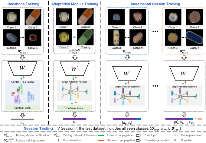
Figure 3: The framework of few-shot class-incremental pill recognition. To avoid the problems of overfitting and catastrophic forgetting, the framework adapts the decoupled learning of representations and classifiers. The training process consists of three stages: a) in the base session training stage, the proposed CT loss is used to learn discriminative feature representations since many pills from different classes have similar characteristics; b) in the pseudo incremental training stage, a specialized pseudo pill image generation approach is proposed to simulate the real incremental scenario to train the GAT adaptation module so that it can propagate contextual information between base and novel classes; c) in the incremental session training stage, the fixed backbone is used to generate original novel prototypes by averaging extracted features, and the GAT adaptation module learned in the pseudo incremental training stage is applied to update base and novel prototypes to generate the final classifiers.

Base session training for learning discriminative features. Since the main challenges of the FSCIL task are the catastrophic forgetting of previous knowledge and the overfitting of new classes with a few labeled samples. We adopt the decoupled learning strategy of representations and classifiers. Specifically, in this stage, we aim to learn a robust backbone with the base training data, which is fixed as a feature extractor to generate representations for both base and novel classes. Since pill images face the challenge of large intra-class and small inter-class variations, distinguishing them is more complicated than natural images. However, many existing FSCIL methods utilize the traditional Softmax loss to train the backbone, such as CEC [32]. The feature representations learned by Softmax loss are not sufficiently discriminative since its purpose is to find a decision boundary between different classes [33]. Nevertheless, among many FSL methods [11, 38, 39], Triplet loss is widely used to learn discriminative feature representations, which can make the distance between representations from the same class some margin value smaller than the distance between representations from the different classes. Thus, we want to import the Triplet loss into FSCIL. Although the Triplet loss can make the distances between the same class smaller than between different classes, it cannot consider the inter-distance within one class [33]. Moreover, triplet mining also has a significant impact on the training process. Easy or too-hard triplets negatively impact the training process [40]. To break through these bottlenecks, we propose a novel Center-Triplet (CT) loss to perform the representation learning. It performs the discriminative representation learning by selecting an anchor class and constraining the distance between the sample in this class and its center to be a predefined margin value less than the distance between this anchor center and the nearest center of another class. The details of CT loss are described in Sec. IV-C.

Pseudo incremental session training for learning GAT adaptation module. Traditional supervised deep learning aims to find the discriminative decision boundaries between learned classes. Adding new classes directly can invalidate the decision boundaries of the previous model to some extent, which may hinder the classification performance. Consequently, to update the decision boundaries between different classes, we employ the GAT used in CEC [32] to learn an adaptation module to propagate the context information between prototypes of base and novel classes. Since training GAT in the incremental learning scenario is necessary to acquire the adaptation model, our framework proposes the pseudo incremental learning stage. Concretely, we propose a random color and text transform algorithm inspired by the characteristics between pills of different classes to create pseudo pill classes. These pseudo pill images are combined with the sampling base classes to train the GAT adaptation module. Specifically, our pre-trained backbone will learn the discriminative feature representations for both the base and pseudo classes, and these representations will be seen as the nodes in the graph. Then, the GAT adaptation module based on the attention mechanism is applied to learn the relationships between different nodes and update these nodes. The Softmax loss is used in the GAT adaptation module training process. The details of pseudo incremental learning are described in Sec. IV-D.

Incremental session training. In the third incremental session training stage, the feature extractor trained by CT loss is employed to extract the feature representations for the images from incremental sessions. These feature representations will be averaged to generate the prototypes for their corresponding classes. Finally, the GAT adaptation module trained in the second stage is used to obtain the final classifiers by propagating the context information between the base and new prototypes.

IV-C Backbone Training using Center-Triplet Loss

Since Triplet loss can assist deep learning models in learning discriminative feature representations, we want to use it to train an efficient backbone. However, Triplet loss has some bottlenecks in the network optimization process. As we mentioned in Sec. II-D, not all the triplets in $\mathcal{T}$ can promote model optimization. Quite a few potential triplets are neglected. Generally, the majority of triplets in $\mathcal{T}$ belong to the easy triplets that satisfy Eq. 1, and they cannot contribute to the training process. Only semi-hard and hard triplets in $\mathcal{T}$ can make progress for the model optimization. The definitions of semi-hard and hard triplets are formulated as:

$$\|h_{f\left(x^{i}_{a}\right),f\left(x^{i}_{p}\right)}\|<\|h_{f\left(x^{i}_{a}\right),f\left(x^{i}_{n}\right)}\|<\|h_{f\left(x^{i}_{a}\right),f\left(x^{i}_{p}\right)}\|+m$$ (5)

$$\|h_{f\left(x^{i}_{a}\right),f\left(x^{i}_{n}\right)}\|<\|h_{f\left(x^{i}_{a}\right),f\left(x^{i}_{p}\right)}\|$$ (6)

where $h_{f\left(x^{i}_{a}\right),f\left(x^{i}_{p}\right)}$ and $h_{f\left(x^{i}_{a}\right),f\left(x^{i}_{n}\right)}$ represent $f\left(x^{i}_{a}\right)-f\left(x^{i}_{p}\right)$ and $f\left(x^{i}_{a}\right)-f\left(x^{i}_{n}\right)$ for short. Although semi-hard and hard triplets can converge the deep learning model in theory, too-hard triplets, in which the negative sample is extremely close to the anchor sample in the feature space, can lead to terrible local minima early in the training process. It can result in a collapsed model [41]. Specifically, for triplet $t:=\left(x^{i}_{a},x^{i}_{p},x^{i}_{n}\right)$, the gradient with respect to the feature representation of hard sample $f(x^{i}_{n})$ can be formulated by:

$$\partial_{f(x^{i}_{n})}L_{t}=\frac{h_{f\left(x^{i}_{a}\right),f\left(x^{i}_{n}\right)}}{\|h_{f\left(x^{i}_{a}\right),f\left(x^{i}_{n}\right)}\|}w(t)$$ (7)

where $w(\cdot)$ denotes some function that is one part of the partial derivative. Form Eq. 7, it can be found that the first term can determine the direction of the gradient [40]. When the triplet is too-hard, $\|h_{x^{i}_{a},x^{i}_{n}}\|$ will have a small value. If the feature representations estimated by the training model contain enough noise, Eq. 7 will be formed as:

$$\partial_{f(x^{i}_{n})}L_{t}=\frac{h_{f\left(x^{i}_{a}\right),f\left(x^{i}_{n}\right)}+z}{\|h_{f\left(x^{i}_{a}\right),f\left(x^{i}_{n}\right)}+z\|}w(t)$$ (8)

where $z$ stands for the noise. The direction of the gradient will be significantly affected by noise $z$. It means that the gradient of the too-hard triplet can easily fall into the saddle point during the back-propagation. Since the hard triplet easily leads to unstable gradients, semi-hard triplet mining is commonly used [41, 42]. Although semi-hard triplets can help the backbone converge rapidly at first, at some point, with no semi-hard triplets left in the band, the model optimization process will be hindered [40]. This situation is also reported in the FaceNet training process [41]. Consequently, it can be found that how to mine triplets greatly impacts the training process.

In addition to the problem of triplet mining, the triplet definitions make some potential easy triplets be ignored. Concretely, assuming the margin value $m$ in Triplet loss satisfies $m<\left|b-a\right|$, where $t_{1}:=\left(A_{1},A_{2},B_{1}\right)$ is the triplet shown in Fig. 4(a), $a=\|f\left(A_{1}\right)-f\left(A_{2}\right)\|$, and $b=\|f\left(A_{1}\right)-f\left(B_{1}\right)\|$. According to the definition, both triplet $t_{1}$ and $t_{2}:=\left(A_{3},A_{4},B_{2}\right)$ belong to easy triplets. According to Fig. 4(b), both the intra-class and inter-class distances in triplet $t_{2}$ are $n$ longer than those in triplet $t_{1}$. It means that no matter how large the $n$ is, triplet $t_{2}$ always satisfies the definition of easy triplet and is disabled to promote intra-class compactness. Although the time-consuming mining of semi-hard or hard triplets can contribute to the model optimization, the potential easy triplets containing abundant intra-class distance information are directly ignored. Thus, we hope all the potential triplets in $\mathcal{T}$ can contribute to the training process. The large intra-class distances existing in some easy triplets prompt us to pay more attention to take full advantage of them to encourage intra-class compactness further.

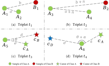
Figure 4: The examples of different triplets. (a) and (b) are triplets used in Triplet loss. (c) and (d) are triplets used in Triplet-Center loss. Assuming that (a) is an easy triplet, no matter what the value of $n$ in (b) is, (b) satisfies the definition of easy sample; Similarly, assuming that (c) is an easy triplet, no matter what the value of $\alpha$ in (d) is, (d) satisfies the definition of the easy sample. It can be found that some potential triplets are ignored.

Although TC loss can promote intra-class compactness by introducing the mechanism of Center loss into Triplet loss, it still has some limitations. The triplet $\left(x^{i},c_{y_{i}},c_{j}\right)$ used in TC loss consists of a sample $x^{i}$, its corresponding class center $c_{y_{i}}$, and the hardest negative class center $c_{j}$ (i.e. the nearest center of the another classes, $y_{i}\neq j$). For triplet $\left(x^{i},c_{y_{i}},c_{j}\right)$, the gradient with respect to the learned negative center $c_{j}$ can be formulated by:

$$\partial_{c_{j}}L_{tc}=\frac{h_{f\left(x^{i}\right),c_{j}}}{\|h_{f\left(x^{i}\right),c_{j}}\|}w(t)$$ (9)

where $h_{f\left(x^{i}\right),c_{j}}$ stands for $f\left(x^{i}\right)-c_{j}$. Since the TC loss always mines the nearest negative center for the sample $x_{i}$, the value of distance $\|h_{f\left(x^{i}\right),c_{j}}\|$ may be small in some cases. Similar to Triplet loss, if the feature representation predicted by the training model contains enough noise, the Eq. 9 will be formulated by:

$$\partial_{c_{j}}L_{tc}=\frac{h_{f\left(x^{i}\right),c_{j}}+z}{\|h_{f\left(x^{i}\right),c_{j}}+z\|}w(t)$$ (10)

The noise $z$ will dominate the gradient direction, and the optimization process will be unstable. Besides, TC loss only considers the relative relationship between $\|f\left(x^{i}\right)-c_{y_{i}}\|$ and $\|f\left(x^{i}\right)-c_{j}\|$. This limitation makes TC loss ignores the distance relationship between center $c_{y_{i}}$ and $c_{j}$. Specifically, consuming $m<\left|d-e\right|$, where $d$ and $e$ are the distance values shown shown in Fig. 4. According to Eq. 4, both triplet $t_{3}:=\left(A_{5},c_{A},c_{B}\right)$ and $t_{4}:=\left(A_{6},c_{A},c_{D}\right)$ in Fig. 4 cannot contribute to the model training process. Nevertheless, the distance between $c_{A}$ and $c_{B}$ in $t_{3}$ is significantly smaller than that in $t_{4}$. We hope that feature representations of different classes can be separated as much as possible in the feature space, which puts forward high requirements for intra-class compactness and the degree of separation between their centers.

To address the bottlenecks of Triplet loss and TC loss, we propose a novel metric loss function named CT loss. It concentrates on learning an efficient backbone by simultaneously strengthening the intra-class compactness and inter-class separability in the feature space. The triplet format used in CT loss is the same as in TC loss, which consists of a single sample $x_{i}$, its corresponding class center $c_{y_{i}}$, and another nearest class center $c_{j}$. Those triplets in each mini-batch are used to compute the value of CT loss. Concretely, for each effective triplet $\left(x^{i},c_{y_{i}},c_{j}\right)$ in the mini-batch, CT loss seeks to update the backbone so that it can constrain the distance between the feature representation of $x_{i}$ and its corresponding class center $c_{y_{i}}$, $i.e.$ the value of $\|f\left(x^{i}\right)-c_{y_{i}}\|$, less than the distance between $c_{y_{i}}$ and another nearest class center $c_{j}$, $i.e.$ the value of $\|c_{y_{i}}-c_{j}\|$, by a predefined margin value $m$. The illumination of CT loss is provided in Fig. 2(e). Mathematically, the definition of CT loss can be formulated as follows:

$$L_{ct}=\sum^{N}_{i=1}\max(0,m+\|f\left(x^{i}\right)-c_{y_{i}}\|$$ (11)

$$-\min_{j\neq y_{i}}\|c_{y_{i}}-c_{j}\|)$$

In the training process, we adopt the joint supervision based on both Softmax loss and our proposed CT loss because the class centers used in CT loss are randomly initialized and updated based on the mini-batches rather than the entire dataset. The Softmax loss can help to find better class centers. Therefore, we combine Softmax loss and CT loss to train the backbone, which can be formulated as follows:

$$L_{total}=L_{sm}+\lambda L_{ct}$$ (12)

where $L_{sm}$ denotes the Softmax loss, and $\lambda$ is a hyper-parameter used to balance the CT loss and Softmax loss.

Compared with Triplet loss, the proposed CT loss can take full advantage of the intra-class distances between samples and their corresponding class centers to encourage intra-class compactness since it adopts the same triplet format as TC loss and the intra-class distance constraining strategy based on Center loss. Furthermore, CT loss has a more vital anti-noise ability in the process of gradient back-propagation than TC loss since the negative pair of triplet in our method is composed of two different class centers, which generally contain less noise than the estimated feature representations. Besides, compared with Triplet loss, CT loss directly considers the distance between different class centers rather than between a sample and another class center. This difference makes CT loss have better inter-class separability than TC loss. Benefiting from these advantages, CT loss has excellent potential in the few-shot class-incremental pill recognition task.

IV-D Adaptation Module Training under Pseudo Incremental Scenario

The conventional supervised deep learning method aims to learn an efficient classifier to determine the appropriate decision boundaries between the learned classes. Adding new classes directly may lead to the invalidation of existing decision boundaries. Therefore, to find the balance between old and new classes, our proposed framework utilizes a GAT-based adaptation module same as [32] to tackle this problem, which has great potential to obtain better decision boundaries between old and new classes due to its extensible topological structure and self-attention-based update mechanism. In detail, the prototypes of previous and new classes in the classifier can be seen as the nodes in a graph. GAT’s self-attention mechanism can propagate contextual information between these nodes in the graph and update them. To enable the GAT-based adaptation module to update the classifier in the real incremental scenario, we create the pseudo incremental learning stage to train it.

In the pseudo incremental learning stage, we focus on building pseudo incremental pill image data to simulate the real class-incremental learning scenario. The pseudo training data will be combined with the base training dataset $D^{0}_{train}$ to train the GAT-based adaptation module, enabling it to function in the real incremental scenario. Since the pill directions in the images are not fixed, the random rotation strategy with a large degree in CEC is eliminated in our pseudo pill image generation process. Instead, we carefully analyze the differences between different pills, and we find that these differences mainly relate to the color, the imprint text on the surface, etc. Consequently, to promote the pseudo image data to be more realistic, we propose a novel strategy specifically for building pseudo pill image data by randomly adding imprint text on the pill surface and changing the color distribution. The implementation details can be found in the pseudo code of our proposed pseudo incremental learning, which is shown in Alg. 1.

Input: Pre-trained backbone $W$, Random initial GAT model $\mathcal{G}_{init}$, and base training dataset $D^{0}_{train}$

Output: The well trained GAT model $\mathcal{G}_{trained}$

1 while not done do

2       $\{S_{b},Q_{b}\},\{S_{i},Q_{i}\}\leftarrow$ Sample data from $D^{0}_{train}$ to construct the support and query sets in pseudo base and incremental datasets

3       for class $c$ in $N$ do

4             $p,q\leftarrow$ Random select a flag value from $\{0,1\}$, and they are not equal to 0 simultaneously.

5             if $p==1$ then

6                   $\sigma\leftarrow$ Random select a value from $(0.5,1)$

7                   $\{S_{i},Q_{i}\}\leftarrow$ Use $\sigma$ to scale a random RGB channel in images from class $c$ of $\{S_{i},Q_{i}\}$

8             end if

9            if $q==1$ then

10                   $\eta\leftarrow$ Random select a value from $\{1,2,3\}$

11                   $\{S^{\prime}_{i},Q^{\prime}_{i}\}\leftarrow$ Overlay the pseudo imprint text on pill images from class $c$ of $\{S_{i},Q_{i}\}$, and $\eta$ controls its size.

12             end if

13            

14       end for

15      $\phi_{b},\phi_{i}\leftarrow$ Learn FC layer on $W$ with $S_{b}$ and $S^{\prime}_{i}$

16       $\{\phi^{\prime}_{b},\phi^{\prime}_{i}\}\leftarrow$ Update classifier $\{\phi_{b},\phi_{i}\}$ using $\mathcal{G}_{init}$

17       $y^{\prime}\leftarrow$ Make predictions for $\{Q_{b},Q^{\prime}_{i}\}$ based on $W$ and $\{\phi^{\prime}_{b},\phi^{\prime}_{i}\}$

18       The loss value $\leftarrow$ Calculate the Softmax loss $L_{sm}(y,y^{\prime})$

19       $\mathcal{G}_{trained}\leftarrow$ Optimize $\mathcal{G}_{init}$ with SGD

20 end while

Algorithm 1 Pseudo incremental learning. $N$ is the number of pseudo incremental classes; $y$ and $y^{i}$ represent the ground truth and predicted labels.

The proposed pseudo incremental learning is inspired by meta-learning, which aims to transfer the knowledge learned from previous tasks to perform the new task [32]. The proposed pseudo incremental learning strategy utilizes the base training dataset $D^{0}_{train}$ in our FSCIL task to create a sequence of pseudo incremental tasks to enable the learning of the GAT adaptation module. To make the GAT adaptation module can perform the real class-incremental pill recognition task, our pseudo incremental task is required to be close to the real scenario. Therefore, each pseudo incremental task includes the pseudo base and incremental classes. The pseudo base classes are directly sampled from $D^{0}_{train}$, and each class contains a support set $S_{b}$ and a query set $Q_{b}$. Differently, we create the pseudo incremental classes by randomly adding imprint text on the pill surface and or changing the color distribution of the sampled image data from the rest part in $D^{0}_{train}$. This approach can promote the pseudo incremental data close to the real incremental data. Like $(S_{b},Q_{b})$, each pseudo incremental class also consists of a support set and a query set. It can be formed as $(S^{\prime}_{i},Q^{\prime}_{i})$. After building the pseudo base and incremental classes, the backbone $W$ trained by CT loss is employed to learn the classifier $\phi_{b}$ and $\phi_{i}$ for $S_{b}$ and $S^{\prime}_{i}$, respectively. These classifiers are concatenated and fed into the initial GAT model $\mathcal{G}_{init}$ for updating. Then, the updated classifier $\{\phi^{\prime}_{b},\phi^{\prime}_{i}\}$ is combined with the backbone $W$ to make predictions for the query sets $\{Q_{b},Q^{\prime}_{i}\}$. After that, the Softmax loss is employed to calculate the loss value between the ground truth labels and prediction results to optimize the GAT adaptation module. Once the GAT adaptation module is learned, the parameters inside will be fixed to perform the real incremental tasks.

IV-E Incremental Classifier Learning

In the real class-incremental task, the classifier is required to continually adopt the new classes without forgetting the knowledge learned from previous classes. To achieve this goal, the backbone trained by CT loss is fixed, which can avoid catastrophic forgetting. Besides, the learning of classifiers significantly impacts the performance. The decision boundaries may be invalidated if the prototypes of new classes are directly concatenated with the previous classifier. Consequently, we utilize a GAT adaptation module $\mathcal{G}_{trained}$ trained by our proposed pseudo incremental learning approach to address this bottleneck.

Concretely, since the dataset used in our few-shot class-incremental pill recognition task consists of a base session and several incremental sessions, we denote the initial classifier learned on session $I$ as the matrix $\phi_{I}\in\mathbb{R}^{N_{I}\times C}$, where $N_{I}$ means the number of classes in session $I$ and $C$ denotes the number of feature channel. The classifier $\phi_{I}\in\mathbb{R}^{N_{I}\times C}$ can be formulated as:

$$\phi_{I}=\left\{\overrightarrow{\varphi}^{1}_{0},\overrightarrow{\varphi}^{2}_{0},\cdots,\overrightarrow{\varphi}^{c}_{i},\cdots\overrightarrow{\varphi}^{N_{I}}_{I}\right\}$$ (13)

where $\overrightarrow{\varphi}^{c}_{i}$ represents the prototype of class $c$ in session $i$. We utilize the pre-trained GAT adaptation module to update the prototypes to find the appropriate decision boundaries between old and new classes. The GAT adaptation module can model the classifier $\phi_{I}$ as the graph structure. The prototypes in $\phi_{I}$ can be seen as the notes in the graph. The GAT adaptation module can utilize the relationships between different notes and the self-attention mechanism to update them. To illustrate the updating process in detail, we take the node $\overrightarrow{\varphi}^{j}$ in the graph as an example. The attention coefficients between the node $\overrightarrow{\varphi}^{j}$ and all nodes in the graph are first calculated. The calculation process can be formulated as follows:

$$\forall\,\overrightarrow{\varphi}^{k}\in\phi_{I},e_{jk}=\left\langle\psi\left(\overrightarrow{\varphi}^{j}\right),\theta\left(\overrightarrow{\varphi}^{k}\right)\right\rangle$$ (14)

where $\psi$ and $\theta$ are the linear functions that can project the initial prototype $\overrightarrow{\varphi}^{j}$ and $\overrightarrow{\varphi}^{k}$ into a new metric space, and $\langle\cdot,\cdot\rangle$ denotes the similarity function that computes the inner product between two notes. After calculating all the attention coefficients, the Softmax function is applied to normalize them. The final attention coefficient $a_{jk}$ between note $\overrightarrow{\varphi}^{j}$ and $\overrightarrow{\varphi}^{k}$ is obtained by

$$a_{jk}={\rm Softmax}\left(e_{jk}\right)=\frac{{\rm exp}(e_{jk})}{\sum_{h=1}^{|\phi_{I}|}{\rm exp}(e_{jh})}$$ (15)

Based on all the normalized attention coefficients, the updating process of prototype $\overrightarrow{\varphi}^{j}$ can be formulated as follows:

$$\overrightarrow{\varphi}^{j\prime}=\overrightarrow{\varphi}^{j}+\sum_{k=1}^{|\phi_{I}|}\left(a_{jk}\boldsymbol{\rm U}\overrightarrow{\varphi}^{k}\right)$$ (16)

where $\boldsymbol{\rm U}$ represents the weight matrix of a linear transformation. The updating of all the prototypes in classifier $\phi_{I}$ follows the same rule as the updating process of $\overrightarrow{\varphi}^{j}$ in Eq. 16. The updated classifier can be denoted as:

$$\phi_{I}^{\prime}=\left\{\overrightarrow{\varphi}^{1\prime}_{0},\overrightarrow{\varphi}^{2\prime}_{0},\cdots,\overrightarrow{\varphi}^{c\prime}_{i},\cdots\overrightarrow{\varphi}^{N_{I}\prime}_{I}\right\}$$ (17)

In each incremental session, the GAT adaptation module is deployed to propagate the context information between prototypes learned on the current session and previous sessions. After the updating, these prototypes will be concatenated as the new classifier to make predictions for the testing data from all seen classes.

V Experiments

V-A Implementation Details

The experiments are conducted by Python 3.8.12 in Ubuntu 18.04.4 system. Our proposed few-shot class-incremental pill recognition framework is implemented in PyTorch and executed on a server with ten NVIDIA GeForce RTX2080Ti GPUs, two Intel Xeon Silver 4216 CPUs, and 256GB RAM. Considering that the training samples in the base sessions of FCPill and miniCURE are not enough to train a deep neural network, similar to CEC [32], we employ a pre-trained ResNet-18 based on ImageNet as the backbone in our framework. During the backbone training process, we employ joint supervision based on the Softmax loss and our proposed CT loss. The hyper-parameter used to balance the weight between these loss functions is finally determined to be 0.4 after sufficient tests similar to [33]. The Stochastic Gradient Descent (SGD) algorithm with a momentum of 0.9 is used for optimization. The initial learning rate is 0.1 with the decay of $5\times 10^{-4}$. In our pseudo incremental learning, we create the pseudo pill class based on the Alg. 1. The GAT adaptation module is trained with the Softmax loss. The initial learning rate is 0.0002, which is decayed by 0.5 every 1000 iterations. The random horizontal flip, vertical flip, and rotation provided by the transforms function in Torchvision are applied to augment the training pill images.

V-B Evaluation of Center-Triplet Loss

To evaluate the effectiveness of our proposed CT loss, we compare it with other relevant loss functions, including Softmax loss, Triplet loss, Center loss, and TC loss. Specifically, the base sessions of FCPill and miniCURE containing sufficient pill classes are utilized for training the backbone of our framework with the aforementioned loss functions, respectively. The detailed results are demonstrated in Tab. II. Our proposed CT loss achieves the best performance on FCPill and miniCURE datasets with the accuracy values of $92.35\%$ and $86.68\%$, respectively. Compared with the Softmax loss used in the original CEC framework, our loss function makes an improvement of $2.83\%$ on the FCPill dataset and an improvement of $3\%$ on miniCURE. Additionally, our proposed CT loss outperforms other mainstream metric loss functions on the pill datasets. More details can be found in Tab. II.

TABLE II: The accuracy performance of different loss functions on FCPill and miniCURE. (In %)

Loss Function	FCPill	miniCURE
Softmax loss	89.63	83.68
Softmax + Center loss	91.81	84.11
Softmax + Triplet loss	91.66	83.05
Softmax + TC loss	91.80	84.68
Softmax + CT loss (Ours)	92.23	86.68

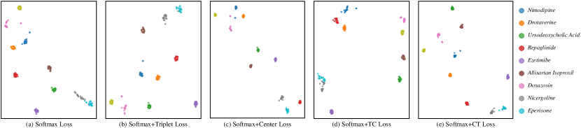
Figure 5: The t-SNE visualization of feature representations generated by models trained with different losses. It can be found that compared with feature representations learned by (a) Softmax loss, (b) Triplet loss obtains better inter-class separability; (c) Center loss achieves better intra-class compactness. (d) Triplet-Center loss inherits the advantages of both (b) and (c); (e) Center-Triplet loss further promotes inter-class separability and intra-class compactness.

To better observe the discriminative ability of the deep features learned by these loss functions, we employ the t-SNE to visualize the features learned by the aforementioned loss functions on the FCPill dataset. As is shown in Fig 5, some characteristics among these losses can be found. First, compared with the Softmax loss function, the feature representations of the same class are better separated after the import of the Triplet loss function. This phenomenon can be easily observed between the samples of Nicergoline and Eperisone in Fig. 5(a) and Fig. 5(b). Second, the introduction of the Center loss function promotes intra-class compactness. This improvement can be found among Fig. 5(a) and Fig. 5(c), such as the samples of Repaglinide, Allisartan Isoproxil, and Nicergoline. Third, although the joint supervision of Softmax loss and TC loss inherits some advantages from Triplet loss and Center loss, it still can be discovered that the intra-class and inter-class variances perform worse than that of Center loss on the proposed FCPill dataset. This phenomenon can be discovered between the samples of Nicergoline and Eperisone in Fig. 5(c) and Fig. 5(d). Nevertheless, our proposed CT loss demonstrates outstanding performance. It fully inherits the small intra-class and larger inter-class variance from the Center loss and the Triplet loss. This characteristics can be easily found among the samples of Drotaverine, Repaglinide, Nicergoline, and Eperisone in Fig. 5(b), Fig. 5(c), and Fig. 5(e). These visualizations of learned features sufficiently prove the effectiveness of our proposed CT loss function.

V-C Comparison with Other Methods

To prove the effectiveness of our proposed few-shot class-incremental pill recognition framework, we compare it with other representative and state-of-the-art methods on the FCPill dataset and the miniCURE dataset. The related methods includes CEC [32], iCaRL [29], EEIL [43], NCM [44], BiC [45], LwM [46], DR [47] and PODNet [48], and their codes are provided by https://github.com/icoz69/CEC-CVPR2021 and https://github.com/zhchuu/continual-learning-reproduce. The comparison results on the FCPill dataset are provided in Fig. 6(a) and Tab. III. It can be found that our proposed framework outperforms other methods. Specifically, our proposed framework obtains the highest accuracy on all sessions. Compared with the state-of-the-art method, CEC, our method obtains an accuracy of $91.89\%$ on the base session, which is $2.71\%$ higher than that of CEC. Regarding the accuracy improvement of the final session, our method is $1.11\%$ higher than CEC. Besides, our method achieves an average accuracy of $87.29\%$ across all sessions, which outperforms CEC by $1.7\%$. Additionally, the comparison results on the miniCURE also demonstrate the effectiveness of our framework. As the details are shown in Fig. 6(b) and Tab. IV, our proposed framework achieves the best performance on all sessions except session $1$. Our method’s accuracy obtained on the base session is $84.37$, which is $0.42\%$ higher than that of CEC. The accuracy obtained on the final session by our method is $71.54\%$, which is $2.40\%$ higher than that of CEC. Besides, in terms of the average accuracy across all sessions, our method obtains an accuracy of $71.54\%$, which outperforms CEC by $1.66\%$. Therefore, our method demonstrates the effectiveness on the few-shot class-incremental pill recognition task.

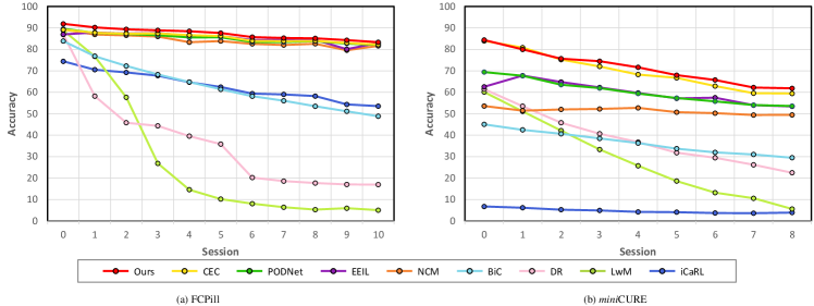
Figure 6: The comparison results between our proposed framework and other representative methods on the FCPill dataset and the miniCURE dataset. (a) shows the results on the FCPill dataset; (b) shows the results on the miniCURE. (In %)

TABLE III: The comparison results between our proposed framework and other representative methods on the FCPill dataset. Average Acc. denotes the average accuracy on all sessions. F. Acc. Impro. denotes the improvement of the accuracy on the final session. (In %)

Method	Sessions											Average Acc.	F. Acc. Impro.
	0	1	2	3	4	5	6	7	8	9	10
iCaRL [29]	74.41	70.52	69.24	67.76	64.67	62.45	59.36	59.00	58.21	54.34	53.52	63.04	+29.82
LwM [46]	88.85	76.72	57.62	26.84	14.59	10.21	8.06	6.40	5.29	5.96	5.06	27.78	+78.28
DR [47]	86.91	58.21	45.79	44.34	39.57	35.82	20.22	18.60	17.68	17.03	16.95	36.47	+66.39
BiC [45]	83.85	76.82	72.26	68.28	64.78	61.39	58.16	56.05	53.48	51.13	48.83	63.18	+34.51
NCM [44]	89.24	86.92	86.52	85.98	83.34	83.87	82.55	82.03	82.61	79.57	81.62	84.02	+1.72
EEIL [43]	86.98	87.86	87.35	87.64	86.28	86.19	84.36	84.46	84.46	80.06	83.03	85.33	+0.31
PODNet [48]	89.58	87.69	87.16	86.58	85.57	85.62	83.46	83.41	83.82	82.69	82.11	85.24	+1.23
CEC [32]	89.18	87.74	87.33	87.41	86.64	86.25	83.96	83.83	83.96	83.02	82.24	85.59	+1.11
Ours	91.89	90.22	89.35	88.86	88.45	87.62	85.73	85.29	85.14	84.28	83.34	87.29

TABLE IV: The comparison results between our proposed framework and other representative methods on the miniCURE dataset. (In %)

Method	Sessions									Average Acc.	F. Acc. Impro.
	0	1	2	3	4	5	6	7	8
iCaRL [29]	6.76	6.19	5.27	4.92	4.24	4.11	3.71	3.63	3.92	4.75	+57.91
LwM [46]	60.11	51.09	42.12	33.35	25.73	18.62	13.21	10.59	5.61	28.94	+56.22
DR [47]	61.43	53.51	45.81	40.66	36.76	31.84	29.47	26.18	22.49	38.68	+39.34
BiC [45]	45.05	42.48	40.63	38.47	36.3	33.72	31.99	30.99	29.5	36.57	+32.33
NCM [44]	53.57	51.44	51.98	52.23	52.71	50.71	50.26	49.41	49.44	51.31	+12.39
EEIL [43]	62.53	67.77	64.77	62.23	59.69	57.16	57.48	53.98	53.39	59.89	+8.44
PODNet [48]	69.4	67.67	63.51	61.94	59.39	57.3	55.76	54.04	53.57	60.29	+8.26
CEC [32]	83.95	80.81	75.22	72.04	68.26	66.72	62.90	59.58	59.43	69.88	+2.40
Ours	84.37	79.95	75.65	74.48	71.63	67.97	65.74	62.21	61.83	71.54

V-D Evaluation of Different Backbones

To evaluate the influence of different backbones, we conduct a comparison experiment based on different backbones on the FCPill dataset. The backbones we used for evaluation include ResNet-18, ResNet-32, ResNet-50, VGG-16, MobileNet-V3 (large), DenseNet-161, EfficientNet-B2, and Vision Transformer (ViT-B/16). To make a fair comparison, the backbones we used are also pre-trained by ImageNet. All the backbones are downloaded directly from Torchvision 0.12.0. As the comparison results are provided in Tab. V, we can find that EfficientNet-B2 achieves the best performance. It obtains the best classification performance on all sessions except the base session with an average accuracy of $89.30\%$. Compared with ResNet-18, EfficientNet-B2 achieves an accuracy of $92.91\%$ on the base session, which is $1.02\%$ higher than that of ResNet-18. Regarding the accuracy improvement of the final session, EfficientNet-B2 is $2.38\%$ higher than ResNet-18. Besides, regarding the average accuracy across all sessions, it also obtains an improvement of $2.01\%$ than ResNet-18. Moreover, from the results shown in Tab. III and Tab. V, it can be found that the proposed framework based on EfficientNet-B2 significantly outperforms the state-of-the-art methods on the FCPill dataset. For instance, the average accuracy of the proposed framework based on EfficientNet-B2 is $3.71\%$ higher than that of CEC, and the accuracy improvement of the final session reached by the proposed framework based on EfficientNet-B2 is $3.48\%$ higher than that of CEC. Therefore, using EfficientNet-B2 as the backbone of our framework can further improve the performance.

TABLE V: The comparison results between different backbones on the FCPill dataset. (In %)

Method	Sessions											Average Acc.	F. Acc. Impro.
	0	1	2	3	4	5	6	7	8	9	10
VGG-16	90.66	89.13	87.82	87.08	86.30	85.47	83.69	83.17	82.78	82.19	81.26	85.41	+4.46
ResNet-32	91.11	89.54	88.86	88.91	88.29	87.22	85.37	84.81	84.73	83.92	83.08	86.89	+2.23
ResNet-50	90.97	89.56	88.61	88.48	88.38	87.21	85.22	84.90	84.66	83.93	83.20	86.83	+2.11
ResNet-18	91.89	90.22	89.35	88.86	88.45	87.62	85.73	85.29	85.14	84.28	83.34	87.29	+1.96
ViT-B/16	92.41	91.54	90.86	90.65	90.63	89.65	87.18	86.88	86.79	85.97	85.16	88.88	+0.56
MobileNet-V3	93.19	91.67	91.05	90.66	90.25	89.68	87.46	87.19	87.13	86.27	85.30	89.08	+0.42
DenseNet-161	92.05	90.85	90.41	90.26	89.85	88.87	87.12	86.76	86.89	86.38	85.31	88.61	+0.41
EfficientNet-B2	92.91	91.96	91.29	90.77	90.74	89.90	87.81	87.51	87.17	86.53	85.72	89.30

VI Conclusion

In this paper, we propose a novel few-shot class-incremental pill recognition framework to deal with the challenges of continuously increasing categories of pills and insufficient data annotation in practical application scenarios. We adopt the decoupled learning strategy of representations and classifiers in this framework. In learning representations, we propose the novel CT loss function based on the Center loss function and the Triplet loss function to train the backbone. This loss function directly considers the relationships between different class centers, which can promote intra-class compactness and inter-class separability. Besides, we propose a specialized pseudo pill image construction strategy to train the GAT adaptation module for classifier learning. To evaluate the effectiveness of our framework, we construct two pill image datasets for FSCIL. The first dataset, FCPill, is sampled from eight groups of pill image data collected from seven hospitals in five Chinese cities, and it contains 144 base and 100 new classes. The second dataset, called miniCURE, is sampled from the public CURE dataset and includes 91 base and 80 new classes. Our experimental results show that our framework outperforms other state-of-the-art methods.

References

- [1] T. T. Mac, “Application of improved yolov3 for pill manufacturing system,” IFAC-PapersOnLine, vol. 54, no. 15, pp. 544–549, 2021.
- [2] Y.-B. Lee, U. Park, A. K. Jain, and S.-W. Lee, “Pill-id: Matching and retrieval of drug pill images,” Pattern Recognition Letters, vol. 33, no. 7, pp. 904–910, 2012.
- [3] Y.-B. Lee, U. Park, and A. K. Jain, “Pill-id: Matching and retrieval of drug pill imprint images,” in ICPR. IEEE, 2010, pp. 2632–2635.
- [4] J. Yu, Z. Chen, S.-i. Kamata, and J. Yang, “Accurate system for automatic pill recognition using imprint information,” IET Image Processing, vol. 9, no. 12, pp. 1039–1047, 2015.
- [5] S. Suntronsuk and S. Ratanotayanon, “Automatic text imprint analysis from pill images,” in 2017 9th International Conference on Knowledge and Smart Technology (KST). IEEE, 2017, pp. 288–293.
- [6] Y. F. Wong, H. T. Ng, K. Y. Leung, K. Y. Chan, S. Y. Chan, and C. C. Loy, “Development of fine-grained pill identification algorithm using deep convolutional network,” Journal of Biomedical Informatics, vol. 74, pp. 130–136, 2017.
- [7] Y.-Y. Ou, A.-C. Tsai, J.-F. Wang, and J. Lin, “Automatic drug pills detection based on convolution neural network,” in 2018 International Conference on Orange Technologies (ICOT). IEEE, 2018, pp. 1–4.
- [8] Y.-Y. Ou, A.-C. Tsai, X.-P. Zhou, and J.-F. Wang, “Automatic drug pills detection based on enhanced feature pyramid network and convolution neural networks,” IET Computer Vision, vol. 14, no. 1, pp. 9–17, 2020.
- [9] W.-J. Chang, L.-B. Chen, C.-H. Hsu, C.-P. Lin, and T.-C. Yang, “A deep learning-based intelligent medicine recognition system for chronic patients,” IEEE Access, vol. 7, pp. 44 441–44 458, 2019.
- [10] N. Larios Delgado, N. Usuyama, A. K. Hall, R. J. Hazen, M. Ma, S. Sahu, and J. Lundin, “Fast and accurate medication identification,” NPJ Digital Medicine, vol. 2, no. 1, pp. 1–9, 2019.
- [11] S. Ling, A. Pastor, J. Li, Z. Che, J. Wang, J. Kim, and P. L. Callet, “Few-shot pill recognition,” in CVPR, 2020, pp. 9789–9798.
- [12] L. Tan, T. Huangfu, L. Wu, and W. Chen, “Comparison of retinanet, ssd, and yolo v3 for real-time pill identification,” BMC Medical Informatics and Decision Making, vol. 21, no. 1, pp. 1–11, 2021.
- [13] N. Pornbunruang, V. Tanjantuk, and T. Titijaroonroj, “Drugtionary: Drug pill image detection and recognition based on deep learning,” in International Conference on Computing and Information Technology. Springer, 2022, pp. 43–52.
- [14] H.-J. Kwon, H.-G. Kim, S.-W. Jung, S.-H. Lee et al., “Deep learning and detection technique with least image-capturing for multiple pill dispensing inspection,” Journal of Sensors, vol. 2022, 2022.
- [15] Y. Wang, Q. Yao, J. T. Kwok, and L. M. Ni, “Generalizing from a few examples: A survey on few-shot learning,” ACM Computing Surveys, vol. 53, no. 3, pp. 1–34, 2020.
- [16] H. Gao, J. Xiao, Y. Yin, T. Liu, and J. Shi, “A mutually supervised graph attention network for few-shot segmentation: The perspective of fully utilizing limited samples,” IEEE Transactions on Neural Networks and Learning Systems, pp. 1–13, 2022.
- [17] W.-H. Li, X. Liu, and H. Bilen, “Cross-domain few-shot learning with task-specific adapters,” in CVPR, 2022, pp. 7161–7170.
- [18] D. A. Ganea, B. Boom, and R. Poppe, “Incremental few-shot instance segmentation,” in CVPR, 2021, pp. 1185–1194.
- [19] C. Xu, Y. Fu, C. Liu, C. Wang, J. Li, F. Huang, L. Zhang, and X. Xue, “Learning dynamic alignment via meta-filter for few-shot learning,” in CVPR, 2021, pp. 5182–5191.
- [20] H. Zhu and P. Koniusz, “Ease: Unsupervised discriminant subspace learning for transductive few-shot learning,” in CVPR, 2022, pp. 9078–9088.
- [21] G. Koch, R. Zemel, R. Salakhutdinov et al., “Siamese neural networks for one-shot image recognition,” in ICML Deep Learning Workshop, vol. 2, 2015, p. 0.
- [22] D.-W. Zhou, F.-Y. Wang, H.-J. Ye, L. Ma, S. Pu, and D.-C. Zhan, “Forward compatible few-shot class-incremental learning,” in CVPR, 2022, pp. 9046–9056.
- [23] H. Zhao, H. Wang, Y. Fu, F. Wu, and X. Li, “Memory-efficient class-incremental learning for image classification,” IEEE Transactions on Neural Networks and Learning Systems, vol. 33, no. 10, pp. 5966–5977, 2022.
- [24] R. Aljundi, F. Babiloni, M. Elhoseiny, M. Rohrbach, and T. Tuytelaars, “Memory aware synapses: Learning what (not) to forget,” in ECCV, 2018, pp. 139–154.
- [25] F. Zenke, B. Poole, and S. Ganguli, “Continual learning through synaptic intelligence,” in ICML, 2017, pp. 3987–3995.
- [26] Z. Li and D. Hoiem, “Learning without forgetting,” IEEE Transactions on Pattern Analysis and Machine Intelligence, vol. 40, no. 12, pp. 2935–2947, 2017.
- [27] E. Belouadah and A. Popescu, “Il2m: Class incremental learning with dual memory,” in ICCV, 2019, pp. 583–592.
- [28] F. Zhu, X.-Y. Zhang, C. Wang, F. Yin, and C.-L. Liu, “Prototype augmentation and self-supervision for incremental learning,” in CVPR, 2021, pp. 5871–5880.
- [29] S.-A. Rebuffi, A. Kolesnikov, G. Sperl, and C. H. Lampert, “icarl: Incremental classifier and representation learning,” in CVPR, 2017, pp. 2001–2010.
- [30] X. Tao, X. Hong, X. Chang, S. Dong, X. Wei, and Y. Gong, “Few-shot class-incremental learning,” in CVPR, 2020, pp. 12 183–12 192.
- [31] Z. Wang, L. Liu, Y. Duan, and D. Tao, “Sin: Semantic inference network for few-shot streaming label learning,” IEEE Transactions on Neural Networks and Learning Systems, pp. 1–14, 2022.
- [32] C. Zhang, N. Song, G. Lin, Y. Zheng, P. Pan, and Y. Xu, “Few-shot incremental learning with continually evolved classifiers,” in CVPR, 2021, pp. 12 455–12 464.
- [33] X. He, Y. Zhou, Z. Zhou, S. Bai, and X. Bai, “Triplet-center loss for multi-view 3d object retrieval,” in CVPR, 2018, pp. 1945–1954.
- [34] Y. Wen, K. Zhang, Z. Li, and Y. Qiao, “A discriminative feature learning approach for deep face recognition,” in ECCV, 2016, pp. 499–515.
- [35] M. Wang and W. Deng, “Deep face recognition: A survey,” Neurocomputing, vol. 429, pp. 215–244, 2021.
- [36] J. Zhang, C. Li, S. Kosov, M. Grzegorzek, K. Shirahama, T. Jiang, C. Sun, Z. Li, and H. Li, “Lcu-net: A novel low-cost u-net for environmental microorganism image segmentation,” Pattern Recognition, vol. 115, p. 107885, 2021.
- [37] N. Dietler, M. Minder, V. Gligorovski, A. M. Economou, D. A. H. L. Joly, A. Sadeghi, C. H. M. Chan, M. Koziński, M. Weigert, A.-F. Bitbol et al., “A convolutional neural network segments yeast microscopy images with high accuracy,” Nature Communications, vol. 11, no. 1, pp. 1–8, 2020.
- [38] X. Zhou, W. Liang, S. Shimizu, J. Ma, and Q. Jin, “Siamese neural network based few-shot learning for anomaly detection in industrial cyber-physical systems,” IEEE Transactions on Industrial Informatics, vol. 17, no. 8, pp. 5790–5798, 2020.
- [39] D. Shi, M. Orouskhani, and Y. Orouskhani, “A conditional triplet loss for few-shot learning and its application to image co-segmentation,” Neural Networks, vol. 137, pp. 54–62, 2021.
- [40] C.-Y. Wu, R. Manmatha, A. J. Smola, and P. Krahenbuhl, “Sampling matters in deep embedding learning,” in ICCV, 2017, pp. 2840–2848.
- [41] F. Schroff, D. Kalenichenko, and J. Philbin, “Facenet: A unified embedding for face recognition and clustering,” in CVPR, 2015, pp. 815–823.
- [42] H. Oh Song, Y. Xiang, S. Jegelka, and S. Savarese, “Deep metric learning via lifted structured feature embedding,” in CVPR, 2016, pp. 4004–4012.
- [43] F. M. Castro, M. J. Marín-Jiménez, N. Guil, C. Schmid, and K. Alahari, “End-to-end incremental learning,” in ECCV, 2018, pp. 233–248.
- [44] S. Hou, X. Pan, C. C. Loy, Z. Wang, and D. Lin, “Learning a unified classifier incrementally via rebalancing,” in CVPR, 2019, pp. 831–839.
- [45] Y. Wu, Y. Chen, L. Wang, Y. Ye, Z. Liu, Y. Guo, and Y. Fu, “Large scale incremental learning,” in CVPR, 2019, pp. 374–382.
- [46] P. Dhar, R. V. Singh, K.-C. Peng, Z. Wu, and R. Chellappa, “Learning without memorizing,” in CVPR, 2019, pp. 5138–5146.
- [47] S. Hou, X. Pan, C. C. Loy, Z. Wang, and D. Lin, “Lifelong learning via progressive distillation and retrospection,” in ECCV, 2018, pp. 437–452.
- [48] A. Douillard, M. Cord, C. Ollion, T. Robert, and E. Valle, “Podnet: Pooled outputs distillation for small-tasks incremental learning,” in ECCV, 2020, pp. 86–102.