Spikingformer: Spike-driven Residual Learning for Transformer-based Spiking Neural Network

Abstract

Spiking neural networks (SNNs) offer a promising energy-efficient alternative to artificial neural networks, due to their event-driven spiking computation. However, state-of-the-art deep SNNs (including Spikformer and SEW ResNet) suffer from non-spike computations (integer-float multiplications) caused by the structure of their residual connection. These non-spike computations increase SNNs’ power consumption and make them unsuitable for deployment on mainstream neuromorphic hardware, which only supports spike operations. In this paper, we propose a hardware-friendly spike-driven residual learning architecture for SNNs to avoid non-spike computations. Based on this residual design, we develop Spikingformer, a pure transformer-based spiking neural network. We evaluate Spikingformer on ImageNet, CIFAR10, CIFAR100, CIFAR10-DVS and DVS128 Gesture datasets, and demonstrate that Spikingformer outperforms the state-of-the-art in directly trained pure SNNs as a novel advanced backbone (75.85$\%$ top-1 accuracy on ImageNet, + 1.04$\%$ compared with Spikformer). Furthermore, our experiments verify that Spikingformer effectively avoids non-spike computations and significantly reduces energy consumption by 57.34$\%$ compared with Spikformer on ImageNet. To our best knowledge, this is the first time that a pure event-driven transformer-based SNN has been developed. Codes will be available at Spikingformer.

1 Introduction

Being regarded as the third generation of neural network [1], the brain-inspired Spiking Neural Networks (SNNs) are potential competitors to Artificial Neural Networks (ANNs) due to their high biological plausibility, event-driven property and low power consumption on neuromorphic hardware [2]. In particular, the utilization of binary spike signals allows SNNs to adopt low-power accumulation (AC) instead of the traditional high-power multiply-accumulation (MAC), leading to significant energy efficiency gains and making SNNs increasingly popular [3].

As SNNs get deeper, their performance has been significantly improved [4, 5, 6, 7, 8, 9, 10]. ResNet with skipping connection has been extensively studied to extend the depth of SNNs [5, 8]. Recently, SEW ResNet [5], a representative convolution-based SNN, easily implements identity mapping and overcomes the vanishing/exploding gradient problems of Spiking ResNet [11]. SEW ResNet is the first deep SNN directly trained with more than 100 layers. Spikformer [8], a directly trained representative transformer-based SNN with residual connection, is proposed by leveraging both self-attention capability and biological properties of SNNs. It is the first successful exploration for applying flourishing transformer architecture into SNN design, and shows powerful performance. However, both Spikformer and SEW ResNet face the challenge of non-spike computations (integer-float multiplications) caused by ADD residual connection. This not only limits their ability to fully leverage the benefits of event-driven processing in energy efficiency, but also makes it difficult to deploy and optimize their performance on neuromorphic hardware [12, 3].

Developing a pure SNN to address the challenge of non-spike computation in Spikformer and SEW ResNet while maintaining high-performance is extremely critical. In this paper, inspired by the architecture design of Binary Neural Network (BNN) [13, 14, 15, 16], we propose Spike-driven Residual Learning architecture for SNN to avoid the non-spike computations. Based on this residual design, we develop a pure transformer-based spiking neural network, named Spikingformer. We evaluate the performance of Spikingformer on static dataset ImageNet[17], CIFAR[18] (including CIFAR10 and CIFAR100) and neuromorphic datasets (including CIFAR10-DVS and DVS128 Gesture). The experimental results show that Spikingformer effectively avoids integer-float multiplications in Spikformer. In addition, as a novel advanced SNN backbone, Spikingformer outperforms Spikformer in all above datasets by a large margin (e.g. + 1.04$\%$ on ImageNet, + 1.00$\%$ on CIFAR100).

2 Related Work

2.1 Convolution-based Spiking Neural Network

There are two mainstream methods to obtain deep convolution-based SNN models: ANN-to-SNN conversion and direct training through surrogate gradient.

ANN-to-SNN Conversion. In ANN-to-SNN conversion [19, 20, 21, 22, 23, 24], a pre-trained ANN is converted to a SNN by replacing the ReLU activation layers with spiking neurons and adding scaling operations like weight normalization and threshold balancing. This conversion process suffers from long converting time steps and constraints on the original ANN design.

Direct Training through Surrogate Gradient. In the field of direct training, SNNs are unfolded over simulation time steps and trained with backpropagation through time [25, 26]. Due to the non-differentiability of spiking neurons, surrogate gradient method is employed for backpropagation [27, 28]. SEW ResNet[5] is a representative convolution-based SNN model by direct training, and is the first to increase the number of layers in SNNs to be larger than 100. However, the ADD gate in residual connections of SEW ResNet produces non-spike computations of integer-float multiplications in deep convolution layers. [3] has identified the problem of non-spike computations in SEW ResNet and Spikformer, and attempts to solve it through adding an auxiliary accumulation pathway during training and removing it during inference. This strategy needs tedious extra operations and results in a significant performance degradation compared with the original models.

2.2 Transformer-based Spiking Neural Network.

Most existing SNNs borrow architectures from convolutional neural networks (CNNs), so their performance is limited by the performance of CNNs. The transformer architecture, originally designed for natural language processing [29], has achieved great success in many computer vision tasks, including image classification [30, 31], object detection [32, 33, 34] and semantic segmentation [35, 36]. The structure of transformer leads to promise for a novel kind of SNNs, with great potential to break through the bottleneck of SNNs’ performance. So far, two main related works: Spikformer[8] and Spikeformer[37] have proposed spiking neural networks based on transformer architecture. Although Spikeformer replaces the activation function used in the feedforward layers with a spiking activation function, there are still a lot of non-spike operations remained, including floating point multiplication, division, exponential operation. Spikformer proposes a novel Spiking Self Attention (SSA) module by using spike-form Query, Key, and Value without softmax, and achieves state-of-the-art performances on many datasets. However, the structure of Spikformer with residual connection still contains non-spike computation. In our study, we adopt the SSA module from Spikformer, and modify the residual structure to be purely event-driven, which is hardware-friendly and energy efficient while improving performance.

3 Methods

3.1 Drawbacks of Spikformer and SEW ResNet

At present, Spikformer [8] is the representative work combining deep SNNs with transformer architecture, while SEW ResNet [5] is the representative work of convolution-based deep SNNs. The residual learning plays an extremely important role in both Spikformer and SEW ResNet, but the ADD residual connections in Spikformer and SEW ResNet lead to non-spike computation (integer-float multiplications), which are not event-driven computation. As shown in Fig.1(a), the residual learning of Spikformer and SEW ResNet could be formulated as follows:

$$O_{l}=\operatorname{SN}_{l}(\operatorname{ConvBN}_{l}(O_{l-1}))+O_{l-1}=S_{l}+O_{l-1},$$ (1)

$$O_{l+1}=\operatorname{SN}_{l+1}(\operatorname{ConvBN}_{l+1}(O_{l}))+O_{l}=S_{l+1}+O_{l}.$$ (2)

where $S_{l}$ denotes the residual mapping learned as $S_{l}=\operatorname{SN}(\operatorname{ConvBN}(O_{l-1}))$. This residual design inevitably brings in non-spike data and thus MAC operations in the next layer / block. In particular, $S_{l}$ and $O_{l-1}$ are spike signals, and their output $O_{l}$ are non-spike signal whose range is $\{0,1,2\}$. Non-spike data destructs event-driven computation in the next convolution layer when computing $S_{l+1}$ of $O_{l+1}$. As the depth of the network increases, the range of non-spike data values transmitted to the deeper layer of the network will also expand. In our implementations of Spikformer, the range of the non-spike data could increase to $\{0,1,2,...,16\}$ when testing Spikormer-8-512 on ImageNet 2012. Obviously, the range of non-spike data is approximately proportional to the number of residual blocks in Spikformer and SEW ResNet.

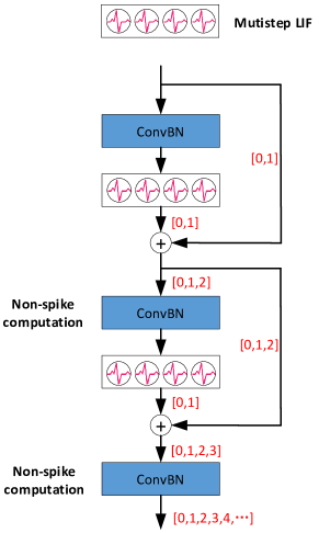
(a) Spikformer, SEW ResNet

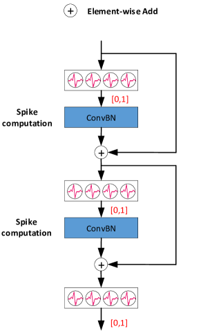
(b) Spikingformer (Ours)

Figure 1: The residual learning in Spikformer, SEW ResNet and Spikingformer (Ours). 1(a) shows the residual learning of Spikformer and SEW ResNet, which contain non-spike computation (integer-float multiplications) in $\operatorname{ConvBN}$ layer. 1(b) shows our proposed spike-driven residual learning in Spikingformer, which could effectively avoid floating-point multiplication and integer-float multiplications, following the spike-driven principle. Note that Mutistep LIF is spike neuron Leaky Integrate-and-Fire (LIF) model [5, 8] with time steps $T>1$. Same with Spikformer, $T$ is an independent dimension for spike neuron layer. In other layers, it is merged with the batch size. We use $\operatorname{ConvBN}$ to represent a convolution layer and its subsequent BN layer in this work.

In fact, integer-float multiplications are usually implemented in the same way as floating-point multiplication in hardware. In this case, the network will incur high energy consumption, approaching to the energy consumption of ANNs with the same structure, which is unacceptable for SNNs.

3.2 Spike-driven Residual Learning in Spikingformer

Fig.1(b) shows our proposed spike-driven residual learning in Spikingformer. It could effectively avoid floating-point multiplications and integer-float multiplications, following the spike-driven principle. The spike-driven residual learning could be easily formulated as follows:

$$O_{l}=\operatorname{ConvBN}_{l}(\operatorname{SN}_{l}(O_{l-1}))+O_{l-1}=S_{l}+O_{l-1},$$ (3)

$$O_{l+1}=\operatorname{ConvBN}_{l+1}(\operatorname{SN}_{l+1}(O_{l}))+O_{l}=S_{l+1}+O_{l}.$$ (4)

We proposed $\operatorname{SN}\text{-}\operatorname{ConvBN}$ for residual learning in replacement of $\operatorname{ConvBN}\text{-}\operatorname{SN}$ in Spikformer and SEW ResNet. In our structure, $S_{l}+O_{l-1}$ belongs to floating point addition operation, which is same as the addition operation in $\operatorname{SN}$ layer. Floating point addition operation is the most essential operation of SNN. Obviously, the output $O_{l}$ is also floating point and will pass through a $\operatorname{SN}$ layer before participating in the next $\operatorname{ConvBN}$ computation. Therefore, the pure spike-form feature will be generated after the processing of $\operatorname{SN}$ layer and the computation of $\operatorname{ConvBN}$ layer will become pure floating point addition operation, following spike-driven principle and reducing energy consumption vastly.

3.3 Spikingformer Architecture

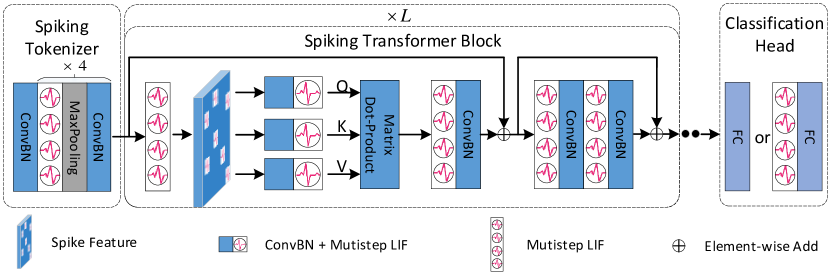
Figure 2: The overview of Spikingformer, which consists of a Spiking Tokenizer, several Spiking Transformer Blocks and a Classification Head.

We propose Spikingformer, which is a novel and pure transformer-based spiking neural network through integrating spike-driven residual blocks. In this section, the details of Spikingformer are discussed. The pipeline of Spikingformer is shown in Fig.2.

Our proposed Spikingformer contains a Spiking Tokenizer (ST), several Spiking Transformer Blocks and a Classification Head. Given a 2D image sequence $I\in\mathbb{R}^{T\times C\times H\times W}$ (Note that $C\text{=}3$ in static datasets like ImageNet 2012, $C\text{=}2$ in neuromorphic datasets like DVS-Gesture), we use the Spiking Tokenizer block for downsampling and patch embedding, where the inputs can be projected as spike-form patches $X\in\mathbb{R}^{T\times N\times D}$. Obviously, the first layer of Spiking Tokenizer also play a spike encoder role when taking static images as input. After Spiking Tokenizer, the spiking patches $X_{0}$ will pass to the $L$ Spiking Transformer Blocks. Similar to the standard ViT encoder block, a Spiking Transformer Block contains a Spiking Self Attention (SSA) [8] and a Spiking MLP block. In the last, a fully-connected-layer (FC) is used for Classification Head. Note that we use a global average-pooling (GAP) before the fully-connected-layer to reduce the parameters of FC and improve the classification classifation capability of Spikingformer.

$$X=\operatorname{ST}(I),\quad I\in\mathbb{R}^{T\times C\times H\times W},X\in\mathbb{R}^{T\times N\times D}$$ (5)

$$X_{l}^{\prime}=\operatorname{SSA}\left(X_{l-1}\right)+X_{l-1},X_{l}^{\prime}\in\mathbb{R}^{T\times N\times D},l=1\ldots L$$ (6)

$$X_{l}=\operatorname{SMLP}\left(X_{l}^{\prime}\right)+X_{l}^{\prime},X_{l}\in\mathbb{R}^{T\times N\times D},l=1\ldots L$$ (7)

$$Y=\operatorname{FC}\left(\operatorname{GAP}\left(X_{L}\right)\right)\quad or\quad Y^{\prime}=\operatorname{FC}\left(\operatorname{GAP}(\operatorname{SN}\left(X_{L}\right))\right)$$ (8)

Spiking Tokenizer. As shown in Fig.2, Spiking Tokenizer mainly contains two functions: 1) convolutional spiking patch embedding, and 2) downsampling to project the feature map into a smaller fixed size. The spiking patch embedding is similar to the convolutional stream in Vision Transformer [38, 39], where the dimension of spike-form feature channels gradually increased in each convolution layer and finally matches the embedding dimension of patches. In addition, the first layer of Spiking Tokenizer is utilized as a spike encoder when using static images as input. As shown in Eq. 9 and Eq. 10, the convolution part of $\operatorname{ConvBN}$ represents the 2D convolution layer (stride-1, 3 × 3 kernel size). $\operatorname{MP}$ and $\operatorname{SN}$ represent maxpooling (stride-2) and mutistep spiking neuron, respectively. Eq. 9 is used for Spiking Patch Embedding without Downsampling (SPE), Eq. 10 is Spiking Patch Embedding with Downsampling (SPED). We could use multiple SPEs or SPEDs for specific classification tasks with different downsampling requirements. For example, we use 4 SPEDs for ImageNet 2012 dataset classification with input size as 224*224 (using 16 times downsampling). we use 2 SPEs and 2 SPEDs for CIFAR datset classification with input size as 32*32 (using 4 times downsampling). After the processing of the Spiking Tokenizer block, the input $I$ is split into an image patch sequence $X\in\mathbb{R}^{T\times N\times D}$.

$$I_{i}=\operatorname{ConvBN}(\operatorname{SN}(I))$$ (9)

$$I_{i}=\operatorname{ConvBN}(\operatorname{MP}(\operatorname{SN}(I)))$$ (10)

Spiking Transformer Block. A Spiking Transformer Block contains Spiking Self Attention (SSA) mechanism and Spiking MLP block. our Spiking Self Attention part is similar with SSA in Spikformer [8], which is a pure spike-form self attention. However, we make some modifications: 1) we change the spiking neuron layer position according to our proposed spike-driven residual mechanism, avoiding the multiplication of integers and floating-point weights. 2) we choose $\operatorname{ConvBN}$ in replacement of $LinearBN$ (linear layer and batch normalization) in Spikformer. Therefore, the SSA in Spikingformer can be formulated as follows:

$$X^{\prime}=\operatorname{SN}(X),$$ (11)

$$Q=\operatorname{SN}_{Q}(\operatorname{ConvBN}_{Q}(X^{\prime})),K=\operatorname{SN}_{K}(\operatorname{ConvBN}_{K}(X^{\prime})),V=\operatorname{SN}_{V}(\operatorname{ConvBN}_{V}(X^{\prime}))$$ (12)

$$\operatorname{SSA}(Q,K,V)=\operatorname{ConvBN}(\operatorname{SN}(QK^{\mathrm{T}}V*s))$$ (13)

where $Q,K,V\in\mathbb{R}^{T\times N\times D}$ are pure spike data (only containing 0 and 1). $s$ is the scaling factor as in [8], controlling the large value of the matrix multiplication result. The Spiking MLP block consists of two SPEs which is formulated in Eq.9. Spiking Transformer Block is shown in Fig.2, and it is the main component of Spikingformer.

Classification Head. We use a fully-connected-layer as the classifier behind the last Spiking Transformer Block. In detail, the classifier could be realized in four forms: $\operatorname{AvgPooling}\text{-}\operatorname{FC}$, $\operatorname{SN}\text{-}\operatorname{AvgPooling}\text{-}\operatorname{FC}$, $\operatorname{FC}\text{-}\operatorname{AvgPooling}$, $\operatorname{SN}\text{-}\operatorname{FC}\text{-}\operatorname{AvgPooling}$ and formulated as follows:

$$Y=\operatorname{FC}(\operatorname{AvgPooling}(X_{L}))$$ (14)

$$Y=\operatorname{FC}(\operatorname{AvgPooling}(\operatorname{SN}(X_{L})))$$ (15)

$$Y=\operatorname{AvgPooling}(\operatorname{FC}(X_{L}))$$ (16)

$$Y=\operatorname{AvgPooling}(\operatorname{FC}(\operatorname{SN}(X_{L})))$$ (17)

$\operatorname{AvgPooling}$ after $\operatorname{FC}$ (like $\operatorname{SN}\text{-}\operatorname{FC}\text{-}\operatorname{AvgPooling}$, $\operatorname{FC}\text{-}\operatorname{AvgPooling}$) could be considered as computing the average of neuron firing, a post-processing of network, but in this way $\operatorname{FC}$ usually requires numerous parameters. $\operatorname{AvgPooling}$ before $\operatorname{FC}$ (like $\operatorname{AvgPooling}\text{-}\operatorname{FC}$, $\operatorname{SN}\text{-}\operatorname{AvgPooling}\text{-}\operatorname{FC}$) could effectively reduce parameters compared with the previous ways. Only $\operatorname{SN}\text{-}\operatorname{FC}\text{-}\operatorname{AvgPooling}$ could avoid floating-point multiplication operation, but it needs more $\operatorname{FC}$ parameters than $\operatorname{AvgPooling}\text{-}\operatorname{FC}$ or $\operatorname{SN}\text{-}\operatorname{AvgPooling}\text{-}\operatorname{FC}$. In addition, it also reduces the classification ability of the network. In this paper, we mainly adopt the way of $\operatorname{AvgPooling}$ ahead of $\operatorname{FC}$, and choose $\operatorname{AvgPooling}\text{-}\operatorname{FC}$ as the classifier of Spikingformer by default. Some experimental analysis on the classification head will be discussed in Sec.5.1.

3.4 Theoretical Synaptic Operation and Energy Consumption Calculation

The homogeneity of convolution allows the following BN and linear scaling transformation to be equivalently fused into the convolutional layer with an added bias when deployment [40, 41, 11, 3]. Therefore, when calculating the theoretical energy consumption, the consumption of BN layers could be ignored. We calculate the number of the synaptic operations of spike before calculating theoretical energy consumption for Spikingformer.

$$SOP^{l}=fr\times T\times{FLOPs}^{l}$$ (18)

where $l$ is a block/layer in Spikingformer, $fr$ is the firing rate of the block/layer and $T$ is the simulation time step of spike neuron. ${FLOPs}^{l}$ refers to floating point operations of block/layer $l$, which is the number of multiply-and-accumulate (MAC) operations. And ${SOP}^{l}$ is the number of spike-based accumulate (AC) operations. We estimate the theoretical energy consumption of Spikingformer according to [42, 7, 12, 43, 44, 45, 46]. We assume that the MAC and AC operations are implemented on the 45nm hardware [12], where $E_{MAC}=4.6pJ$ and $E_{AC}=0.9pJ$. The theoretical energy consumption of Spikingformer can be calculated as follows:

$$E_{Spikingformer}^{rgb}=E_{AC}\times\left(\sum_{i=2}^{N}SOP_{\operatorname{Conv}}^{i}+\sum_{j=1}^{M}SOP_{\operatorname{SSA}}^{j}\right)+E_{MAC}\times\left(FLOP_{\operatorname{Conv}}^{1}\right)$$ (19)

$$E_{Spikingformer}^{neuro}=E_{AC}\times\left(\sum_{i=1}^{N}SOP_{\operatorname{Conv}}^{i}+\sum_{j=1}^{M}SOP_{\operatorname{SSA}}^{j}\right)$$ (20)

Eq.19 shows energy consumption of Spikingformer for static datasets with RGB images input. $FLOP_{Conv}^{1}$ is the first layer encoding static RGB images into spike-form. Then the SOPs of $N$ SNN Conv layers and $M$ SSA layers are added together and multiplied by $E_{AC}$. Eq.20 shows energy consumption of Spikingformer for neuromorphic datasets.

4 Experiments

In this section, we carry out experiments on static dataset ImageNet [17], static dataset CIFAR [18] (including CIFAR10 and CIFAR100) and neuromorphic datasets (including CIFAR10-DVS and DVS128 Gesture [47]) to evaluate the performance of Spikingformer. The models for conducting experiments are implemented based on Pytorch [48], SpikingJelly [49] and Timm [50].

Table 1: Results on ImageNet-1k classification. Power is calculated as the average theoretical energy consumption of an image inference on ImageNet, whose detail is shown in Eq19. Same as Spikformer, our Spikingformer-$L$-$D$ represents a Spikingformer model with $L$ spiking transformer blocks and $D$ feature embedding dimensions. OPs refers to SOPs in SNN and FLOPs in ANN. Note that the default input resolution of inference is 224×224.

Methods	Architecture	Param (M)	OPs (G)	Time Step	Energy Con-sumption(mJ)	Top-1 Acc
TET[51]	Spiking-ResNet-34	21.79	-	6	-	64.79
	SEW ResNet-34	21.79	-	4	-	68.00
Spiking ResNet[4]	ResNet-34	21.79	65.28	350	59.30	71.61
	ResNet-50	25.56	78.29	350	70.93	72.75
STBP-tdBN[6]	Spiking-ResNet-34	21.79	6.50	6	6.39	63.72
SEW ResNet[5]	SEW ResNet-34	21.79	3.88	4	4.04	67.04
	SEW ResNet-50	25.56	4.83	4	4.89	67.78
	SEW ResNet-101	44.55	9.30	4	8.91	68.76
	SEW ResNet-152	60.19	13.72	4	12.89	69.26
MS-ResNet[7]	ResNet-104	44.55+	-	5	-	74.21
ANN[8]	Transformer-8-512	29.68	8.33	1	38.34	80.80
Spikformer[8]	Spikformer-8-384	16.81	6.82	4	12.43	70.24
	Spikformer-8-512	29.68	11.09	4	18.82	73.38
	Spikformer-8-768	66.34	22.09	4	32.07	74.81
Spikingformer	Spikingformer-8-384	16.81	3.88	4	4.69(-62.27$\%$)	72.45(+2.21)
	Spikingformer-8-512	29.68	6.52	4	7.46(-60.36$\%$)	74.79(+1.41)
	Spikingformer-8-768	66.34	12.54	4	13.68(-57.34$\%$)	75.85(+1.04)

4.1 ImageNet Classification

ImageNet contains around $1.3$ million $1000$-class images for training and $50,000$ images for validation. The input size of our model on ImageNet is set to the default $224\times 224$. The optimizer is AdamW and the batch size is set to $192$ or $288$ during $310$ training epochs with a cosine-decay learning rate whose initial value is $0.0005$. The scaling factor is $0.125$ when training on ImageNet and CIFAR. Four SPEDs in Spiking Tokenizer splits the image into $196$ $16\times 16$ patches.

Same as Spikformer, We try a variety of models with different embedding dimensions and numbers of transformer blocks for ImageNet, which has been shown in Tab. 1. We also show the comparison of synaptic operations (SOPs) [52] and theoretical energy consumption. On one hand, Spkingformer follows spike-driven computation rules, effectively avoiding floating-point multiplication and integer-float multiplications. The histogram of the input data for each transformer block of Spikingformer and Spikformer is shown in Appendix E of Supplementary Material, our Spikingformer effectively avoids producing non-spike data of non-spike computations in Spikformer. On the other hand, Spikingformer-8-512 achieves 74.79$\%$ top-1 classification accuracy on ImageNet using 4 time steps, significantly outperforms Spikformer-8-512 by 1.41$\%$, outperforms MS-ResNet model by 0.58$\%$ and outperforms SEW ResNet-152 model by 5.53$\%$. Spikingformer-8-512 is with 7.463 mJ theoretical energy consumption, which reduces energy consumption by 60.36$\%$, compared with 18.819 mJ of Spikformer-8-512. Spikingformer-8-768 achieves 75.85$\%$ top-1 classification accuracy on ImageNet using 4 time steps, significantly outperforms Spikformer-8-768 by 1.04$\%$, outperforms MS-ResNet model by 1.64$\%$ and outperforms SEW ResNet-152 model by 6.59$\%$. Spikingformer-8-768 is with 13.678 mJ theoretical energy consumption, which reduces energy consumption by 57.34$\%$, compared with 32.074 mJ of Spikformer-8-768. In addition, we recalculate the energy consumption of Spikformer in Appendix G because the non-spike computation of Spikformer can not be directly calculated by Sec.3.4. The main reason why Spikingformer can significantly reduce energy consumption compared with Spikformer is that Spikingformer could effectively avoid integer-float multiplications, and the secondary reason is that our models have lower firing rate on ImageNet, which is shown in Appendix E.

Table 2: Results on CIFAR10/100 classification. Spikingformer improves network performance in all tasks, compared with Spikformer. Note that Spikingformer-4-384-400E means Spikingformer contains four spiking transformer blocks and 384 feature embedding dimensions, trained with 400 epochs. Other models of Spikingformer are trained with 310 epochs by default, being consistent with Spikformer.

Methods	Architecture	Param (M)	Time Step	CIFAR10 Top-1 Acc	CIFAR100 Top-1 Acc
Hybrid training[53]	VGG-11	9.27	125	92.22	67.87
Diet-SNN[54]	ResNet-20	0.27	10/5	92.54	64.07
STBP[55]	CIFARNet	17.54	12	89.83	-
STBP NeuNorm[56]	CIFARNet	17.54	12	90.53	-
TSSL-BP[57]	CIFARNet	17.54	5	91.41	-
STBP-tdBN[6]	ResNet-19	12.63	4	92.92	70.86
TET[51]	ResNet-19	12.63	4	94.44	74.47
MS-ResNet[7]	ResNet-110	-	-	91.72	66.83
	ResNet-482	-	-	91.90	-
ANN[8]	ResNet-19*	12.63	1	94.97	75.35
	Transformer-4-384	9.32	1	96.73	81.02
Spikformer[8]	Spikformer-4-256	4.15	4	93.94	75.96
	Spikformer-2-384	5.76	4	94.80	76.95
	Spikformer-4-384	9.32	4	95.19	77.86
	Spikformer-4-384-400E	9.32	4	95.51	78.21
Spikingformer	Spikingformer-4-256	4.15	4	94.77(+0.83)	77.43(+1.47)
	Spikingformer-2-384	5.76	4	95.22(+0.42)	78.34(+1.39)
	Spikingformer-4-384	9.32	4	95.61(+0.42)	79.09(+1.23)
	Spikingformer-4-384-400E	9.32	4	95.81(+0.30)	79.21(+1.00)

4.2 CIFAR Classification

CIFAR10/CIFAR100 provides 50, 000 train and 10, 000 test images with 32 × 32 resolution. The difference is that CIFAR10 contains 10 categories for classification, but CIFAR100 contains 100 categories, owning better distinguishing ability for classification algorithm. The batch size of Spikingformer is set to 64. We choose two SPEs and two SPEDs in the Spiking Tokenizer block to split the input image into 64 4 × 4 patches.

The experimental results are shown in Tab.2. From the results, We find that the performance of Spikingformer models surpass all the models of Spikformer with same number of parameters. In CIFAR10, our Spikingformer-4-384-400E achieves 95.81$\%$ classification accuracy, significantly outperforms Spikformer-4-384-400E by 0.30$\%$ and outperforms MS-ResNet-482 by 3.91$\%$. In CIFAR100, Spikingformer-4-384-400E achieves 79.21$\%$ classification accuracy, significantly outperforms Spikformer-4-384-400E by 1.00$\%$ and outperforms MS-ResNet-110 by 12.38$\%$. To the best of our knowledge, our Spikingformer achieves the state-of-the-art in directly trained pure spike-driven SNN model on both CIFAR10 and CIFAR100. ANN-Transformer model is 1.12$\%$ and 1.93$\%$ higher than Spikformer-4-384 for CIFAR10 and CIFAR100, respectively. In this experiment, we also find that the performance of Spikingformer has positive correlation with block numbers, dimensions and training epochs within a certain range in CIFAR dataset.

Table 3: Results on neuromorphic datasets, CIFAR10-DVS and DVS128 Gesture. Note that the result of Spikformer is based on our implementation according to its open-source code.

Method	CIFAR10-DVS		DVS128 Gesture
	Time Step	Acc	Time Step	Acc
LIAF-Net [58]TNNLS-2021	10	70.4	60	97.6
TA-SNN [59]ICCV-2021	10	72.0	60	98.6
Rollout [60]Front. Neurosci-2020	48	66.8	240	97.2
DECOLLE [61]Front. Neurosci-2020	-	-	500	95.5
tdBN [6]AAAI-2021	10	67.8	40	96.9
PLIF [62]ICCV-2021	20	74.8	20	97.6
SEW ResNet [5]NeurIPS-2021	16	74.4	16	97.9
Dspike [63]NeurIPS-2021	10	75.4	-	-
SALT [64]Neural Netw-2021	20	67.1	-	-
DSR [23]CVPR-2022	10	77.3	-	-
MS-ResNet [7]	-	75.6	-	-
Spikformer[8] (Our Implement)	10	78.6	10	95.8
	16	80.6	16	97.9
Spikingformer (Ours)	10	79.9(+1.3)	10	96.2(+0.4)
	16	81.3(+0.7)	16	98.3(+0.4)

4.3 DVS Classification

CIFAR10-DVS Classification. CIFAR10-DVS is a neuromorphic dataset converted from the static image dataset by shifting image samples to be captured by the DVS camera, which provides 9, 000 training samples and 1, 000 test samples. We compare our method with SOTA methods on DVS-Gesture. In detail, we adopt four SPEDs in the Spiking Tokenizer block due to 128*128 image size of CIFAR10-DVS, and adopt 2 spiking transformer blocks with 256 patch embedding dimension. The number of time steps of the spiking neuron is 10 or 16. The number of training epochs is 106, which is the same with Spikformer. The learning rate is initialized to 0.1 and decayed with cosine schedule.

The results of CIFAR10-DVS are shown in Tab.3. Spikingformer achieves 81.3$\%$ top-1 accuracy with 16 time steps and 79.9$\%$ accuracy with 10 time steps, significantly outperforms Spikformer by 1.3$\%$ and 0.7$\%$ respectively. To our best knowledge, our Spikingformer achieves the state-of-the-art in directly trained pure spike-driven SNN models on CIFAR10-DVS.

DVS128 Gesture Classification. DVS128 Gesture is a gesture recognition dataset that contains 11 hand gesture categories from 29 individuals under 3 illumination conditions. The image size of DVS128 Gesture is 128*128. The main hyperparameter setting in DVS128 Gesture classification is the same with CIFAR10-DVS classification. The only difference is that the number of training epoch is set as 200 for DVS Gesture classification, which is the same with Spikformer.

We compare our method with SOTA methods on CIFAR10-DVS in Tab.3. Spikingformer achieves 98.3$\%$ top-1 accuracy with 16 time steps and 96.2$\%$ accuracy with 10 time steps, outperforms Spikformer by 0.4$\%$ and 0.4$\%$ respectively.

5 Discussion

5.1 Further Analysis for Last Layer

Table 4: Discussion results on the last layer of Spikingformer. Spikingformer-$L$-$D$^∗ means Spikingformer with the last layer of $\operatorname{SN}\text{-}\operatorname{AvgPooling}\text{-}\operatorname{FC}$. Spikingformer-$L$-$D$ means Spikingformer with the last layer of $\operatorname{AvgPooling}\text{-}\operatorname{FC}$ by default.

Dataset	Models	Time Step	Top-1 Acc
CIFAR10	Spikingformer-4-384-400E	4	95.81
	Spikingformer-4-384-400E∗	4	95.58
	Spikformer-4-384-400E	4	95.51
CIFAR100	Spikingformer-4-384-400E	4	79.21
	Spikingformer-4-384-400E∗	4	78.39
	Spikformer-4-384-400E	4	78.21

We carry out analysis of the last layer of Spikingformer in CIFAR10 and CIFAR100 dataset to study its impacts, and the results are shown in Tab.4. The last layer has significant impacts on model performances although it only occupies a very small component in Spikingformer. Our experiments show that Spikingformer-$L$-$D^{*}$ with spike signals performs worse than Spikingformer-$L$-$D$ on the whole. This can be attributed to the fact that the $\operatorname{AvgPooling}$ layer of $\operatorname{AvgPooling}\text{-}\operatorname{FC}$ processes floating point numbers, which have stronger classification abilities than spike signals in $\operatorname{SN}\text{-}\operatorname{AvgPooling}\text{-}\operatorname{FC}$. However, Spikingformer-$L$-$D^{*}$ still outperforms Spikformer-$L$-$D$, which uses a $\operatorname{SN}\text{-}\operatorname{AvgPooling}\text{-}\operatorname{FC}$ layer as the classifier. On one hand, Spikingformer effectively avoids integer-float multiplications of Spikformer in residual learning. On the other hand, Spikingformer has better spike feature extraction and classification ability than Spikformer. These results further verify the effectiveness of Spikingformer as a backbone.

5.2 More Discussion for $Activation\text{-}Conv\text{-}BatchNorm$ Paradigm

$Activation\text{-}Conv\text{-}BatchNorm$ is a fundamental building block in Binary Neural Networks (BNN) [13, 14, 15, 16]. MS-ResNet[7] has inherited $Activation\text{-}Conv\text{-}BatchNorm$ in directly trained convolution-based SNNs to successfully extend the depth up to 482 layers on CIFAR10, without experiencing degradation problem. MS-ResNet mainly verifies the ability of $Activation\text{-}Conv\text{-}BatchNorm$ to overcome the problem of gradient explosion/vanishing and performance degradation in convolution-based SNN model. In contrast, to the best of our knowledge, Spikingformer is the first transformer-based SNN model that uses the $Activation\text{-}Conv\text{-}BatchNorm$ paradigm to achieve pure spike-driven computation. This work further validates the effectiveness and fundamentality of $Activation\text{-}Conv\text{-}BatchNorm$ as a basic module in SNN design. Specifically, Spikingformer achieves state-of-the-art performance on five datasets, and outperforms MS-ResNet by a significant margin: for ImageNet, CIFAR10, CIFAR100, CIFAR10-DVS, DVS-Guesture, MS-ResNet (our Spikingformer) achieves 74.21$\%$ (75.85$\%$), 91.90$\%$ (95.81$\%$), 66.83$\%$ (79.21$\%$), 75.6$\%$ (81.3$\%$), - (98.3$\%$), respectively.

6 Conclusion

In this paper, we propose spike-driven residual learning for SNN to avoid non-spike computations in Spikformer and SEW ResNet. Based on this residual design, we develop a pure spike-driven transformer-based spiking neural network, named Spikingformer. We evaluates Spikingformer on ImageNet, CIFAR10, CIFAR100, CIFAR10-DVS and DVS128 Gesture datasets. The experiment results verify that Spikingformer effectively avoids integer-float multiplications in Spikformer. In addition, Spikingformer, as a newly advanced SNN backbone, outperforms Spikformer in all above datasets by a large margin (eg. + 1.04$\%$ on ImageNet, + 1.00$\%$ on CIFAR100). To our best knowledge, Spikingformer is the first pure spike-driven transformer-based SNN model, and achieves state-of-the-art performance on the above datasets in directly trained pure SNN models.

7 Acknowledgment

This work is supported by grants from National Natural Science Foundation of China 62236009 and 62206141.

Appendix

Appendix A Spiking Neuron Model

Spike neuron is the fundamental unit of SNNs, we choose Leaky Integrate-and-Fire (LIF) model as the spike neuron in our work. The dynamics of a LIF neuron can be formulated as follows:

$$H[t]=V[t-1]+\frac{1}{\tau}\left(X[t]-\left(V[t-1]-V_{\text{reset }}\right)\right),$$ (21)

$$S[t]=\Theta\left(H[t]-V_{th}\right),$$ (22)

$$V[t]=H[t](1-S[t])+V_{\text{reset }}S[t]$$ (23)

where $\tau$ is the membrane time constant, and $X[t]$ is the input current at time step $t$. When the membrane potential $H[t]$ exceeds the firing threshold $V_{th}$, the spike neuron will trigger a spike $S[t]$. $\Theta(v)$ is the Heaviside step function, which equals to 1 when $v\geq 0$ and 0 otherwise. $V[t]$ represents the membrane potential after the triggered event, which equals to $H[t]$ if no spike is generated and otherwise equals to the reset potential $V_{reset}$.

Appendix B Theoretical Analysis in Fusion of Convolution and Batch Normalization

Obviously, the binary spikes become floating-point values when it has passed through the convolution layer, which leads to subsequent MAC operations in Batch Normalization (BN) layer. However, the homogeneity of convolution allows the following BN and linear scaling transformation to be equivalently fused into the convolutional layer with an added bias when deployment. In particular, each BN layer and its preceding convolution layer are fused into a convolution $\operatorname{ConvBN}$ layer with a bias vector. The kernel and bias $\{W,B\}$ of $\operatorname{ConvBN}$ can be calculated from $\{W,\mu,\sigma,\gamma,\beta\}$. The process of convolution and batch normalization for an input element $x_{i}$ can be formulated as follow:

$$y_{\operatorname{Conv}}=w_{\operatorname{Conv}}\cdot x_{i}+b_{\operatorname{Conv}}$$ (24)

$$y_{i}=\operatorname{BN}_{\gamma,\beta}\left(x_{i}\right)=\gamma\frac{x_{i}-\mu_{\text{ }}}{\sqrt{\sigma_{\text{ }}^{2}+\varepsilon}}+\beta=\frac{\gamma}{\sqrt{\sigma_{\text{ }}^{2}+\varepsilon}}x_{i}+\beta-\frac{\gamma\cdot\mu_{\text{ }}}{\sqrt{\sigma_{\text{ }}^{2}+\varepsilon}}$$ (25)

Thus in deployment, the batch normalization could be formulated as: $y_{\operatorname{BN}}=w_{\operatorname{BN}}\cdot x_{i}+b_{\operatorname{\operatorname{BN}}}$. Therefore, the above steps could be fused:

$$y_{i}=w_{\operatorname{BN}}(w_{\operatorname{Conv}}\cdot x_{i}+b_{\operatorname{Conv}})+b_{\operatorname{BN}}=w_{\operatorname{BN}}\cdot w_{\operatorname{Conv}}\cdot x_{i}+w_{\operatorname{BN}}b_{\operatorname{Conv}}+b_{\operatorname{BN}}$$ (26)

The equivalent convolution layer $\operatorname{ConBN}$: $W=w_{\operatorname{BN}}\cdot w_{\operatorname{Conv}}$; $B=w_{\operatorname{BN}}\cdot b_{\operatorname{Conv}}+b_{\operatorname{BN}}$.

Appendix C Multi-head Spiking Self Attention in Spikingformer

The Multi-head Spiking Self Attention (MSSA) can be easily formulated as follows:

$$X^{\prime}=\operatorname{SN}(X)$$ (27)

$$Q,K,V=\operatorname{SN}_{q}\left({\operatorname{ConvBN}}_{q}\left(X^{\prime}\right)\right),\operatorname{SN}_{k}\left({\operatorname{ConvBN}_{k}}\left(X^{\prime}\right)\right),\operatorname{SN}_{v}\left({\operatorname{ConvBN}}_{v}\left(X^{\prime}\right)\right)$$ (28)

$$Q^{\prime},K^{\prime},V^{\prime}=\left(q_{1},q_{2},\ldots,q_{H}\right),\left(k_{1},k_{2},\ldots,k_{H}\right),\left(v_{1},v_{2},\ldots,v_{H}\right)$$ (29)

$$\operatorname{MSSA}\left(Q^{\prime},K^{\prime},V^{\prime}\right)={\operatorname{ConvBN}}\left(\operatorname{SN}\left(\left(q_{1}k_{1}^{T}v_{1}*s\right),\ldots,\left(q_{H}k_{H}{}^{T}v_{H}{}*s\right)\right)\right)$$ (30)

where $Q,K,V\in\mathbb{R}^{T\times N\times D}$, and reshaped into H-head form $Q^{\prime},K^{\prime},V^{\prime}\in\mathbb{R}^{T\times H\times N\times d}$ with $D=H\times d$. Note that the scaling factor $s$ in SSA or MSSA is a constant, and can be easily fused into the following spike neuron LIF layer.

Appendix D Supplement of experimental details

In our experiments, we use 8 GPUs when training models on ImageNet, while 1 GPU is used to train other datasets (CIFAR10, CIFAR100, DVS128 Gesture, CIFAR10-DVS). In addition, we adjust the value of membrane time constant $\tau$ in spike neuron when training models on DVS datasets. In direct training SNN models with surrogate function,

$${Sigmoid}(x)=\frac{1}{1+\exp(-\alpha x)}$$ (31)

We select the Sigmoid function as the surrogate function with $\alpha=4$ in all experiments.

Appendix E The Spike Data Statistics of Spikformer and Spikingformer

E.1 Statistics of Spikformer on ImageNet

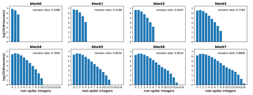
Figure 3: Histogram of the input data of each block in Spikformer-8-512 on ImageNet. The abscissa means non-spike data range with $\{0,1,2,...,16\}$ before $\operatorname{ConvBN}$ layer in the transformer block of Spikformer. The ordinate means the $log$ value (logarithm with a base of 10) of the neuron numbers of each case. Nonzero ratio indicates the ratio of non-zero input units for each block.

Fig.3 shows the histogram of the input data of each block in Spikformer-8-512 on ImageNet. In detail, we obtain the results by running the trained Spikformer-8-512 on whole ImageNet test set. Spikformer-8-512 has 8 transformer block and two resdual connection in every transformer block. Thus, the non-spike numbers can be accumulated up to 16 in Spikformer-8-512. The visualization further verified our analysis: The residual learning of Spikformer results in non-spike computation (integer-float multiplications) in $\operatorname{ConvBN}$ layer.

E.2 Statistics of Spikingformer on ImageNet

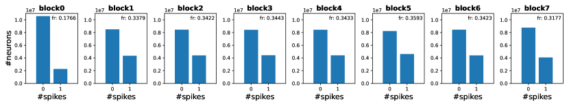
Figure 4: Histogram of the input data of each block in Spikingformer-8-512 on ImageNet. The abscissa means binary spike data with $\{0,1\}$ before $\operatorname{ConvBN}$ layer in the transformer block of Spikingformer. The ordinate means of the neuron numbers of $\{0,1\}$.

As in Sec.E.1, we plot the histogram of the input data of each block in Spikingformer-8-512 on ImageNet in Fig.4. The result show our proposed spike-driven residual learning in Spikingformer could effectively avoid integer-float multiplications common in Spikformer. In addition, $fr$ in Fig.4 represents the fire rate of the input data for each spiking transformer block of Spikingformer. We observe that Spikingformer have lower fire rate on ImageNet compared with Spikformer (Fig.3), which further reduces synaptic operations and thus energy consumption.

Appendix F Additional Results

F.1 Additional Classification Results on CIFAR10

We find that Spikingformer is not completely convergent on some datasets in above tables. For example, after training Spikingformer up to 600 epochs, the accuracy is increased up to 96.04$\%$. In order to compare with other methods in the same conditions, we choose 300 epochs or 400 epochs. Actually, we find SNN models converges much slower than similarly structured ANN models in the practice.

Table 5: Training Spikingformer up to 600 epochs on CIFAR10.

Backbone	Timestep	CIFAR10
Spikingformer-4-384-300E	4	95.61
Spikingformer-4-384-400E	4	95.81
Spikingformer-4-384-600E	4	96.04

Appendix G Energy Consumption Recalculation for Spikformer on ImageNet.

The energy consumption of Spikformer treat the non-spike computation (integer-float multiplications) in $\operatorname{ConvBN}$ layer as binary spike-based accumulate operations. That is obviously unreasonable. Therefore, we provide two ways to recalculate the energy consumption of Spikformer on ImageNet: 1) treating integers $N$ ($N>1$) multiplicating with floats as N times binary spike-based accumulate operations; 2) treating integers $N$ multiplicating with floats as floating point multiplication, which leads to much higher energy consumption. The recalculation in this work is according to the first way.

References

- [1] Wolfgang Maass. Networks of spiking neurons: the third generation of neural network models. Neural networks, 10(9):1659–1671, 1997.
- [2] Kaushik Roy, Akhilesh Jaiswal, and Priyadarshini Panda. Towards spike-based machine intelligence with neuromorphic computing. Nature, 575(7784):607–617, 2019.
- [3] Guangyao Chen, Peixi Peng, Guoqi Li, and Yonghong Tian. Training full spike neural networks via auxiliary accumulation pathway. arXiv preprint arXiv:2301.11929, 2023.
- [4] Yangfan Hu, Huajin Tang, and Gang Pan. Spiking deep residual networks. IEEE Transactions on Neural Networks and Learning Systems, pages 1–6, 2021.
- [5] Wei Fang, Zhaofei Yu, Yanqi Chen, Tiejun Huang, Timoth Masquelier, and Yonghong Tian. Deep Residual Learning in Spiking Neural Networks. In Proceedings of the International Conference on Neural Information Processing Systems (NeurIPS), volume 34, pages 21056–21069, 2022.
- [6] Hanle Zheng, Yujie Wu, Lei Deng, Yifan Hu, and Guoqi Li. Going Deeper With Directly-Trained Larger Spiking Neural Networks. In Proceedings of the AAAI Conference on Artificial Intelligence (AAAI), pages 11062–11070, 2021.
- [7] Yifan Hu, Yujie Wu, Lei Deng, and Guoqi Li. Advancing residual learning towards powerful deep spiking neural networks. arXiv preprint arXiv:2112.08954, 2021.
- [8] Zhaokun Zhou, Yuesheng Zhu, Chao He, Yaowei Wang, Shuicheng YAN, Yonghong Tian, and Li Yuan. Spikformer: When spiking neural network meets transformer. In The Eleventh International Conference on Learning Representations, 2023.
- [9] Ali Lotfi Rezaabad and Sriram Vishwanath. Long short-term memory spiking networks and their applications. In Proceedings of the International Conference on Neuromorphic Systems 2020 (ICONS), pages 1–9, 2020.
- [10] Zulun Zhu, Jiaying Peng, Jintang Li, Liang Chen, Qi Yu, and Siqiang Luo. Spiking graph convolutional networks. In Proceedings of the Thirty-First International Joint Conference on Artificial Intelligence (IJCAI), pages 2434–2440, 2022.
- [11] Yangfan Hu, Huajin Tang, and Gang Pan. Spiking deep residual networks. IEEE Transactions on Neural Networks and Learning Systems, 2021.
- [12] Mark Horowitz. 1.1 computing’s energy problem (and what we can do about it). In 2014 IEEE International Solid-State Circuits Conference Digest of Technical Papers (ISSCC), pages 10–14. IEEE, 2014.
- [13] Zechun Liu, Baoyuan Wu, Wenhan Luo, Xin Yang, Wei Liu, and Kwang-Ting Cheng. Bi-real net: Enhancing the performance of 1-bit cnns with improved representational capability and advanced training algorithm. In Proceedings of the European conference on computer vision (ECCV), pages 722–737, 2018.
- [14] Nianhui Guo, Joseph Bethge, Haojin Yang, Kai Zhong, Xuefei Ning, Christoph Meinel, and Yu Wang. Boolnet: minimizing the energy consumption of binary neural networks. arXiv preprint arXiv:2106.06991, 2021.
- [15] Yichi Zhang, Zhiru Zhang, and Lukasz Lew. Pokebnn: A binary pursuit of lightweight accuracy. In Proceedings of the IEEE/CVF Conference on Computer Vision and Pattern Recognition, pages 12475–12485, 2022.
- [16] Zechun Liu, Zhiqiang Shen, Marios Savvides, and Kwang-Ting Cheng. Reactnet: Towards precise binary neural network with generalized activation functions. In Computer Vision–ECCV 2020: 16th European Conference, Glasgow, UK, August 23–28, 2020, Proceedings, Part XIV 16, pages 143–159. Springer, 2020.
- [17] Jia Deng, Wei Dong, Richard Socher, Li-Jia Li, Kai Li, and Li Fei-Fei. Imagenet: A large-scale hierarchical image database. In Proceedings of the IEEE/CVF Conference on Computer Vision and Pattern Recognition (CVPR), pages 248–255, 2009.
- [18] Alex Krizhevsky. Learning multiple layers of features from tiny images. 2009.
- [19] Yongqiang Cao, Yang Chen, and Deepak Khosla. Spiking deep convolutional neural networks for energy-efficient object recognition. International Journal of Computer Vision, 113(1):54–66, 2015.
- [20] Eric Hunsberger and Chris Eliasmith. Spiking deep networks with lif neurons. arXiv preprint arXiv:1510.08829, 2015.
- [21] Bodo Rueckauer, Iulia-Alexandra Lungu, Yuhuang Hu, Michael Pfeiffer, and Shih-Chii Liu. Conversion of continuous-valued deep networks to efficient event-driven networks for image classification. Frontiers in neuroscience, 11:682, 2017.
- [22] Tong Bu, Wei Fang, Jianhao Ding, PengLin Dai, Zhaofei Yu, and Tiejun Huang. Optimal ann-snn conversion for high-accuracy and ultra-low-latency spiking neural networks. In International Conference on Learning Representations (ICLR), 2021.
- [23] Qingyan Meng, Mingqing Xiao, Shen Yan, Yisen Wang, Zhouchen Lin, and Zhi-Quan Luo. Training High-Performance Low-Latency Spiking Neural Networks by Differentiation on Spike Representation. ArXiv preprint arXiv:2205.00459, 2022.
- [24] Yuchen Wang, Malu Zhang, Yi Chen, and Hong Qu. Signed neuron with memory: Towards simple, accurate and high-efficient ann-snn conversion. In International Joint Conference on Artificial Intelligence, 2022.
- [25] Jun Haeng Lee, Tobi Delbruck, and Michael Pfeiffer. Training deep spiking neural networks using backpropagation. Frontiers in neuroscience, 10:508, 2016.
- [26] Sumit B Shrestha and Garrick Orchard. Slayer: Spike layer error reassignment in time. In Proceedings of the International Conference on Neural Information Processing Systems (NeurIPS), volume 31, 2018.
- [27] Chankyu Lee, Syed Shakib Sarwar, Priyadarshini Panda, Gopalakrishnan Srinivasan, and Kaushik Roy. Enabling spike-based backpropagation for training deep neural network architectures. Frontiers in neuroscience, 14:119, 2020.
- [28] Emre O Neftci, Hesham Mostafa, and Friedemann Zenke. Surrogate gradient learning in spiking neural networks: Bringing the power of gradient-based optimization to spiking neural networks. IEEE Signal Processing Magazine, 36(6):51–63, 2019.
- [29] Ashish Vaswani, Noam Shazeer, Niki Parmar, Jakob Uszkoreit, Llion Jones, Aidan N Gomez, Łukasz Kaiser, and Illia Polosukhin. Attention is all you need. In Proceedings of the International Conference on Neural Information Processing Systems (NeurIPS), volume 30, 2017.
- [30] Alexey Dosovitskiy, Lucas Beyer, Alexander Kolesnikov, Dirk Weissenborn, Xiaohua Zhai, Thomas Unterthiner, Mostafa Dehghani, Matthias Minderer, Georg Heigold, Sylvain Gelly, et al. An image is worth 16x16 words: Transformers for image recognition at scale. In International Conference on Learning Representa- tions (ICLR), 2020.
- [31] Li Yuan, Yunpeng Chen, Tao Wang, Weihao Yu, Yujun Shi, Zi-Hang Jiang, Francis EH Tay, Jiashi Feng, and Shuicheng Yan. Tokens-to-token vit: Training vision transformers from scratch on imagenet. In Proceedings of the IEEE/CVF International Conference on Computer Vision (ICCV), pages 558–567, 2021.
- [32] Nicolas Carion, Francisco Massa, Gabriel Synnaeve, Nicolas Usunier, Alexander Kirillov, and Sergey Zagoruyko. End-to-end object detection with transformers. In Proceedings of the European Conference on Computer Vision (ECCV), pages 213–229. Springer, 2020.
- [33] Xizhou Zhu, Weijie Su, Lewei Lu, Bin Li, Xiaogang Wang, and Jifeng Dai. Deformable detr: Deformable transformers for end-to-end object detection. arXiv preprint arXiv:2010.04159, 2020.
- [34] Ze Liu, Yutong Lin, Yue Cao, Han Hu, Yixuan Wei, Zheng Zhang, Stephen Lin, and Baining Guo. Swin transformer: Hierarchical vision transformer using shifted windows. In Proceedings of the IEEE/CVF International Conference on Computer Vision (ICCV), pages 10012–10022, 2021.
- [35] Wenhai Wang, Enze Xie, Xiang Li, Deng-Ping Fan, Kaitao Song, Ding Liang, Tong Lu, Ping Luo, and Ling Shao. Pyramid vision transformer: A versatile backbone for dense prediction without convolutions. In Proceedings of the IEEE/CVF International Conference on Computer Vision (ICCV), pages 568–578, 2021.
- [36] Li Yuan, Qibin Hou, Zihang Jiang, Jiashi Feng, and Shuicheng Yan. Volo: Vision outlooker for visual recognition. arXiv preprint arXiv:2106.13112, 2021.
- [37] Yudong Li, Yunlin Lei, and Xu Yang. Spikeformer: A novel architecture for training high-performance low-latency spiking neural network. arXiv preprint arXiv:2211.10686, 2022.
- [38] Tete Xiao, Mannat Singh, Eric Mintun, Trevor Darrell, Piotr Dollár, and Ross Girshick. Early convolutions help transformers see better. In Proceedings of the International Conference on Neural Information Processing Systems (NeurIPS), volume 34, pages 30392–30400, 2021.
- [39] Ali Hassani, Steven Walton, Nikhil Shah, Abulikemu Abuduweili, Jiachen Li, and Humphrey Shi. Escaping the big data paradigm with compact transformers. arXiv preprint arXiv:2104.05704, 2021.
- [40] Xiaohan Ding, Yuchen Guo, Guiguang Ding, and Jungong Han. Acnet: Strengthening the kernel skeletons for powerful cnn via asymmetric convolution blocks. In Proceedings of the IEEE/CVF international conference on computer vision, pages 1911–1920, 2019.
- [41] Xiaohan Ding, Xiangyu Zhang, Ningning Ma, Jungong Han, Guiguang Ding, and Jian Sun. Repvgg: Making vgg-style convnets great again. In Proceedings of the IEEE/CVF conference on computer vision and pattern recognition, pages 13733–13742, 2021.
- [42] Souvik Kundu, Massoud Pedram, and Peter A Beerel. Hire-snn: Harnessing the inherent robustness of energy-efficient deep spiking neural networks by training with crafted input noise. In Proceedings of the IEEE/CVF International Conference on Computer Vision (ICCV), pages 5209–5218, 2021.
- [43] Souvik Kundu, Gourav Datta, Massoud Pedram, and Peter A Beerel. Spike-thrift: Towards energy-efficient deep spiking neural networks by limiting spiking activity via attention-guided compression. In Proceedings of the IEEE/CVF Winter Conference on Applications of Computer Vision (WACV), pages 3953–3962, 2021.
- [44] Bojian Yin, Federico Corradi, and Sander M Bohté. Accurate and efficient time-domain classification with adaptive spiking recurrent neural networks. Nature Machine Intelligence, 3(10):905–913, 2021.
- [45] Priyadarshini Panda, Sai Aparna Aketi, and Kaushik Roy. Toward scalable, efficient, and accurate deep spiking neural networks with backward residual connections, stochastic softmax, and hybridization. Frontiers in Neuroscience, 14:653, 2020.
- [46] Man Yao, Guangshe Zhao, Hengyu Zhang, Yifan Hu, Lei Deng, Yonghong Tian, Bo Xu, and Guoqi Li. Attention spiking neural networks. IEEE Transactions on Pattern Analysis and Machine Intelligence, 2023.
- [47] Arnon Amir, Brian Taba, David Berg, Timothy Melano, Jeffrey McKinstry, Carmelo Di Nolfo, Tapan Nayak, Alexander Andreopoulos, Guillaume Garreau, Marcela Mendoza, Jeff Kusnitz, Michael Debole, Steve Esser, Tobi Delbruck, Myron Flickner, and Dharmendra Modha. A low power, fully event-based gesture recognition system. In Proceedings of the IEEE/CVF Conference on Computer Vision and Pattern Recognition (CVPR), pages 7243–7252, 2017.
- [48] Adam Paszke, Sam Gross, Francisco Massa, Adam Lerer, James Bradbury, Gregory Chanan, Trevor Killeen, Zeming Lin, Natalia Gimelshein, Luca Antiga, et al. Pytorch: An imperative style, high-performance deep learning library. In Proceedings of the International Conference on Neural Information Processing Systems (NeurIPS), volume 32, 2019.
- [49] Wei Fang, Yanqi Chen, Jianhao Ding, Ding Chen, Zhaofei Yu, Huihui Zhou, Timothée Masquelier, Yonghong Tian, and other contributors. Spikingjelly. https://github.com/fangwei123456/spikingjelly, 2020. Accessed: YYYY-MM-DD.
- [50] Ross Wightman. Pytorch image models. https://github.com/rwightman/pytorch-image-models, 2019.
- [51] Shikuang Deng, Yuhang Li, Shanghang Zhang, and Shi Gu. Temporal Efficient Training of Spiking Neural Network via Gradient Re-weighting. In International Conference on Learning Representations (ICLR), 2021.
- [52] Paul A Merolla, John V Arthur, Rodrigo Alvarez-Icaza, Andrew S Cassidy, Jun Sawada, Filipp Akopyan, Bryan L Jackson, Nabil Imam, Chen Guo, Yutaka Nakamura, et al. A million spiking-neuron integrated circuit with a scalable communication network and interface. Science, 345(6197):668–673, 2014.
- [53] Nitin Rathi, Gopalakrishnan Srinivasan, Priyadarshini Panda, and Kaushik Roy. Enabling deep spiking neural networks with hybrid conversion and spike timing dependent backpropagation. arXiv preprint arXiv:2005.01807, 2020.
- [54] Nitin Rathi and Kaushik Roy. Diet-snn: Direct input encoding with leakage and threshold optimization in deep spiking neural networks. arXiv preprint arXiv:2008.03658, 2020.
- [55] Yujie Wu, Lei Deng, Guoqi Li, Jun Zhu, and Luping Shi. Spatio-temporal backpropagation for training high-performance spiking neural networks. Frontiers in neuroscience, 12:331, 2018.
- [56] Yujie Wu, Lei Deng, Guoqi Li, Jun Zhu, Yuan Xie, and Luping Shi. Direct Training for Spiking Neural Networks: Faster, Larger, Better. In Proceedings of the AAAI Conference on Artificial Intelligence (AAAI), pages 1311–1318, 2019.
- [57] Wenrui Zhang and Peng Li. Temporal spike sequence learning via backpropagation for deep spiking neural networks. In Proceedings of the International Conference on Neural Information Processing Systems (NeurIPS), volume 33, pages 12022–12033, 2020.
- [58] Zhenzhi Wu, Hehui Zhang, Yihan Lin, Guoqi Li, Meng Wang, and Ye Tang. LIAF-Net: Leaky Integrate and Analog Fire Network for Lightweight and Efficient Spatiotemporal Information Processing. IEEE Transactions on Neural Networks and Learning Systems, pages 1–14, 2021.
- [59] Man Yao, Huanhuan Gao, Guangshe Zhao, Dingheng Wang, Yihan Lin, Zhaoxu Yang, and Guoqi Li. Temporal-wise attention spiking neural networks for event streams classification. In Proceedings of the IEEE/CVF International Conference on Computer Vision (ICCV), pages 10221–10230, 2021.
- [60] Alexander Kugele, Thomas Pfeil, Michael Pfeiffer, and Elisabetta Chicca. Efficient Processing of Spatio-temporal Data Streams with Spiking Neural Networks. Frontiers in Neuroscience, 14:439, 2020.
- [61] Jacques Kaiser, Hesham Mostafa, and Emre Neftci. Synaptic Plasticity Dynamics for Deep Continuous Local Learning (DECOLLE). Frontiers in Neuroscience, 14:424, 2020.
- [62] Wei Fang, Zhaofei Yu, Yanqi Chen, Timothée Masquelier, Tiejun Huang, and Yonghong Tian. Incorporating learnable membrane time constant to enhance learning of spiking neural networks. In Proceedings of the IEEE/CVF International Conference on Computer Vision (ICCV), pages 2661–2671, 2021.
- [63] Yuhang Li, Yufei Guo, Shanghang Zhang, Shikuang Deng, Yongqing Hai, and Shi Gu. Differentiable Spike: Rethinking Gradient-Descent for Training Spiking Neural Networks. In Proceedings of the International Conference on Neural Information Processing Systems (NeurIPS), volume 34, pages 23426–23439, 2021.
- [64] Youngeun Kim and Priyadarshini Panda. Optimizing Deeper Spiking Neural Networks for Dynamic Vision Sensing. Neural Networks, 144:686–698, 2021.