A cell-centred Eulerian volume-of-fluid method for compressible multi-material flows

Abstract

We present a practical cell-centred volume-of-fluid method developed within a pure Eulerian setting for the simulation of compressible solid-fluid problems. The method builds on a previously published diffuse-interface Godunov-type scheme through the addition of a specialised mixed-cell update that is capable of maintaining sharp interfaces indefinitely. The mixed-cell update is local and may be viewed as an interface-sharpening extension to the underlying diffuse-interface scheme along the lines of other techniques such as Tangent of Hyperbola INterface Capturing (THINC), and hence the method can be straightforwardly extended to include other coupled physics. We validate the method on a range of challenging test problems including a collapsing metal shell, cylinder impacts and the three-dimensional simulation of a buried explosive charge. Finally we demonstrate the robustness of the method, and its use in a multi-physics context, by modelling the BRL 105mm unconfined shaped charge with reactive high-explosive burn and rate-sensitive plasticity.

© British Crown Owned Copyright 2023/AWE

[awe] addressline=AWE Aldermaston, city=Reading, postcode=RG7 4PR, country=United Kingdon

1 Introduction

Accurate and robust computational methods for the treatment of dynamic problems involving multiple solid and fluid materials are vital across many scientific and engineering disciplines. Applications include auto-mobile crashworthiness, sheet metal forming, inertial confinement fusion, asteroid impacts and supernova core-collapse to name but a few. Such problems frequently involve large deformations which cannot be treated by purely Lagrangian methods due to mesh tangling, and so evolving the interfaces between materials explicitly becomes a necessary part of any viable numerical approach.

Many approaches have been developed to tackle this problem. Arbitrary Lagrangian-Eulerian (ALE) methods are designed to avoid mesh tangling by decoupling the motion of the computational mesh from the motion of the material. ALE codes are often implemented using a Lagrange-plus-remap approach where the mesh motion is formulated as an operator-split advection step appended to a pure Lagrangian update, but direct ALE is also possible [10, 4]. Fixed grid Eulerian methods on the other hand have many attractive characteristics, chief amongst them being the complete avoidance of all mesh-tangling related issues which can hamper robustness. Historically, many multi-material Eulerian methods have been developed based on solving hypoelastic systems on staggered grids, with explicit artificial viscosity terms to resolve shocks (see [10] for a review of such methods). In more recent years numerous Godunov-type methods, originally developed for compressible fluid flow, have been extended to solid dynamics using hyperelastic models [42, 36, 37, 31, 51, 8, 7, 18, 32, 5]. Godunov methods use the solution of Riemann problems to define numerical fluxes and introduce the required artificial viscosity implicitly. A distinct advantage of these pure Eulerian cell-centred methods is their amenability to implementation within adaptive mesh refinement (AMR) frameworks, which is often essential to render complex multi-physics problems computationally tractable. The foremost challenge of integrating these methods into numerical schemes suitable for simulating multi-material problems is the treatment of material interfaces, which form internal boundaries.

Methods for treating material interfaces can be broadly divided into two categories: interface-tracking and interface-capturing (analogously to methods for handling shocks). Interface-tracking methods use an indicator function that denotes the location of the interface, such as the zero contour of a level-set [40]. Volume-of-fluid methods are another notable example, where the fraction of each material present in each cell is tracked and used to reconstruct an approximation of the interface [19, 41]. Cut cells may be discretised directly as polyhedra within a finite-volume or finite-element framework [37, 9], but this is complex and requires special treatments in order to avoid impractically small allowable timesteps. Alternatively, some approximate treatment may be used to evolve the solution around the interface, based on the true jump conditions. Examples include ghost-fluid methods, pioneered by Fedkiw et al. [17], where the state in each material is extrapolated across the interface (either by solution of the Riemann problem or some other method) allowing the use of an unmodified single-material update, which, by virtue of the manipulated states near the interface, captures the required interface boundary conditions [18, 6, 45, 32, 35]. A variety of closure models have been developed for performing Lagrangian updates in cut cells, typically based on asserting some kind of equilibrium between materials [46, 3, 24].

Interface-capturing methods differ in that the location of the interface is implicit in the solution. The update applied is the same irrespective of the number of materials present in each cell. The downside of this approach is that the interface tends to become smeared over time unless some sharpening procedure is used, hence these methods may also be referred to as diffuse-interface methods in contrast to the sharp (physical) interface usually offered by interface-tracking. A recent review can be found in [33]. Many diffuse-interface methods have been developed for multi-fluid systems [1, 44], but relatively few for solid-fluid interactions [16, 15, 5], principally because obtaining a consistent representation of the thermodynamic state in the mixture region is challenging due to the great variation in material properties.

This paper is devoted to the development of a Godunov-type sharp-interface method that may be viewed as a hybrid of interface-capturing and interface-tracking methods. Our method is based on the diffuse-interface scheme presented by Barton [5], which is itself a development of the five-equation multi-fluid model presented by Allaire et al. [1] to include material strength. We design a specialised update procedure inspired by the multi-fluid methods of Miller and Puckett [38], and Cutforth et al. [12] for cells that contain more than one material, which preserves the sharp character of interfaces by means of volume-of-fluid advection. The solution within these cells is derived from the Riemann problem posed in terms of the underlying diffuse-interface model, and a pressure relaxation step is included to force the solution to converge to this model. Our mixed-cell update may be viewed as an alternative to other interface sharpening methods such as Tangent of Hyperbola INterface Capturing (THINC) [60, 49] (previously applied to this problem by Barton [5]) and other anti-diffusion schemes [48, 50, 25]. The method is practical (not requiring any complicated geometric considerations), robust (capable of treating multiple solids and fluids undergoing extreme deformation), and extensible (amenable to the addition of coupled physics).

The remainder of the paper is organised as follows. In Section 2 we lay out the theoretical underpinnings of the method, including the evolution equations and the thermodynamic and kinematic framework. In Section 3 we describe the numerical method in detail. In Section 4 we validate the method through application to a strenuous series of problems culminating in the simulation of an explosive charge buried in clay. Finally in Section 5 we show the potential of our method by using it to model the BRL 105mm unconfined shaped charge, an extremely challenging multi-physics problem featuring reactive high-explosive burn and rate-sensitive elasto-plastic solid dynamics. We conclude the work in Section 6.

2 Governing theory

2.1 Evolution equations—derivation

The sharp-interface method is presented as an extension to the diffuse-interface method of Barton [5]. Under this model, materials are allowed to mix at their interfaces. Each material $l$ is described by its mass density $\rho^{l}$, volume-fraction $\phi^{l}$ and specific internal energy $\mathscr{E}^{l}$. The model assumes mechanical equilibrium: materials in a mixture share a common velocity $\mathbf{u}$ and mixture stress tensor $\boldsymbol{\sigma}$. The basic conservation equations for mass, momentum and energy are then as follows

$$\frac{\partial(\phi^{l}\rho^{l})}{\partial t}+\nabla\cdot(\phi^{l}\rho^{l}\mathbf{u}) = 0$$ (1)

$$\frac{\partial(\rho\mathbf{u})}{\partial t}+\nabla\cdot(\rho\mathbf{u}\otimes\mathbf{u}) = \nabla\cdot\boldsymbol{\sigma}$$ (2)

$$\frac{\partial(\rho E)}{\partial t}+\nabla\cdot(\rho E\mathbf{u}) = \nabla\cdot(\boldsymbol{\sigma}\mathbf{u})$$ (3)

where $\rho$, $\rho E=\rho\mathscr{E}+\rho(\mathbf{u}\cdot\mathbf{u})/2$ and $\mathscr{E}$ are the mixture density, total energy density and specific internal energy respectively, which along with the volume-fraction are subject to the thermodynamically consistent mixture rules

$$1 = \sum_{l}\phi^{l}$$ (4)

$$\rho = \sum_{l}\phi^{l}\rho^{l}$$ (5)

$$\rho\mathscr{E} = \sum_{l}\phi^{l}\rho^{l}\mathscr{E}^{l}$$ (6)

In contrast to the model from Barton [5] which uses simple advection equations for volume-fraction, here we use the volume-fraction evolution equation from [38, 31, 12] which is derived directly from the continuity equation (1) and therefore takes account of the relative compressibility of each material due to the divergence of the velocity field. First, expanding product derivatives gives

$$\frac{\partial\phi^{l}}{\partial t}+\nabla\cdot(\phi^{l}\mathbf{u})=-\frac{\phi^{l}}{\rho^{l}}\frac{\partial\rho^{l}}{\partial t}-\frac{\phi^{l}}{\rho^{l}}\mathbf{u}\cdot\nabla\rho^{l}$$ (7)

If we assume that any compression that takes place is isentropic, and that isotropic stress is maintained during the advection process, then the pressure change in each material will be equal to the pressure change of the mixture. Then we can use the definition of the isentropic bulk modulus $K_{S}=\rho\left.\partial p/\partial\rho\right|_{S}$ to replace references to the partial densities in (7) with fractions of the mixture density.

$$\frac{K_{S}^{l}}{\rho^{l}}\partial\rho^{l}=\partial p^{l}=\partial p=\frac{\overline{K}_{S}}{\rho}\partial\rho$$ (8)

where $\overline{K}_{S}=(\sum_{l}\phi^{l}/K_{S}^{l})^{-1}$ is the mixture bulk modulus. Substituting (8) into (7) gives

$$\frac{\partial\phi^{l}}{\partial t}+\nabla\cdot(\phi^{l}\mathbf{u})=-\frac{\phi^{l}\overline{K}_{S}}{\rho K_{S}^{l}}\left[\frac{\partial\rho}{\partial t}+\mathbf{u}\cdot\nabla\rho\right]$$ (9)

Finally summing (1) over materials to give the continuity equation of the mixture and substituting $\partial\rho/\partial t+\mathbf{u}\cdot\nabla\rho=-\rho\nabla\cdot\mathbf{u}$ into (9), we obtain the volume-fraction evolution equation

$$\frac{\partial\phi^{l}}{\partial t}+\nabla\cdot(\phi^{l}\mathbf{u})=\frac{\phi^{l}\overline{K}_{S}}{K_{S}^{l}}\nabla\cdot\mathbf{u}$$ (10)

The pressure for each material is assumed to be defined by an equation of state of the Mie-Grüneisen form

$$p^{l}(\rho^{l},\mathscr{E}^{l},\mathrm{dev}(\mathbf{H}^{l}_{e}))=p^{l}_{\mathrm{ref}}(\rho^{l},\mathrm{dev}(\mathbf{H}^{l}_{e}))+\rho^{l}\Gamma^{l}(\rho^{l})(\mathscr{E}^{l}-\mathscr{E}^{l}_{\mathrm{ref}}(\rho^{l},\mathrm{dev}(\mathbf{H}^{l}_{e})))$$ (11)

where $\Gamma^{l}$ is the Grüneisen parameter and $\mathrm{dev}(\mathbf{H}_{e})$ is the deviatoric part of the $3\times{}3$ Hencky elastic strain tensor. The reference energy is assumed to admit an additive decomposition, comprising a contribution due to cold compression or dilation, $\mathscr{E}_{c}$, and a contribution due to isochoric shear strain, $\mathscr{E}_{s}$

$$\mathscr{E}^{l}_{\mathrm{ref}}(\rho^{l},\mathrm{dev}(\mathbf{H}^{l}_{e})) = \mathscr{E}^{l}_{c}(\rho^{l})+\mathscr{E}^{l}_{s}(\rho^{l},\mathrm{dev}(\mathbf{H}^{l}_{e}))$$ (12)

$$p^{l}_{\mathrm{ref}}(\rho^{l},\mathrm{dev}(\mathbf{H}^{l}_{e})) = \rho^{2,l}\frac{\partial\mathscr{E}^{l}_{\mathrm{ref}}}{\partial\rho^{l}}$$ (13)

The shear energy is given by

$$\mathscr{E}^{l}_{s}(\rho^{l},\mathrm{dev}(\mathbf{H}^{l}_{e}))=\frac{G^{l}(\rho^{l})}{\rho^{l}}\mathcal{J}^{2}(\mathrm{dev}(\mathbf{H}^{l}_{e}))$$ (14)

where $G^{l}$ is the shear modulus and $\mathcal{J}^{2}(\mathrm{dev}(\mathbf{H}_{e}))=\mathrm{tr}(\mathrm{dev}(\mathbf{H}_{e})\mathrm{dev}(\mathbf{H}_{e})^{T})$ is the second invariant of shear strain. In fluids the shear modulus is taken to be zero, leading to zero shear energy contribution.

Following hyperelastic theory the Cauchy stress tensor is a product of thermodynamic compatibility and is found through taking derivatives of internal energy with respect to density and deviatoric strain (see [5] for a full derivation)

$$\boldsymbol{\sigma}^{l}(\rho^{l},\mathscr{E}^{l},\mathrm{dev}(\mathbf{H}^{l}_{e}))=-p^{l}(\rho^{l},\mathscr{E}^{l},\mathrm{dev}(\mathbf{H}^{l}_{e}))\mathbf{I}+2G^{l}(\rho^{l})\mathrm{dev}(\mathbf{H}^{l}_{e})$$ (15)

Using the assumption that all components in a mixture are in mechanical equilibrium and therefore have the same pressure, along with the assumption that materials have a common deviatoric strain, the mixture stress becomes

$$\boldsymbol{\sigma}(\rho,\mathscr{E},\mathrm{dev}(\mathbf{H}_{e}))=-p(\rho,\mathscr{E},\mathrm{dev}(\mathbf{H}_{e}))\mathbf{I}+2G(\rho)\mathrm{dev}(\mathbf{H}_{e})$$ (16)

where the mixture pressure $p$ and mixture shear modulus $G$ are given by

$$p = \frac{\rho\mathscr{E}-\sum_{l}\left(\phi^{l}\rho^{l}\mathscr{E}^{l}_{\mathrm{ref}}-\phi^{l}p^{l}_{\mathrm{ref}}/\Gamma^{l}\right)}{\sum_{l}\phi^{l}/\Gamma^{l}}$$ (17)

$$G = \frac{\sum_{l}\phi^{l}G^{l}/\Gamma^{l}}{\sum_{l}\phi^{l}/\Gamma^{l}}$$ (18)

The mixture Grüneisen parameter $\overline{\Gamma}$ is defined as

$$\overline{\Gamma}=\frac{1}{\sum_{l}\phi^{l}/\Gamma^{l}}$$ (19)

In order to track elastic deformations in solid media, it is first noted that the Hencky deviatoric strain can be defined in terms of the unimodular elastic left stretch tensor $\overline{\mathbf{V}}_{e}$ according to

$$\text{dev}(\mathbf{H}_{e})=\mathrm{ln}(\overline{\mathbf{V}}_{e})$$ (20)

An additional nine equations are then included to evolve $\overline{\mathbf{V}}_{e}$

$$\frac{\partial\overline{\mathbf{V}}_{e}}{\partial t}+\nabla\cdot(\overline{\mathbf{V}}_{e}\otimes\mathbf{u})=\nabla\mathbf{u}\overline{\mathbf{V}}_{e}+\frac{2}{3}(\nabla\cdot{\mathbf{u}})\overline{\mathbf{V}}_{e}-\boldsymbol{\Phi}$$ (21)

The source term $\boldsymbol{\Phi}$ represents relaxation due to inelastic deformation, defined later.

It is sometimes necessary to evolve additional history variables to support the closure models, For instance equivalent plastic strain or the reactant mass fraction in a condensed-phase explosive. These additional history parameters can be collectively denoted by the vectors $\boldsymbol{\pi}^{l}$ for each material, and evolve according to

$$\frac{\partial\rho^{l}\phi^{l}\boldsymbol{\pi}^{l}}{\partial t}+\nabla\cdot(\rho^{l}\phi^{l}\boldsymbol{\pi}^{l}\otimes\mathbf{u})=\rho^{l}\phi^{l}\dot{\boldsymbol{\pi}}^{l}$$ (22)

For the interested reader, further examples of how multi-physics can be introduced into the model in this way include the treatment of reactive mixtures in [55], continuum damage mechanics and fracture in [56], and phase transitions in [59].

Finally, around material interfaces we require an additional set of equations to evolve the partial internal energies of each material. In [38] an internal energy evolution equation was proposed which added a $p\mathrm{d}v$ work term to the right-hand-side of the conservative advection equation, inspired by the right-hand-side of the volume-fraction equation (10). Here we propose an alternative formulation which is equally self-consistent, but which uses the mixture rules to determine the additional source terms, including those taking account of material strength. By expanding the energy equation (3) into internal and kinetic contributions we obtain

$$\frac{\partial(\rho\mathscr{E})}{\partial t}+\nabla\cdot(\rho\mathscr{E}\mathbf{u})-\boldsymbol{\sigma}:\nabla\mathbf{u}=0$$ (23)

Using the definition of stress (16) and substituting the mixture rules for energy, pressure and the shear modulus gives

$$\sum_{l}\left[\frac{\partial(\phi^{l}\rho^{l}\mathscr{E}^{l})}{\partial t}+\nabla\cdot(\phi^{l}\rho^{l}\mathscr{E}^{l}\mathbf{u})-\frac{\phi^{l}\overline{\Gamma}}{\Gamma^{l}}(-p^{l}\mathbf{I}+2G^{l}\mathrm{dev}(\mathbf{H}_{e})):\nabla\mathbf{u}\right]=0$$ (24)

from which we assume the internal energy equations for individual materials

$$\frac{\partial(\phi^{l}\rho^{l}\mathscr{E}^{l})}{\partial t}+\nabla\cdot(\phi^{l}\rho^{l}\mathscr{E}^{l}\mathbf{u})=\frac{\phi^{l}\overline{\Gamma}}{\Gamma^{l}}(-p^{l}\mathbf{I}+2G^{l}\mathrm{dev}(\mathbf{H}_{e})):\nabla\mathbf{u}$$ (25)

2.2 Evolution equations—summary

The complete system of evolution equations for which we seek solutions comprises (1)-(3), (10), (21), and (22). In vector form, this system can be written:

$$\frac{\partial\mathbf{U}}{\partial t}+\sum_{k}\frac{\partial\mathbf{F}_{k}(\mathbf{U})}{\partial x_{k}}=\sum_{k}\mathbf{S}_{k}(\mathbf{U})+\mathbf{S}_{\mathrm{split}}(\mathbf{U})$$ (26)

where the vector of conserved variables $\mathbf{U}$ and the fluxes in the $x_{k}$ direction $\mathbf{F}_{k}(\mathbf{U})$ are defined (in Cartesian coordinates) as

$$\mathbf{U}=\begin{pmatrix}\rho^{l}\phi^{l}\\ \phi^{l}\\ \rho u_{i}\\ \rho E\\ \overline{V}_{e,ij}\\ \rho^{l}\phi^{l}\pi^{l}_{m}\end{pmatrix},\qquad\mathbf{F}_{k}(\mathbf{U})=\begin{pmatrix}\rho^{l}\phi^{l}u_{k}\\ \phi^{l}u_{k}\\ \rho u_{i}u_{k}-\sigma_{ik}\\ \rho Eu_{k}-\sum_{i}\sigma_{ik}u_{i}\\ \overline{V}_{e,ij}u_{k}-\overline{V}_{e,kj}u_{i}\\ \rho^{l}\phi^{l}\pi^{l}_{m}u_{k}\\ \end{pmatrix}$$ (27)

The source terms are separated reflecting the splitting strategy used in the numerical implementation

$$\mathbf{S}_{k}(\mathbf{U})=\begin{pmatrix}0\\ \phi^{l}\overline{K}_{S}/K^{l}_{S}\cdot\partial u_{k}/\partial x_{k}\\ 0\\ 0\\ \frac{2}{3}\overline{V}_{e,ij}\partial u_{k}/\partial x_{k}-u_{i}\partial\overline{V}_{e,kj}/\partial x_{k}\\ 0\\ \end{pmatrix},\quad\mathbf{S}_{\mathrm{split}}(\mathbf{U})=\begin{pmatrix}0\\ 0\\ 0\\ 0\\ -\boldsymbol{\Phi}\\ \rho^{l}\phi^{l}\dot{\pi}^{l}_{m}\\ \end{pmatrix}$$ (28)

To assist in determining solutions in mixed cells, the system is complemented by the evolution equations for internal energies (25).

2.3 Quasi-linear primitive formulation and wave speeds

Our choice of numerical method requires solution of the quasi-linear primitive form of the evolution equations, which neglecting the inelastic and history-rate source terms can be written

$$\frac{\partial\mathbf{W}}{\partial t}+\sum_{k}\mathbf{A}_{k}(\mathbf{W})\frac{\partial\mathbf{W}}{\partial x_{k}}=\mathbf{0}$$ (29)

where $\mathbf{W}$ is the vector of primitive variables

$$\mathbf{W}=(\rho^{l}\phi^{l},\phi^{l},u_{i},p,\overline{V}_{e,ij},\pi^{l}_{m})^{T}$$ (30)

The matrix in the quasi-linear formulation, $\mathbf{A}_{k}$ is given by (in the $x$-direction)

$$\mathbf{A}_{x}(\mathbf{W})=\left(\setcounter{MaxMatrixCols}{16}\begin{smallmatrix}u&0&\rho^{l}\phi^{l}&0&0&0&0&0&0&0&0&0&0&0&0&0\\ 0&u&0&0&0&0&0&0&0&0&0&0&0&0&0&0\\ B^{l}_{1}&C^{l}_{1}&u&0&0&1/\rho&A^{1}_{11}&A^{1}_{21}&A^{1}_{31}&A^{1}_{12}&A^{1}_{22}&A^{1}_{32}&A^{1}_{13}&A^{1}_{23}&A^{1}_{33}&0\\ B^{l}_{2}&C^{l}_{2}&0&u&0&0&A^{2}_{11}&A^{2}_{21}&A^{2}_{31}&A^{2}_{12}&A^{2}_{22}&A^{2}_{32}&A^{2}_{13}&A^{2}_{23}&A^{2}_{33}&0\\ B^{l}_{3}&C^{l}_{3}&0&0&u&0&A^{3}_{11}&A^{3}_{21}&A^{3}_{31}&A^{3}_{12}&A^{3}_{22}&A^{3}_{32}&A^{3}_{13}&A^{3}_{23}&A^{3}_{33}&0\\ 0&0&\rho a^{2}&0&0&u&0&0&0&0&0&0&0&0&0&0\\ 0&0&-\frac{2}{3}\overline{V}_{e,11}&0&0&0&u&0&0&0&0&0&0&0&0&0\\ 0&0&\frac{1}{3}\overline{V}_{e,21}&-\overline{V}_{e,11}&0&0&0&u&0&0&0&0&0&0&0&0\\ 0&0&\frac{1}{3}\overline{V}_{e,31}&0&-\overline{V}_{e,11}&0&0&0&u&0&0&0&0&0&0&0\\ 0&0&-\frac{2}{3}\overline{V}_{e,12}&0&0&0&0&0&0&u&0&0&0&0&0&0\\ 0&0&\frac{1}{3}\overline{V}_{e,22}&-\overline{V}_{e,12}&0&0&0&0&0&0&u&0&0&0&0&0\\ 0&0&\frac{1}{3}\overline{V}_{e,32}&0&-\overline{V}_{e,12}&0&0&0&0&0&0&u&0&0&0&0\\ 0&0&-\frac{2}{3}\overline{V}_{e,13}&0&0&0&0&0&0&0&0&0&u&0&0&0\\ 0&0&\frac{1}{3}\overline{V}_{e,23}&-\overline{V}_{e,13}&0&0&0&0&0&0&0&0&0&u&0&0\\ 0&0&\frac{1}{3}\overline{V}_{e,33}&0&-\overline{V}_{e,13}&0&0&0&0&0&0&0&0&0&u&0\\ 0&0&0&0&0&0&0&0&0&0&0&0&0&0&0&u\\ \end{smallmatrix}\right)$$ (31)

where

$$A^{i}_{jk} =-\frac{1}{\rho}\frac{\partial\mathrm{dev}(\boldsymbol{\sigma})_{i1}}{\partial\overline{V}_{e,jk}}$$ (32)

$$B^{l}_{i} =-\frac{1}{\rho}\frac{\partial\mathrm{dev}(\boldsymbol{\sigma})_{i1}}{\partial(\rho^{l}\phi^{l})}$$ (33)

$$C^{l}_{i} =-\frac{1}{\rho}\frac{\partial\mathrm{dev}(\boldsymbol{\sigma})_{i1}}{\partial\phi^{l}}$$ (34)

The derivative of the tensor logarithm is given by Jog [21], and so

$$A^{i}_{jk}=-2b^{2}\delta_{ij}\delta_{1k}\overline{V}^{-1}_{e,i1}$$ (36)

The bulk sound speed $a$ and the shear speed $b$ are defined next.

The wave speeds are required by the primitive variable formulation, the Riemann solver, and in order to estimate the allowable time-step. In [5] it was shown how the non-linear characteristic wave speeds derived from the characteristic polynomial of $\mathbf{A}_{k}$ are a function of the eigenvalues of the $3\times 3$ acoustic tensor. In lieu of a costly evaluation of this tensor the fastest longitudinal wave speed is estimated as

$$c^{2,l}(\rho^{l},p^{l},\mathrm{dev}(\mathbf{H}^{l}_{e}))=a^{2,l}(\rho^{l},p^{l},\mathrm{dev}(\mathbf{H}^{l}_{e}))+\frac{4}{3}b^{2,l}(\rho^{l})$$ (37)

The bulk sound speed is computed by differentiating (11) with respect to density at constant entropy, and using the relation $\mathrm{d}\mathscr{E}=T\mathrm{d}S-p\mathrm{d}v$

$$a^{2,l}(\rho^{l},p^{l},\mathrm{dev}(\mathbf{H}^{l}_{e}))=\; \frac{\partial p^{l}_{\mathrm{ref}}(\rho^{l},\mathrm{dev}(\mathbf{H}^{l}_{e}))}{\partial\rho^{l}}+\frac{(\Gamma^{l}(\rho^{l})+1)p^{l}-p^{l}_{\mathrm{ref}}(\rho^{l},\mathrm{dev}(\mathbf{H}^{l}_{e}))}{\rho^{l}}+$$ (38)

$$\;\frac{p^{l}-p^{l}_{\mathrm{ref}}(\rho^{l},\mathrm{dev}(\mathbf{H}^{l}_{e}))}{\Gamma^{l}(\rho^{l})}\frac{\partial\Gamma^{l}}{\partial\rho^{l}}-\rho^{l}\Gamma^{l}(\rho^{l})\frac{\partial\mathscr{E}^{l}_{\mathrm{ref}}(\rho^{l},\mathrm{dev}(\mathbf{H}^{l}_{e}))}{\partial\rho^{l}}$$

The shear speed is given by

$$b^{2,l}(\rho^{l})=\frac{G^{l}(\rho^{l})}{\rho^{l}}$$ (39)

In cells containing more than one material, the mixture wave speed is calculated according to

$$\rho c^{2}=\frac{\sum_{l}\phi^{l}\rho^{l}c^{2,l}/\Gamma^{l}}{\sum_{l}\phi^{l}/\Gamma^{l}}$$ (40)

2.4 Closure models

It is noted that the Mie-Grüneisen framework embodies many specific equations of state, depending on the functional form assumed for the reference energy/pressure, Grüneisen parameter and shear modulus. For example (superscripts $l$ have been omitted for clarity):

• The ideal gas law is given by $\mathscr{E}^{l}_{\mathrm{ref}}=p_{\mathrm{ref}}=0$, $\Gamma=\gamma-1$ and $G=0$.

• The stiffened gas equation of state describing denser fluids is given by $\mathscr{E}_{\mathrm{ref}}=\mathscr{E}_{\infty}$, $p_{\mathrm{ref}}=-\gamma p_{\infty}$, $\Gamma=\gamma-1$ and $G=0$.

• The Jones-Wilkins-Lee (JWL) equation of state [27, 29, 34] describing explosive products (and sometimes reactants) is given by $\Gamma=\Gamma_{0}$, $G=0$ and

  $$\mathscr{E}_{\mathrm{ref}} =\frac{A}{R_{1}\rho_{0}}\exp\left({-R_{1}\frac{\rho_{0}}{\rho}}\right)+\frac{B}{R_{2}\rho_{0}}\exp\left({-R_{2}\frac{\rho_{0}}{\rho}}\right)$$

  $$p_{\mathrm{ref}} =A\exp\left({-R_{1}\frac{\rho_{0}}{\rho}}\right)+B\exp\left({-R_{2}\frac{\rho_{0}}{\rho}}\right)$$

• The equation of state from [13] describing elastic solids is given by $\Gamma=\Gamma_{0}$ and

  $$\mathscr{E}_{\mathrm{ref}} =\frac{K_{0}}{2\rho_{0}\alpha^{2}}\left(\left(\frac{\rho}{\rho_{0}}\right)^{\alpha}-1\right)^{2}+\mathscr{E}_{s}$$

  $$p_{\mathrm{ref}} =\rho^{2}\frac{\partial\mathscr{E}_{\mathrm{ref}}}{\partial\rho}$$

  $$G =G_{0}\left(\frac{\rho}{\rho_{0}}\right)^{\beta+1}$$

Plastic relaxations are incorporated via the source term $\boldsymbol{\Phi}$ following the method of convex potentials. The Von Mises flow rule is used, leading to the following functional form

$$\boldsymbol{\Phi}=\chi\sqrt{\frac{3}{2}}\frac{\mathrm{dev}(\boldsymbol{\sigma})}{||\mathrm{dev}(\boldsymbol{\sigma})||}\overline{\mathbf{V}}_{e}$$ (41)

where $||\mathbf{M}||=\mathcal{J}(\mathbf{M})$ is the Frobenius norm and $\chi\geq 0$ is the plastic rate. The latter is a closure model which must be provided for each material, and the following mixture rule is used

$$\chi=\frac{\sum_{l}\phi^{l}\chi^{l}/\Gamma^{l}}{\sum_{l}\phi^{l}/\Gamma^{l}}$$ (42)

In this work we consider both ideal plasticity, and the rate-dependent model from Johnson and Cook [23]. For the former the plastic rate is given by

$$\chi^{l}=\chi^{l}_{0}H\left(\sqrt{\frac{3}{2}}||\mathrm{dev}(\boldsymbol{\sigma})||-\sigma_{Y}\right)$$ (43)

where $H(s)$ is the Heaviside function, $\sigma_{Y}$ is the constant yield stress, and $\chi^{l}_{0}\rightarrow\infty$. For the rate-dependent model, we have

$$\chi^{l} =\chi^{l}_{0}\mathrm{exp}\left[\frac{1}{c_{3}}\left(\sqrt{\frac{3}{2}}\frac{||\mathrm{dev}(\boldsymbol{\sigma})||}{\sigma_{Y}(\varepsilon^{l}_{p})}-1\right)\right]$$ (44)

$$\sigma_{Y}(\varepsilon^{l}_{p}) =(c_{1}+c_{2}(\varepsilon^{l}_{p})^{n})\left[1-\left(\frac{T-T_{0}}{T_{\mathrm{melt}}-T_{0}}\right)^{m}\right]$$ (45)

where $\chi^{l}_{0}$ is the reference rate, $c_{3}$ controls the rate dependency, $c_{1}$ is the yield stress, $c_{2}$ is the strain hardening factor, $n$ is the strain hardening exponent, $T_{\mathrm{melt}}$ is the melting temperature of the material, $T_{0}$ is a reference temperature, and $m$ is the thermal softening exponent. This model is a function of the equivalent plastic strain $\varepsilon^{l}_{p}$, so an additional evolution equation is required to track this quantity

$$\frac{\partial\phi^{l}\rho^{l}\varepsilon^{l}_{p}}{\partial t}+\nabla\cdot(\phi^{l}\rho^{l}\varepsilon^{l}_{p}\mathbf{u})=\phi^{l}\rho^{l}\chi^{l}$$ (46)

which is added as a history variable for the corresponding material.

Condensed-phase explosives are treated using the reactive burn model from [55], where the reactants and products are represented as a physical mixture. The reactant mass fraction, denoted $\lambda$, is added as a history variable for the corresponding material with the evolution equation

$$\frac{\partial\phi^{l}\rho^{l}\lambda^{l}}{\partial t}+\nabla\cdot(\phi^{l}\rho^{l}\lambda^{l}\mathbf{u})=\phi^{l}\rho^{l}\dot{\lambda}^{l}$$ (47)

Various forms for the reaction rate $\dot{\lambda}$ have been proposed, notably the ignition and growth model [30], viz.

$$-\dot{\lambda}=\, I\lambda^{b}\left(\frac{\rho}{\rho_{0}}-1-a\right)^{x}H(F_{ig}-f)\,+$$ (48)

$$G_{1}\lambda^{c}f^{d}p^{y}H(F_{G_{1}}-f)\,+$$ (49)

$$G_{2}\lambda^{e}f^{g}p^{z}H(f-F_{G_{2}})$$ (50)

$$f=\, 1-\lambda$$ (51)

where $H(s)$ denotes the Heaviside function.

3 Numerical method

We leverage the AMReX block-structured adaptive mesh refinement framework in our implementation [14]. AMReX has native support for advanced architectures such as Graphics Processing Units (GPUs) which have the potential to dramatically accelerate calculations. All of the 2D and 3D simulations presented later in this work are performed on NVIDIA A100 GPUs.

Solutions are found using structured computational grids consisting of hexahedral cells with cell centres denoted by the indices $i,j,k$. Each cell $\mathcal{C}_{ijk}$ has the dimensions $\Delta x_{i}=x_{i+1/2}-x_{i-1/2}$, $\Delta y_{j}=y_{j+1/2}-y_{j-1/2}$, $\Delta z_{k}=z_{k+1/2}-z_{k-1/2}$, where $i\pm\frac{1}{2}$, $j\pm\frac{1}{2}$, $k\pm\frac{1}{2}$ denote cell boundary quantities. Each cell therefore forms the control volume ${V}_{ijk}=\Delta x_{i}\Delta y_{j}\Delta z_{k}$. The method is implemented in a dimensionally split fashion, which ensures coupling at cell corners is accounted for, and also greatly simplifies the volume-of-fluid advection. A timestep thus consists of $x$, $y$ and $z$ updates, followed by the split source term updates. Within each cell the solution is advanced according to

$$\mathbf{U}^{n,(1)}_{ijk} =\mathbf{U}^{n}_{ijk}-\frac{\Delta t}{\Delta x_{i}}\left[\mathbf{F}_{1,i+1/2}-\mathbf{F}_{1,i-1/2}\right]+\Delta t\mathbf{S}_{1}(\mathbf{U}^{n}_{ijk})$$

$$\mathbf{U}^{n,(2)}_{ijk} =\mathbf{U}^{n,(1)}_{ijk}-\frac{\Delta t}{\Delta y_{j}}\left[\mathbf{F}_{2,j+1/2}-\mathbf{F}_{2,j-1/2}\right]+\Delta t\mathbf{S}_{2}(\mathbf{U}^{n,(1)}_{ijk})$$

$$\mathbf{U}^{n,(3)}_{ijk} =\mathbf{U}^{n,(2)}_{ijk}-\frac{\Delta t}{\Delta z_{k}}\left[\mathbf{F}_{3,k+1/2}-\mathbf{F}_{3,k-1/2}\right]+\Delta t\mathbf{S}_{3}(\mathbf{U}^{n,(2)}_{ijk})$$

$$\mathbf{U}^{n+1}_{ijk} =\mathbf{U}^{n,(3)}_{ijk}+\Delta t\mathbf{S}_{\mathrm{split}}(\mathbf{U}^{n,(3)}_{ijk})$$

where $\mathbf{F}_{k,i\pm 1/2}$ are the cell-wall numerical fluxes to be defined later. The volume-of-fluid method is incoporated into the dimensionally split part of the update, described in detail below.

The basic procedure may be outlined as follows:

1. For each coordinate direction:

   1. Perform MUSCL reconstruction of the primitive variables and extrapolate to the half-time-step according to the MUSCL-Hancock method.

   2. Use the HLLD Riemann solver [32, 5] to compute interfacial states and numerical fluxes at all faces.

   3. Reconstruct material interfaces using the initial volume-fraction field and use the interfacial speeds from step 1b to compute the volume of each material transported across each face.

   4. Local to material interfaces, apply the mixed-cell update formulae to evolve the state. Then relax each mixed-cell to pressure equilibrium and sum the partial internal energies to retrieve the total energy.

   5. Update state within single-material cells (i.e. all cells not updated in step 1d) using the HLLD fluxes from step 1b.

2. Calculate the operator-split source terms. Reinstate the symmetry property for the unimodular elastic left stretch tensor.

For clarity we describe the update in the $x$-direction, modifications for the $y$- and $z$-directions are trivial.

3.1 Reconstruction

In order to obtain second-order accuracy in smooth single-material regions, we use the MUSCL-Hancock method [53], wherein the input data for the Riemann problems is computed by performing a limited MUSCL reconstruction of the initial cell average states, and then extrapolating the reconstructed states forward in time to the half-step $t+\Delta t/2$. These states are then used to compute the numerical fluxes. The method can be applied to either the conserved or primitive variables, but testing has shown that reconstruction of the primitive variables yields better results, with fewer oscillations in the vicinity of material interfaces. This is in line with the findings of Johnsen and Colonius [22].

The reconstruction is carried out as follows. Given the piecewise constant vector of primitive variables $\mathbf{W}$ in each cell, the MUSCL method constructs a piecewise linear function from which the left and right boundary values can be written

$$\mathbf{W}_{i-1/2,R} = \mathbf{W}_{i}-\frac{1}{2}\Phi(\boldsymbol{\Delta}_{R})\left(\mathbf{W}_{i+1}-\mathbf{W}_{i}\right),$$ (52)

$$\mathbf{W}_{i+1/2,L} = \mathbf{W}_{i}+\frac{1}{2}\Phi(\boldsymbol{\Delta}_{L})\left(\mathbf{W}_{i}-\mathbf{W}_{i-1}\right),$$ (53)

with

$$\boldsymbol{\Delta}_{L}=\frac{\mathbf{W}_{i+1}-\mathbf{W}_{i}}{\mathbf{W}_{i}-\mathbf{W}_{i-1}+\epsilon},\qquad\boldsymbol{\Delta}_{R}=\frac{\mathbf{W}_{i}-\mathbf{W}_{i-1}}{\mathbf{W}_{i+1}-\mathbf{W}_{i}+\epsilon}$$ (54)

where $\epsilon$ is a vanishingly small number used to avoid division by zero. The function $\Phi(\boldsymbol{\Delta})$ represents the slope limiter, which prevents spurious oscillations and ensures that the Total Variation Diminishing (TVD) property is maintained. In the examples presented here the limiter of Van-Leer [52] is used

$$\Phi(\boldsymbol{\Delta})=\max\left(0,\frac{\boldsymbol{\Delta}+|\boldsymbol{\Delta}|}{1+|\boldsymbol{\Delta}|+\epsilon}\right)$$ (55)

The extrapolation in time is carried out using

$$\mathbf{W}^{n+1/2}_{i-1/2,R} =\mathbf{W}^{n}_{i-1/2,R}-\frac{\Delta t}{\Delta x}\mathbf{A}_{x}(\mathbf{W}^{n}_{i})\left[\mathbf{W}^{n}_{i}-\mathbf{W}^{n}_{i-1/2,R}\right]$$ (56)

$$\mathbf{W}^{n+1/2}_{i+1/2,L} =\mathbf{W}^{n}_{i+1/2,L}-\frac{\Delta t}{\Delta x}\mathbf{A}_{x}(\mathbf{W}^{n}_{i})\left[\mathbf{W}^{n}_{i+1/2,L}-\mathbf{W}^{n}_{i}\right]$$ (57)

We note that in [5] material interfaces were sharpened following MUSCL reconstruction using the algebraic Tangent of Hyperbola INterface Capturing (THINC) technique from Xiao et al. [60], but that this is unnecessary in our scheme as the interfaces are always confined to a single cell by virtue of the specialised mixed-cell update. However it may still be advantageous to apply the THINC technique to fields other than the material volume-fractions. For example, Wallis et al. [56] use THINC to sharpen the material damage field used for Continuum Damage Modelling (CDM).

3.2 Solution of Riemann problems

Figure 1: The HLLD solver assumes the solution to the Riemann problem contains six constant states interposed by five discontinuous waves: two fast longitudinal waves, two slow shear waves, and one central contact discontinuity.

The numerical fluxes and interfacial states are obtained using the HLLD approximate Riemann solver, originally developed for magnetohydrodynamics but repurposed for solid dynamics in [32, 5]. The solution consists of six constant states interposed by five waves (see Figure 1). Given the reconstructed left and right states $\mathbf{U}_{L}(\mathbf{W}^{n+\frac{1}{2}}_{L})$ and $\mathbf{U}_{R}(\mathbf{W}^{n+\frac{1}{2}}_{R})$ as input, the fluxes are

$$\mathbf{F}_{\mathrm{HLLD}}=\begin{cases}\mathbf{F}(\mathbf{U}_{L})\,&\text{if}\quad S^{l}_{L}\geq 0\\ \mathbf{F}(\mathbf{U}_{L})+S^{l}_{L}(\mathbf{U}^{\star}_{L}-\mathbf{U}_{L})\,&\text{if}\quad S^{l}_{L}<0\leq S^{s}_{L}\\ \mathbf{F}(\mathbf{U}_{L})+S^{l}_{L}(\mathbf{U}^{\star}_{L}-\mathbf{U}_{L})+S^{s}_{L}(\mathbf{U}^{\star\star}_{L}-\mathbf{U}^{\star}_{L})\,&\text{if}\quad S^{s}_{L}<0\leq S^{\star}\\ \mathbf{F}(\mathbf{U}_{R})+S^{l}_{R}(\mathbf{U}^{\star}_{R}-\mathbf{U}_{R})+S^{s}_{R}(\mathbf{U}^{\star\star}_{R}-\mathbf{U}^{\star}_{R})\,&\text{if}\quad S^{\star}<0\leq S^{s}_{R}\\ \mathbf{F}(\mathbf{U}_{R})+S^{l}_{R}(\mathbf{U}^{\star}_{R}-\mathbf{U}_{R})\,&\text{if}\quad S^{s}_{R}<0\leq S^{l}_{R}\\ \mathbf{F}(\mathbf{U}_{R})\,&\text{if}\quad S^{l}_{R}<0\\ \end{cases}$$ (58)

where the left longitudinal, left shear, contact, right shear, and right longitudinal wave speeds are given respectively by

$$S^{l}_{L} =\mathrm{min}(u_{L}-c_{L},u_{R}-c_{R})$$ (59)

$$S^{s}_{L} =S^{\star}-b^{\star}_{L}$$ (60)

$$S^{\star} =\frac{\rho_{L}u_{L}(S^{l}_{L}-u_{L})-\rho_{R}u_{R}(S^{l}_{R}-u_{R})+\sigma_{L,11}-\sigma_{R,11}}{\rho_{L}(S^{l}_{L}-u_{L})-\rho_{R}(S^{l}_{R}-u_{R})}$$ (61)

$$S^{s}_{R} =S^{\star}+b^{\star}_{R}$$ (62)

$$S^{l}_{R} =\mathrm{max}(u_{L}+c_{L},u_{R}+c_{R})$$ (63)

Note that in fluids, $b=0$ and therefore $S^{s}_{L}=S^{\star}=S^{s}_{R}$ so the solver reduces to the standard HLLC scheme.

The intermediate states $\mathbf{U}^{\star}_{L}$, $\mathbf{U}^{\star\star}_{L}$, $\mathbf{U}^{\star\star}_{R}$ and $\mathbf{U}^{\star}_{R}$ are obtained through manipulation of the jump conditions

$$S^{l}_{K}(\mathbf{U}_{K}-\mathbf{U}_{K}^{\star}) =\mathbf{F}(\mathbf{U}_{K})-\mathbf{F}(\mathbf{U}_{K}^{\star})$$ (64)

$$S^{s}_{K}(\mathbf{U}_{K}^{\star}-\mathbf{U}_{K}^{\star\star}) =\mathbf{F}(\mathbf{U}_{K}^{\star})-\mathbf{F}(\mathbf{U}_{K}^{\star\star})$$ (65)

It is assumed that normal stress and normal velocity are constant across shear waves, but may jump across longitudinal waves. Similarly, the transverse stresses and velocities may jump across shear waves but are assumed constant across longitudinal waves. Solving (64) under these assumptions gives the states between the two pairs of longitudinal and shear waves

$$\mathbf{U}^{\star}_{K}=\chi_{K}\begin{pmatrix}\rho^{l}_{K}\phi^{l}_{K}\\ \phi^{l}_{K}\\ \rho^{l}_{K}S^{\star}\\ \rho^{l}_{K}v_{K}\\ \rho^{l}_{K}w_{K}\\ \rho^{l}_{K}E_{K}+(S^{\star}-u_{K})(\rho_{K}S^{\star}-\sigma_{K,11}/(S^{l}_{K}-u_{K}))\\ \overline{V}_{e,K,11}/\chi_{K}\\ \overline{V}_{e,K,21}\\ \overline{V}_{e,K,31}\\ \overline{V}_{e,K,12}/\chi_{K}\\ \overline{V}_{e,K,22}\\ \overline{V}_{e,K,32}\\ \overline{V}_{e,K,13}/\chi_{K}\\ \overline{V}_{e,K,23}\\ \overline{V}_{e,K,33}\\ \rho^{l}_{K}\phi^{l}_{K}\pi^{l}_{K,m}\\ \end{pmatrix}$$ (66)

where

$$\chi_{K}=\frac{S^{l}_{K}-u_{K}}{S^{l}_{K}-S^{\star}}$$ (67)

Between the two shear waves no-slip boundary conditions—constant transverse stresses and transverse velocities—are used to describe how the solution varies across the contact wave, which reflects the underpinning mechanical equilibrium of the model. The intermediate states then become

$$\mathbf{U}^{\star\star}_{K}=\mathbf{U}^{\star}_{K}+\frac{1}{S^{\star}-S^{s}_{K}}\begin{pmatrix}0\\ 0\\ 0\\ \sigma^{\star\star}_{K,21}-\sigma_{K,21}\\ \sigma^{\star\star}_{K,31}-\sigma_{K,31}\\ v^{\star\star}_{K}\sigma^{\star\star}_{K,21}-v_{K}\sigma_{K,21}+w^{\star\star}_{K}\sigma^{\star\star}_{K,31}-w_{K}\sigma_{K,31}\\ 0\\ \overline{V}^{\star}_{e,K,11}(v^{\star\star}_{K}-v_{K})\\ \overline{V}^{\star}_{e,K,11}(w^{\star\star}_{K}-w_{K})\\ 0\\ \overline{V}^{\star}_{e,K,12}(v^{\star\star}_{K}-v_{K})\\ \overline{V}^{\star}_{e,K,12}(w^{\star\star}_{K}-w_{K})\\ 0\\ \overline{V}^{\star}_{e,K,13}(v^{\star\star}_{K}-v_{K})\\ \overline{V}^{\star}_{e,K,13}(w^{\star\star}_{K}-w_{K})\\ 0\\ \end{pmatrix}$$ (68)

We also require the intermediate stresses which are given by

$$\sigma_{11,K}^{\star} =\sigma_{11,K}-\rho_{K}(S^{l}_{K}-u_{K})(S^{\star}-u_{K})$$ (69)

$$\sigma_{j1,K}^{\star} =\sigma_{j1,K}\quad\mathrm{for}\;j=2,3$$ (70)

$$\sigma_{11,K}^{\star\star} =\sigma_{11,K}^{\star}$$ (71)

$$\sigma_{j1,K}^{\star\star} =\frac{\alpha_{L}\alpha_{R}(u_{j,L}-u_{j,R})+\alpha_{L}\sigma_{j1,R}-\alpha_{R}\sigma_{j1,L}}{\alpha_{L}-\alpha_{R}}\quad\mathrm{for}\;j=2,3$$ (72)

where

$$\alpha_{K}=\rho^{\star}_{K}(S^{\star}-S^{s}_{K})$$

The fluxes $\mathbf{F}_{\mathrm{HLLD}}$ are used directly to define the cell wall fluxes $\mathbf{F}_{k,i\pm 1/2}$ to update single-material cells following the standard MUSCL-Hancock method. In order to perform the mixed-cell update the fluxes are not needed, but we do require the states evaluated at the interface

$$\mathbf{U}^{\mathrm{int}}=\begin{cases}\mathbf{U}_{L}\,&\text{if}\quad S^{l}_{L}\geq 0\\ \mathbf{U}^{\star}_{L}\,&\text{if}\quad S^{l}_{L}<0\leq S^{s}_{L}\\ \mathbf{U}^{\star\star}_{L}\,&\text{if}\quad S^{s}_{L}<0\leq S^{\star}\\ \mathbf{U}^{\star\star}_{R}\,&\text{if}\quad S^{\star}<0\leq S^{s}_{R}\\ \mathbf{U}^{\star}_{R}\,&\text{if}\quad S^{s}_{R}<0\leq S^{l}_{R}\\ \mathbf{U}_{R}\,&\text{if}\quad S^{l}_{R}<0\\ \end{cases}$$ (73)

It is important to note that where the interfacial stresses are required (e.g. in (84)), these must be taken directly from (69)–(72). Evaluating them from $\mathbf{U}^{\mathrm{int}}$ using the equation of state is invalid and will cause the scheme to fail.

3.3 Interface reconstruction

Material interfaces are reconstructed using the method of Youngs [61, 41]. In each cell, and for each material, the gradient of the volume fraction field is approximated using finite differences and an outward-facing normal vector is calculated

$$\mathbf{n}^{l}=-\frac{\nabla\phi^{l}}{|\nabla\phi^{l}|}$$ (74)

An oriented plane associated with this normal is then positioned such that it cuts the cell producing the required volume fraction. This plane is taken as a linear approximation of the interface within the cell. In cells with two materials, the second material interface is simply the first with the sign of the normal vector reversed. In cells with three or more materials, producing an accurate reconstruction is more complicated and has been studied by many authors [11, 26, 47]. This problem is outside the scope of the current work, and we adopt a simple approach. The user of the code specifies a global ordering of materials, and interfaces are computed between adjacent pairs in this ordering using a cumulative sum of the individual volume fraction fields. For instance, with four materials, we would compute the interface of material one using $\phi^{1}$, material two using $\phi^{1}+\phi^{2}$ and material three using $\phi^{1}+\phi^{2}+\phi^{3}$. The interface of material four would be the same as material three with the normal sign reversed.

Once we have the required material interfaces defined, we require the signed transported volumes of each material across the left and right faces of the cell (in the sweep direction), $\Delta V^{l}_{i-1/2}$ and $\Delta V^{l}_{i+1/2}$ respectively. These are computed as the intersection of the material polyhedra underneath the interfaces and the cuboidal region traced out by the motion of the continuum normal to and through the cell face by a distance $\Delta t\,u^{\mathrm{int}}$, with sign equivalent to $u^{\mathrm{int}}$. In the $x$-direction this cuboid has the signed volume $\Delta y\Delta z\Delta t\,u^{\mathrm{int}}$, and the sum of the transported volumes $\sum_{l}\Delta V^{l}$ must exactly equal this value at each face. A 2D illustration of this process is given in Figure 2.

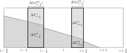
Figure 2: Illustration of the calculation of transported material volumes at each face. The filled regions show the reconstructed interface between two materials. The hatched regions denote the advected volumes, with widths given in terms of the interfacial speeds. The transported material volumes consist of the intersection of these regions with each material.

3.4 Mixed-cell update

The specialised mixed-cell update must be applied in all cells containing more than one material, but additionally in cells that could become mixed following the update. In practice this means all pure cells that are adjacent to a mixed-cell in the direction of the sweep, or two adjacent pure cells containing different materials (in the case where the material interface coincides exactly with the adjoining face). Even in the most demanding multi-material calculations this will typically be less than $10\%$ of the total cell count, so the computational burden of this process is small.

Following interface reconstruction, the intermediate volume fractions (neglecting contributions from the right-hand side of (10)) are computed using volume-of-fluid advection

$$\tilde{\phi}^{l}=\phi^{l,n}-\frac{\Delta V^{l}_{R}-\Delta V^{l}_{L}}{V}$$ (75)

where $V$ is the volume of the cell. In this section the subscripts $L$ and $R$ are used as short-hand for $i-\frac{1}{2}$ and $i+\frac{1}{2}$ respectively to denote quantities located at the left and right faces of the cell under consideration.

Following application of (75), the sum of the volume fractions $\tilde{\phi}^{l}$ in the cell may not equal one (whenever the velocity divergence is non-zero). The difference ($1-\sum_{m}\tilde{\phi}^{m}$) must be redistributed amongst the materials in the cell in accordance with their relative compressibility. To compute the right-hand side of (10) we require the bulk modulus for each material following advection, denoted $\tilde{K}_{S}^{l}$, which we obtain through a volume-weighted averaging procedure as detailed in [38, 12]

$$\tilde{K}^{l}_{S,i}=\frac{\Delta V^{l}_{L}\widehat{K}^{l}_{S,L}+\phi^{l}_{i}V_{i}K^{l}_{S,i}-\Delta V^{l}_{R}\widehat{K}^{l}_{S,R}}{\tilde{\phi}^{l}_{i}V_{i}}$$ (76)

where the upwind bulk moduli at the left and right faces are given by

$$\widehat{K}^{l}_{S,L} =\begin{cases}K^{l}_{S,i-1}\,&\text{if}\quad u^{\mathrm{int}}_{i-\frac{1}{2}}>0\\ K^{l}_{S,i}\,&\text{otherwise}\end{cases}$$ (77)

$$\widehat{K}^{l}_{S,R} =\begin{cases}K^{l}_{S,i}\,&\text{if}\quad u^{\mathrm{int}}_{i+\frac{1}{2}}>0\\ K^{l}_{S,i+1}\,&\text{otherwise}\end{cases}$$ (78)

The post-advection bulk modulus of the mixture is then

$$\widetilde{K}_{S}=\left(\sum_{l}\frac{\tilde{\phi}^{l}}{\tilde{K}^{l}_{S}}\right)^{-1}$$ (79)

Note that the same approach is used to determine the post-advection Grüneisen parameters $\tilde{\Gamma}^{l}$ and $\widetilde{\Gamma}$ used in the internal energy equations below. The final volume fractions are then given by

$$\phi^{l,n+1}=\tilde{\phi}^{l}+(1-\sum_{m}\tilde{\phi}^{m})\frac{\tilde{\phi}^{l}\widetilde{K}_{S}}{\tilde{K}_{S}^{l}}$$ (80)

where the bracketed expression may be identified as the time integral of the velocity divergence

$$(1-\sum_{m}\tilde{\phi}^{m})=\Delta t\frac{u_{R}^{\mathrm{int}}-u_{L}^{\mathrm{int}}}{\Delta x}$$ (81)

The mass, momentum and energy transported across the face of each mixed-cell are computed using upwinding. This is important to ensure that the procedure is self-consistent: when the cell is emptied of material $l$, the corresponding contributions to mass, momentum and energy must be set to zero. The relevant upwind quantities (denoted with a wide hat $\widehat{q}$) are calculated at the left and right faces of the cell as in (77) and (78) respectively. We also require the transported density of the mixture at each face, given by

$$\widehat{\rho}_{K}=\frac{\sum_{l}\widehat{\rho}^{l}_{K}\Delta V^{l}_{K}}{\sum_{l}\Delta V^{l}_{K}},\quad\mathrm{for}\>K=L,R$$ (82)

The discrete update equations for the partial densities, momenta, elastic stretches and history variables are as follows. The advective terms are differenced in line with (75). Note that the inelastic and history-rate source terms are omitted as these are evaluated separately.

$$\phi^{l,n+1}\rho^{l,n+1}= \;\phi^{l,n}\rho^{l,n}-\frac{\Delta V^{l}_{R}\widehat{\rho}^{l}_{R}-\Delta V^{l}_{L}\widehat{\rho}^{l}_{L}}{V}$$ (83)

$$\rho^{n+1}u^{n+1}_{i}= \;\rho^{n}u^{n}_{i}-\frac{\Delta V_{R}\widehat{\rho}_{R}\widehat{u}_{i,R}-\Delta V_{L}\widehat{\rho}_{L}\widehat{u}_{i,L}}{V}+\Delta t\frac{\sigma^{\mathrm{int}}_{i1,R}-\sigma^{\mathrm{int}}_{i1,L}}{\Delta x}$$ (84)

$$\overline{V}_{e,ij}^{n+1}= \;\overline{V}_{e,ij}^{n}-\frac{\Delta V_{R}\widehat{\overline{V}}_{e,ij,R}-\Delta V_{L}\widehat{\overline{V}}_{e,ij,L}}{V}+\frac{2}{3}\overline{V}_{e,ij}^{n}(1-\sum_{l}\tilde{\phi}^{l})\;+$$ (85)

$$\;\frac{\Delta t}{\Delta x}\left[(u^{n}_{j}-u^{\mathrm{int}}_{j,L})\overline{V}^{\mathrm{int}}_{e,1j,L}+(u^{\mathrm{int}}_{j,R}-u^{n}_{j})\overline{V}^{\mathrm{int}}_{e,1j,R}\right]$$

$$\phi^{l,n+1}\rho^{l,n+1}\pi^{l,n+1}_{m}= \;\phi^{l,n}\rho^{l,n}\pi^{l,n}_{m}-\frac{\Delta V^{l}_{R}\widehat{\rho}^{l}_{R}\widehat{\pi}^{l}_{m,R}-\Delta V^{l}_{L}\widehat{\rho}^{l}_{L}\widehat{\pi}^{l}_{m,L}}{V}$$ (86)

The momentum update (84) is importantly not the same as the one from [38], which used the interfacial velocity rather than the upwinded velocity in the advective terms. We found the original to be highly unstable when a dense material is leaving a cell containing a light material, as the dense material’s contribution to the momentum is not correctly set to zero. This resulted in large spikes in velocity which caused calculations to fail. The new update does not exhibit these problems.

The discrete energy update based on (25) is given by

$$\phi^{l,n+1}\rho^{l,n+1}\mathscr{E}^{l,n+1} =\,\phi^{l,n}\rho^{l,n}\mathscr{E}^{l,n}-\Delta_{\mathrm{adv}}-p^{l,\bigstar}\Delta_{\mathrm{vol}}+\Delta_{\mathrm{shear}}$$ (87)

$$\Delta_{\mathrm{adv}} =\frac{\Delta V^{l}_{R}\widehat{\rho}^{l}_{R}\widehat{\mathscr{E}}^{l}_{R}-\Delta V^{l}_{L}\widehat{\rho}^{l}_{L}\widehat{\mathscr{E}}^{l}_{L}}{V}$$

$$\Delta_{\mathrm{vol}} =(1-\sum_{m}\tilde{\phi}^{m})\frac{\tilde{\phi}^{l}\widetilde{\Gamma}}{\tilde{\Gamma}^{l}}$$

$$\Delta_{\mathrm{shear}} =2G^{l,\bigstar}\left[\sum_{i}\mathrm{dev}(\mathbf{H}_{e})^{\bigstar}_{i1}\Delta t\frac{u^{\mathrm{int}}_{i,R}-u^{\mathrm{int}}_{i,L}}{\Delta x}\right]\frac{\tilde{\phi}^{l}\widetilde{\Gamma}}{\tilde{\Gamma}^{l}}$$

Cutforth et al. presented an energy update which reportedly improved robustness significantly in complex simulations [12]. Following their approach, the time-level of the pressure $p^{l,\bigstar}$ in the discrete energy equation is taken to differ depending on whether the cell is in compression or expansion:

$$p^{l,\bigstar}=\begin{cases}p^{l,n}\,&\text{if}\quad u^{\mathrm{int}}_{R}-u^{\mathrm{int}}_{L}<0\\ p^{l,n+1}\,&\text{otherwise}\end{cases}$$ (88)

In order to ensure a consistent evaluation of the stress, the same logic is applied when chosing the time-level of the shear modulus $G^{l,\bigstar}$ and the deviatoric strain $\mathrm{dev}(\mathbf{H}_{e})^{\bigstar}$.

In the case of compression the update may be readily evaluated. In the implicit case (expansion), we invoke the equation of state (11) to rearrange the right-hand side

$$\phi^{l,n+1}\rho^{l,n+1}\mathscr{E}^{l,n+1}=\frac{\phi^{l,n}\rho^{l,n}\mathscr{E}^{l,n}-\Delta_{\mathrm{adv}}+\Delta_{\mathrm{vol}}(\rho^{l,n+1}\Gamma^{l,n+1}\mathscr{E}^{l,n+1}_{\mathrm{ref}}-p^{l,n+1}_{\mathrm{ref}})+\Delta_{\mathrm{shear}}}{1+\Delta_{\mathrm{vol}}\Gamma^{l,n+1}/\phi^{l,n+1}}$$ (89)

Then all of the variables on the right-hand side of (89) are known: $\phi^{l,n+1}$ is given by (80), $\rho^{l,n+1}$ is given by (83), $\mathrm{dev}(\mathbf{H}_{e})^{n+1}$ is given by (85), and $\Gamma^{l,n+1}$, $\mathscr{E}^{l,n+1}_{\mathrm{ref}}$, $p^{l,n+1}_{\mathrm{ref}}$ and $G^{l,n+1}$ are all assumed to depend only on $\rho^{l,n+1}$ and $\mathrm{dev}(\mathbf{H}_{e})^{n+1}$.

In the case of other equations of state where a closed-form rearrangement is not possible (for instance reactive mixtures along the lines of [55], or cavitating liquids along the lines of [59]), a root-finding procedure may be used to perform the implicit update.

3.5 Pressure relaxation

After the update mixed-cells will not in general be in pressure equilibrium, which is a requirement of the base diffuse-interface method. A pressure relaxation step is therefore included to iteratively adjust volume-fractions and internal energies until equilibrium is attained. We first outline the pressure relaxation scheme proposed by Miller and Puckett in [38], and then describe changes we have made to improve robustness.

The following equations are solved to adjust the component pressures in mixed-cells towards equilibrium in a controlled manner.

$$\overline{p}=p^{l}+\Delta p^{l} =p^{l}-\frac{K^{l}_{S}}{\phi^{l}}\Delta\phi^{l}$$ (90)

$$\sum_{l}\Delta\phi^{l} =0$$ (91)

These yield approximate expressions for the equilibrium pressure $\overline{p}$ and the required change in volume-fraction for each material $\Delta\phi^{l}$

$$\overline{p} =\frac{\sum_{l}\phi^{l}p^{l}/K^{l}_{S}}{\sum_{l}\phi^{l}/K^{l}_{S}}$$ (92)

$$\Delta\phi^{l} =\frac{\phi^{l}}{K^{l}_{S}}(p^{l}-\overline{p})$$ (93)

Due to the linearisation implicit in (93), Miller and Puckett enforced a limit on the maximum relative volume change in a single iteration of the relaxation, viz. $|\Delta\phi^{l}/\phi^{l}|\leq\delta$. When the cell is under compression $\delta=0.1$, and $\delta=0.05$ in expansion.

On each iteration, (92) is used to obtain an estimate of the equilibrium pressure, which is then used in (93) to calculate the amount by which each volume-fraction should change. If any of the values exceed the threshold, all of them are rescaled (this ensures that they continue to sum to zero)

$$\Delta\phi^{l}\leftarrow\Delta\phi^{l}\min_{l}\frac{\delta}{|\Delta\phi^{l}/\phi^{l}|}$$ (94)

Finally the volume-fractions are changed, and a $p\mathrm{d}v$ correction is made to each partial internal energy

$$\phi^{l} \leftarrow\phi^{l}+\Delta\phi^{l}$$ (95)

$$\rho^{l}\phi^{l}\mathscr{E}^{l} \leftarrow\rho^{l}\phi^{l}\mathscr{E}^{l}-\overline{p}\Delta\phi^{l}$$ (96)

The process is repeated until each component pressure is within some prescribed tolerance.

We found the above scheme to lack robustness, particularly within solids where tiny changes in volume-fraction result in relatively large changes in pressure. We observed oscillatory behaviour around the desired equilibrium point, where the calculated volume-fraction changes would repeatedly overshoot the target pressure, resulting in non-convergence. In order to address this we modify the threshold adaptively. Each time a sign-change is detected in $\Delta\phi^{l}$ we reduce the threshold value $\delta$. The threshold is given by

$$\delta=\delta_{0}\mathrm{exp}(-\alpha N_{\mathrm{sign}})$$ (97)

where $\delta_{0}$ is the initial threshold value, $\alpha$ is a free parameter that controls the rate of fall-off, and $N_{\mathrm{sign}}$ is the number of iterations in which a sign-change in $\Delta\phi^{l}$ has been detected. We typically take $\delta_{0}=0.01$ and $\alpha=0.1$. Unlike Miller and Puckett we do not distinguish between compression and expansion when applying the threshold.

3.6 Plastic update

The plastic source term $\boldsymbol{\Phi}$ is evaluated as detailed by Barton [5]. This update is independent of the volume-of-fluid method and is performed identically in pure and mixed cells, but is summarised here for completeness. First the following ordinary differential equation is solved using the backwards Euler method to evolve the strain invariant for each material that adheres to a plasticity law

$$\dot{\mathcal{J}}^{l}=-\sqrt{\frac{3}{2}}\chi^{l},\quad\mathcal{J}^{l,\bullet}\in[0,\mathcal{J}^{l,\circ}]$$ (98)

and the mixture strain invariant is obtained following

$$\mathcal{J}=\frac{\sum_{l}\phi^{l}\mathcal{J}^{l}/\Gamma^{l}}{\sum_{l}\phi^{l}/\Gamma^{l}}$$ (99)

where $\mathcal{J}^{l}\equiv 0$ in fluids. It is noted that since the ODE only need be solved for materials where $\phi^{l}>0$ the volume-of-fluid method increases the efficiency of this update by virtue of there being fewer mixed cells. Finally the mixture strain invariant at the new time level is used to update the stretch tensor

$$\overline{\mathbf{V}}^{\bullet}_{e}=\mathrm{exp}\left(\frac{\mathcal{J}^{\bullet}}{\mathcal{J}^{\circ}}\mathrm{dev}(\mathbf{H}^{\circ}_{e})\right)$$ (100)

In the course of this last step the symmetry and unimodularity of the stretch tensor is reinstated, which may be lost during the hyperbolic update:

$$\overline{\mathbf{V}}_{e}\leftarrow\sqrt{\overline{\mathbf{V}}_{e}\overline{\mathbf{V}}_{e}^{T}}$$ (101)

4 Verification and validation

4.1 Solid-solid Riemann problem

The first test is a solid-solid Riemann problem taken from [8], involving an interaction between aluminium and copper resulting in a complex wave structure. The initial left and right states are as follows:

$$\mathbf{u}_{L} =\begin{pmatrix}2\\ 0\\ 0.1\\ \end{pmatrix}\mathrm{km\,s}^{-1},\quad\mathbf{F}_{e,L}=\begin{pmatrix}1&0&0\\ -0.01&0.95&0.02\\ -0.015&0&0.9\\ \end{pmatrix},\quad\mathscr{E}_{L}=\mathscr{E}_{\mathrm{ref},L}$$

$$\mathbf{u}_{R} =\begin{pmatrix}0\\ -0.03\\ -0.01\\ \end{pmatrix}\mathrm{km\,s}^{-1},\quad\mathbf{F}_{e,R}=\begin{pmatrix}1&0&0\\ 0.015&0.95&0\\ -0.01&0&0.9\\ \end{pmatrix},\quad\mathscr{E}_{R}=\mathscr{E}_{\mathrm{ref},R}$$

where $\mathbf{F}_{e}$ is the elastic deformation gradient tensor, from which the initial densities and elastic stretches are found via

$$\rho =\frac{\rho_{0}}{\mathrm{det}|\mathbf{F}_{e}|}$$ (102)

$$\overline{\mathbf{V}}_{e} =\frac{\sqrt{\mathbf{F}_{e}\mathbf{F}^{T}_{e}}}{\sqrt[3]{\mathrm{det}|\mathbf{F}_{e}|}}$$ (103)

Both materials are assumed to be purely elastic and are governed by the equation of state from [13] with parameters given in Table 1. The domain is $x\in[0,1]$ with the discontinuity initially located at $x=0.5$, with aluminium to the left and copper to the right. The problem is run to time $0.5\,\mu\mathrm{s}$ with CFL number 0.1.

Material	$\rho_{0}$ (g cm-3)	$K_{0}$ (GPa)	$G_{0}$ (GPa)	$\Gamma_{0}$	$\alpha$	$\beta$
Aluminium 6061-T6	2.703	76.3	26.36	1.484	0.627	2.288
Copper	8.930	136.45	39.38	2.0	1.0	3.0
Clay	1.932	49.4	6.0	1.0	1.0	-

Table 1: Material parameters for the equation of state from [13], as given in Section 2.4. Where $\beta$ is not specified a constant shear modulus is used: $G=G_{0}$.

Results are presented in Figure 4 for a mesh with 500 cells. The volume-of-fluid method (labelled VOF) is compared against the base diffuse-interface method with THINC interface sharpening [5] (labelled DI+THINC) and the exact solution derived using the method from [8]. Convergence is illustrated in Figure 5, which gives $L_{1}$-norms for density and velocity relative to the exact solution.

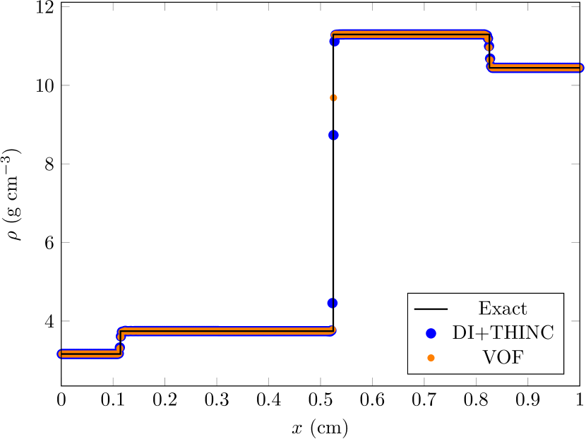
(a)

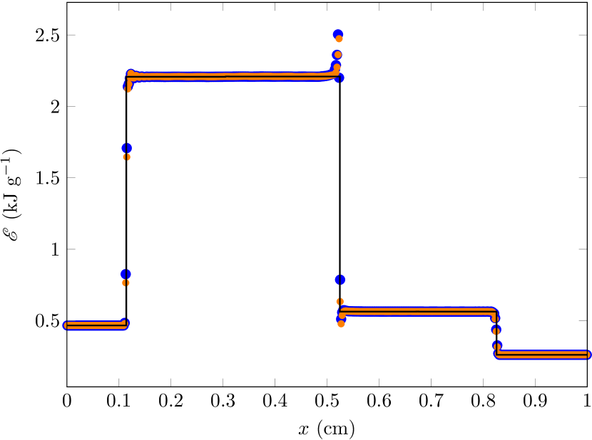
(b)

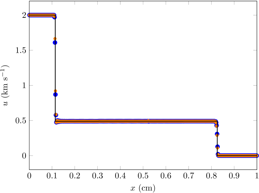
(c)

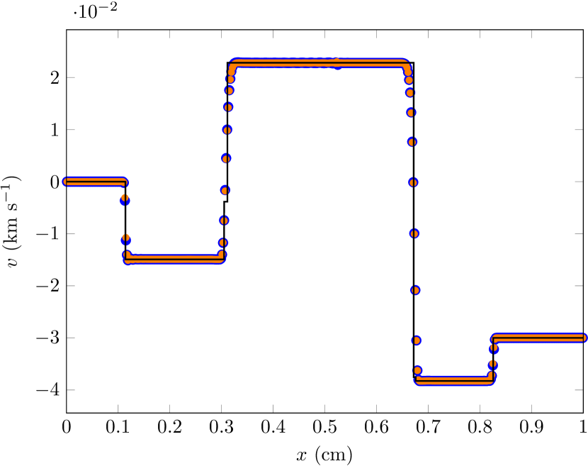
(d)

Figure 3: Solid-solid Riemann problem.

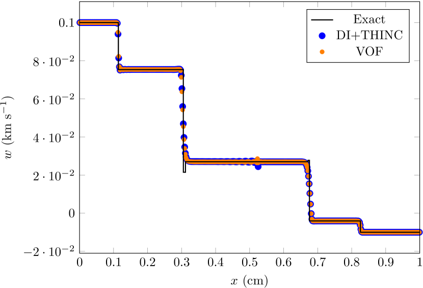
(a)

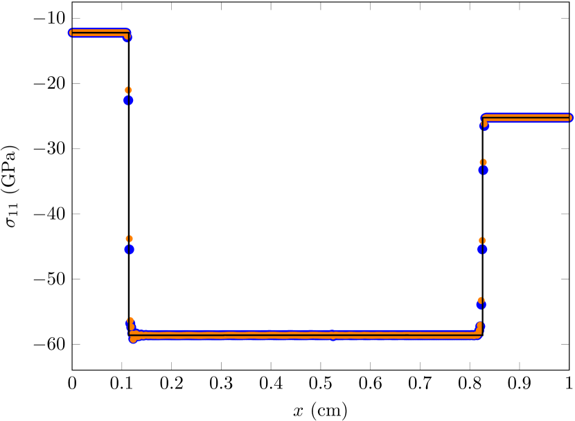
(b)

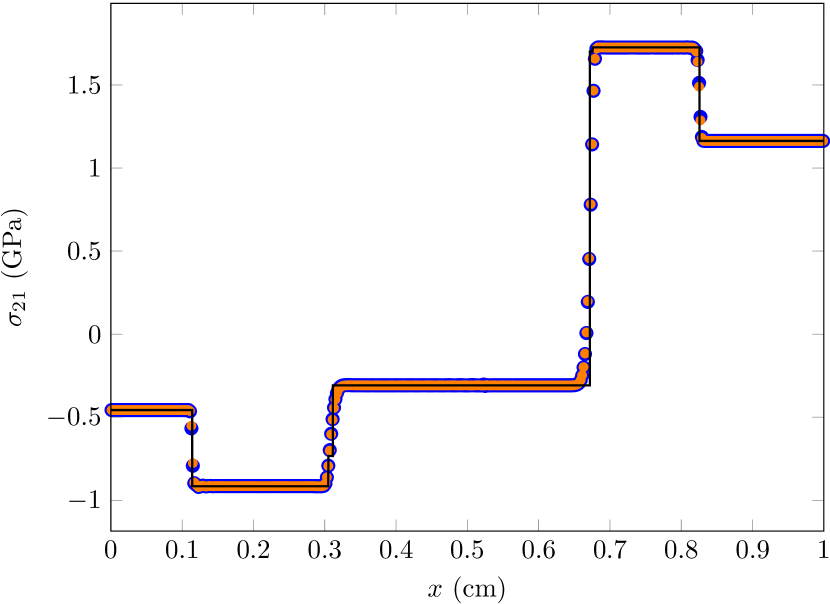
(c)

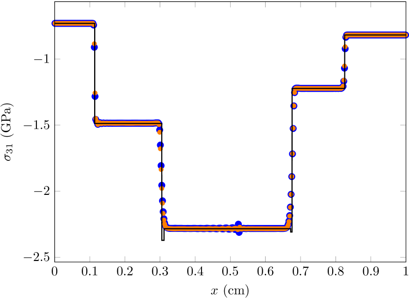
(d)

Figure 4: Solid-solid Riemann problem (cont.)

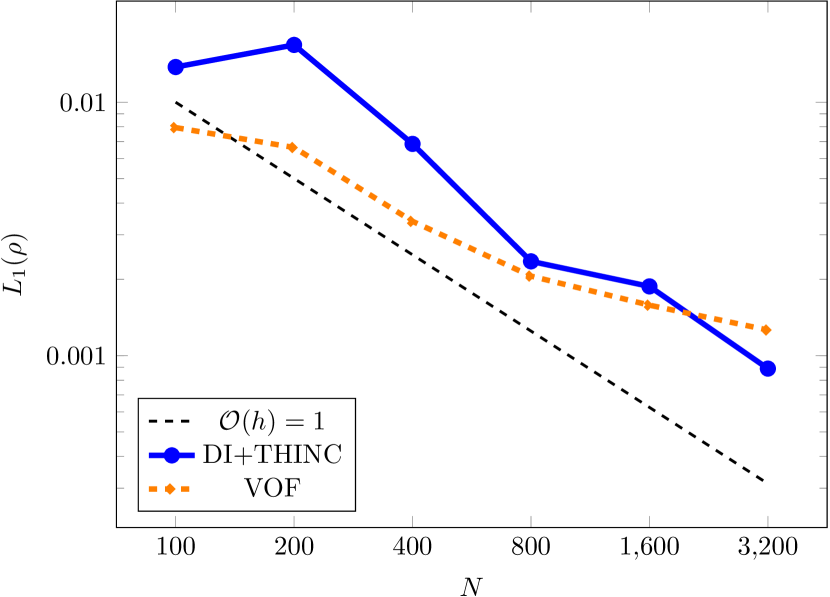
(a)

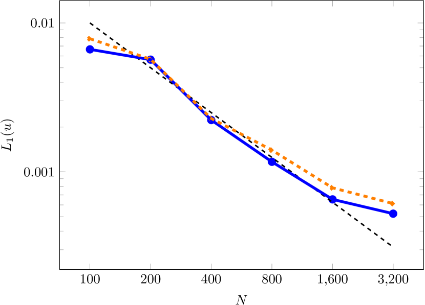
(b)

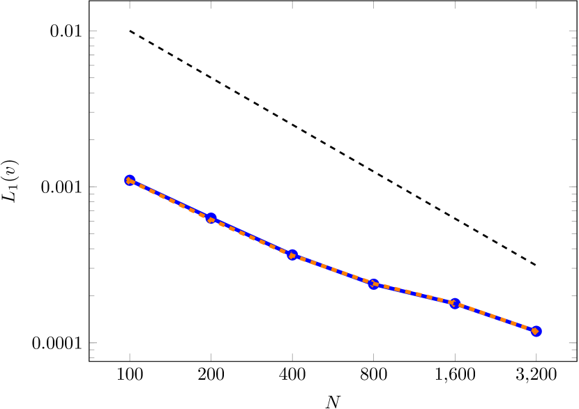
(c)

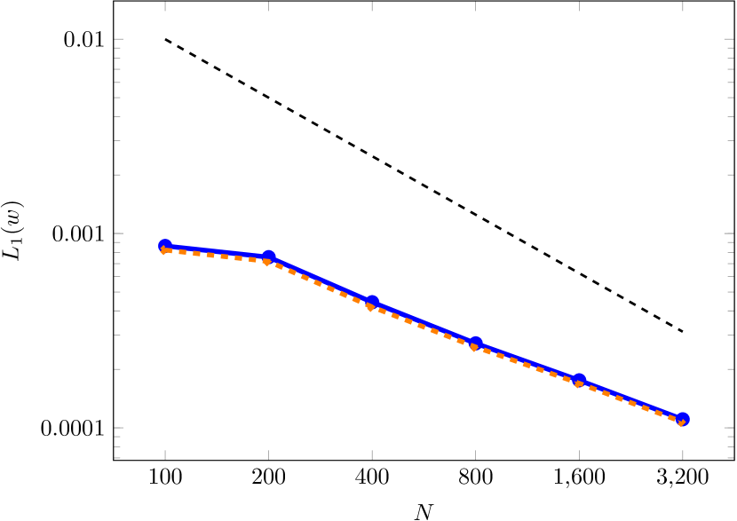
(d)

Figure 5: Solid-solid Riemann problem, $L_{1}$-norms versus exact solution.

As expected, away from the material interface the results are equivalent to the diffuse-interface solution, however at the contact the ability of the volume-of-fluid scheme to maintain a sharp interface is demonstrated. Barton noted that THINC contributes to oscillations in the tangential stress and velocity fields at the interface—these are notably reduced with the new method.

4.2 Solid-fluid Riemann problem

The second test is a solid-fluid Riemann problem, again taken from [8], featuring highly stressed moving aluminium in contact with quiescent air. This test is used to verify that the volume-of-fluid method can correctly treat an interface between two materials with radically different properties. The initial left and right states are as follows:

$$\mathbf{u}_{L} =\begin{pmatrix}2\\ 0\\ 0.1\\ \end{pmatrix}\mathrm{km\,s}^{-1},\quad\mathbf{F}_{e,L}=\begin{pmatrix}1&0&0\\ -0.01&0.95&0.02\\ -0.015&0&0.9\\ \end{pmatrix},\quad\mathscr{E}_{L}=\mathscr{E}_{\mathrm{ref},L}$$

$$\mathbf{u}_{R} =\mathbf{0}\>\mathrm{km\,s}^{-1},\quad\overline{\mathbf{V}}_{e,R}=\mathbf{I},\quad\rho_{R}=10^{-3}\>\mathrm{g\,cm}^{-3},\quad p_{R}=10^{-4}\>\mathrm{GPa}$$

The aluminium is assumed to be purely elastic and is governed by the equation of state from [13] with parameters given in Table 1. The air is governed by an ideal gas equation of state with $\gamma=1.4$. The problem is run to time $0.6\,\mu\mathrm{s}$ with CFL number 0.1.

Results are shown in Figure 6. The exact solution has been computed for the case with vacuum instead of air, but this makes little difference to the solution within the metal which is shown. The air supports a right-going shock not present in the vacuum which can be seen in the normal velocity field.

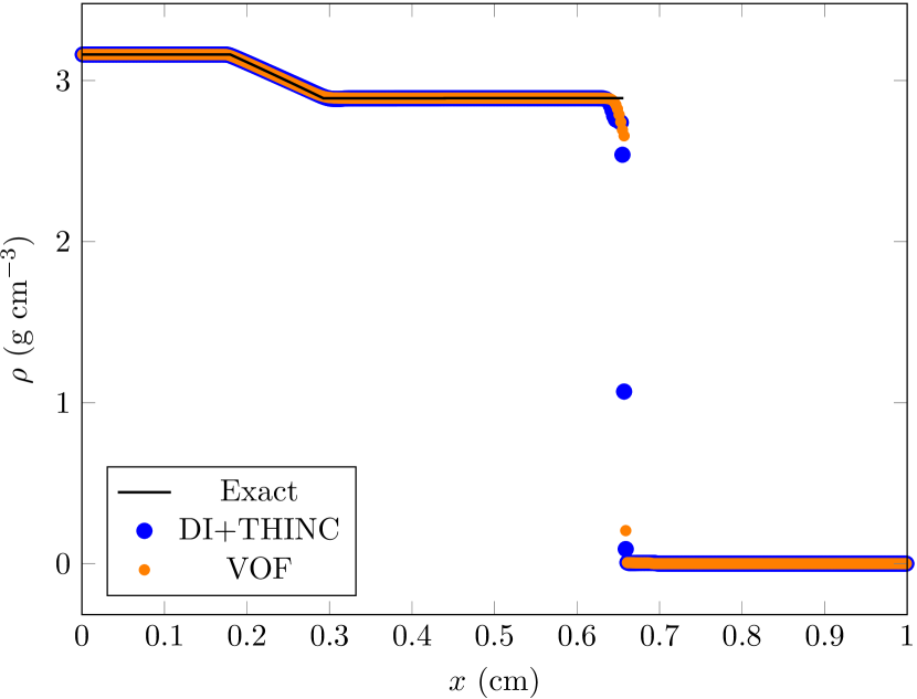
(a)

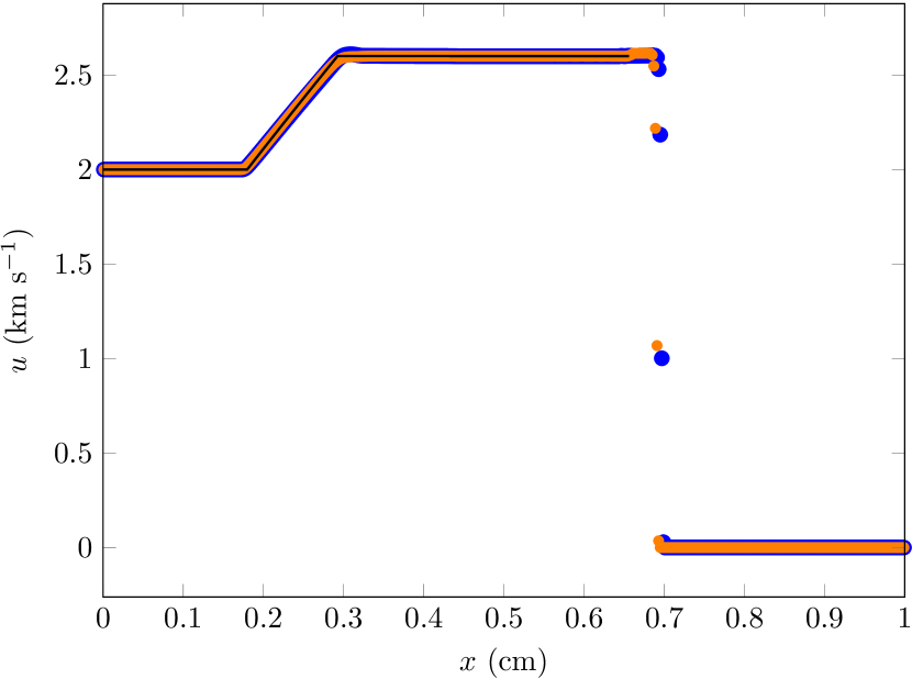
(b)

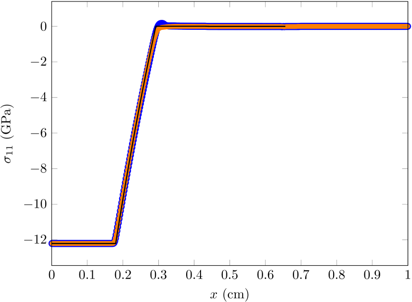
(c)

Figure 6: Solid-fluid Riemann problem.

4.3 Shell collapse

The shell collapse problem has been studied by many authors, an early contributor being Verney [54], and is a demanding test of energy conservation and symmetry preservation. This can be seen in solutions obtained using alternative Eulerian sharp interface treatments such as the ghost-fluid method, where high resolution is typically required to obtain a reasonable solution [6, 32]. In contrast our method exhibits smaller conservation errors and is able to provide excellent results even on extremely coarse meshes.

A cylindrical aluminium shell is modelled with initial inner radius of $0.8\,\mathrm{cm}$ and initial outer radius $1.0\,\mathrm{cm}$; the domain size is $[0,1.1]^{2}\,\mathrm{cm}$. An initial velocity distribution is applied that causes the shell to collapse incompressibly. Plastic distortional effects convert kinetic energy to internal energy, and eventually the shell stops. Howell and Ball present formulae for the stopping radii [20]. In this case we have a final inner radius of $0.3\,\mathrm{cm}$ and a final outer radius of approximately $0.671\,\mathrm{cm}$. The initial radial velocity is given by $0.8u_{0}/r$ where $u_{0}=0.437\,\mathrm{km\,s}^{-1}$. The equation of state parameters for the aluminium are given in Table 1, and ideal plasticity is used with constant yield stress $\sigma_{Y}=0.2976\,\mathrm{GPa}$. The remainder of the domain is filled with air governed by an ideal gas equation of state with $\gamma=1.4$ and $\rho_{0}=1.225\cdot 10^{-3}\,\mathrm{g\,cm}^{-3}$. The problem is run to time $30\,\mu\mathrm{s}$ with CFL number 0.6. Figure 7 shows snapshots of velocity magnitude within the shell, and the location of the interface, at $t=0$, $10$, $20$ and $30\,\mu\mathrm{s}$.

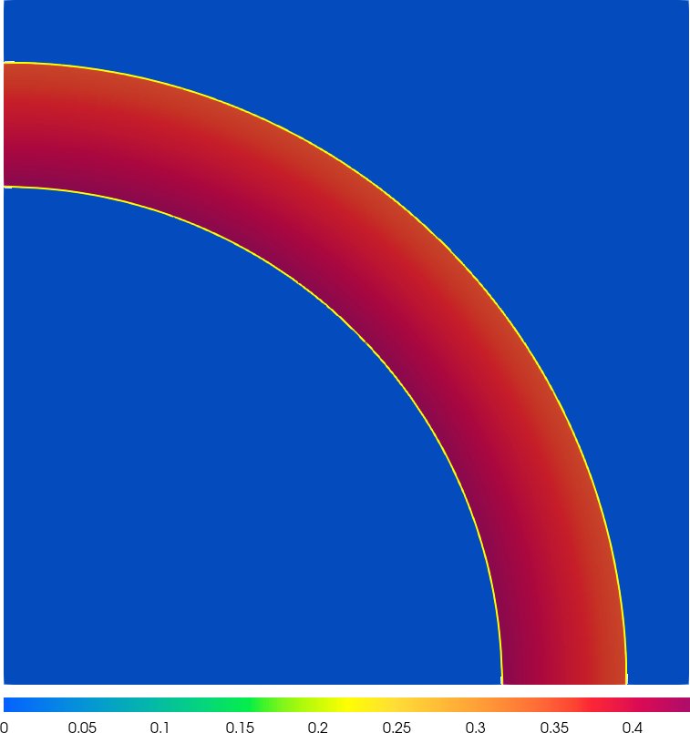
(a)

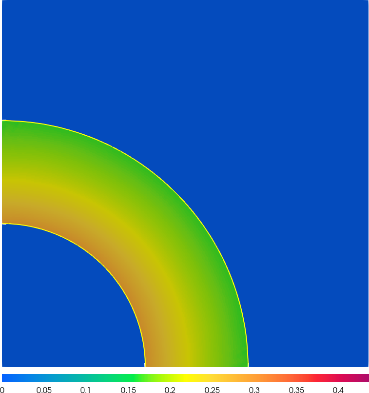
(b)

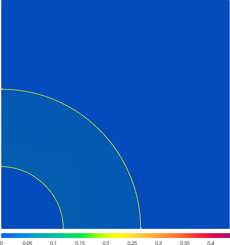
(c)

(d)

Figure 7: The collapsing shell problem: magnitude of velocity within the shell measured in $\mathrm{km\,s}^{-1}$ (velocity of surrounding air not shown) and $\phi=0.5$ contour at intervals of $10\,\mu\mathrm{s}$ from $t=0\,\mu\mathrm{s}$ to $t=30\,\mu\mathrm{s}$.

The final inner and outer radii are shown as a function of angle in Figure 8(a) and 8(b) respectively for a range of mesh sizes. In all cases it can be seen that the radial error is limited to less than $2\%$, even on a very coarse mesh with only 64 cells in each coordinate direction. In contrast, both Barton et al. [6] and Lopez Ortega et al. [32] report errors in the region of $35\%$ for similarly sized meshes using ghost-fluid methods. At higher (but still moderate) resolutions, the deviations from radial symmetry are reduced.

Conservation histories for total mass and total energy as shown in Figure 8(c) and 8(d) respectively for the same range of mesh sizes. Although the volume-of-fluid method is not fully conservative, it can be seen that the error in total mass for this problem is less than a fifth of a percent, and the error for total energy is limited to less than five percent.

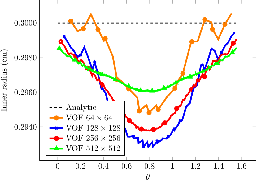
(a)

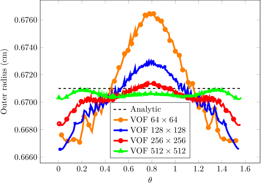
(b)

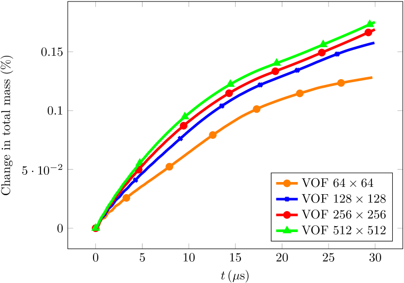
(c)

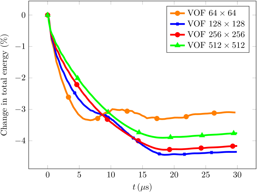
(d)

Figure 8: Final radii and energy conservation for the aluminium shell collapse problem at a range of mesh sizes. (a) shows the predicted inner radius as a function of the angle $\theta\in[0,\frac{\pi}{2}]$, (b) shows the predicted outer radius, (c) shows percentage conservation of total mass and (d) shows percentage conservation of total energy. The dashed lines show the analytic radii computed using the formulae from Howell and Ball [20]. The volume-of-fluid method produces excellent results even at the coarsest mesh resolution, in stark contrast to previously published ghost-fluid method results. Radial symmetry is well preserved and improves as the mesh is refined, and conservation errors are low.

4.4 Cylinder impact

Cylinder impacts provide a strenuous test of elasto-plastic flow and are included here to validate the rate-sensitive plasticity treatment. A cylinder strikes a rigid anvil (here modelled using a perfectly reflecting boundary) and deforms plastically, flowing radially outwards until all kinetic energy has been converted to internal energy and the cylinder stops, with a reduced length. Wilkins and Guinan provide experimental data in [58], and we also compare against results given by Barton [5] using the underlying diffuse-interface method.

The initial length of the cylinder is $L_{0}=2.347\,\mathrm{cm}$ and the radius is $0.381\,\mathrm{cm}$. We predict the final length $L_{f}$ for a range of impact velocities in 2D axisymmetric geometry, using a domain of $1.25\times 2.5\,\mathrm{cm}$ and a mesh size of $512\times 1024$. The cylinder is aluminium 6061-T6 with parameters given in Table 1. The Johnson-Cook rate-sensitive plasticity model is used, including work-hardening effects, with parameters given in Table 2. Thermal softening is disabled here by setting $T_{\mathrm{melt}}\rightarrow\infty$. The cylinder is immersed in quiescent air governed by an ideal gas equation of state with $\gamma=1.4$ and $\rho_{0}=1.225\cdot 10^{-3}\,\mathrm{g\,cm}^{-3}$. All materials are initialised to a pressure of $1\,\mathrm{atm}$ and a CFL number of 0.6 is used. The time evolution of the cylinder/air interface and the equivalent plastic strain is shown for the $373\,\mathrm{m\,s}^{-1}$ case in Figure 9.

Material	$c_{1}$	$c_{2}$	$c_{3}$	$n$	$\chi_{0}$	$m$	$T_{0}\,(\mathrm{K})$	$T_{\mathrm{melt}}\,(\mathrm{K})$
Aluminium 6061-T6	0.324	0.114	0.002	0.45	$10^{-5}$	-	-	-
Copper	0.09	0.292	0.025	0.31	$10^{-5}$	1.09	288.15	1356

Table 2: Parameters for the Johnson-Cook rate-sensitive plasticity model.

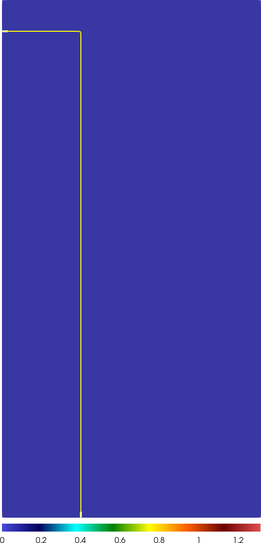
(a)

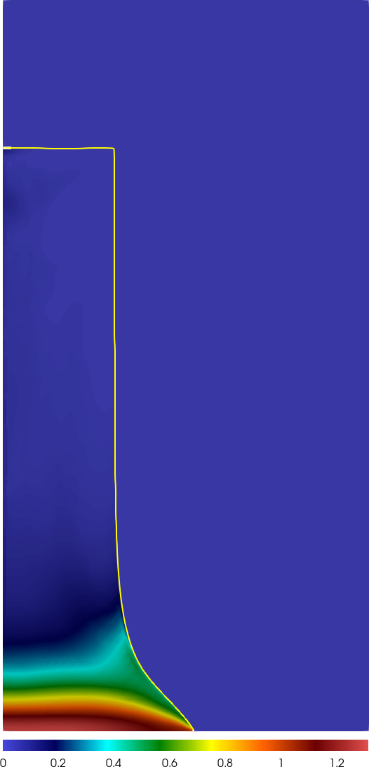
(b)

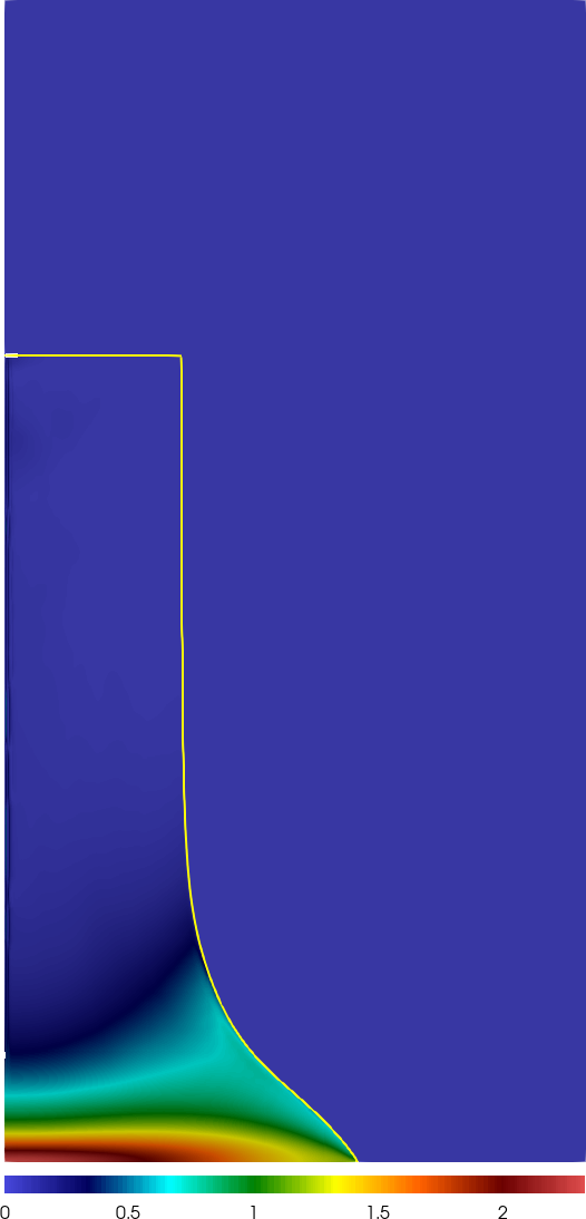
(c)

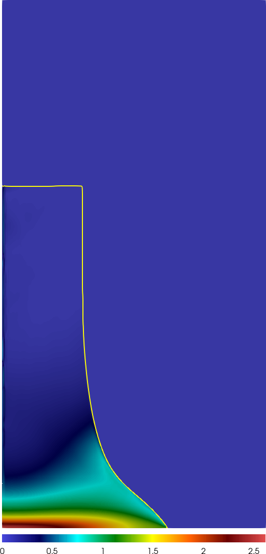
(d)

Figure 9: The cylinder impact problem with an impact velocity of $373\,\mathrm{m\,s}^{-1}$: equivalent plastic strain is shown along with the $\phi=0.5$ contour at intervals of $10\,\mu\mathrm{s}$ from $t=0\,\mu\mathrm{s}$ to $t=30\,\mu\mathrm{s}$.

The final ratios $L_{f}/L_{0}$ for each impact velocity are compared in Figure 10. The volume-of-fluid method matches experiment very well, correctly predicting the non-linear trend.

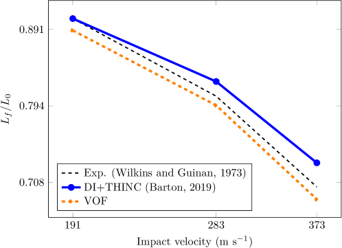
Figure 10: Results for the cylinder impact test case. The ratio of the final length of the cylinder to its initial length, both from experiment and predicted using the DI+THINC and VOF methods.

4.5 Buried explosive

The buried explosive problem previously studied in [5] is useful to contrast the behaviour of the volume-of-fluid method against the diffuse-interface method for problems involving large deformations and interface breakup. A charge buried in soft clay detonates resulting in ejecta and crater formation.

For 2D axisymmetric simulations the domain is $[0,2]\times[-2,4]\,\mathrm{m}$. For full 3D simulations, one quadrant is modelled, and the domain is $[0,2]\times[-2,2]\times[0,2]\,\mathrm{m}$. The initial location of the clay/air interface is $y=0$. The material parameters for the clay are given in Table 1. Rather than using a fixed Grüneisen parameter, a power-law form is used

$$\Gamma=\Gamma_{0}\left(\frac{\rho}{\rho_{0}}\right)^{q}$$ (104)

with $q=1$. The air is modelled using an ideal gas equation of state with $\gamma=1.4$ and $\rho_{0}=1.225\cdot 10^{-3}\,\mathrm{g\,cm}^{-3}$. The clay and air are given an initial pressure of $1\,\mathrm{atm}$. The explosive products are initialised in the cylinder centred at $(0,-13.081,0)\,\mathrm{cm}$ with radius $8.763\,\mathrm{cm}$ and height $5.842\,\mathrm{cm}$. The phenomenological balloon model is used to model the explosive products, sharing the equation of state with the air [28]. The initial product density is $1.63\,\mathrm{g\,cm}^{-3}$, and the initial specific internal energy is $6.0568\,\mathrm{kJ\,g}^{-1}$. Gravitational and atmospheric effects are not important over the short timescales considered and so are not included.

Results for the 2D axisymmetric case are shown in Figure 11. Snapshots of pressure and a numerical Schlieren of density are shown at $t=0.3$, $1$, $1.8$ and $3\,\mathrm{ms}$ for the volume-of-fluid method and the underlying diffuse-interface method with THINC interface sharpening. The function used to define the Schlieren plots is from [43]

$$\mathrm{exp}\left(-\kappa\frac{|\nabla\rho|}{\underset{ijk}{\mathrm{max}}\,|\nabla\rho_{ijk}|}\right)$$

where we take $\kappa=8000$. At the earlier times, excellent agreement is seen between the two methods in terms of cavity dimensions and ground shock propagation. At the later times, the crater dimensions agree well and the volume-of-fluid method shows its strengths by resolving fine-scale turbulent structures resulting from the break up of the lofted clay, which are suppressed in the diffuse-interface solution. A zoomed in density Schlieren at the final time is shown in Figure 12(a) that highlights these details. Closer examination of the log-scale volume-fraction field in Figure 12(b) shows that the interface does not fully break when using the diffuse-interface method, instead unphysical thin ligaments with low but non-zero volume fraction develop.

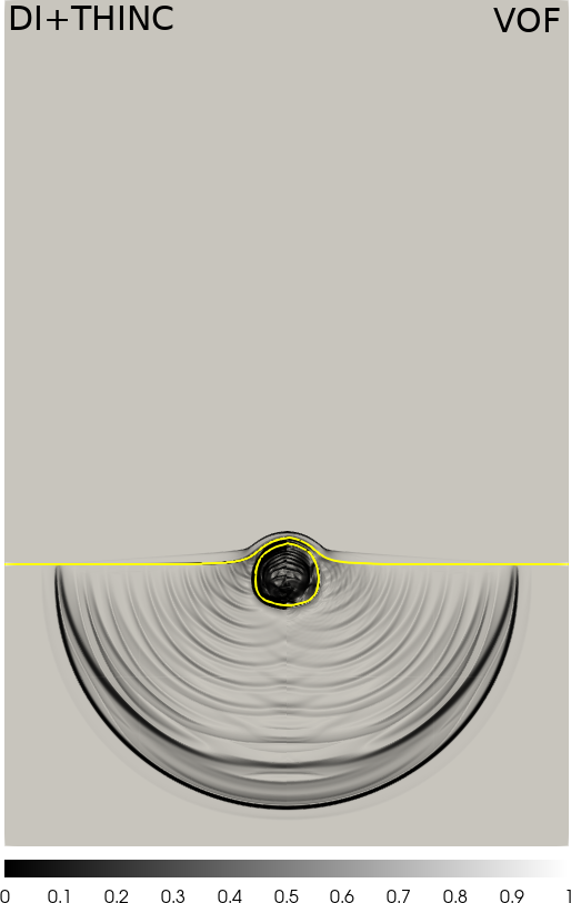
(a)

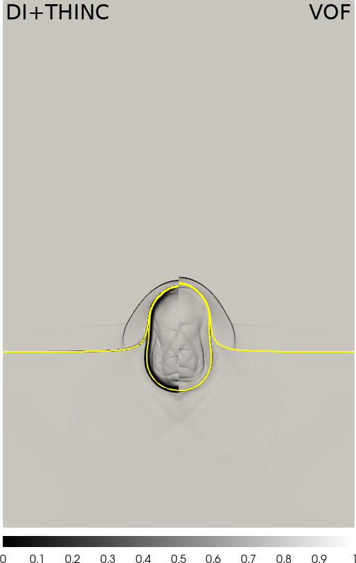
(b)

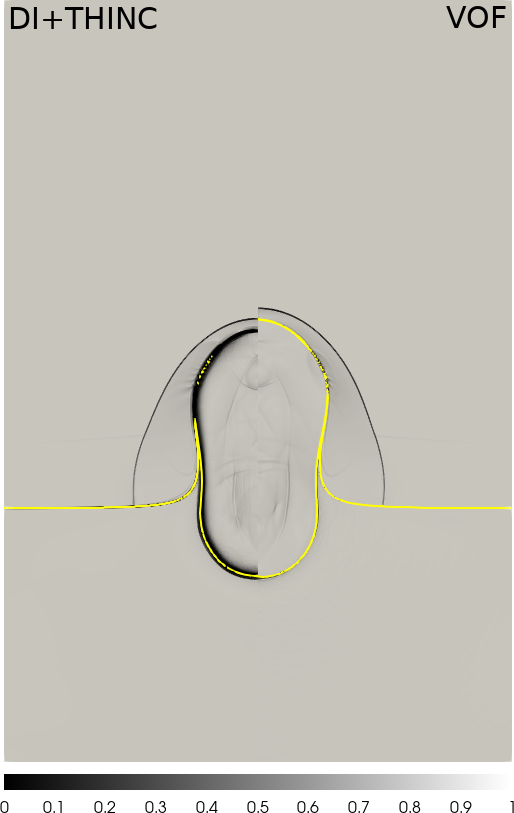
(c)

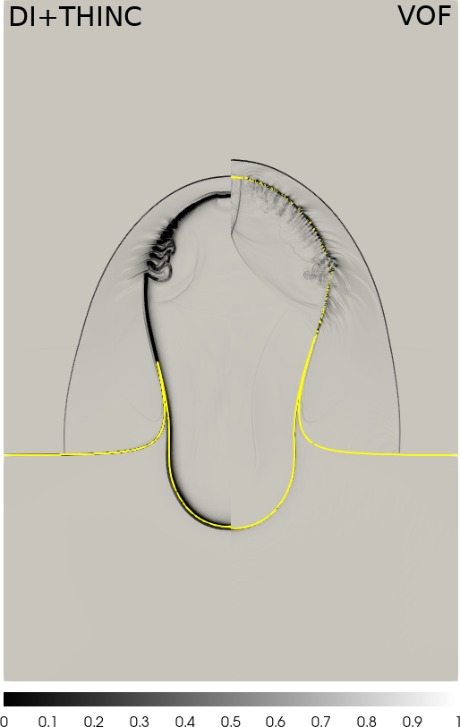
(d)

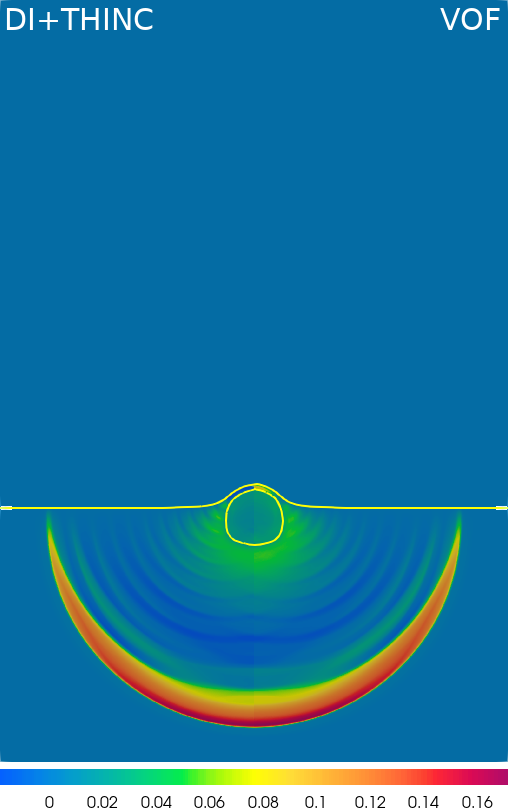
(e)

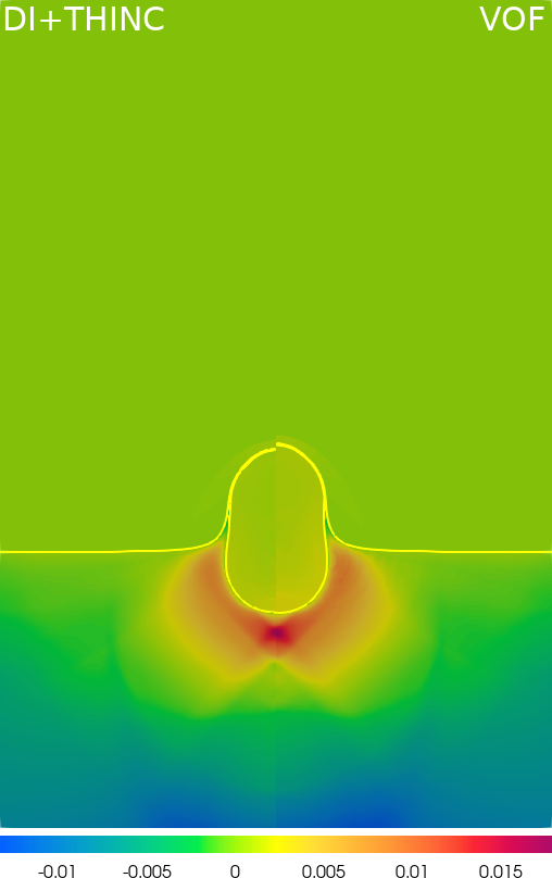
(f)

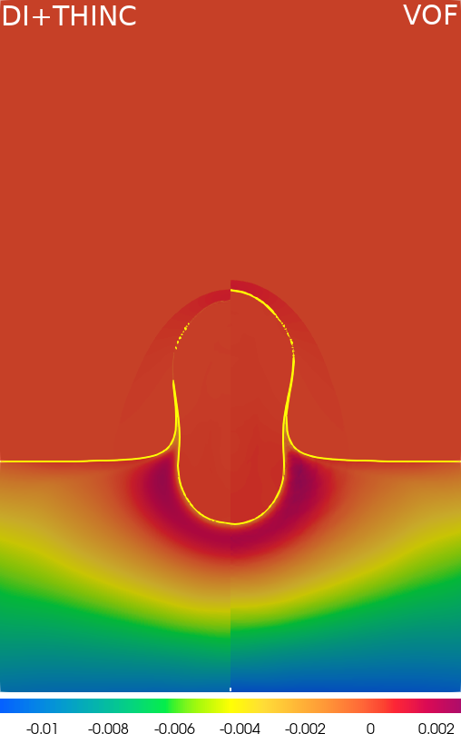
(g)

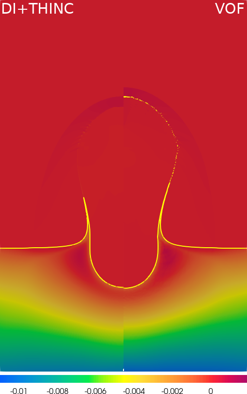
(h)

Figure 11: Comparison between DI+THINC and VOF for the 2D axisymmetric buried explosive problem. The mesh size is $800\times 2400$. Panels (a), (b), (c) and (d) show $t=0.3$, $1.0$, $1.8$ and $3\,\mathrm{ms}$ respectively, and similarly for panels (e)–(h). In each panel the left half of the image shows DI+THINC and the right half shows the corresponding VOF solution. The first row shows a numerical Schlieren of density and the second shows pressure measured in $\mathrm{GPa}$. The yellow lines denote the $\phi=0.5$ contour. While the two methods agree well on ground shock and crater dimensions, it is clear that the DI+THINC method has suppressed the growth of turbulent instabilities in the wake of lofted ejecta, which are much more pronounced in the VOF solution.

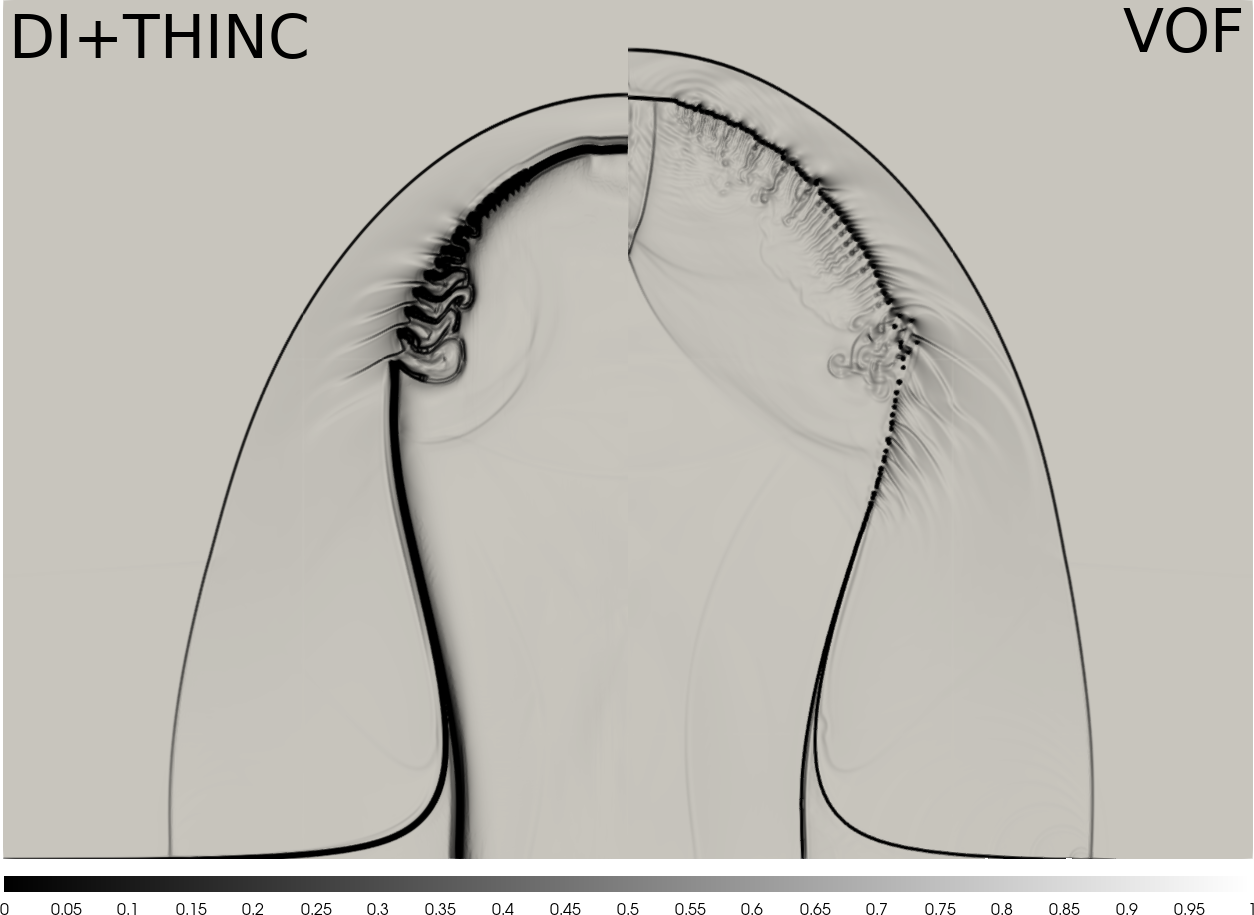
(a)

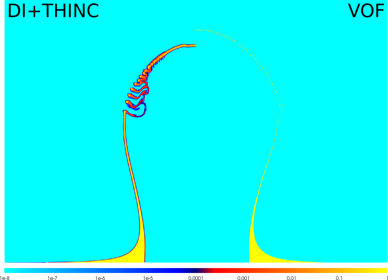
(b)

Figure 12: Close-up of $t=3\,\mathrm{ms}$ for the 2D axisymmetric buried explosion problem. (a) shows the numerical Schlieren of density, showing how the VOF method captures fine-scale turbulent flow in the wake of the lofted ejecta. (b) compares the log-scale clay ejecta volume fraction fields between DI+THINC and VOF. Unphysical ligament formation can be clearly observed in the DI+THINC solution, the interface never truly breaks. This is absent in the VOF solution.

Results from the 3D simulations are shown in Figure 13 including the contours of the clay/air interface and the pressure in the ground. Our findings are analogous to the 2D axisymmetric case, with good agreement between the two methods on cavity and crater dimensions, as well as ground shock propagation. The 3D volume-of-fluid method exhibits the same advantages as in 2D, showing excellent fidelity in the break-up of the lofted clay.

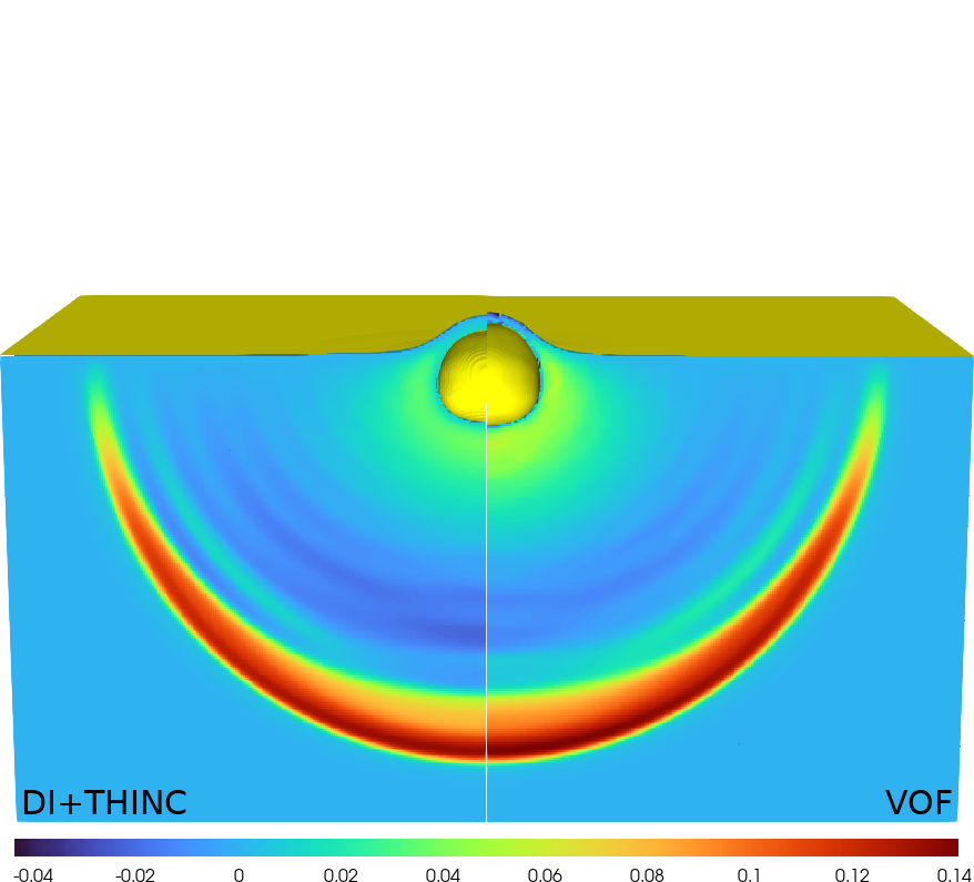
(a)

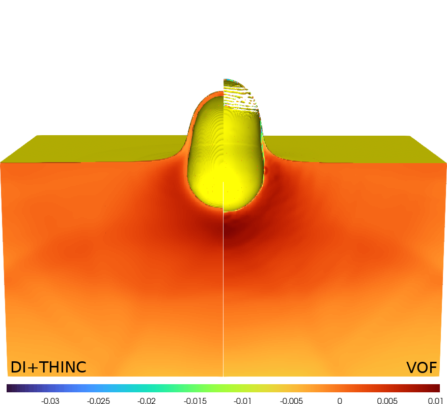
(b)

(c)

(d)

Figure 13: Comparison between DI+THINC and VOF for the 3D buried explosive problem. The mesh size is $240\times 480\times 240$. (a)–(d) show $t=0.3$, $1.0$, $1.4$ and $1.8\,\mathrm{ms}$ respectively. In each image the left half shows DI+THINC and the right half shows the corresponding VOF solution. The yellow contour shows the clay/air interface and the colouring indicates pressure. As in 2D the two methods agree well on ground shock and crater dimensions, but VOF offers much improved fidelity for the lofted ejecta.

5 Application: modelling the BRL 105mm shaped charge

In this section we apply the method to modelling the BRL $105\,\mathrm{mm}$ unconfined shaped charge as detailed in [2]. Shaped charges use convergent detonation waves in a high-explosive to produce a hyper-velocity metal jet with many industrial and defence applications. They are also stringent tests of elasto-plastic hydrodynamics methods as they typically include multiple materials arranged in a complex configuration and subject to extreme deformation. This particular shaped charge has been modelled by other authors [57, 3], allowing us to draw useful comparisons. Note that it is not our intention to fine tune the model to match experiment, only to show that the volume-of-fluid method is capable of treating this extremely strenuous scenario and producing reasonable results. It is noted that the underlying diffuse-interface method with THINC interface sharpening does not work well for this problem as the thin jet becomes smeared over a large area.

The 2D axisymmetric domain is $[0,6]\times[-6,40]\,\mathrm{cm}$, with the origin chosen to be coincident with the inner liner apex. The geometry of the shaped charge is given in [2], but unfortunately not all pertinent details are specified. For simplicity we omit the tetryl booster pellet and detonator from our model and ignore the rounded apex of the liner. Our modified geometry is shown in Figure 14.

Figure 14: The BRL 105mm unconfined shaped charge, simplified from the diagram given in [2].

The liner is copper with parameters given in Table 1. The Johnson-Cook rate-sensitive plasticity model is used, including both work-hardening and thermal-softening effects, with parameters given in Table 2. The high-explosive (Comp-B) is treated using the reactive burn model from [55], summarised in Section 2.4. The reactants and products both obey the JWL equation of state, with parameters given in Table 3. The explosive is assumed to have no strength hence $G=0$. The parameters for the ignition and growth model are $a=0.01$, $b=0.222$, $c=0.222$, $d=0.666$, $e=0.0$, $g=0.0$, $x=4.0$, $y=2.0$, $z=0.0$, $F_{ig}=0.3$, $F_{G_{1}}=1.0$, $F_{G_{2}}=1.0$, $I=4.4\cdot{}10^{2}\,(10\mu\mathrm{s})^{-1}$, $G_{1}=4.14\cdot{}10^{-1}\,\mathrm{GPa}^{-y}(10\mu\mathrm{s})^{-1}$ and $G_{2}=0.0\,\mathrm{GPa}^{-z}(10\mu\mathrm{s})^{-1}$, taken from [39]. The heat of detonation associated with the Comp-B is $6.3\,\mathrm{kJ\,g}^{-1}$. The shaped charge is immersed in air governed by an ideal gas equation of state with $\gamma=1.4$ and $\rho_{0}=1.225\cdot{}10^{-3}\,\mathrm{g\,cm}^{-3}$.

Comp-B	$\rho_{0}$ (g cm-3)	$A$ (GPa)	$B$ (GPa)	$R_{1}$	$R_{2}$	$\Gamma_{0}$	$C_{V}$ (kJ K-1 g-1)
Reactants	$1.717$	$7.781\cdot{}10^{4}$	$-5.031$	$11.3$	$1.13$	$0.8938$	$2.487\cdot{}10^{-3}$
Products	$1.717$	$5.242\cdot{}10^{2}$	$7.678$	$4.2$	$1.1$	$0.34$	$10^{-3}$

Table 3: JWL equation of state parameters for Comp-B, taken from [39].

All materials are initialised to a pressure of $1\,\mathrm{atm}$, except for a hemispherical booster region centred at the back of the explosive with radius $1.439\,\mathrm{cm}$ and pressure $27\,\mathrm{GPa}$, used to initiate the detonation. Twenty five Lagrangian tracer particles are initially located along the inner surface of the liner, evenly spaced along the $z$-axis at intervals of $0.25\,\mathrm{cm}$ starting from $z=3.0\,\mathrm{cm}$. The time history of the velocity is measured for each tracer particle.

Figure 15(a)–15(d) shows the high-explosive burn and subsequent collapse of the liner that occurs during the first eighteen microseconds. The detonation wave is initiated by the high pressure booster region. Just after $t=3\,\mu\mathrm{s}$ the wave strikes the apex of the liner and pressure begins to build up in that region. At $t=12\,\mu\mathrm{s}$ the jet is beginning to form as the liner turns in and is rapidly accelerated. By $t=18\,\mu\mathrm{s}$ the high-explosive is fully burnt and the high pressure stagnant region can be clearly seen. Figure 15(e) and 15(f) show the late-time jet formation at $t=45$ and $60\,\mu\mathrm{s}$ respectively. The jet reaches a stable speed and begins to thin out due to the velocity gradient along its length. The jet also has a blunt tip, which is in good agreement with the Arbitrary Lagrangian-Eulerian results presented by Barlow et al. [3], and as they note matches what is typically seen in experiment. Close inspection of the density field reveals fragments of copper breaking off the tip.

(a)

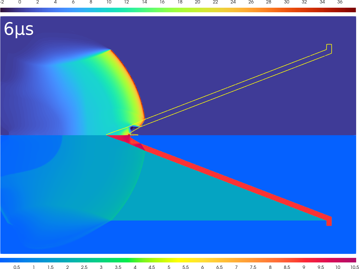
(b)

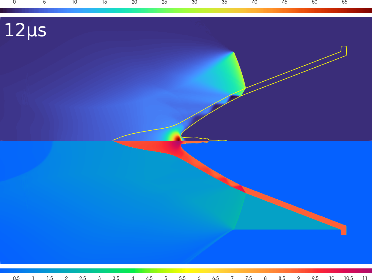
(c)

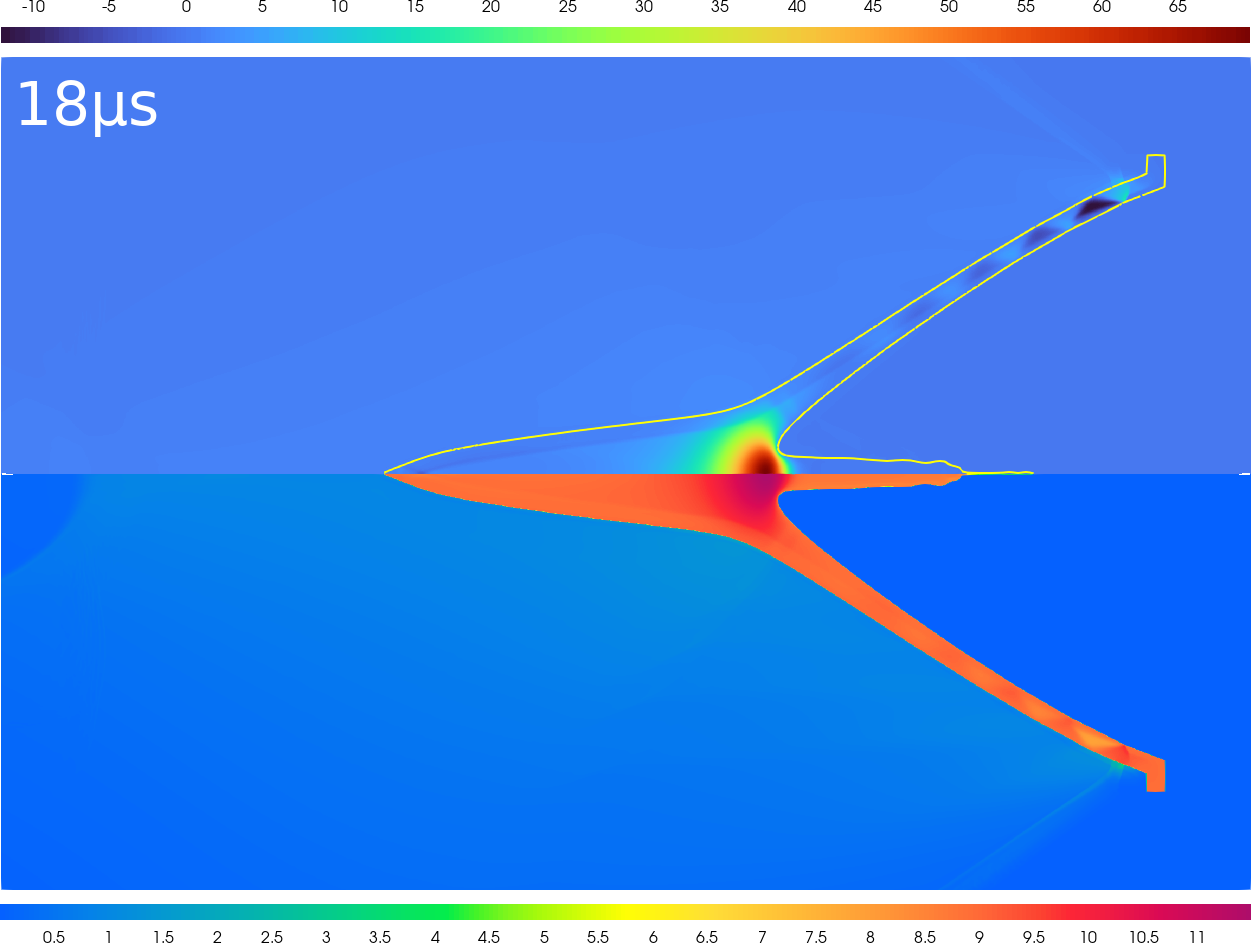
(d)

(e)

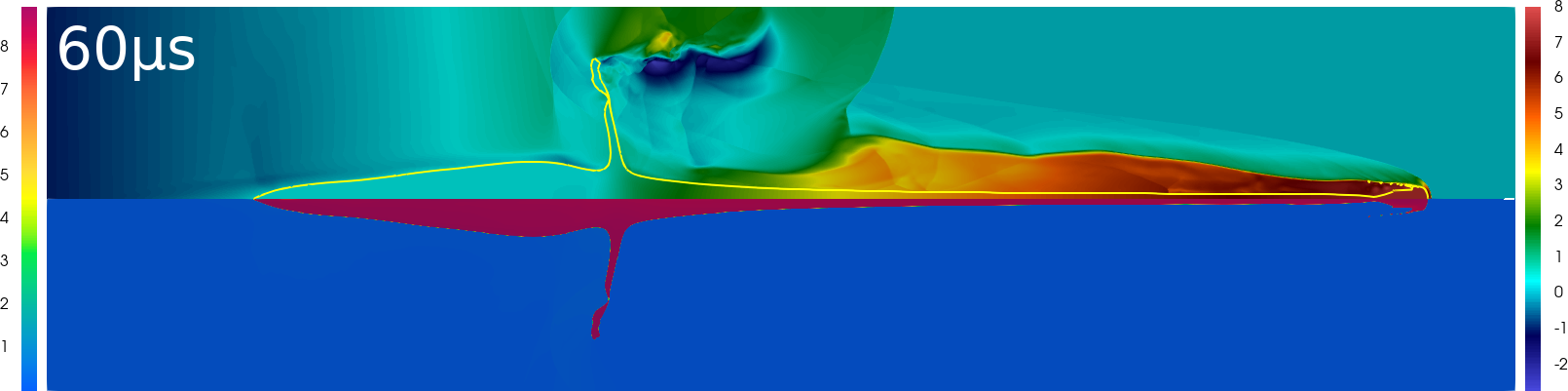
(f)

Figure 15: Time evolution of the shaped charge problem. (a)–(d) shows the HE burn and the liner collapse during the first eighteen microseconds. In each panel, the top half shows pressure measured in $\mathrm{GPa}$ and the bottom half shows density measured in $\mathrm{g\,cm}^{-3}$. (e) and (f) show the late-time jet formation at $t=45$ and $60\,\mu\mathrm{s}$. The top half of each panel shows the axial speed measured in $\mathrm{mm}\,\mu\mathrm{s}^{-1}$ and the bottom half shows the density. The yellow line denotes the $\phi=0.5$ contour.

Figure 16(a) shows the time history of the velocity of each Lagrangian tracer particle over the course of the simulation. The inner apex of the liner is accelerated close to the detonation velocity of the Comp-B ($7.98\,\mathrm{mm}\,\mu\mathrm{s}^{-1}$). By the end of the simulation the particle velocities have stabilised. Figure 16(b) shows the slice corresponding to $t=60\,\mu\mathrm{s}$ as a function of the initial $z$-coordinate of each tracer particle. The experimental results from [2] are overlaid. The jet velocity is particularly sensitive to the parameters used in the reactive burn model which have not been tuned, but nevertheless a fairly good match is obtained.

(a)

(b)

Figure 16: (a) shows the time history of the velocity of each Lagrangian tracer particle, initially distributed along the inner liner. (b) shows the stabilised jet velocity at $t=60\,\mu\mathrm{s}$ as a function of the initial position of each Lagrangian particle, alongside the tabulated experimental results from [2], where the error bars correspond to a $5\%$ uncertainty.

6 Conclusions

We have presented a novel Godunov-type volume-of-fluid method for the simulation of large deformation multi-material problems featuring elasto-plastic solids and fluids. The method can be viewed as an interface-sharpening extension to the diffuse-interface method of Barton [5]. The method is practical, robust and extensible, and has been shown capable of treating a range of challenging problems with excellent fidelity.

References

- [1] G. Allaire, S. Clerc, and S. Kokh. A five-equation model for the simulation of interfaces between compressible fluids. Journal of Computational Physics, 181(2):577–616, 2002.
- [2] F.E. Allison and R. Vitali. An application of the jet-formation theory to a 105mm shaped charge. Technical Report AD0277458, Army Ballistic Research Lab, Aberdeen Proving Ground, MD, 1962.
- [3] A.J. Barlow, R.N. Hill, and M.J. Shashkov. Constrained optimization framework for interface-aware sub-scale dynamics closure model for multimaterial cells in lagrangian and arbitrary lagrangian–eulerian hydrodynamics. Journal of Computational Physics, 276:92–135, 2014.
- [4] A.J. Barlow, P.H. Maire, W.J. Rider, R.N. Rieben, and M.J. Shashkov. Arbitrary lagrangian–eulerian methods for modeling high-speed compressible multimaterial flows. Journal of Computational Physics, 322:603–665, 2016.
- [5] P.T. Barton. An interface-capturing godunov method for the simulation of compressible solid-fluid problems. Journal of Computational Physics, 390:25–50, 2019.
- [6] P.T. Barton, R. Deiterding, D. Meiron, and D. Pullin. Eulerian adaptive finite-difference method for high-velocity impact and penetration problems. Journal of Computational Physics, 240:76–99, 2013.
- [7] P.T. Barton, D. Drikakis, and E.I. Romenskii. An eulerian finite-volume scheme for large elastoplastic deformations in solids. International Journal for Numerical Methods in Engineering, 81(4):453–484, 2010.
- [8] P.T. Barton, D. Drikakis, E.I. Romenskii, and V.A. Titarev. Exact and approximate solutions of riemann problems in non-linear elasticity. Journal of Computational Physics, 228(18):7046–7068, 2009.
- [9] P.T. Barton, B. Obadia, and D. Drikakis. A conservative level-set based method for compressible solid/fluid problems on fixed grids. Journal of Computational Physics, 230(21):7867–7890, 2011.
- [10] D.J. Benson. Computational methods in lagrangian and eulerian hydrocodes. Computer Methods in Applied Mechanics and Engineering, 99(2):235–394, 1992.
- [11] D.J. Benson. Volume of fluid interface reconstruction methods for multi-material problems. Applied Mechanics Reviews, 55(2):151–165, 04 2002.
- [12] M. Cutforth, P.T. Barton, and N. Nikiforakis. A volume-of-fluid reconstruction based interface sharpening algorithm for a reduced equation model of two-material compressible flow. Computers & Fluids, 231:105158, 2021.
- [13] V.N. Dorovskii, A.M. Iskol’Dskii, and E.I. Romenskii. Dynamics of impulsive metal heating by a current and electrical explosion of conductors. Journal of Applied Mechanics and Technical Physics, 24(4):454–467, 1983.
- [14] W. Zhang et al. AMReX: A Framework for Block-Structured Adaptive Mesh Refinement. Journal of Open Source Software, 4(37):1370, 2019.
- [15] N. Favrie and S.L. Gavrilyuk. Diffuse interface model for compressible fluid – compressible elastic–plastic solid interaction. Journal of Computational Physics, 231(7):2695–2723, 2012.
- [16] N. Favrie, S.L. Gavrilyuk, and R. Saurel. Solid–fluid diffuse interface model in cases of extreme deformations. Journal of Computational Physics, 228(16):6037–6077, 2009.
- [17] R.P. Fedkiw, T. Aslam, B. Merriman, and S. Osher. A non-oscillatory eulerian approach to interfaces in multimaterial flows (the ghost fluid method). Journal of Computational Physics, 152(2):457–492, 1999.
- [18] D.J. Hill, D. Pullin, M. Ortiz, and D. Meiron. An eulerian hybrid weno centered-difference solver for elastic–plastic solids. Journal of Computational Physics, 229(24):9053–9072, 2010.
- [19] C.W. Hirt and B.D. Nichols. Volume of fluid (vof) method for the dynamics of free boundaries. Journal of Computational Physics, 39(1):201–225, 1981.
- [20] B.P. Howell and G.J. Ball. A free-lagrange augmented godunov method for the simulation of elastic–plastic solids. Journal of Computational Physics, 175(1):128–167, 2002.
- [21] C.S. Jog. The explicit determination of the logarithm of a tensor and its derivatives. Journal of Elasticity, 93:141–148, 2008.
- [22] E. Johnsen and T. Colonius. Implementation of weno schemes in compressible multicomponent flow problems. Journal of Computational Physics, 219(2):715–732, 2006.
- [23] G.R. Johnson and W.H. Cook. Fracture characteristics of three metals subjected to various strains, strain rates, temperatures and pressures. Engineering Fracture Mechanics, 21(1):31–48, 1985.
- [24] M. Klima, A.J. Barlow, M. Kucharik, and M.J. Shashkov. An interface-aware sub-scale dynamics multi-material cell model for solids with void closure and opening at all speeds. Computers & Fluids, 208:104578, 2020.
- [25] S. Kokh and F. Lagoutière. An anti-diffusive numerical scheme for the simulation of interfaces between compressible fluids by means of a five-equation model. Journal of Computational Physics, 229(8):2773–2809, 2010.
- [26] M. Kucharik, R.V. Garimella, S.P. Schofield, and M.J. Shashkov. A comparative study of interface reconstruction methods for multi-material ale simulations. Journal of Computational Physics, 229(7):2432–2452, 2010.
- [27] J.W. Kury, H.C. Hornig, E.L. Lee, J.L. McDonnel, D.L. Ornellas, M. Finger, F.M. Strange, and M.L. Wilkins. Metal acceleration by chemical explosives. In Fourth Symposium on Detonation, pages 3–13, 1965.
- [28] M. Larcher and F. Casadei. Explosions in complex geometries—a comparison of several approaches. International journal of protective structures, 1(2):169–195, 2010.
- [29] E.L. Lee, H.C. Hornig, and J.W. Kury. Adiabatic expansion of high explosive detonation products. Technical Report UCRL-50422, University of California Radiation Laboratory, 1968.
- [30] E.L. Lee and C.M. Tarver. Phenomenological model of shock initiation in heterogeneous explosives. The Physics of Fluids, 23(12):2362–2372, 1980.
- [31] I.N. Lomov, R. Pember, J. Greenough, and B. Liu. Patch-based adaptive mesh refinement for multimaterial hydrodynamics. In Joint Russian-American Five-Laboratory Conference on Computational Mathematics/Physics, 6 2005.
- [32] A. López Ortega, M. Lombardini, D.I. Pullin, and D.I. Meiron. Numerical simulation of elastic–plastic solid mechanics using an eulerian stretch tensor approach and hlld riemann solver. Journal of Computational Physics, 257:414–441, 2014.
- [33] V. Maltsev, M. Skote, and P. Tsoutsanis. High-order methods for diffuse-interface models in compressible multi-medium flows: A review. Physics of Fluids, 34(2):021301, 2022.
- [34] R. Menikoff. Jwl equation of state. Technical Report LA-UR-15-29536, Los Alamos National Laboratory, 2015.
- [35] L. Michael and N. Nikiforakis. A multi-physics methodology for the simulation of reactive flow and elastoplastic structural response. Journal of Computational Physics, 367:1–27, 2018.
- [36] G.H. Miller and P. Colella. A high-order eulerian godunov method for elastic–plastic flow in solids. Journal of Computational Physics, 167(1):131–176, 2001.
- [37] G.H. Miller and P. Colella. A conservative three-dimensional eulerian method for coupled solid–fluid shock capturing. Journal of Computational Physics, 183(1):26–82, 2002.
- [38] G.H. Miller and E.G. Puckett. A high-order godunov method for multiple condensed phases. Journal of Computational Physics, 128(1):134–164, 1996.
- [39] M.J. Murphy, E.L. Lee, A.M. Weston, and A.E. Williams. Modeling shock initiation in composition b. In Tenth symposium on detonation, Boston, MA, 1993.
- [40] S. Osher and J.A. Sethian. Fronts propagating with curvature-dependent speed: Algorithms based on hamilton-jacobi formulations. Journal of Computational Physics, 79(1):12–49, 1988.
- [41] J.E. Pilliod and E.G. Puckett. Second-order accurate volume-of-fluid algorithms for tracking material interfaces. Journal of Computational Physics, 199(2):465–502, 2004.
- [42] B.J. Plohr and D.H. Sharp. A conservative eulerian formulation of the equations for elastic flow. Advances in Applied Mathematics, 9(4):481–499, 1988.
- [43] J.J. Quirk and S. Karni. On the dynamics of a shock–bubble interaction. Journal of Fluid Mechanics, 318:129–163, 1996.
- [44] R. Saurel and C. Pantano. Diffuse-interface capturing methods for compressible two-phase flows. Annual Review of Fluid Mechanics, 50(1):105–130, 2018.
- [45] S. Schoch, K. Nordin-Bates, and N. Nikiforakis. An eulerian algorithm for coupled simulations of elastoplastic-solids and condensed-phase explosives. Journal of Computational Physics, 252:163–194, 2013.
- [46] M.J. Shashkov. Closure models for multimaterial cells in arbitrary lagrangian–eulerian hydrocodes. International Journal for Numerical Methods in Fluids, 56(8):1497–1504, 2008.
- [47] M.J. Shashkov and E. Kikinzon. Moments-based interface reconstruction, remap and advection. Journal of Computational Physics, 479:111998, 2023.
- [48] R.K. Shukla, C. Pantano, and J.B. Freund. An interface capturing method for the simulation of multi-phase compressible flows. Journal of Computational Physics, 229(19):7411–7439, 2010.
- [49] K. Shyue and F. Xiao. An eulerian interface sharpening algorithm for compressible two-phase flow: The algebraic thinc approach. Journal of Computational Physics, 268:326–354, 2014.
- [50] K.K. So, X.Y. Hu, and N.A. Adams. Anti-diffusion interface sharpening technique for two-phase compressible flow simulations. Journal of Computational Physics, 231(11):4304–4323, 2012.
- [51] V.A. Titarev, E.I. Romenskii, and E.F. Toro. Musta-type upwind fluxes for non-linear elasticity. International Journal for Numerical Methods in Engineering, 73(7):897–926, 2008.
- [52] B. Van Leer. Towards the ultimate conservative difference scheme iii. upstream-centered finite-difference schemes for ideal compressible flow. Journal of Computational Physics, 23(3):263–275, 1977.
- [53] B. Van Leer. Towards the ultimate conservative difference scheme. iv. a new approach to numerical convection. Journal of Computational Physics, 23(3):276–299, 1977.
- [54] D. Verney. Evaluation de la limite élastique du cuivre et de l’uranium par des expériences d’implosion’lente’. In Behaviour of Dense Media Under High Dynamic Pressures, Symposium HDP, Paris, 1968.
- [55] T. Wallis, P.T. Barton, and N. Nikiforakis. A diffuse interface model of reactive-fluids and solid-dynamics. Computers & Structures, 254:106578, 2021.
- [56] T. Wallis, P.T. Barton, and N. Nikiforakis. A flux-enriched godunov method for multi-material problems with interface slide and void opening. Journal of Computational Physics, 442:110499, 2021.
- [57] W.N. Weseloh. Pagosa sample problem: Unconfined shaped charge. Technical Report LA-UR-16-20590, Los Alamos National Laboratory, 2016.
- [58] M.L. Wilkins and M.W. Guinan. Impact of cylinders on a rigid boundary. Journal of Applied Physics, 44(3):1200–1206, 1973.
- [59] S.D. Wilkinson, P.T. Barton, and N. Nikiforakis. A thermal equilibrium approach to modelling multiple solid–fluid interactions with phase transitions, with application to cavitation. International Journal of Multiphase Flow, 157:104234, 2022.
- [60] F. Xiao, Y. Honma, and T. Kono. A simple algebraic interface capturing scheme using hyperbolic tangent function. International Journal for Numerical Methods in Fluids, 48(9):1023–1040, 2005.
- [61] D.L. Youngs. Time-dependent multi-material flow with large fluid distortion. Numerical Methods for Fluid Dynamics, 1982.