Tensor network approach to the fully frustrated XY model on a kagome lattice with a fractional vortex-antivortex pairing transition

Abstract

We have developed a tensor network approach to the two-dimensional fully frustrated classical XY spin model on the kagome lattice, and clarified the nature of the possible phase transitions of various topological excitations. We find that the standard tensor network representation for the partition function does not work due to the strong frustrations in the low temperature limit. To avoid the direct truncation of the Boltzmann weight, based on the duality transformation, we introduce a new representation to build the tensor network with local tensors lying on the centers of the elementary triangles of the kagome lattice. Then the partition function is expressed as a product of one-dimensional transfer matrix operators, whose eigen-equation can be solved by the variational uniform matrix product state algorithm accurately. The singularity of the entanglement entropy for the one-dimensional quantum operator provides a stringent criterion for the possible phase transitions. Through a systematic numerical analysis of thermodynamic properties and correlation functions in the thermodynamic limit, we prove that the model exhibits a single Berezinskii-Kosterlitz-Thouless phase transition only, which is driven by the unbinding of $1/3$ fractional vortex-antivortex pairs determined at $T_{c}\simeq 0.075J_{1}$ accurately. The absence of long-range order of chirality or quasi-long range order of integer vortices has been verified in the whole finite temperature range. Thus the long-standing controversy about the phase transitions in this fully frustrated XY model on the kagome lattice is solved rigorously, which provides a plausible way to understand the charge-6e superconducting phase observed experimentally in the two-dimensional kagome superconductors.

I Introduction.

Various two dimensional (2D) kagome lattice models have attracted a lot of interest in the study of the interplay between band topology, geometric frustrations and strong correlations in the past decades. Due to the special lattice geometry with corner-sharing triangles, the kagome lattice features exotic electronic structures, such as flat bands, van Hove singularity and non-trivial topology of Dirac conesMielke (1991); Neupert et al. (2022); Yin et al. (2022); Jiang et al. (2023). The strongly geometric frustrations can induce massive degenerate ground states in kagome spin lattice models, providing one of the most promising platforms to realize quantum spin liquidsBalents (2010); Norman (2016); Zhou et al. (2017); Broholm et al. (2020). In addition to these intriguing phenomena, the unusual kagome superconductivity (SC) has recently been intensively investigated in the family of quasi-2D materials AV₃Sb₅ (A=K, Rb, Cs) (Ref. Ortiz et al. (2019, 2020, 2021); Jiang et al. (2021); Liang et al. (2021)). One of the exciting discoveries is the possible vestigial charge-6e SC around the superconducting transitionGe et al. (2022).

Different from the conventional SC described by the Bardeen-Cooper-Schrieffer theory as condensation of charge-2e Cooper pairs, the charge-4e or -6e SC can emerge as a vestigial higher-order condensation of bound states of electron sextets above the critical temperature of charge-2e SC (Ref.Kivelson et al. (1990); Röpke et al. (1998); Wu (2005); Agterberg and Tsunetsugu (2008); Berg et al. (2009); Ko et al. (2009); Herland et al. (2010); Jiang et al. (2017); Fernandes and Fu (2021); Jian et al. (2021); Song and Zhang (2022a); Agterberg et al. (2011); Struck et al. (2011); You et al. (2012)). It seems that the charge-6e SC has a close relation to certain types of pair density wave states on a hexagonal latticeChen et al. (2021). The most important feature of the charge-6e SC is characterized by the fractional magnetic flux quantization of $h/6e$. Despite the latest experimental progress, many basic properties of charge-6e SC remain less well understood. Some theoretical studiesAgterberg et al. (2011); Zhou and Wang (2022); Pan et al. (2022) have suggested that the charge-6e SC may be resulted from the fluctuations of pair density wave order. Nevertheless, the experimental realization of such charge-6e SC has not been verified so far.

Despite the lack of direct physical origin and implication of these remarkable observations, the crucial ingredient of the underlying geometry frustrations provides an insightful perspective to understand the charge-6e SC. The exotic quantum phenomena of charge-6e SC can naturally be caused by the effect of strong frustrations of the kagome geometry. At the phenomenology level, a complex SC order parameter can be expressed as $|\psi(\vec{r})|e^{i\theta(\vec{r})}$. When the amplitude fluctuations of $|\psi(\vec{r})|$ is frozen, the SC transition is governed by the phase fluctuations of the Cooper pairs, and the essential physics is described by a classical ferromagnetic XY spin modelBeasley et al. (1979); Emery and Kivelson (1995); Carlson et al. (1999); Li et al. (2007). However, in the presence of an external magnetic field, the ferromagnetic coupling between the nearest-neighbor (NN) XY spins may be tuned to be antiferromagnetic when each triangle of the kagome lattice has a $\pi$ fluxRzchowski (1997); Park and Huse (2001), which is the fully frustrated XY spin model. Such a model exhibits a large ground state degeneracy and fractional topological excitations because of the interference on the underlying lattice topologyHarris et al. (1992); Rzchowski (1997); Cherepanov et al. (2001); Park and Huse (2001); Korshunov (2002); Andreanov and Fistul (2020).

For the 2D antiferromagnetic XY kagome lattice model, apart from the global $U(1)$ spin rotational degrees of freedom, the frustration in each elementary triangle can induce the chiral degrees of freedom. To minimize the energy of each triangular plaquette, the orientation of the corresponding three XY spins should be different from each other by an angle of $2\pi/3$. In this way, when these three spins rotate clockwise or anti-clockwise, each plaquette can be ascribed a positive or negative chirality, displayed in Fig 1. In addition to the degeneracy associated with $U(1)$ symmetry, the ground state has a finite residual entropy of $0.126k_{B}$ per site, similar to the $3$-state antiferromagnetic Potts modelBaxter (1970); Huse and Rutenberg (1992). At low temperatures, the fluctuations of chirality are so strong that the phase angle between two spins separated by a long distance can freely change by $\pm 2\pi/3$. This uncertainty in the phase difference increases with distance and destroys the quasi-long-range order (quasi-LRO) in the XY spins. The absence of the quasi-LRO of the XY spins $\exp(i\theta)$ implies that the phase coherence of the charge-2e SC is absent.

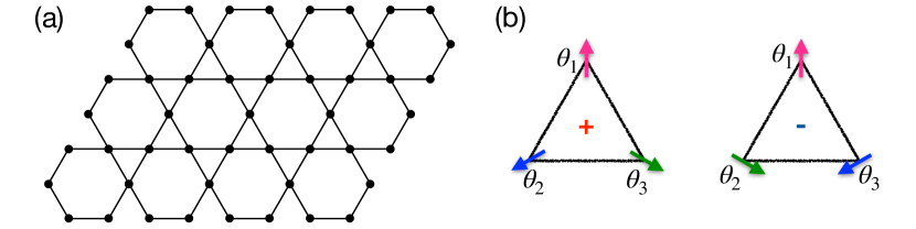
Figure 1: (a) The kagome lattice with anti-ferromagnetic nearest neighbor couplings. (b) Triangular plaquette with $+$ and $-$ chirlaity.

Although many theoretical conjectures were proposed, there has not yet had a general consensus on the existence of the phase with LRO arrangement of chirality at low temperatures. Some studiesHarris et al. (1992); Korshunov (2002) argued that the spin wave fluctuations favor the LRO of the anti-ferromagnetic arrangement of chirality for the neighboring triangular plaquettes and the phase coherence between integer vortices survives, while some other worksRzchowski (1997); Cherepanov et al. (2001); Park and Huse (2001); Andreanov and Fistul (2020) suggested that the chirality is always disordered corresponding to the suppression of the conventional charge-2e SC and the lowest-order quantity displaying quasi-LRO is given by the $\exp(i3\theta)$ variables. Due to the presence of strong frustrations and massive degeneracy of the ground state, it reminds a challenging problem to clarify the low temperature phases of the anti-ferromagnetic XY model on the kagome lattice. The reason for the numerical difficulty is that the excitations of different kinds of topological excitations (integer vortices, $1/3$ fractional vortices, domain walls, and kinks on the domain walls) occur close to each other at rather low transition temperatures of nearly $1/11$ of the usual non-frustrated Berezinskii-Kosterlitz-Thouless (BKT) transitionRzchowski (1997). And the traditional sampling methods often suffer from the finite size effects and a critical slowing down when approaching to the low temperature phaseSwendsen and Wang (1987); Wolff (1989); Andreanov and Fistul (2020).

Fortunately, the recent developments in tensor network (TN) methods have shed new light on the numerical study of 2D classical frustrated spin systemsVanderstraeten et al. (2018); Vanhecke et al. (2021); Song and Zhang (2022b); Colbois et al. (2022). It is found that the construction of the TN representations of the partition functions should be carried out with special care to encode the underlying physics of all the ground-state configurations at the level of local tensors. The convergence problem of the contraction algorithms of TN can be overcome by suitable Hamiltonian tessellations or split of $U(1)$ spins. In this work, we develop a peculiar TN approach to numerically solve the anti-ferromagnetic XY model on kagome lattices. Different from the discrete cases of $Z_{2}$ spinsVanhecke et al. (2021); Colbois et al. (2022) or the fully frustrated XY spin model on a square lattice with a chiral LRO ground stateSong and Zhang (2022b), the choice of the TN representations for the fully frustrated kagome lattice model does not affect the convergence of the contraction algorithms, but it does lead to incorrect contraction values at low temperatures. We find that the standard formulation is not always a good option, because the finite truncation of the Boltzmann weights fails to represent the massive degeneracy of the ground states. Here we have to introduce a special construction strategy based on the duality transformationsJosé et al. (1977); Knops (1977); Cherepanov et al. (2001), and then the partition function is transformed into an infinite 2D TN with local tensors lying on the centers of the elementary triangles of the original kagome lattice, which can be efficiently contracted by a recently proposed TN algorithm under optimal variational principlesZauner-Stauber et al. (2018); Fishman et al. (2018); Vanderstraeten et al. (2019a).

Once the proper implementation of TN representation is achieved, it can be expressed in terms of a product of 1D transfer matrix operator. The singularity of the entanglement entropy of this 1D quantum transfer operator can be used to determine various phase transitions with good accuracyHaegeman and Verstraete (2017). The distinct advantage of the TN method is that a stringent criterion can be used to distinguish various phase transitions without identifying any order parameter a prior. From the perspective of the quantum entanglement, we determine the phase structure of the anti-ferromagnetic XY model on the kagome lattices with clear evidence that only a single phase transition takes place at $T_{c}\simeq 0.075J_{1}$. From the analysis of the thermodynamic properties and the behavior of XY spin correlation functions, we demonstrate the phase transition belongs to the BKT universality classBerezinskii (1971); Kosterlitz and Thouless (1973); Kosterlitz (1974) driven by the unbinding of $1/3$ fractional vortex-antivortex pairs. In the absence of LRO in chirality, the low temperature phase is characterized by a quasi-LRO in the spin variable $\exp(i3\theta)$, while the phase coherence of integer vortices is destroyed due to the exponential decaying of the $\exp(i\theta)$ correlation functions. The clarification of such a phase gives rise to a prototype example, where the conventional charge-2e SC of the Cooper pairs is suppressed, but an unusual form of charge-6e SC of “Cooper sextuples” survives.

The rest of the paper is organized as follows. In Sec. II, we give an introduction of the 2D fully frustrated XY model on the kagome lattice and the possible phase transitions. In Sec. III, we develop a general framework of the TN method for this fully frustrated model based on the crucial duality transformation. In Sec. IV, we present the numerical results for the determination of the finite temperature phase diagram. Finally in Sec. V, we give our conclusions and future extensions of our work.

II Model Hamiltonian and topological excitations

We start with the effective Ginzburg-Landau (GL) free-energy density of superconductivity in an external gauge field

$$\mathcal{F}_{GL}=a|\psi|^{2}+\frac{b}{2}|\psi|^{4}+\frac{1}{2m^{\ast}}\left|\left(\frac{\hbar}{i}\nabla-\frac{e^{\ast}}{c}\vec{A}\right)\psi\right|^{2},$$ (1)

where $a$, $b$ are phenomenological expansion coefficients dependent on the materials, $m^{\ast}=2m_{e}$ and $e^{\ast}=2e$ are the effective mass and the charge of Cooper pairs, and the energy of the inductive fields $\vec{B}=\nabla\times\vec{A}$ produced by the supercurrents are ignoredPark and Huse (2001). The complex order parameter $\psi(\vec{r})=\langle c_{\uparrow}^{\dagger}(\vec{r})c_{\downarrow}^{\dagger}(\vec{r})\rangle$ can be regarded as a wave function for the Cooper pairs and expressed as $\psi(\vec{r})=|\psi(\vec{r})|\mathrm{e}^{i\theta(\vec{r})}$. Since the fluctuations of $|\psi(\vec{r})|$ can be ignored in the low temperature regime, we reduce the above GL free energy to a classical XY spin model on a 2D kagome lattice with the model HamiltonianTeitel and Jayaprakash (1983)

$$H=-J_{1}\sum_{\langle ij\rangle}\cos\left(\theta_{i}-\theta_{j}+A_{ij}\right),$$ (2)

where $J_{1}=\frac{n_{s}\hbar^{2}}{m^{\ast}}$ is the coupling strength with the superfluid density fixed as $n_{s}=|\psi(\vec{r})|^{2}$, $i$ and $j$ enumerate the lattice sites, $\theta_{i}$ can be regarded as classical XY spins associated with each lattice site and the summation is over all pairs of the nearest neighbors. The frustration is induced by the gauge field defined on the lattice bond satisfying $A_{ij}=-A_{ji}$. The gauge field is related to the vector potential by $A_{ij}=\frac{2\pi}{\Phi_{0}}\int_{\vec{r}_{i}}^{\vec{r}_{j}}d\vec{l}\cdot\vec{A}$, where $\Phi_{0}=\frac{h}{2e}$ is the flux quantum.

In the absence of external magnetic field, the effective coupling is ferromagnetic and results in a conventional BKT phase transition to the low temperature state with power-law correlations of the XY spins, corresponding to the charge-2e SC. The corresponding physics of this transition has been well-established, which does not depend on the specifics of the lattice structure. To introduce strong frustrations into this model, we should have a $Z_{2}$ gauge field (one-half quantum flux per plaquette) $\sum_{\langle i,j\rangle\in\triangle}A_{ij}\equiv\pi\pmod{2\pi}$, where the summation is taken around the perimeter of each elementary triangle. Note that the direct physical origin of the gauge field in realistic kagome SC materials is still unclear, which may be resulted from the external magnetic fieldsTeitel and Jayaprakash (1983); Rzchowski (1997); Park and Huse (2001).

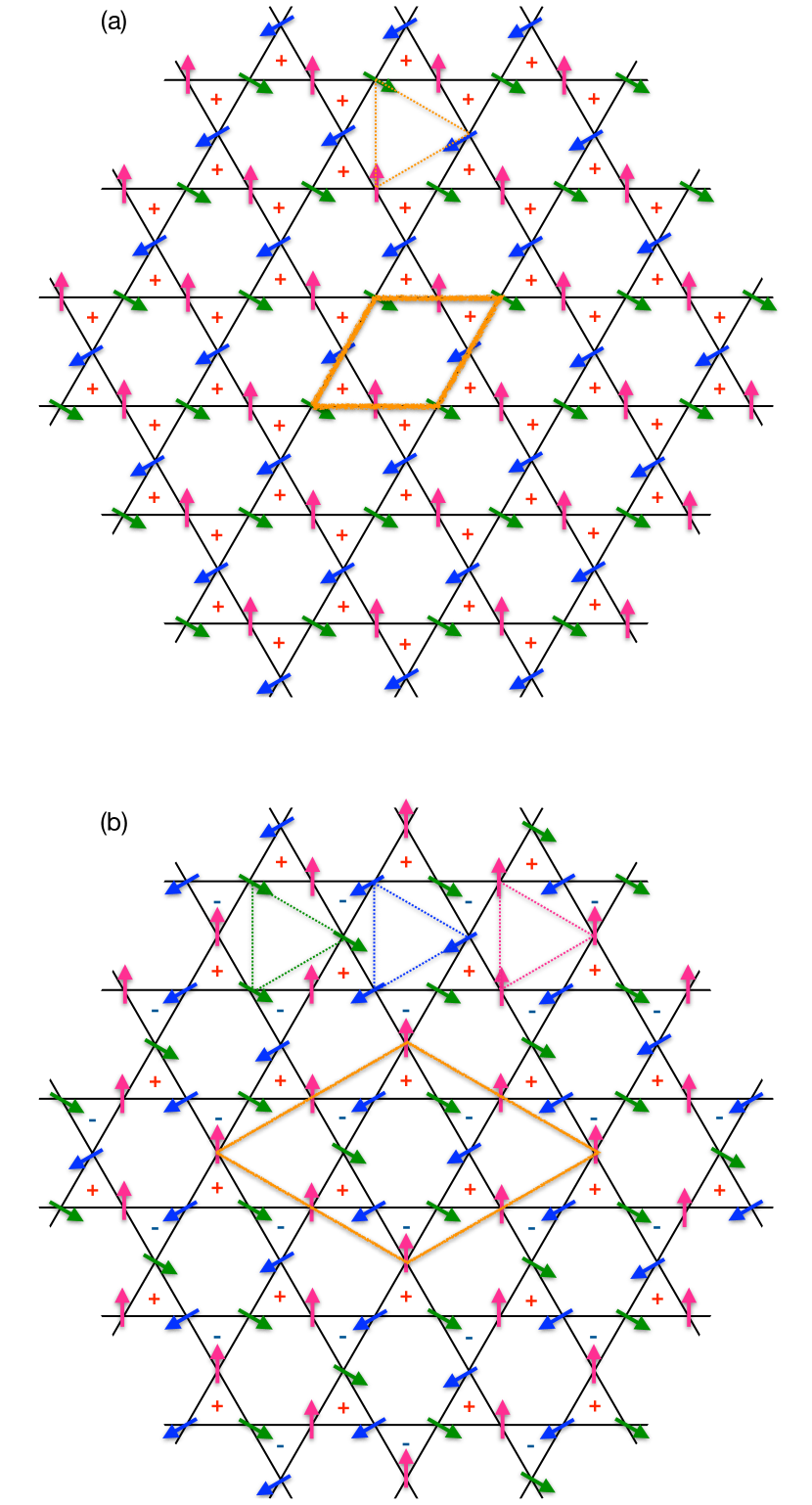
Figure 2: Two periodic patterns of chirality. Each pattern has another $Z_{2}$ degenerate state by switching the positive and negative chirality. The translational invariant units are represented by orange parallelograms, respectively. (a) One of the two $q=0$ patterns with a ferromagnetic arrangement of chiralities. (b) One of the two $\sqrt{3}\times\sqrt{3}$ patterns with a regular alternation of positive and negative chiralities.

Then the model Hamiltonian of the anti-ferromagnetic XY model on the kagome lattices is given by

$$H=J_{1}\sum_{\langle i,j\rangle}\cos(\theta_{i}-\theta_{j}),$$ (3)

where each elementary triangular plaquette is frustrated due to the anti-ferromagnetic interactions. To achieve the minimum of the energy, the angle between each pair of nearest neighbor spins should be $\pm 2\pi/3$. In addition to the global $U(1)$ rotation of all spins related to the global invariance of the Hamiltonian like the 2D classical XY model, the elementary triangular plaquette can be characterized by the chirality $\sigma=\pm 1$. The positive and negative chiralities of the plaquette are displayed in Fig 1 (b), corresponding to the anti-clockwise and clockwise rotation of the spins, respectively. The ground states of the anti-ferromagnetic XY model on a kagome lattice present a massive accidental degeneracy described by the $3$-state anti-ferromagnetic Potts model, which can also be mapped onto a solid-on-solid model at its roughening transitionHuse and Rutenberg (1992).

The accidental degeneracy of the ground state can be reduced to $U(1)\times Z_{2}$ in the presence of next-to-nearest neighbors (NNN) interactions:

$$H=J_{1}\sum_{\langle i,j\rangle}\cos(\theta_{i}-\theta_{j})+J_{2}\sum_{\langle\langle i,j\rangle\rangle}\cos(\theta_{i}-\theta_{j}),$$ (4)

where $J_{2}$ is the coupling between NNN sites denoted by $\langle\langle i,j\rangle\rangle$. For the anti-ferromagnetic NNN interaction ($J_{2}>0$), the spin pattern of the ground state has the same translational period as the usual kagome lattices, which is called the “$q=0$ state” shown in Fig 2 (a). For the ferromagnetic NNN interactions ($J_{2}<0$), the ground state of the spin pattern is called the “$\sqrt{3}\times\sqrt{3}$ state” with a regular alternation of positive and negative chiralities. Such a pattern has a translational invariant unit including three hexagons with a linear dimension $\sqrt{3}$ times larger than the unit cell of the original kagome lattice as displayed in Fig 2 (b).

Although extensive studies were carried out for this anti-ferromagnetic XY model on 2D kagome lattices in the past decades, the nature of the phase transitions in the frustrated model is still controversial Harris et al. (1992); Rzchowski (1997); Cherepanov et al. (2001); Park and Huse (2001); Korshunov (2002); Andreanov and Fistul (2020). The focus of the problem is whether the degeneracy of the chiralities could be lifted strongly enough to drive the system into a phase with LRO arrangement of chirality. Some studiesHarris et al. (1992); Korshunov (2002) proposed that the spin wave fluctuations would favor the LRO of the anti-ferromagnetic arrangement of chirality for the neighboring triangular plaquettes ($\sqrt{3}\times\sqrt{3}$ state) at low temperatures through a mechanism called “order by disorder”. Due to the $U(1)\times Z_{2}$ degeneracy, two kinds of topological excitations are expected to exist: (i) linear defects as the domain walls separating two ground states of different chirality patterns, (ii) point-like defects as vortices or anti-vortices which destroy the $U(1)$ phase coherence. Fig. 3 (a) displays the zero-energy domain walls separating the different $\sqrt{3}\times\sqrt{3}$ patterns. Each segment of the domain wall separates two triangular plaquettes with the same chirality and forms an angle of $2\pi/3$ between each other. Moreover, possible fractional vortices with topological charges of $\pm 1/3$ can exist on the kinks on the domain walls, where elementary links meet each other at a wrong angle not equal to $2\pi/3$. As displayed in Fig 3 (b), the kink separates the domain wall into two segments. Since the chiralities should be changed by the permutation of spin orientations within the elementary triangles when going across the segments, a discrepancy of $2\pi/3$ is introduced on a string connecting the kinks. The fractional vortices with the topological charge of $1/3$ thus form at the centers of the hexagons as the terminals of the string. Hence, the anti-ferromagnetic XY model on the kagome lattice should go through at least two kinds of phase transitions associated with the proliferation of the domain walls and the unbinding of fractional vortex pairs.

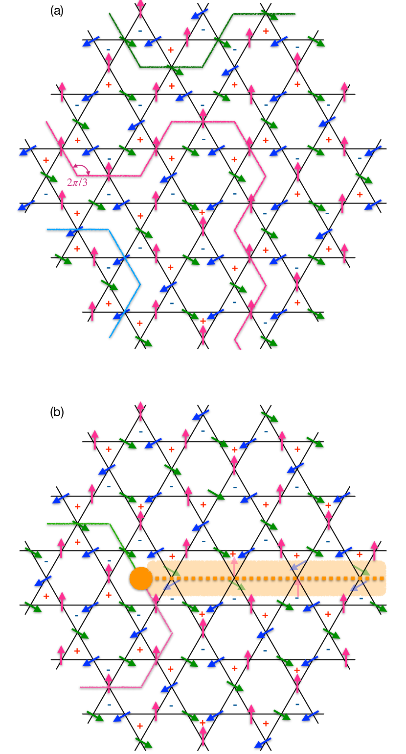
Figure 3: (a) Zero-energy domain walls (green, red and blue lines) separating two triangular plaquettes with the same chirality belonging to different $\sqrt{3}\times\sqrt{3}$ states. (b) Fractional vortices (orange circle) appear at every point where elementary links forming a domain wall meet each other at a wrong angle not equal to $2\pi/3$. The kink introduces a string (dotted line) with a discrepancy of $2\pi/3$ starting from the fractional vortex and terminating at another fractional vortex (not shown).

On the contrary, some other worksRzchowski (1997); Cherepanov et al. (2001); Park and Huse (2001); Andreanov and Fistul (2020) suggested that the chirality is always disordered with infinitely many ground states and $\exp(i3\theta)$ is the lowest-order quantity showing quasi-LRO. Instead of freezing into one specific pattern, the system would move among all possible patterns with the equilibrium probability given by the corresponding Boltzmann weights. Since the domain walls displayed in Fig 3 (a) can freely be excited, the physical pictures should be clearer by introducing the concept of excessive chargesKorshunov and Uimin (1986) rather than drawing complicated domain wall configurations. In this way, the topological charges of vortices on the centers of the hexagons can be defined by the chiralities of six surrounding triangles

$$q_{h}=\frac{1}{3}\sum_{t=1}^{6}q_{t},$$ (5)

where the charges $q_{t}=\pm\frac{1}{2}$ corresponds to chiralities $\sigma_{t}=\pm 1$, and the factor $\frac{1}{3}$ results from the fact that each triangle is shared by three neighboring hexagons. The relationships between the charges of vortices and the local domain wall configurations are enumerated in Fig 4. Another set of minus vortices configurations can be obtained by inverting all the signs of chiralities on the triangles. It is clear to see that the low temperature phase allows the free excitations of integer vortices of Fig 4 (a)-(c) and Fig 4 (h), while the fractional vortices shown in Fig 4 (d)-(g) are bound in pairs due to the higher energy cost. As shown in Fig 5, a pair of $\pm\frac{1}{3}$ vortices is created by switching the chiralities of two adjacent triangles. As the temperature increases, the fractional vortices will unbind at the BKT transition corresponding to the destruction of quasi-LRO in $e^{i3\theta}$.

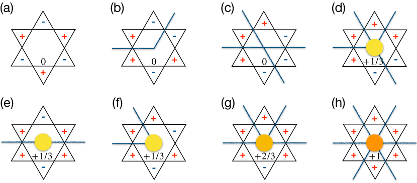
Figure 4: Topological charges of vortices corresponding to different domain wall structures. Another set of minus vortices can be obtained by inverting all the signs of chiralities. (a) Regular structure with zero charges. (b) Zero-energy domain wall with zero charges. (c) Intersection of two straight walls with zero charges. (d) Intersection of two walls with charge $+\frac{1}{3}$. (e) Domain wall of angle $\pi$ with charge $+\frac{1}{3}$. (f) Domain wall of angle $\frac{\pi}{6}$ with charge $+\frac{1}{3}$. (g) Intersection of two walls with charge $+\frac{2}{3}$. (h) Intersection of three straight walls with charge $+1$.

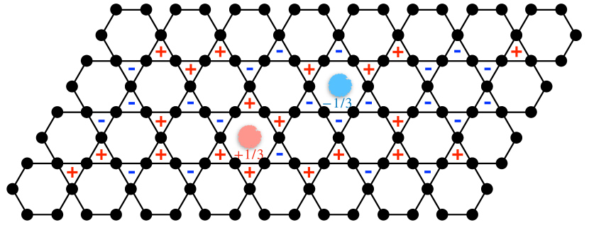
Figure 5: A pair of bound $\pm\frac{1}{3}$ vortices (red and blue circles) is created by switching the chiralities of two adjacent triangles of one of the degenerate minimum energy patterns.

III Tensor network theory

III.1 Problems in the standard representation

The partition function of a classical lattice model with local interactions can be always represented as a contraction of TN as a product of the transfer matrices on its original latticeZhao et al. (2010) or the dual latticeLevin and Nave (2007). The standard construction of the TN starts by putting a matrix on each bond accounting for the Boltzmann weight of the neighboring interactions. Then the local tensors can be obtained from suitable decompositions of the local bond matrices. Although this paradigm is proven a success in the studies of the classical ferromagnetic XY modelYu et al. (2014); Vanderstraeten et al. (2019b) and fully frustrated XY model on a square lattice with careful splits of $U(1)$ spins to encode the ground-state local rulesVanderstraeten et al. (2018); Vanhecke et al. (2021); Song and Zhang (2022b); Colbois et al. (2022), it cannot be directly applied to the frustrated XY kagome anti-ferromagnets, where a finite truncation of the interaction matrices fails to include the massive degeneracy of the low temperature phase.

To illustrate this problem, we first give the TN representation of the partition function from the generic approach. The partition function on the original lattice is expressed as

$$Z=\prod_{i}\int\frac{\mathrm{d}\theta_{i}}{2\pi}\prod_{\langle i,j\rangle}W(\theta_{i},\theta_{j}),$$ (6)

where $W(\theta_{i},\theta_{j})=\mathrm{e}^{-\beta J_{1}\cos(\theta_{i}-\theta_{j})}$ can be viewed as infinite interaction matrices with continuous $U(1)$ indices, and $\beta=1/k_{B}T$ is the inverse temperature with $k_{B}$ the Boltzmann constant. The partition function is then cast into the TN as shown in Fig. 6 (a), where the integrations $\int d\theta_{i}/2\pi$ are denoted as red dots and the matrix indices take the same values at the joint points.

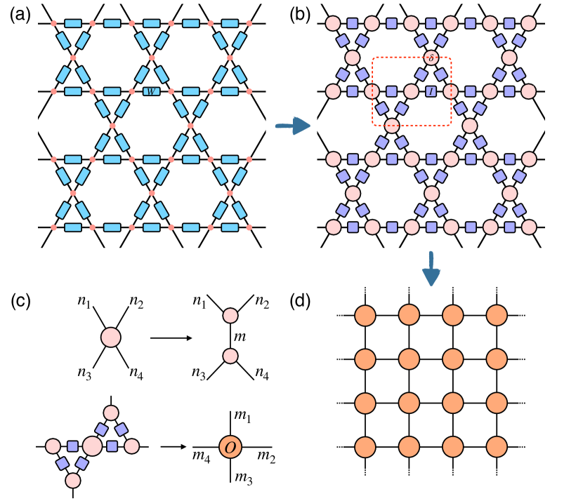
Figure 6: (a) The TN representation of the partition function with interaction matrices on the links accounting for the Boltzmann weight. (b) The TN representation of the partition function defined on the original lattice. The translation invariant cluster is circled by the red dotted line. (c) The split of the Kronecker delta functions and the construction of the local $O$ tensor. (d) The TN representation of the partition function composed of uniform local $O$ tensors.

To transform the local tensors onto a discrete basis, we employ the character decomposition

$$\mathrm{e}^{x\cos\theta}=\sum_{n=-\infty}^{\infty}I_{n}(x)\mathrm{e}^{in\theta}$$ (7)

to decompose the interaction matrices as

$$W(\theta_{i},\theta_{j})=\sum_{n_{l}}I_{n_{l}}(-\beta)\mathrm{e}^{in_{l}(\theta_{i}-\theta_{j})},$$ (8)

where $I_{n}(x)$ are the modified Bessel functions of the first kind. The index $n_{l}$ lies on the bond $l$ connecting NN sites with a direction from $i$ to $j$, which means $n_{l}=n_{(i,j)}=-n_{(j,i)}$. After integrating out the $U(1)$ phase degrees of freedom at each site, we get the partition function shown in Fig. 6 (b) in terms of the TN representation,

$$Z=\sum_{\{n_{l}\}}\prod_{l}I_{n_{l}}(-\beta)\prod_{i}\delta_{n_{1}(i)+n_{2}(i)+n_{3}(i)+n_{4}(i),0},$$ (9)

where the conservation law of $U(1)$ charges has been encoded in the local $\delta$ tensors. To obtain a uniform TN and avoid the splits of the spectrum tensors $I_{n}$ with the negative factor $(-1)^{n}$, we decompose the $\delta$ tensors, as two neighboring triangles share only one corner. As shown in Fig. 6 (c), we split a bigger 4-leg $\delta$ tensor into two smaller 3-leg $\delta$ tensors

$$n_{1}+n_{2}+n_{3}+n_{4}=0\quad\rightarrow\begin{cases}n_{1}+n_{2}+m=0\\ n_{3}+n_{4}+m=0\end{cases}.$$ (10)

Then we group the inner tensors composing the transitional invariant unit circled by the red dotted line in Fig. 6 (b) into a 4-leg $O$ tensor. Finally, the uniform TN displayed in Fig. 6 (d) is obtained as

$$Z=\mathrm{tTr}\prod_{s}O_{m_{1},m_{2}}^{m_{3},m_{4}}(s),$$ (11)

where “$\mathrm{tTr}$” means the tensor contraction over all auxiliary links and $s$ denotes the sites of the transitional invariant unit.

Unfortunately, such a construction does not work in the low temperature regime. Although the standard contraction algorithms converge for the construction of TN without a hitch, they lead to incorrect contraction results at low temperatures. The contraction values are found to be highly dependent on the truncation dimensions of the Boltzmann weight, i.e., the upper limit $n_{\max}$ of the Bessel function expansions $I_{n}(-\beta)$. The bond dimension $d$ of the $I$ tensor in Fig. 6 (b) is defined as $d=2n_{\max}+1$, where the index $n$ runs in the range $\{-n_{\max},\cdots,n_{\max}\}$. The free energy density shown in Fig. 7 is calculated directly from the partition function

$$f=-\frac{1}{\beta N}\ln Z,$$ (12)

where $N$ is the total number of sites on the original kagome lattice under contraction. We find that the free energy always displays an inflection point that shifts left with increasing bond dimensions $d$. The singular point in the free energy density seems to indicate the occurrence of a first-order phase transition, which turns out to be misleading seen in the following sections. The move of the inflection point stops around $T\simeq 0.08J_{1}$ and the data below this temperature displays strong fluctuations upon increasing $d$ thereafter.

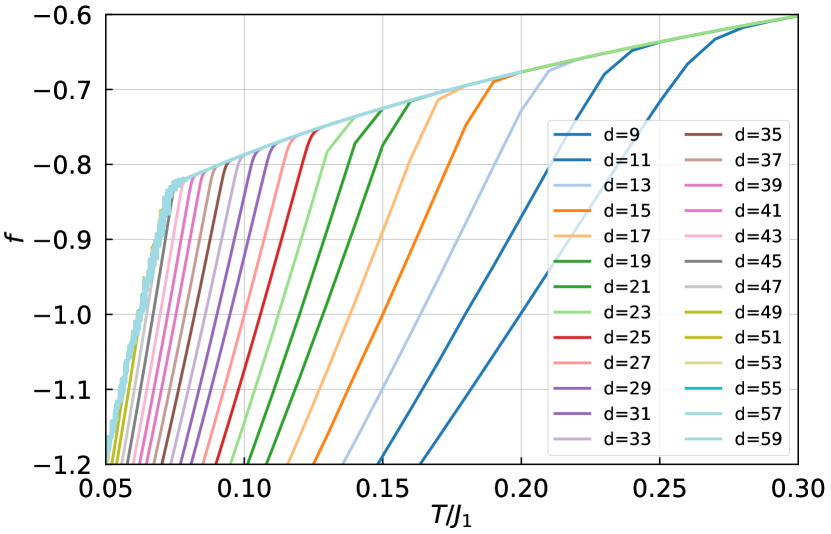
Figure 7: (a) The free energy obtained from the contraction of the TN constructed from direct truncations on the Boltzmann weight. The bond dimension $d$ denotes the upper limit of the Bessel function expansions.

The low temperature physics should be calculated with infinite bond dimension $d$ in principle, because the Bessel functions become $I_{n}(\beta)\gg 1$ with $\beta\gg 1$. However, for numerical calculations, a finite truncation on $d$ is necessary. The finite cutoff corresponds to the saturation of a maximal number of NN bonds, which is far away from the true ground state of infinite degeneracy due to the strong frustrations. That is why the standard construction is not applicable in the low temperature regime.

III.2 Duality transformation

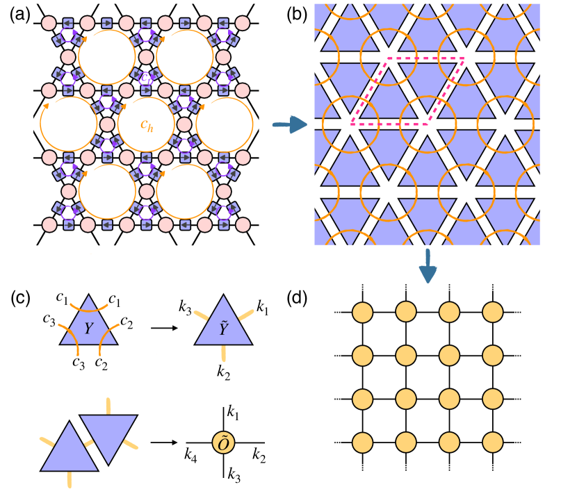
Figure 8: (a) The decompositions of $n_{l}$ at each kagome lattice bond in terms of integer-valued currents $c_{h}$ and $c_{t}$ circulating on the centers of elementary hexagons and triangles. (b) The TN consisting of local $Y$ tensors (purple triangles). The orange circles denote the hexagons currents $c_{h}$ and the dashed box denotes the transitional invariant unit. (c) The basis transformation from $Y$ tensor to $\tilde{Y}$ tensor and the construction of local $\tilde{O}$ tensor by combining two neighboring $\tilde{Y}$ tensors. (d) The TN representation of the partition function composed of uniform local $\tilde{O}$ tensors.

To avoid the direct truncation on Bessel function expansion $n$, we propose a new construction approach with the help of the duality transformationJosé et al. (1977); Knops (1977); Cherepanov et al. (2001). As shown in Fig. 8 (a), we decompose $n$ in terms of integer-valued currents circulating on the centers of elementary hexagons and triangles

$$n_{l}=c_{h}+c_{t},$$ (13)

where the arrows on the links denote the directions assigned to $n_{l}$. The negative value of $c_{h}$ or $c_{t}$ means the reverse direction of the current against $n_{l}$. In this way, the conservation condition on each site $n_{1}+n_{2}+n_{3}+n_{4}=0$ is satisfied automatically. And the partition function (9) is transformed into

$$Z=\sum_{\{c_{h},c_{t}\}}\prod_{l}I_{c_{h}+c_{t}}(-\beta).$$ (14)

Then the problem with finite truncations of the Bessel functions can be bypassed by performing an infinite sum over the triangle currents

$$Z=\sum_{\{c_{h}\}}\prod_{t}\sum_{c_{t}=-\infty}^{\infty}\prod_{h_{t}=1}^{3}I_{c_{h_{t}}+c_{t}}(-\beta),$$ (15)

where $h_{t}=1,2,3$ denote three hexagons surrounding each triangle $t$. Using the Fourier transformation

$$I_{n}(-\beta)=\frac{1}{2\pi}\int_{-\pi}^{\pi}d\theta\mathrm{e}^{-in\theta}\mathrm{e}^{-\beta\cos(\theta)},$$ (16)

we sum out the $c_{t}$ on each triangle and obtain

$$Y_{c_{1},c_{2},c_{3}} =\sum_{c_{t}=-\infty}^{\infty}\prod_{h=1}^{3}I_{c_{h}+c_{t}}(-\beta)$$ (17)

$$=\sum_{c_{t}=-\infty}^{\infty}\int\limits_{-\pi}^{\pi}\int\limits_{-\pi}^{\pi}\int\limits_{-\pi}^{\pi}\frac{d\phi_{1}d\phi_{2}d\phi_{3}}{(2\pi)^{3}}\mathrm{\exp}\left(-\sum_{h=1}^{3}[i(c_{h}+c_{t})\phi_{h}+\beta\cos\phi_{h}]\right)$$

$$=\int\limits_{-\pi}^{\pi}\int\limits_{-\pi}^{\pi}\frac{d\phi_{1}d\phi_{2}}{(2\pi)^{2}}\exp\left(-i[\phi_{1}(c_{1}-c_{3})+\phi_{2}(c_{2}-c_{3})]-\beta[\cos\phi_{1}+\cos\phi_{2}+\cos(\phi_{1}+\phi_{2})]\right).$$

Here $Y_{c_{1},c_{2},c_{3}}$ is referred to a 6-rank tensor with indices $c_{1}$, $c_{2}$ and $c_{3}$ displayed in Fig. 8 (b), where the neighboring indices at each corner of the triangle share the same $c_{h}$.

Since the transition temperature is quite lowRzchowski (1997), the integrand in (17) is saturated by the vicinity of the saddle points $\phi_{h}\sim\frac{2\pi\sigma_{t}}{3}$ in the low temperature limit ($\beta\gg 1$), where $\sigma_{t}=\pm 1$ is the chirality defined on the triangles related to infinite ground states. Substituting the asymptotic formula

$$Y_{c_{1},c_{2},c_{3}} \propto \sum_{\sigma_{t}=\pm 1}\int\limits_{-\pi}^{\pi}\int\limits_{-\pi}^{\pi}\frac{d\phi_{1}d\phi_{2}}{(2\pi)^{2}}\exp\left\{-i[\phi_{1}(c_{1}-c_{3})+\phi_{2}(c_{2}-c_{3})]-\frac{\beta}{2}[(\phi_{1}-\frac{2\pi\sigma_{t}}{3})^{2}+(\phi_{2}-\frac{2\pi\sigma_{t}}{3})^{2}]\right\}$$ (18)

$$= \sum_{\sigma_{t}=\pm 1}\exp\left\{-\frac{i2\pi\sigma_{t}}{3}(c_{1}+c_{2}+c_{3})-\frac{1}{3\beta}[(c_{1}-c_{3})^{2}+(c_{2}-c_{3})^{2}+(c_{3}-c_{1})^{2}]\right\},$$

back into the expression (15) and using the Poisson summation formula

$$\sum_{c=-\infty}^{\infty}\delta(\tilde{c}-c)=\sum_{m=-\infty}^{\infty}\mathrm{e}^{i2\pi m\tilde{c}},$$ (19)

we can write the partition function as

$$Z=\sum_{\{\sigma_{t}\},\{m_{h}\}}\left(\prod_{h}\int\limits_{-\infty}^{\infty}d\tilde{c}_{h}\right)\prod_{h}\exp\left[-i2\pi\sum_{t_{h}=1}^{6}(\frac{\sigma_{t_{h}}}{3}+m_{h})\tilde{c}_{h}-\frac{1}{3\beta}\sum_{\langle h,h^{\prime}\rangle}(\tilde{c}_{h}-\tilde{c}_{h^{\prime}})^{2}\right],$$ (20)

where $\tilde{c}$ are continuous currents and $m$ are integers defined on the centers of the hexagons. In the low temperature limit, the integration over $\tilde{c}$ gives the conservation conditions of chiralities surrounding each hexagon

$$\sum_{t_{h}=1}^{6}\sigma_{t_{h}}\equiv 0\pmod{6},$$ (21)

corresponding to the free excitations of integer vortices as shown in Fig 4 (a)-(c) and Fig 4 (h).

Since the values of $Y_{c_{1},c_{2},c_{3}}$ in (17) are just dependent on the difference of $c_{h}$ on the edges of the triangle, we can transform the $Y$ tensors onto a new basis

$$k_{1}=c_{1}-c_{2},\quad k_{2}=c_{2}-c_{3},\quad k_{3}=c_{3}-c_{1},$$ (22)

and obtain the 3-rank local tensors

$$\tilde{Y}_{k_{1},k_{2},k_{3}}=Y_{c_{1},c_{2},c_{3}}$$ (23)

as shown in Fig. 8 (c). Finally, the transitional invariant local tensor $\tilde{O}$ is achieved by combining a pair of up and down triangles. And the uniform TN representation of the partition function displayed in Fig. 8 (d) is given by

$$Z=\mathrm{tTr}\prod_{s}\tilde{O}_{k_{1},k_{2}}^{k_{3},k_{4}}(s).$$ (24)

From the asymptotic form (18), it is clear that the tensor components of $\tilde{Y}$ decrease exponentially with increasing $|k_{i}|$ ($i=1,2,3$). Hence we can truncate the series safely and approximate $\tilde{O}$ with a finite bond dimension $\tilde{d}$ in high precision, where $\tilde{d}=2k_{\max}+1$ with the index $k$ ranging from $-k_{\max}$ to $k_{\max}$.

III.3 Evaluations of the physical quantities

The fundamental object for the calculation of the partition function is the row-to-row transfer operator consisting of an infinite train of $\tilde{O}$ tensors

$$\hat{T}(\beta)=\sum_{\cdots,s,p,q,\cdots}\mathrm{Tr}\,\left[{\cdots\tilde{O}_{k_{1}}^{k_{3}}(s)\tilde{O}_{k_{1}}^{k_{3}}(p)\tilde{O}_{k_{1}}^{k_{3}}(q)\cdots}\right],$$ (25)

where $s,\ p,\ q,\ \cdots$ label different sites within a single row. This operator can be regarded as the matrix product operator (MPO) for 1D quantum spin chains of complicated interactions with the correspondence

$$\hat{H}_{\text{1D}}=-\frac{1}{\beta}\log\hat{T}(\beta).$$ (26)

In the thermodynamic limit, the partition function is determined by the dominant eigenvalue of the transfer operator as shown in Fig. 9 (a)

$$\hat{T}(\beta)|\Psi(A)\rangle=\Lambda_{\max}|\Psi(A)\rangle,$$ (27)

where $|\Psi(A)\rangle$ is the leading eigenvector represented by matrix product states (MPS) made up of uniform local $A$ tensorsZauner-Stauber et al. (2018). The local tensor $A_{\alpha,\beta}^{k}$ is a 3-leg tensor with physical bond dimension $\tilde{d}$ and auxiliary bond dimension $D$ controlling the accuracy of the approximation.

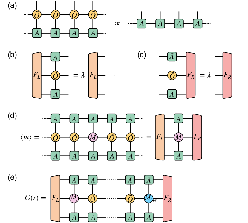
Figure 9: (a) Eigenequation for the fixed-point uniform MPS $|\Psi(A)\rangle$ of the 1D transfer operator $\hat{T}$. (b) and (c) Eigenequations for the left and right fixed-point eigenvectors of the channel operator $\mathbb{T}_{\tilde{O}}$. (d) Expectation of a local operator calculated by contracting the leading eigenvectors of the channel operators. (e) Two-point correlation function represented by contracting a train of channel operators.

The fixed-point eigen-equation can be accurately solved by the variational uniform matrix product state (VUMPS) algorithmZauner-Stauber et al. (2018); Fishman et al. (2018); Vanderstraeten et al. (2019a), which provides an efficient variational scheme to approximate the largest eigenvector $|\Psi(A)\rangle$. During the iteration of a set of optimized eigen-solvers, we also obtain the leading left and right eigenvectors of the channel operators. The channel operators have a sandwich structure composed of two local tensors of fixed point MPS and the middle four-leg local tensor. The channel operator related to $A$ tensor is defined by

$$\mathbb{T}_{X}=\sum_{i,j}\bar{A}^{i}\otimes X^{i,j}\otimes A^{j},$$ (28)

and other channel operators are defined in a similar way. The left and right fixed points of the channel operator $\mathbb{T}_{\tilde{O}}$ is obtained from the eigen-equations

$$\left\langle F_{L}\right|\mathbb{T}_{\tilde{O}}=\lambda\left\langle F_{L}\right|,\qquad\mathbb{T}_{\tilde{O}}\left|F_{R}\right\rangle=\lambda\left|F_{R}\right\rangle,$$ (29)

as displayed in Fig. 9 (b) and (c).

Once the fixed points are achieved, various physical quantities can be accurately calculated in the TN language. The entanglement properties can be detected via the Schmidt decomposition of $|\Psi(A)\rangle$ which bipartites the relevant 1D quantum state of the MPO,

$$|\Psi(A)\rangle=\sum_{\alpha,\beta=1}^{D}s_{\alpha}\delta_{\alpha,\beta}|\Psi_{\alpha}^{-\infty,n}\rangle|\Psi_{\beta}^{n+1,\infty}\rangle.$$ (30)

And the entanglement entropyVidal et al. (2003) is determined directly from the singular values $s_{\alpha}$ as

$$S_{E}=-\sum_{\alpha=1}^{D}s_{\alpha}^{2}\ln s_{\alpha}^{2},$$ (31)

in correspondence to the quantum entanglement measure.

Moreover, the expectation value of a local observable $m(\theta_{i})$ can be expressed as

$$m(\theta_{i})=\frac{1}{Z}\prod_{s}\int\frac{d\theta_{s}}{2\pi}\mathrm{e}^{-\beta E(\{\theta_{s}\})}m(\theta_{i}),$$ (32)

where $E(\{\theta_{s}\})$ is the energy of the state under a given spin configuration $\{\theta_{s}\}$. For the observables in the form of $m(\theta_{i})=\mathrm{e}^{iq\theta_{i}}$, it can be calculated by inserting the corresponding impurity tensors into the original tensor network for the partition function. The impurity tensor $M_{k_{1},k_{2}}^{k_{3},k_{4}}$ for the observable can be simply constructed by changing the corresponding charge conservation condition at site $i$ into

$$\sum_{l=1}^{4}n_{l}=q,$$ (33)

which introduces imbalanced currents in the local tensor $\tilde{Y}$ with the mapping $\tilde{Y}_{k_{1},k_{2},k_{3}}\rightarrow\tilde{Y}_{k_{1}+q,k_{2},k_{3}}$. Using the MPS fixed point, the contraction of the TN containing the impurity tensor is reduced to a trace of an infinite sequence of channel operators,

$$\langle m(\theta)\rangle=\mathrm{Tr}\,\left(\cdots\mathbb{T}_{\tilde{O}}\mathbb{T}_{\tilde{O}}\mathbb{T}_{M}\mathbb{T}_{\tilde{O}}\mathbb{T}_{\tilde{O}}\cdots\right),$$ (34)

which can be further squeezed into a contraction of a small network as shown in Fig. 9(d),

$$\langle m(\theta)\rangle=\langle F_{L}|\mathbb{T}_{M}|F_{R}\rangle$$ (35)

with the help of leading eigenvectors $\langle F_{L}|$ and $|F_{R}\rangle$.

In the same way, the two-point correlation function between local observables defined by $G(r)=\langle m(\theta_{j})m(\theta_{j+r})\rangle$ can be evaluated by inserting two local impurity tensors into the original TN. For the case of the spin-spin correlation function, the evaluation of $G(r)=\langle\mathrm{e}^{iq(\theta_{j}-\theta_{j+r})}\rangle$ is reduced to a trace of a row of channel operators containing two impurity tensors as shown in Fig. 9 (e)

$$G(r)=\langle F_{L}|\mathbb{T}_{M_{j}}\underbrace{\mathbb{T}_{O}\cdots\mathbb{T}_{O}}_{r-1}\mathbb{T}_{M_{j+r}}|F_{R}\rangle.$$ (36)

IV Numerical Results

In the previous sampling approaches the phase transitions were determined by some kinds of order parameter like the magnetization or Binder cumulent, where the corresponding numerical results of the simulations displayed a strong dependence on the system sizeRzchowski (1997); Andreanov and Fistul (2020) and a slow convergence under large frustrationsSwendsen and Wang (1987); Wolff (1989); Park and Huse (2001). Within the TN framework, we bring modern concepts of quantum entanglement to the frustrated classical XY model on the kagome lattices by mapping the transfer matrix to a 1D quantum transfer operator. The entanglement entropy of the fixed-point MPS for the 1D quantum correspondence exhibits singularity at the critical temperatures, which offers a sharp criterion to determine all possible phase transitions in the thermodynamic limit, especially for the systems possessing $U(1)$ and $Z_{2}$ degrees of freedomSong and Zhang (2021, 2022b, 2022a).

As shown in Fig. 10, the entanglement entropy $S_{E}$ develops only one sharp singularity at the critical temperature $T_{c}\simeq 0.075J_{1}$, which strongly indicates that a single phase transition takes place at a rather low temperature. As displayed in Fig. 10 (a), the entanglement entropies remain unchanged under different bond dimensions of the local $\tilde{O}$ tensor from $\tilde{d}=41$ to $47$. The convergence of the entanglement entropy demonstrates the success of the new construction approach. Moreover, the peak positions are almost unchanged with different MPS bond dimensions from $D=60$ to $120$ as shown in Fig. 10 (b). So we can accurately locate the transition temperature, which is in good agreement with theoretical expectationsCherepanov et al. (2001); Korshunov (2002) for the unbinding temperature of $1/3$ vortex pairs

$$T_{c}\approx\frac{\pi\sqrt{3}}{72}J_{1}\approx 0.075J_{1}.$$ (37)

Since the calculations are performed in the thermodynamic limit, we directly determine the transition temperature of the finite-size interpolation in the previous studies using sampling methodsRzchowski (1997). The specific advantage of the TN approach enables us to efficiently investigate the extremely low temperature regime that has never been reached before at a small cost of increasing MPO bond dimensions. As shown in Fig. 10 (c), the entanglement entropy is smooth everywhere at low temperatures, which demonstrates that there is no evidence for the selection of a single ground state of chirality down to $T\sim 10^{-5}J_{1}$. The temperature has reached low enough to rule out the possibility of ordering in staggered chirality, where the lower boundary of the transition temperature was just estimated to $T\sim 10^{-4}J_{1}$Korshunov (2002).

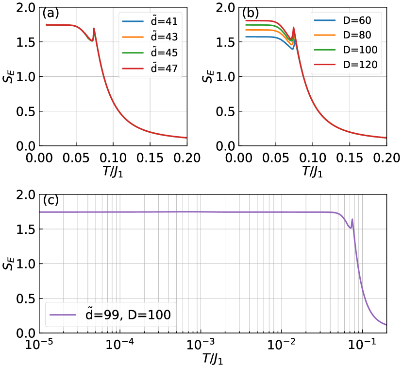
Figure 10: (a) The entanglement entropy as a function of temperature under MPS bond dimension $D=100$ and different MPO bond dimensions. (b) The entanglement entropy as a function of temperature under MPO bond dimension $\tilde{d}=45$ and different MPS bond dimensions. (c) The entanglement entropy at low temperatures under MPO bond dimension $\tilde{d}=99$ and MPS bond dimensions $D=100$.

For the sake of the possible periodic chirality pattern of $\sqrt{3}\times\sqrt{3}$ states, we also build the transfer operator with a larger unit cell consisting of $3\times 3$ clusters of $\tilde{O}$ tensors. The eigen-equation for the enlarged translational unit can be solved efficiently by the multiple lattice-site VUMPS algorithmNietner et al. (2020). We find that the lattice symmetry is not spontaneously broken and all the results are the same as the case of the simplest unit cell, which means the absence of the LRO of chirality.

Furthermore, we study the thermodynamic properties to understand the essential physics of the phase transition. The free energy per site can be calculated straightforwardly from the variational MPS setup

$$f=-\frac{1}{3\beta}\ln\lambda,$$ (38)

where $\lambda$ is the eigenvalue of the channel operators in (29) and the coefficient $\frac{1}{3}$ is due to the fact that each $\tilde{O}$ tensor contains three original kagome lattice sites. As displayed in Fig. 11 (a), it is clear that the free energy shows no signs of a first-order phase transition as it is perfectly smooth everywhere. The sharp contrast to the free energy in Fig. 7 obtained from the standard construction of TN demonstrates the success of our new construction approach.

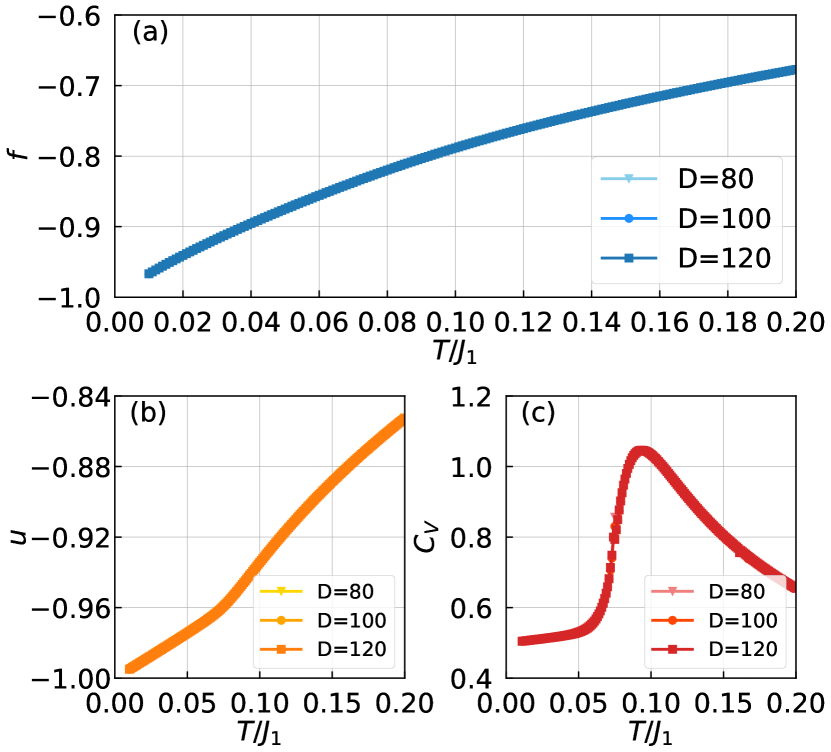
Figure 11: The thermodynamic properties under different MPS bond dimensions. (a) The free energy as a function of temperature. (b) The internal energy as a function of temperature. (c) The specific heat as a function of temperature.

The internal energy density can be obtained from the real part of the expectation value of the nearest-neighbor two-angle observable

$$u=2\langle\cos(\theta_{i}-\theta_{i+1})\rangle=2\mathrm{Re}\langle e^{i(\theta_{i}-\theta_{i+1})}\rangle\mathrm{.}$$ (39)

As shown in Fig. 11 (b), we find that there is no singularity in the temperature dependence of the internal energy. As the temperature approaches $T\rightarrow 0$, the internal energy converges to $u(T)\rightarrow-1$, which implies that the angle between the NN spins becomes $2\pi/3$ at the ground state. Also, the expectation value of chirality can be calculated as

$$\langle\sigma\rangle=\frac{2}{3\sqrt{3}}\sum_{\langle i,j\rangle\in\triangle}\sin(\theta_{i}-\theta_{j})$$ (40)

in the same way as the frustrated triangular latticesMiyashita and Shiba (1984). We find the expectation value of chirality equals zero with $\mathrm{Im}\langle e^{i(\theta_{i}-\theta_{i+1})}\rangle=0$ at all temperatures, which means the presence of strong fluctuations of chirality. Furthermore, the specific heat can be derived directly from

$$C_{V}=\frac{du}{dT},$$ (41)

which develops a round bump around $T=0.095J_{1}$ higher than the transition temperature determined from the entanglement entropy, which is a characteristic feature for the BKT transition. The smooth behavior of thermodynamic properties rules out the possibility of the first-order transition from the lifting of chirality degeneracyKorshunov (2002).

To further explore the nature of the phase transition, we calculate the following two different correlation functions among integer vortices and fractional vortices

$$G_{\theta}(r) =\langle\cos(\theta_{j}-\theta_{j+r})\rangle,$$

$$G_{3\theta}(r) =\langle\cos(3\theta_{j}-3\theta_{j+r})\rangle.$$ (42)

A comparison between these two correlation functions in the low temperature phase is shown in Fig. 12. For a given temperature of $T=0.07J_{1}<T_{c}$, the correlation function $G_{3\theta}(r)$ displays a power law behavior with distance but the correlation function $G_{\theta}(r)$ decays exponentially, corresponding to the presence of quasi-LRO of the fractional vortices and anti-vortices. As the temperature increases above $T_{c}$, both correlation functions behave in an exponential way, indicating that the system goes into the disordered phase. It is interesting to see that the correlation function $G_{\theta}(r)$ displays a dumped oscillation in the short range in accordance with the $\sqrt{3}\times\sqrt{3}$ pattern, but the fluctuation amplitude decays rapidly as shown in Fig. 12 (b). The exponential behavior in $\theta$ fields can be explained by the free fluctuations of the system among different ground-state chirality patterns. Although the spin wave fluctuations favor the short-range anti-ferromagnetic arrangement of chiralities, they are too weak to lift the ground-state degeneracy. The uncertainty of the phase difference of $\pm 2\pi/3$ increases with distance, which destroys the correlation in $\theta$ fields in the long range.

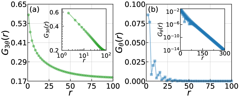
Figure 12: A comparison between different correlation functions at $T=0.07J_{1}$ below the BKT transition. (a) The correlation function of the $1/3$ fractional vortices exhibits a power law decay. (b) The correlation function of the integer vortices shows an exponential decay.

Such a behavior clearly indicates that the integer vortices can always excite freely, implying the absence of phase coherence between Cooper pairs at large distances. However, the $1/3$ fractional vortex pairs with quasi-LRO survive at low temperatures, which can be regarded as the condensation of Cooper sextuples. This phenomenon is just the characteristic of the charge-6e superconductivityGe et al. (2022). As the temperature increases, the system goes into the normal phase through a BKT transition driven by the dissociations of $1/3$ vortices.

V Conclusion and Outlook

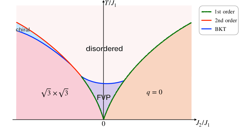
Figure 13: The schematic global phase diagram of the antiferromagnetic XY model with both NN and NNN interactions on kagome lattices defined by (4). The $q=0$ and $\sqrt{3}\times\sqrt{3}$ ordered states denote the LRO of the ferromagnetic and anti-ferromagnetic chirality pattern respectively, accompanying the quasi-LRO in the integer vortices. The FVP is the abbreviation for the fractional vortex-antivortex paired phase, where the $1/3$ fractional vortices are bounded in pairs in the absence of integer vortex-antivortex pairing. In the chiral phase, the phase coherence of either integer vortices or fractional vortices are destroyed while the anti-ferromagnetic chiral LRO survives.

Using the state-of-the-art TN methods, we have clarified the nature of the critical phase and phase transition of the fully frustrated classical XY model on 2D kagome lattice, which provides a plausible origin to the charge-6e SC discovered recentlyGe et al. (2022). We find standard construction approach of the TN for the partition function does not work due to the strong frustrations of the kagome lattice. To solve the issue of direct truncation of the Boltzmann weight, we have introduced a new method to build the TN based on duality transformation. Then the partition function is expressed as a product of 1D transfer matrix operators, whose eigen-equation is solved by the VUMPS algorithm accurately. The singularity of the entanglement entropy for this 1D quantum correspondence provides a stringent criterion for the temperature of possible phase transitions. Through a systematic analysis of thermodynamic properties and correlation functions in the thermodynamic limit, a single BKT transition is confirmed, which is driven by the unbinding of $1/3$ fractional vortex-antivortex pairs at $T_{c}\simeq 0.075J_{1}$. The absence of LRO of chirality or phase coherence between integer vortices is verified at all temperatures. Thus the long standing controversy about the phase transitions in the fully frustrated XY spin model on a kagome lattice is solved. The low temperature phase of the model can be interpreted as the presence of charge-6e SC but in the absence of the charge-2e SC.

An interesting open problem is to determine the full phase diagram with both the NN and NNN interactions described by (4). For both signs of the NNN interaction, the degeneracy of the ground state is lifted to $U(1)\times Z_{2}$. The possible global phase diagram is schematically described in Fig. 13. At low temperatures, the anti-ferromagnetic NNN interaction ($J_{2}>0$) will drive the system into the $q=0$ states with uniform chirality, while the ferromagnetic NNN interaction ($J_{2}<0$) drives the system into the $\sqrt{3}\times\sqrt{3}$ ordered state with a finite staggered chirality. The LRO of chirality allows the quasi-LRO of the integer vortices corresponding to the phase coherence of charge-2e SC. The phase transitions between the charge-2e SC and charge-6e SC states could be driven by proliferations of the low energy domain walls, which was supposed to be a first-order phase transition (the green lines) described by a six-state modelKorshunov (2002). And the phase boundary between the charge-6e SC state and the normal state still belongs to BKT transition (the blue line) driven by unbinding of $1/3$ fractional vortex-antivortex pairs. From the studies on the frustrated XY model on a triangular or square latticeLee and Lee (1998); Capriotti et al. (1998); Song and Zhang (2022b), we can expect that the staggered chiral LRO may survive above the BKT transition (the blue line) with an intermediate a chiral ordered phase. In this way, the boundary between the chiral ordered phase and disordered phase should be a second-order phase transition (the red line). We believe that our TN approach should provide a promising way to further investigate the fully frustrated XY on the kagome lattice with both NN and NNN interactions, giving rise to more interesting and fruitful insights into the exotic phenomena in the kagome superconducting materials.