Orientation selectivity of affine Gaussian derivative based receptive fields

Abstract

This paper presents a theoretical analysis of the orientation selectivity of simple and complex cells that can be well modelled by the generalized Gaussian derivative model for visual receptive fields, with the purely spatial component of the receptive fields determined by oriented affine Gaussian derivatives for different orders of spatial differentiation.

A detailed mathematical analysis is presented for the three different cases of either: (i) purely spatial receptive fields, (ii) space-time separable spatio-temporal receptive fields and (iii) velocity-adapted spatio-temporal receptive fields. Closed-form theoretical expressions for the orientation selectivity curves for idealized models of simple and complex cells are derived for all these main cases, and it is shown that the degree of orientation selectivity of the receptive fields increases with a scale parameter ratio $\kappa$, defined as the ratio between the scale parameters in the directions perpendicular to vs. parallel with the preferred orientation of the receptive field. It is also shown that the degree of orientation selectivity increases with the order of spatial differentiation in the underlying affine Gaussian derivative operators over the spatial domain.

We describe biological implications of the derived theoretical results, demonstrating that the predictions from the presented theory are consistent with previously established biological results concerning broad vs. sharp orientation tuning of visual neurons in the primary visual cortex. We also demonstrate that the above theoretical predictions, in combination with these biological results, are consistent with a previously formulated biological hypothesis, stating that the biological receptive field shapes should span the degrees of freedom in affine image transformations, to support affine covariance over the population of receptive fields in the primary visual cortex.

Based on the results from the theoretical analysis in the paper, combined with existing results for biological experiments, we formulate a set of testable predictions that could be used to, with neurophysiological experiments, judge if the receptive fields in the primary visual cortex of higher mammals could be regarded as spanning a variability over the eccentricity or the elongation of the receptive fields, and, if so, then also characterize if such a variability would, in a structured way, be related to the pinwheel structure in the visual cortex.

For comparison, we also present a corresponding theoretical orientation selectivity analysis for purely spatial receptive fields according to an affine Gabor model. The results from that analysis are consistent with the results obtained from the affine Gaussian derivative model, in the respect that the orientation selectivity becomes more narrow when making the receptive fields wider in the direction perpendicular to the preferred orientation of the receptive field. The affine Gabor model does, however, comprise one more degree of freedom in its parameter space, compared to the affine Gaussian derivative model, where a variability within that additional dimension of the parameter space does also strongly influence the orientation selectivity of the receptive fields. In this respect, the affine Gaussian derivative model leads to more specific predictions concerning relationships between the orientation selectivity and the elongation of the receptive fields, compared to the affine Gabor model.

1 Introduction

The receptive fields in the primary visual cortex (V1) capture properties of the visual patterns, which are then passed on to higher layers in the visual hierarchy. Being able to understand the computational function of these receptive fields is, hence, essential for understanding the computational function of the visual system.

The task of understanding the visual system has been addressed both neurophysiologically, by measuring the response properties of neurons to visual stimuli, and by formulating mathematical models, that aim at both explaining the computational function of visual neurons, as well as enabling computational simulation of neural functions in terms of biologically plausible computer vision algorithms, or aiming at making theoretical predictions, which can then be investigated experimentally.

Hubel and Wiesel (1959; 1962; 2005) pioneered the study of visual neurons in the primary visual cortex, and introduced the taxonomy of simple and complex cells. Simple cells were simple characterized by their properties of: (i) having distinct excitatory and inhibitory regions, (ii) obeying roughly linear summation properties, (iii) the excitatory and inhibitory regions balance each other in diffuse lighting. Visual neurons that did not obey these properties were referred to as complex cells, The response of a complex cell to a visual stimulus was also reported to be much less sensitive to the position of the stimulus in the visual field than for a simple cell.

More detailed characterizations of the receptive fields of simple cells have then been performed by DeAngelis et al. (1995; 2004), Ringach (2002; 2004), Conway and Livingstone (2006), Johnson et al. (2008) and De and Horwitz 2021), where specifically the use of multiple white noise stimuli permit a reconstruction of the full receptive field of a visual neuron, based on theoretical results in system identification theory, assuming linearity of the neuron. A more specialized methodology to characterize the response properties of possibly non-linear visual neurons, based on using deep predictive models to generate tailored stimuli for probing the neurons, has also been been more recently developed by Walker et al. (2019). Furthermore, more detailed characterizations of the orientation selectivity of visual neurons have been performed by Rose and Blakemore (1974), Schiller et al. (1976), Ringach et al. (2002), Nauhaus et al. (2008), Scholl et al. (2013) and Goris et al. (2015).

A detailed study of how the orientation selective of neurons in the primary visual cortex can be modulated for cats that wear permanently mounted googles, that alter the directional distribution of the incoming visual stimuli, has been presented by Sasaki et al. (2015), showing that long exposure to such stimuli affects the elongation of receptive fields, and how such elongation affects the orientational selectivity.

Mathematical models of simple cells have been formulated, in terms of Gabor filters (Marcelja 1980; Jones and Palmer 1987a; 1987b; Porat and Zeevi 1988) or Gaussian derivatives (Koenderink and van Doorn 1984; 1987; 1992; Young and his co-workers 1987; 2001; 2001, Lindeberg 2013; 2021). Specifically, theoretical models of early visual processes in terms of Gaussian derivatives have been formulated by Lowe (2000), May and Georgeson (2007), Hesse and Georgeson (2005), Georgeson et al. (2007), Wallis and Georgeson (2009), Hansen and Neumann (2008), Wang and Spratling (2016) and Pei et al. (2016).

Beyond the work by Hubel and Wiesel, the properties of complex cells have been further characterized by Movshon et al. (1978), Emerson et al. (1987), Touryan et al. (2002; 2005), Rust et al. (2005) and Goris et al. (2015), as well as modelled computationally by Adelson and Bergen (1985), Heeger (1992), Serre and Riesenhuber (2004), Einhäuser et al. (2002), Kording et al. (2004), Merolla and Boahen (2004), Berkes and Wiscott (2005), Carandini (2006) and Hansard and Horaud (2011).

The subject of this paper is to perform a detailed analysis of the orientation selectivity properties of models of simple and complex cells, based on image measurements in terms of affine Gaussian derivatives. The notion of affine Gaussian smoothing, with its associated notion of affine Gaussian derivatives, was derived axiomatically in (Lindeberg 2011) and was proposed as a spatial model of simple cells in (Lindeberg 2013; 2021). This model has also been extended to complex cells in (Lindeberg 2020 Section 5). Parallel extensions of the affine Gaussian derivative model for simple cells to spatio-temporal receptive fields have been performed in (Lindeberg 2016; 2021).

In this paper, we will build upon these latter works and perform an in-depth analysis of the orientation selectivity curves that result from the associated models of receptive fields for simple and complex cells. Specifically, we will focus on quantifying how the degree of orientation selectivity of a receptive field depends on how anisotropic or elongated that the underlying affine Gaussian derivatives are. We will derive explicit expressions for how the degree of orientation selectivity increases with the ratio between the scale parameters in the orientations perpendicular to vs. parallel with the preferred orientation of the receptive fields. In this way, we also demonstrate how closed form theoretical analysis is possible for the generalized Gaussian derivative model for visual receptive fields, which arises from the normative theory of visual receptive fields in (Lindeberg 2021).

We will then use these theoretical results to express possible indirect support for a biological hypothesis raised in (Lindeberg 2023b), concerning how the variability of the shapes of receptive fields may be related to the variability of image structures under natural image transformations. If we assume that the visual system should implement affine covariant receptive fields, to make it possible for the visual system to better estimate shape properties of surfaces in the world, such as local surface orientation, then the property of affine covariance would make it possible to compute better estimates of local surface orientation, compared to a visual system that does not implement affine covariance, or a sufficiently good approximation thereof.

Specifically, if the population of receptive fields would support affine covariance in the primary visual cortex, or sufficiently good approximations thereof, then such an ability would support the possibility of computing affine invariant image representations at higher levels in the visual hierarchy, or more realistically sufficiently good approximations thereof, over restricted subspaces or subdomains of the most general forms of full variability under spatial affine transformations of the visual stimuli.

We cannot expect that visual perception should be able to implement full affine invariance. For example, from the well-known experience, that it is much harder to read a text upside-down, it is clear that visual perception cannot be regarded as invariant to spatial rotations in the image domain. From the expansion of the orientations of visual receptive fields according to the pinwheel structure of higher mammals, we can, however, regard the population of receptive fields as supporting local rotational covariance. If we look at a slanted surface in the world, we can get a robust perception of its surface texture under substantial variations of the slant angle, thus showing a robustness of visual perception under stretchings of visual image patterns that correspond to non-uniform scaling transformations (the perspective effects on a slanted surface patch can to first-order of approximation be modelled as a stretching of the image pattern along the tilt direction in image space, complemented with a uniform scaling transformation). If the visual receptive fields would span a variability under such spatial stretching transformations, then such a variability would precisely correspond to a variability in the anisotropy, or the degree of elongation, of the receptive fields.

An overall theme of this article is to, based on a theoretical analysis of a relationship between the orientation selectivity and the degree of anisotropy or degree of elongation of receptive fields in the primary visual cortex, in combination with existing neurophysiological results concerning variabilities in the orientation selectivity of the receptive fields in relation to the pinwheel structure of higher mammals, address the question of whether the receptive fields in the primary visual cortex could be regarding as spanning a variability over the elongation of the receptive fields, to, in turn, support covariant image measurements under such variabilities, or, at least, sufficiently good approximations thereof.

If we, in particular, that if we could assume that the spatial components of the receptive fields could be well modelled by affine Gaussian derivatives, then the property of affine covariance implies that there should be visual receptive fields for different degrees of anisotropy present in the visual system. If we further combine the theoretical results to be derived in this paper, which will state that the degree of orientation selectivity is strongly dependent on the anisotropy or the elongation of the receptive fields, with the biological results established by Nauhaus et al. (2008), which show that the degree of orientation selectivity for neurons in the primary visual cortex varies both strongly and in relationship with the position on the cortical surface in relation to the pinwheel structure, then these results together are fully consistent with the hypothesis that the visual receptive fields in the primary visual cortex should span a variability in their anisotropy, thus consistent with the hypothesis that the receptive fields in the pinwheel structure should span at least one more degree of freedom in the affine group, beyond mere rotations (as already established in previous neurophysiological measurements regarding the pinwheel structure of the oriented receptive fields in the primary visual cortex of higher mammals).

We will also, more generally, use predictions from the presented theoretical analysis to formulate a set of explicit testable hypotheses, that could be either verified or rejected in future neurophysiological experiments, as well as formulate a set of quantitive measurements to be made, to characterize a possible variability in the anisotropy or elongation of receptive fields in the primary visual cortex, with special emphasis on the relationships between a possibly predicted variability in receptive field elongation and the pinwheel structure in the primary visual cortex of higher mammals.

To investigate how the predictions from the presented theory would be affected, if we would replace the theoretical model for the visual receptive fields with another class of models, we will also present a corresponding detailed orientation selectivity analysis for a purely spatial affine Gabor model of simple and complex cells. The results from this model will turn out to be consistent with the results obtained from the affine Gaussian derivative model, in the respect that the orientation selectivity becomes more narrow if we make the receptive fields wider in the direction perpendicular to the preferred orientation of the receptive field. The parameter space of the affine Gabor model does, however, comprise one more degree of freedom compared to the parameter space of the affine Gaussian derivative model, where a variability along that additional dimension does also strongly influence the orientation selectivity of the receptive fields. In this respect, the predictions concerning a relationship between the orientation selectivity and the elongation or eccentricity of the receptive fields are more specific for the affine Gaussian derivative model than for the affine Gabor model.

1.1 Structure of this article

This paper is organized as follows: Section 2 provides a theoretical background to this work, by describing the generalized Gaussian derivative model for visual receptive fields, both in the cases of a purely spatial domain, where the receptive fields are pure affine Gaussian derivatives, and for a joint spatio-temporal domain, where the affine Gaussian derivatives are complemented by temporal derivatives of either a non-causal Gaussian kernel over the temporal domain, or a genuine time-causal kernel, referred to as the time-causal limit kernel, as well as complemented with possible velocity adaptation, to enable Galilean covariance.

Beyond these models of simple cells, we do both review a previously formulated purely spatial model for complex cells, based on a Euclidean combination of scale-normalized affine Gaussian derivatives of orders 1 and 2, as well as propose two new spatio-temporal models for complex cells, based on image measurements in terms of affine Gaussian derivatives over the spatial domain, complemented by explicit temporal processing operations. Two special cases are treated in terms of either space-time separable spatio-temporal receptive fields, or velocity-adapted spatio-temporal receptive fields, with the latter tuned to particular motion directions and motion velocities in joint space-time.

Section 3 then performs a detailed mathematical analysis of the orientation selectivity of these models, over three main cases of either (i) a purely spatial domain, (ii) a space-time separable spatio-temporal domain, or (iii) a velocity-adapted spatio-temporal domain. In each of these main cases, we analyze the properties of simple cells of orders 1 and 2, corresponding to first- or second-order Gaussian derivatives, as well as the orientation selectivity properties for our models of complex cells.

Concerning simple cells, it is shown that both the pure spatial receptive fields and the joint spatio-temporal receptive fields have similar orientation selectivity properties, which only depend on the order of spatial differentiation and the degree of anisotropy of the receptive field. For complex cells, a different dependency is, however, derived for the model based on space-time separable receptive fields, as opposed to the models for either a purely spatial domain or a joint spatio-temporal domain based on velocity-adapted spatio-temporal receptive fields.

Section 4 then develops implications of the presented theoretical results for biological vision. Comparisons are made to previous work by Nauhaus et al. (2008), concerning relations between the degree of orientation selectivity of biological receptive fields and the positions of the corresponding neurons on the cortical surface in the primary visual cortex, in relation to the pinwheel structure.

Specifically, it is demonstrated that the predictions generated from the presented theory are consistent with the experimentally observed biological facts concerning broad orientation tuning of the receptive fields near the pinwheels and sharper orientation tuning further away. These variations in the degree of orientation selectivity are, in turn, consistent with the variations in the degree of orientation selectivity in our idealized models of receptive fields, under variations in the parameter $\kappa$, or its inverse entity, the eccentricity $\epsilon=1/\kappa$.

By combining our theoretical predictions with the experimental measurements of biological orientation selectivity, these similarities are specifically consistent with the previously formulated hypothesis that the shapes of visual receptive fields in the primary visual cortex should comprise a variability over the parameter $\kappa$ (or $\epsilon$) in the primary visual cortex, to support affine covariance of the family of receptive fields, to, in turn, enable more accurate determinations of cues to the 3-D structure of the world, such as estimates of local surface orientation.

To firmly determine whether these theoretically based predictions would actually hold in biological vision, we will formulate a set of explicit testable hypotheses, which could be either verified or rejected by neurophysiological experiments, as well as a set of quantitative measurement that, in the case that the theoretical predictions would hold, could be performed to characterize how a possible variability in the anisotropy of elongation of the receptive field could be related to the pinwheel structure of higher mammals.

To widen the scope of the treatment in the paper, beyond a theoretical analysis of properties of idealized visual receptive field models according to the generalized Gaussian derivative model for visual receptive fields, we will also in Section 5 perform a corresponding orientation selectivity analysis for an affine Gabor model of receptive fields, as well as give a derivation of affine covariant properties of a further generalized affine Gabor model, with the details of that analysis in Appendix A.2 and Appendix A.3.

Finally, Section 6 gives a summary and discussion about some of the main results, including suggestions concerning possible extensions of the presented work.

2 Receptive field models based on affine Gaussian derivatives

For modelling the response properties of simple cells, we will in this paper make use of the affine Gaussian derivative model for linear receptive fields, which has been theoretically derived in a principled axiomatic manner in (Lindeberg 2011), and then been demonstrated in (Lindeberg 2013; 2021) to well model the spatial properties of simple cells in the primary cortex, as established by neurophysiological measurements by DeAngelis et al. (1995; 2004) and Johnson et al. (2008); see Figures 16–17 in (Lindeberg 2021) for comparisons between biological receptive fields and computational models in terms of affine Gaussian derivatives, as will be used as a basis for the analysis in this paper.

In this section, we shall review main components of this theory, which we shall then build upon in the theoretical analysis in Section 3 concerning the orientation selectivity properties of these receptive field models, based on the affine Gaussian derivative model for simple cells over a purely spatial domain, as well as a corresponding generalized affine Gaussian derivative model for simple cells over a joint spatio-temporal domain. Based on these models of simple cells, we shall also define models for complex cells, both over a purely spatial image domain and over a joint spatio-temporal domain, where the joint spatio-temporal models are new. Since the analysis to be performed in Section 3 will make use of very specific properties of this receptive field model, while this model may be less known than the Gabor model for visual receptive fields, this review will be rather detailed, so as to be sufficiently self-contained, to support the theoretical analysis that will be later presented in Section 3.

2.1 Purely spatial model of simple cells

If we initially disregard the temporal dependencies of the simple cells, we can formulate a purely spatial model of linear receptive fields with orientation preference according to (Lindeberg 2021 Equation (23)), see (Lindeberg 2021 Figure 7) for illustrations of such receptive fields;

$$T_{simple}(x_{1},x_{2};\;\sigma_{\varphi},\varphi,\Sigma_{\varphi},m)\\ =T_{\varphi^{m},norm}(x_{1},x_{2};\;\sigma_{\varphi},\Sigma_{\varphi})=\sigma_{\varphi}^{m}\,\partial_{\varphi}^{m}\left(g(x_{1},x_{2};\;\Sigma_{\varphi})\right),$$ (1)

where

• $\varphi$ represents the preferred orientation of the receptive field,

• $\sigma_{\varphi}$ represents the amount of spatial smoothing in the direction $\varphi$ (in units of the spatial standard deviation),

• $\partial_{\varphi}^{m}=(\cos\varphi\,\partial_{x_{1}}+\sin\varphi\,\partial_{x_{2}})^{m}$ is an $m$:th-order directional derivative operator in the direction $\varphi$,

• $\Sigma_{\varphi}$ is a symmetric positive definite covariance matrix, with one of its eigenvectors aligned with the direction of $\varphi$, and

• $g(x;\;\Sigma_{\varphi})$ is a 2-D affine Gaussian kernel with its shape determined by the covariance matrix $\Sigma_{\varphi}$

  $$g(x;\;\Sigma_{\varphi})=\frac{1}{2\pi\sqrt{\det\Sigma_{\varphi}}}e^{-x^{T}\Sigma_{\varphi}^{-1}x/2}$$ (2)

  for $x=(x_{1},x_{2})^{T}$, and with one of the eigenvectors of $\Sigma_{\varphi}$ parallel to the orientation $\varphi$.

For $m=1$ and $m=2$, differentiation of the affine Gaussian kernel and introducing the following parameterization of the spatial covariance matrix

$$\Sigma_{\varphi}=\left(\begin{array}[]{cc}C_{11}&C_{12}\\ C_{12}&C_{22}\end{array}\right)$$ (3)

with

$$\begin{split}C_{11}&=\sigma_{1}^{2}\,\cos^{2}\varphi+\sigma_{2}^{2}\,\sin^{2}\varphi,\end{split}$$ (4)

$$\begin{split}C_{12}&=2\,(\sigma_{1}^{2}-\sigma_{2}^{2})\cos\varphi\sin\varphi,\end{split}$$ (5)

$$\begin{split}C_{22}&=\sigma_{1}^{2}\,\sin^{2}\varphi+\sigma_{2}^{2}\,\cos^{2}\varphi,\end{split}$$ (6)

as well as reformulating the arguments with respect to this more explicit parameterization, leads to the following explicit expressions, for an arbitrary preferred orientation $\varphi$:

$$\begin{split}T_{simple}(x_{1},x_{2};\;\sigma_{1},\sigma_{2},\varphi,1)=\end{split}$$

$$\begin{split}=\sigma_{1}\,(\cos(\varphi)\,\partial_{x_{1}}+\sin(\varphi)\,\partial_{x_{2}})\,g(x_{1},x_{2};\;\Sigma_{\varphi})\end{split}$$

$$\begin{split}=-\frac{(x_{1}\cos(\varphi)+x_{2}\sin(\varphi))}{2\pi\,\sigma_{1}^{2}\,\sigma_{2}}\times\end{split}$$

$$\begin{split}e^{-\frac{\left(\sigma_{1}^{2}+\sigma_{2}^{2}\right)\left(x_{1}^{2}+x_{2}^{2}\right)-(\sigma_{1}-\sigma_{2})(\sigma_{1}+\sigma_{2})(2x_{1}x_{2}\sin(2\varphi)+\cos(2\varphi)(x_{1}-x_{2})(x_{1}+x_{2}))}{4\sigma_{1}^{2}\sigma_{2}^{2}}}\end{split}$$ (7)

$$\begin{split}T_{simple}(x_{1},x_{2};\;\sigma_{1},\sigma_{2},\varphi,2)=\end{split}$$

$$\begin{split}=\sigma_{1}^{2}\,(\cos^{2}(\varphi)\,\partial_{x_{1}x_{1}}+2\cos(\varphi)\sin(\varphi)\,\partial_{x_{1}x_{2}}+\sin^{2}(\varphi)\,\partial_{x_{2}x_{2}})\,\end{split}$$

$$\begin{split}\quad\quad g(x_{1},x_{2};\;\Sigma_{\varphi})\end{split}$$

$$\begin{split}=\frac{\left(x_{1}^{2}+x_{2}^{2}-2\sigma_{1}^{2}+\cos(2\varphi)\left(x_{1}^{2}-x_{2}^{2}\right)+2x_{1}x_{2}\sin(2\varphi)\right)}{4\pi\,\sigma_{1}^{3}\,\sigma_{2}}\times\end{split}$$

$$\begin{split}e^{-\frac{\left(\sigma_{1}^{2}+\sigma_{2}^{2}\right)\left(x_{1}^{2}+x_{2}^{2}\right)-(\sigma_{1}-\sigma_{2})(\sigma_{1}+\sigma_{2})(2x_{1}x_{2}\sin(2\varphi)+\cos(2\varphi)(x_{1}-x_{2})(x_{1}+x_{2}))}{4\sigma_{1}^{2}\sigma_{2}^{2}}}.\end{split}$$ (8)

In the above expressions for the spatial receptive field model $T_{simple}$, the multiplication of the $m$:th-order directional derivative operator in the direction $\varphi$ by the spatial scale parameter $\sigma_{\varphi}$ in the same direction, implements scale-normalized derivatives (Lindeberg 1998) according to

$$\partial_{x_{1}^{\alpha_{1}}x_{2}^{\alpha_{2}},norm}=\sigma^{\gamma(\alpha_{1}+\alpha_{2})}\,\partial_{x_{1}^{\alpha_{1}}x_{2}^{\alpha_{2}}},$$ (9)

where we here, for simplicity, choose the scale normalization power $\gamma=1$ to simplify the following calculations.

This notion of spatial scale-normalized derivatives implies that we measure the amplitude of local spatial variations with respect to a given scale level, and makes it possible to define scale-invariant feature responses, that assume the same magnitude for input image structures of different spatial extent, provided that the spatial scale levels are adapted to the characteristic length of spatial variations in the image data. Specifically, this spatial scale normalization of the spatial receptive field response implies scale selective properties in the sense that the receptive field will produce its maximum response over spatial scales at a spatial scale proportional to a characteristic length in the image data.

Note that this model for the spatial dependency of simple cells, in terms of affine Gaussian derivatives, goes beyond the previous biological modelling results by Young (1987), in turn with very close relations to theoretical modelling results by Koenderink and van Doorn (1987; 1992), in that the spatial smoothing part of the receptive field is here spatially anisotropic, and thereby allows for higher orientation selectivity compared to defining (regular) Gaussian derivatives from partial derivatives or directional derivatives of rotationally symmetric Gaussian kernels, as used by Young and Koenderink and van Doorn. Direct comparisons with biological receptive fields, see Figures 16–17 in (Lindeberg 2021), also show that biological simple cells are more anisotropic than can be well modelled by directional derivatives of rotationally symmetric Gaussian kernels.

2.2 Purely spatial model of complex cells

In (Lindeberg 2020 Section 5) it was proposed that some of the qualitative properties of complex cells, of being both (i) polarity-independent, (ii) approximately phase-independent and (ii) not obeying a superposition principle, as opposed to polarity-dependent as well as strongly phase-dependent, as simple cells are, can modelled by combining first- and second-order directional affine Gaussian derivative responses of the form

$${\cal Q}_{\varphi,spat,norm}L=\sqrt{\frac{L_{\varphi,norm}^{2}+C_{\varphi}\,L_{\varphi\varphi,norm}^{2}}{\sigma_{\varphi}^{2\Gamma}}},$$ (10)

where

• $L_{\varphi,norm}$ and $L_{\varphi\varphi,norm}$ represent the results of applying scale-normalized directional affine Gaussian derivative operators of orders 1 and 2, respectively, according to (1), to the input image $f$:

  $$L_{\varphi,norm}(x_{1},x_{2};\;\sigma_{\varphi},\Sigma_{\varphi})=\\ =T_{\varphi,norm}(x_{1},x_{2};\;\sigma_{\varphi},\Sigma_{\varphi})*f(x_{1},x_{2}),$$ (11)

  $$L_{\varphi\varphi,norm}(x_{1},x_{2};\;\sigma_{\varphi},\Sigma_{\varphi})=\\ =T_{\varphi\varphi,norm}(x_{1},x_{2};\;\sigma_{\varphi},\Sigma_{\varphi})*f(x_{1},x_{2}),$$ (12)

• $C_{\varphi}>0$ is a weighting factor between first and second-order information, and

• $\Gamma\geq 0$ is a complementary scale normalization parameter, that we, however, henceforth will set to zero, to simplify the following treatment.

This model can be seen as an affine Gaussian derivative analogue of the energy model of complex cells proposed by Adelson and Bergen (1985) and Heeger (1992), specifically the fact that receptive fields similar to first- vs. second-order derivatives are reported to occur in pairs (De Valois et al. 2000), resembling properties of approximate quadrature pairs, as related by a Hilbert transform (Bracewell 1999, pp. 267–272). The model is also closely related to the proposal by Koenderink and van Doorn (1990) to sum up the squares of first- and second-order derivative response, in a corresponding way as cosine wave and sine wave responses are combined in a Euclidean manner, to get a more phase-independent response.

For a perfect quadrature pair of filters, the sum of the squares of the filter responses will be spatially constant for any sine wave of any frequency and phase. The quasi quadrature entity will instead have the property that the response will be spatially constant, or alternatively have only relatively moderate ripples, at or near the spatial scale level at which the quasi quadrature measure assumes its maximum value over spatial scales, provided that the value of the weighting parameter $C_{\varphi}$ is properly chosen. In this way, the quasi quadrature measure combines the responses of the first- and second-order affine Gaussian derivative operators in a complementary manner, where the first-order derivatives correspond to odd filters (antisymmetric under reflection) and the second-order derivatives to even filters (symmetric under reflection).

2.3 Joint spatio-temporal models of simple cells

’ For modelling the joint spatio-temporal behaviour of linear receptive fields with orientation preference, in (Lindeberg 2021 Section 3.2) the following model is derived from theoretical arguments, see (Lindeberg 2021 Figures 10-11 for illustrations)

$$\begin{split}T_{simple}(x_{1},x_{2},t;\;\sigma_{\varphi},\sigma_{t},\varphi,v,\Sigma_{\varphi},m,n)\end{split}$$

$$\begin{split}&=T_{{\varphi}^{m},{\bar{t}}^{n},norm}(x_{1},x_{2},t;\;\sigma_{\varphi},\sigma_{t},v,\Sigma_{\varphi})\end{split}$$

$$\begin{split}&=\sigma_{\varphi}^{m}\,\sigma_{t}^{n}\,\partial_{\varphi}^{m}\,\partial_{\bar{t}}^{n}\left(g(x_{1}-v_{1}t,x_{2}-v_{2}t;\;\Sigma_{\varphi})\,h(t;\;\sigma_{t})\right),\end{split}$$ (13)

where (for symbols not previously defined in connection with Equation (1))

• $\sigma_{t}$ represents the amount of temporal smoothing (in units of the temporal standard deviation),

• $v=(v_{1},v_{2})^{T}$ represents a local motion vector, in the direction $\varphi$ of the spatial orientation of the receptive field,

• $\partial_{\bar{t}}^{n}=(\partial_{t}+v_{1}\,\partial_{x_{1}}+v_{2}\,\partial_{x_{2}})^{n}$ represents an $n$:th-order velocity-adapted temporal derivative operator,

• $h(t;\;\sigma_{t})$ represents a temporal smoothing kernel with temporal standard deviation $\sigma_{t}$.

In the case of non-causal time (where the future can be accessed), the temporal kernel can be determined to be a 1-D Gaussian kernel

$$h(t;\;\sigma_{t})=\frac{1}{\sqrt{2\pi}\sigma_{t}}e^{-t^{2}/2\sigma_{t}^{2}},$$ (14)

whereas in the case of time-causal time (where the future cannot be accessed), the temporal kernel can instead be chosen as the time-causal limit kernel (Lindeberg 2016 Section 5)

$$h(t;\;\sigma_{t})=\psi(t;\;\sigma_{t},c),$$ (15)

defined by having a Fourier transform of the form

$$\hat{\Psi}(\omega;\;\sigma_{t},c)=\prod_{k=1}^{\infty}\frac{1}{1+i\,c^{-k}\sqrt{c^{2}-1}\,\sigma_{t}\,\omega},$$ (16)

and corresponding to an infinite set of first-order integrators coupled in cascade with specifically chosen time constants to enable temporal scale covariance, where the distribution parameter $c>1$ describes the ratio between adjacent discrete temporal scale levels in this temporal scale-space model.

In analogy with the spatial scale normalization in the previous purely spatial model, multiplication of the $n$:th-order velocity-adapted temporal derivative operator $\partial_{\bar{t}}^{n}$ by the temporal standard deviation $\sigma_{t}$ raised to the power of $n$ implements scale-normalized velocity-adapted temporal derivatives according to

$$\partial_{\bar{t},norm}^{n}=\sigma_{t}^{\gamma n}\,\partial_{\bar{t}}^{n},$$ (17)

as an extension of Equation (9) from the spatial to the temporal domain, see (Lindeberg 2017). Also here, for simplicity, we restrict ourselves to the specific choice of the scale normalization parameter $\gamma=1$. By this temporal scale normalization, the temporal component of the spatio-temporal receptive field will have scale selective properties, implying that it will produce its maximum response over temporal scales at a temporal scale proportional to a characteristic temporal duration of the temporal structures in the video data.

In Figure 18 in (Lindeberg 2021) it is demonstrated that this model well captures the qualitative properties of simple cells in the primary visual cortex, as established by neurophysiological cell recordings by DeAngelis et al. (1995; 2004), regarding both space-time separable receptive fields and velocity-adapted receptive fields, tuned to particular motion directions in joint space-time.

Note that these spatio-temporal models of simple cells go beyond the previous biological modelling results by Young and his co-workers (2001; 2001) in that: (i) the purely spatial smoothing component of the receptive field model is based on anisotropic Gaussian kernels as opposed to rotationally symmetric Gaussian kernels, (ii) this model also incorporates a truly time-causal model, that takes into explicit account that the future cannot be accessed in a real-world situation, and (iii) the parameterization of the spatio-temporal filter shapes is different, and more closely aligned to the inherent geometry of the imaging situation.

2.4 Joint spatio-temporal models of complex cells

2.4.1 Model based on space-time separable receptive fields

For modelling qualitative properties of complex cells over the joint spatio-temporal domain, we can extend the spatial quasi quadrature measure in (10) to the following spatio-temporal quasi quadrature measure that operates on a combination of spatial directional derivatives and temporal derivatives according to

$$({\cal Q}_{\varphi,sep,norm}L)^{2}=\left(\left(L_{\varphi,t,norm}^{2}+C_{t}\,L_{\varphi,tt,norm}^{2}\right)\right.\\ \left.+\,C_{\varphi}\left(L_{\varphi\varphi,t,norm}^{2}+C_{t}\,L_{\varphi\varphi,tt,norm}^{2}\right)\right)/(\sigma_{\varphi}^{2\Gamma_{\varphi}}\sigma_{t}^{2\Gamma_{t}}),$$ (18)

where the individual components in this expression are defined from space-time separable receptive fields according to

$$L_{\varphi,t,norm}(x_{1},x_{2},t;\;\sigma_{\varphi},\sigma_{t},0,\Sigma_{\varphi})=\\ =T_{\varphi,t,norm}(x_{1},x_{2},t;\;\sigma_{\varphi},\sigma_{t},0,\Sigma_{\varphi})*f(x_{1},x_{2},t),$$ (19)

$$L_{\varphi,tt,norm}(x_{1},x_{2},t;\;\sigma_{\varphi},\sigma_{t},0,\Sigma_{\varphi})=\\ =T_{\varphi,tt,norm}(x_{1},x_{2},t;\;\sigma_{\varphi},\sigma_{t},0,\Sigma_{\varphi})*f(x_{1},x_{2},t),$$ (20)

$$L_{\varphi\varphi,t,norm}(x_{1},x_{2},t;\;\sigma_{\varphi},\sigma_{t},0,\Sigma_{\varphi})=\\ =T_{\varphi\varphi,t,norm}(x_{1},x_{2},t;\;\sigma_{\varphi},\sigma_{t},0,\Sigma_{\varphi})*f(x_{1},x_{2},t),$$ (21)

$$L_{\varphi\varphi,tt,norm}(x_{1},x_{2},t;\;\sigma_{\varphi},\sigma_{t},0,\Sigma_{\varphi})=\\ =T_{\varphi\varphi,tt,norm}(x_{1},x_{2},t;\;\sigma_{\varphi},\sigma_{t},0,\Sigma_{\varphi})*f(x_{1},x_{2},t),$$ (22)

with the underlying space-time separable spatio-temporal receptive fields $T_{\varphi^{m},t^{n},norm}(x_{1},x_{2},t;\;\sigma_{\varphi},\sigma_{t},0,\Sigma_{\varphi})$ according to (2.3) for $v=0$.

In the expression (18), the quasi quadrature measure operates on both pairs of first- and second-order directional derivates as well as pairs of first- and second-order velocity-adapted derivatives simultaneously, aimed at balancing the responses of odd vs. even filter responses over both space or time in parallel.

This (new) spatio-temporal quasi quadrature measure constitutes an extension of the spatio-temporal quasi quadrature measure in (Lindeberg 2018 Section 4.2), by being additionally adapted to be selective to particular image orientations over the spatial domain, as opposed to being rotationally isotropic, as well as being based on affine Gaussian derivative operators, as opposed to partial derivatives of rotationally symmetric Gaussian kernels over the spatial domain.

This oriented spatio-temporal quasi quadrature measure will specifically inherit the qualitative properties of the previously presented purely spatial oriented quasi quadrature measure (39) in that it will be polarity-independent as well as much less sensitive to the phase in the input video data compared to the above models of simple cells.

2.4.2 Model based on velocity-adapted receptive fields

If we would compute the above spatio-temporal quasi quadrature measure based on velocity-adapted spatio-temporal receptive fields, then the quasi quadrature measure would be zero if the velocity vector of the velocity-adapted receptive fields is equal to the velocity-value of the moving sine wave pattern. To define a quasi quadrature measure that instead will give a maximally strong response if the velocity vector is adapted to the velocity vector of a moving pattern, we do therefore instead define a quasi quadrature measure for velocity-adapted receptive fields by extending the purely spatial quasi quadrature measure (10) to operate on spatial receptive fields complemented by a temporal smoothing stage, i.e., velocity-adapted receptive fields for zero order of temporal differentiation ($n=0$ in (2.3)):

$$({\cal Q}_{\varphi,vel,norm}L)=\sqrt{\frac{L_{\varphi,norm}^{2}+\,C_{\varphi}\,L_{\varphi\varphi,norm}^{2}}{\sigma_{\varphi}^{2\Gamma}}},$$ (23)

where the individual components in this expression are defined from space-time separable receptive fields according to

$$L_{\varphi,norm}(x_{1},x_{2},t;\;\sigma_{\varphi},\sigma_{t},v,\Sigma_{\varphi})=\\ =T_{\varphi,norm}(x_{1},x_{2},t;\;\sigma_{\varphi},\sigma_{t},v,\Sigma_{\varphi})*f(x_{1},x_{2},t),$$ (24)

$$L_{\varphi\varphi,norm}(x_{1},x_{2},t;\;\sigma_{\varphi},\sigma_{t},v,\Sigma_{\varphi})=\\ =T_{\varphi\varphi,norm}(x_{1},x_{2},t;\;\sigma_{\varphi},\sigma_{t},v,\Sigma_{\varphi})*f(x_{1},x_{2},t),$$ (25)

with the underlying space-time separable spatio-temporal receptive fields $T_{\varphi^{m},t^{n},norm}(x_{1},x_{2},t;\;\sigma_{\varphi},\sigma_{t},v,\Sigma_{\varphi})$ according to (2.3) for $n=0$.

Again, the intention behind this (also new) definition is that also this spatio-temporal quasi quadrature measure should be both polarity-independent with respect to the input and much less sensitive to the phase in the input compared to the velocity-adapted spatio-temporal models of simple cells, while also in conceptual agreement with the energy models of complex cells.

3 Orientation selectivity for models of simple cells and complex cells

In this section, we will theoretically analyze the orientation selectivity properties of the above described purely spatial as well as joint spatio-temporal models for receptive fields, when exposed to sine wave patterns with different orientations in relation to the preferred orientation of the receptive field.

3.1 Motivation for separate analyses for the different classes of purely spatial or joint spatio-temporal receptive field models, as well as motivation for studying the orientation selectivity curves for models of both simple cells and complex cells

A main reason for performing separate analyses for both purely spatial and joint spatio-temporal models, is that, a priori, it may not be clear how the results from an analysis of the orientation selectivity of a purely spatial model would relate to the results from an orientation selectivity analysis of a joint spatio-temporal model. Furthermore, within the domain of joint spatio-temporal models, it is not a priori clear how the results from an orientation selectivity analysis of a space-time separable spatio-temporal model would relate to the results for a velocity-adapted spatio-temporal model. For this reason, we will perform separate individual analyses for these three main classes of either purely spatial or joint spatio-temporal receptive field models.

Additionally, it may furthermore not be a priori clear how the results from orientation selectivity analyses of models of simple cells that have different numbers of dominant spatial or spatio-temporal lobes would relate to each other, nor how the results from an orientation selectivity analysis of a model of a complex cell would relate to the analysis of orientation selectivity of models of simple cells. For this reason, we will also perform separate analyses for models of simple and complex cells, for each one of the above three main classes of receptive field models, which leads to a total number of $(2+1)+(2\times 2+1)+(2+1)=11$ separate analyses, in the cases of either purely spatial, space-time separable or velocity-adapted receptive spatio-temporal fields, respectively, given that we restrict ourselves to simple cells that can be modelled in terms of either first- or second-order spatial and/or temporal derivatives of affine Gaussian kernels. The reason why there are $2\times 2+1=5$ subcases for the space-time separable spatio-temporal model is that we consider all the possible combinations of first- and second-order spatial derivatives with all possible combinations of first- and second-order temporal derivatives.

As will be demonstrated from the results, to be summarized in Table 1, the results from the orientation selectivity of the simple cells will turn out be similar within the class of purely first-order simple cells between the three classes of receptive field models (purely spatial, space-time separable or velocity-adapted spatio-temporal), as well as also similar within the class of purely second-order simple cells between the three classes of receptive field models. Regarding the models of complex cells, the results of the orientation selectivity analysis will be similar between the purely spatial and the velocity-adapted spatio-temporal receptive field models, whereas the results from the space-time separable spatio-temporal model of complex cells will differ from the other two. The resulting orientation selectivity curves will, however, differ between the sets of (i) first-order simple cells, (ii) second-order simple cells and (iii) complex cells.

The resulting special handling of the different cases that will arise from this analysis, with their different response characteristics, is particularly important, if one wants to fit parameterized models of orientation selectivity curves to actual neurophysiological data, as will be proposed later in Section 4. If we want to relate neurophysiological findings measured for neurons, that are exposed to time-varying visual stimuli, or for neurons that have a strong dependency on temporal variations in the visual stimuli, then our motivation for performing a genuine spatio-temporal analysis for each one of the main classes of spatio-temporal models for simple cells, is to reduce the explanatory gap between the models and actual biological neurons.

3.2 Modelling scenario

For simplicity of analysis, and without loss of generality, we will henceforth align the coordinate system with the preferred orientation of the receptive field, in other words choosing the coordinate system such that the orientation angle $\varphi=0$. Then, we will expose this receptive field to static or moving sine wave patterns, that are oriented with respect to an inclination angle $\theta$ relative to the resulting horizontal $x_{1}$-direction, as illustrated in Figure 1.

Figure 1: Schematic illustration of the modelling situation studied in the theoretical analysis, where the coordinate system is aligned to the preferred orientation $\varphi=0$ of the receptive field, and the receptive field is then exposed to a sine wave pattern with inclination angle $\theta$. In this figure, the sine wave pattern is schematically illustrated by a set of level lines, overlayed onto a few level curves of a first-order affine Gaussian derivative. (Horizontal axis: spatial coordinate $x_{1}$. Vertical axis: spatial coordinate $x_{2}$.)

By necessity, the presentation that will follow will be somewhat technical, since we will analyze the properties of our mathematical models for the receptive fields of simple and complex cells for three different main cases of either (i) purely spatial receptive fields, (ii) space-time separable spatio-temporal receptive fields and (iii) velocity-adapted spatio-temporal receptive fields.

The very hasty reader, who may be more interested in the final results only and their biological implications, while not in the details of the mathematical modelling with its associated theoretical analysis, can without major loss of continuity proceed directly to Section 3.6, where a condensed overview is given of the derived orientation selectivity results. The reader who additionally is interested in getting a brief overview of how the theoretical analysis is carried out, and the assumptions regarding the probing of the receptive fields that it rests upon, would be recommended to additionally read at least one of the theoretical modelling cases, where the purely spatial analysis in the following Section 3.3 is then the simplest one.

	First-order simple cell	Second-order simple cell	Complex cell
$\kappa=1$
$\kappa=2$
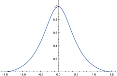
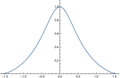
$\kappa=4$
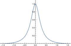
$\kappa=8$

Figure 2: Graphs of the orientation selectivity for purely spatial models of (left column) simple cells in terms of first-order directional derivatives of affine Gaussian kernels, (middle column) simple cells in terms of second-order directional derivatives of affine Gaussian kernels and (right column) complex cells in terms of directional quasi quadrature measures that combine the first- and second-order simple cell responses in a Euclidean way for $C=1/\sqrt{2}$, and shown for different values of the ratio $\kappa$ between the spatial scale parameters in the vertical vs. the horizontal directions. Observe how the degree of orientation selectivity varies strongly depending on the eccentricity $\epsilon=1/\kappa$ of the receptive fields. (top row) Results for $\kappa=1$. (second row) Results for $\kappa=2$. (third row) Results for $\kappa=4$. (bottom row) Results for $\kappa=8$. (Horizontal axes: orientation $\theta\in[-\pi/2,\pi/2]$. Vertical axes: Amplitude of the receptive field response relative to the maximum response obtained for $\theta=0$.)

$$\begin{split}{\cal Q}_{0,spat,norm}L=\sqrt[4]{2}e^{-\frac{1}{\sqrt{2}}}\frac{\left|\cos\theta\right|}{\cos^{2}\theta+\kappa^{2}\sin^{2}\theta}\sqrt{\cos^{2}\theta+\kappa^{2}\sin^{2}\theta\cos^{2}\left(\frac{\sqrt[4]{2}}{\sqrt{\cos^{2}\theta+\kappa^{2}\sin^{2}\theta}}\left(\frac{x_{1}\cos\theta}{\sigma_{1}}+\frac{x_{2}\sin\theta}{\sigma_{1}}\right)+\beta\right)}\end{split}$$ (26)

Figure 3: The expression for the oriented spatial quasi quadrature measure ${\cal Q}_{0,spat,norm}L$ in the purely spatial model (39) of a complex cell, when applied to a sine wave pattern of the form (27), for $\omega=\omega_{\cal Q}$ according to (40).

3.3 Analysis for purely spatial models of receptive fields

For the forthcoming purely spatial analysis, we will analyze the response properties of our spatial models of simple and complex cells to sine wave patterns with angular frequency $\omega$ and orientation $\theta$ of the form

$$f(x_{1},x_{2})=\sin\left(\omega\cos(\theta)\,x_{1}+\omega\sin(\theta)\,x_{2}+\beta\right).$$ (27)

3.3.1 First-order simple cell

Consider a simple cell that is modelled as a first-order scale-normalized derivative of an affine Gaussian kernel (according to (1) for $m=1$), and oriented in the horizontal $x_{1}$-direction (for $\varphi=0$) with spatial scale parameter $\sigma_{1}$ in the horizontal $x_{1}$-direction and spatial scale parameter $\sigma_{2}$ in the vertical $x_{2}$-direction, and thus a spatial covariance matrix of the form $\Sigma_{0}=\operatorname{diag}(\sigma_{1}^{2},\sigma_{2}^{2})$:

$$\begin{split}&T_{0,norm}(x_{1},x_{2};\;\sigma_{1},\sigma_{2})=\end{split}$$

$$\begin{split}&=\frac{\sigma_{1}}{2\pi\sigma_{1}\sigma_{2}}\,\partial_{x_{1}}\left(e^{-x_{1}^{2}/2\sigma_{1}^{2}-x_{2}^{2}/2\sigma_{2}^{2}}\right)\end{split}$$

$$\begin{split}&=-\frac{x_{1}}{2\pi\sigma_{1}^{2}\sigma_{2}}\,e^{-x_{1}^{2}/2\sigma_{1}^{2}-x_{2}^{2}/2\sigma_{2}^{2}}.\end{split}$$ (28)

The corresponding receptive field response is then, after solving the convolution integral in Mathematica,

$$\begin{split}L_{0,norm}(x_{1},x_{2};\;\sigma_{1},\sigma_{2})=\end{split}$$

$$\begin{split}&=\int_{\xi_{1}=-\infty}^{\infty}\int_{\xi_{2}=-\infty}^{\infty}T_{0,norm}(\xi_{1},\xi_{2};\;\sigma_{1},\sigma_{2})\end{split}$$

$$\begin{split}&\phantom{==\int_{\xi_{1}=-\infty}^{\infty}\int_{\xi_{2}=-\infty}^{\infty}}\times f(x_{1}-\xi_{1},x_{2}-\xi_{2})\,d\xi_{1}\xi_{2}\end{split}$$

$$\begin{split}&=\omega\,\sigma_{1}\cos(\theta)\,e^{-\frac{1}{2}\omega^{2}(\sigma_{1}^{2}\cos^{2}\theta+\sigma_{2}^{2}\sin^{2}\theta)}\end{split}$$

$$\begin{split}&\phantom{==}\times\cos\left(\omega\cos(\theta)\,x_{1}+\omega\sin(\theta)\,x_{2}+\beta\right),\end{split}$$ (29)

i.e., a cosine wave with amplitude

$$A_{\varphi}(\theta,\omega;\;\sigma_{1},\sigma_{2})=\omega\,\sigma_{1}\left|\cos\theta\right|\,e^{-\frac{1}{2}\omega^{2}(\sigma_{1}^{2}\cos^{2}\theta+\sigma_{2}^{2}\sin^{2}\theta)}.$$ (30)

If we assume that the receptive field is fixed, then the amplitude of the response will depend strongly on the angular frequency $\omega$ of the sine wave. The value first increases because of the factor $\omega$ and then decreases because of the exponential decrease with $\omega^{2}$.

If we assume that a biological experiment regarding orientation selectivity is carried out in such a way that the angular frequency is varied for each inclination angle $\theta$, and then that the result is for each value of $\theta$ reported for the angular frequency $\hat{\omega}$ that leads to the maximum response, then we can determine this value of $\hat{\omega}$ by differentiating $A_{\varphi}(\theta,\omega;\;\sigma_{1},\sigma_{2})$ with respect to $\omega$ and setting the derivative to zero, which gives:

$$\hat{\omega}_{\varphi}=\frac{1}{\sigma_{1}\sqrt{\cos^{2}\theta+\kappa\sin^{2}\theta}}.$$ (31)

Inserting this values into $A_{\varphi}(\theta,\omega;\;\sigma_{1},\sigma_{2})$, and introducing a scale parameter ratio $\kappa$ such that

$$\sigma_{2}=\kappa\,\sigma_{1},$$ (32)

then gives the following orientation selectivity measure

$$A_{\varphi,max}(\theta,\;\kappa)=\frac{\left|\cos\theta\right|}{\sqrt{e}\sqrt{\cos^{2}\theta+\kappa^{2}\sin^{2}\theta}}.$$ (33)

Note, specifically, that this amplitude measure is independent of the spatial scale parameter $\sigma_{1}$ of the receptive field, which, in turn, is a consequence of the scale-invariant nature of differential expressions in terms of scale-normalized derivatives for scale normalization parameter $\gamma=1$.

The left column in Figure 2 shows the result of plotting the measure $A_{\varphi,max}(\theta;\;\kappa)$ of the orientation selectivity as function of the inclination angle $\theta$ for a few values of the scale parameter ratio $\kappa$, with the values rescaled such that the peak value for each graph is equal to 1. As can be seen from the graphs, the degree of orientation selectivity increases strongly with the value of the spatial scale ratio parameter $\kappa$.

3.3.2 Second-order simple cell

Consider next a simple cell that can be modelled as a second-order scale-normalized derivative of an affine Gaussian kernel (according to (1) for $m=2$), and oriented in the horizontal $x_{1}$-direction (for $\varphi=0$) with spatial scale parameter $\sigma_{1}$ in the horizontal $x_{1}$-direction and spatial scale parameter $\sigma_{2}$ in the vertical $x_{2}$-direction, and thus again with a spatial covariance matrix of the form $\Sigma_{0}=\operatorname{diag}(\sigma_{1}^{2},\sigma_{2}^{2})$:

$$\begin{split}&T_{00,norm}(x_{1},x_{2};\;\sigma_{1},\sigma_{2})=\end{split}$$

$$\begin{split}&=\frac{\sigma_{1}^{2}}{2\pi\sigma_{1}\sigma_{2}}\,\partial_{x_{1}x_{1}}\left(e^{-x_{1}^{2}/2\sigma_{1}^{2}-x_{2}^{2}/2\sigma_{2}^{2}}\right)\end{split}$$

$$\begin{split}&=\frac{(x_{1}^{2}-\sigma_{1}^{2})}{2\pi\sigma_{1}^{3}\sigma_{2}}\,e^{-x_{1}^{2}/2\sigma_{1}^{2}-x_{2}^{2}/2\sigma_{2}^{2}}.\end{split}$$ (34)

The corresponding receptive field response is then, again after solving the convolution integral in Mathematica,

$$\begin{split}L_{00,norm}(x_{1},x_{2};\;\sigma_{1},\sigma_{2})=\end{split}$$

$$\begin{split}&=\int_{\xi_{1}=-\infty}^{\infty}\int_{\xi_{2}=-\infty}^{\infty}T_{00,norm}(\xi_{1},\xi_{2};\;\sigma_{1},\sigma_{2})\end{split}$$

$$\begin{split}&\phantom{==\int_{\xi_{1}=-\infty}^{\infty}\int_{\xi_{2}=-\infty}^{\infty}}\times f(x_{1}-\xi_{1},x_{2}-\xi_{2})\,d\xi_{1}\xi_{2}\end{split}$$

$$\begin{split}&=-\omega^{2}\,\sigma_{1}^{2}\cos^{2}(\theta)\,e^{-\frac{1}{2}\omega^{2}(\sigma_{1}^{2}\cos^{2}\theta+\sigma_{2}^{2}\sin^{2}\theta)}\end{split}$$

$$\begin{split}&\phantom{==}\times\sin\left(\omega\cos(\theta)\,x_{1}+\omega\sin(\theta)\,x_{2}+\beta\right),\end{split}$$ (35)

i.e., a sine wave with amplitude

$$A_{\varphi\varphi}(\theta,\omega;\;\sigma_{1},\sigma_{2})=\omega^{2}\,\sigma_{1}^{2}\cos^{2}(\theta)\,e^{-\frac{1}{2}\omega^{2}(\sigma_{1}^{2}\cos^{2}\theta+\sigma_{2}^{2}\sin^{2}\theta)}.$$ (36)

Again, also this expression first increases and then increases with the angular frequency $\omega$. Selecting again the value of $\hat{\omega}$ at which the amplitude receptive field response assumes its maximum over $\omega$ gives

$$\hat{\omega}_{\varphi\varphi}=\frac{\sqrt{2}}{\sigma_{1}\sqrt{\cos^{2}\theta+\kappa\sin^{2}\theta}},$$ (37)

and implies that the maximum amplitude over spatial scales as function of the inclination angle $\theta$ and the scale parameter ratio $\kappa$ can be written

$$A_{\varphi\varphi,max}(\theta;\;\kappa)=\frac{\cos^{2}\theta}{\sqrt{e}\left(\cos^{2}\theta+\kappa^{2}\sin^{2}\theta\right)}.$$ (38)

Again, this amplitude measure is also independent of the spatial scale parameter $\sigma_{1}$ of the receptive field, because of the scale-invariant property of scale-normalized derivatives, when the scale normalization parameter $\gamma$ is chosen as $\gamma=1$.

The middle column in Figure 2 shows the result of plotting the measure $A_{\varphi\varphi,max}(\theta;\;\kappa)$ of the orientation selectivity as function of the inclination angle $\theta$ for a few values of the scale parameter ratio $\kappa$, with the values rescaled such that the peak value for each graph is equal to 1. Again, the degree of orientation selectivity increases strongly with the value of $\kappa$, as for the first-order model of a simple cell.

3.3.3 Complex cell

To model the spatial response of a complex cell according to the spatial quasi quadrature measure (10), we combine the responses of the first- and second-order simple cells for $\Gamma=0$:

$${\cal Q}_{0,spat,norm}L=\sqrt{L_{0,norm}^{2}+C_{\varphi}\,L_{00,norm}^{2}},$$ (39)

with $L_{0,norm}$ according to (LABEL:eq-L0-pure-spat-anal) and $L_{00,norm}$ according to (LABEL:eq-L00-pure-spat-anal). Choosing the angular frequency $\hat{\omega}$ as the geometric average of the angular frequencies for which the first- and second-order components of this entity assume their maxima over angular frequencies, respectively,

$$\hat{\omega}_{\cal Q}=\sqrt{\hat{\omega}_{\varphi}\,\hat{\omega}_{\varphi\varphi}}=\frac{\sqrt[4]{2}}{\sigma_{1}\sqrt{\cos^{2}\theta+\kappa^{2}\sin^{2}\theta}},$$ (40)

with $\hat{\omega}_{\varphi}$ according to (31) and $\hat{\omega}_{\varphi\varphi}$ according to (37). Again letting $\sigma_{1}=\kappa\,\sigma_{1}$, and setting the relative weight between first- and second-order information to $C_{\varphi}=1/\sqrt{2}$ according to (Lindeberg 2018), gives the expression according to Equation (26) in Figure 3.

For inclination angle $\theta=0$, that measure is spatially constant, in agreement with previous work on closely related isotropic purely spatial isotropic quasi quadrature measures (Lindeberg 2018). Then, the spatial phase dependency increases with increasing values of the inclination angle $\theta$. To select a single representative of those differing representations, let us choose the geometric average of the extreme values, which then assumes the form

$$A_{{\cal Q},spat}(\theta;\;\kappa)=\frac{\sqrt[4]{2}\,\left|\cos\theta\right|^{3}}{\sqrt{e}\left(\cos^{2}\theta+\kappa^{2}\sin^{2}\theta\right)^{3/4}}.$$ (41)

The right column in Figure 2 shows the result of plotting the measure $A_{{\cal Q},spat}(\theta;\;\kappa)$ of the orientation selectivity as function of the inclination angle $\theta$ for a few values of the scale parameter ratio $\kappa$, with the values rescaled such that the peak value for each graph is equal to 1. As can be seen from the graphs, the degree of orientation selectivity increases strongly with the value of $\kappa$ also for this model of a complex cell, and in a qualitatively similar way as for the simple cell models.

	First-order first-order simple cell	Second-order second-order simple cell	Complex cell
$\kappa=1$
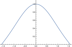
$\kappa=2$
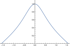
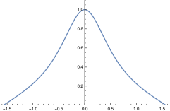
$\kappa=4$
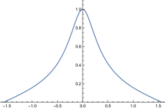
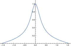
$\kappa=8$

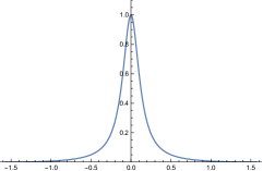
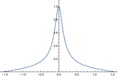
Figure 4: Graphs of the orientation selectivity for space-time separable spatio-temporal models of (left column) simple cells in terms of first-order directional derivatives of affine Gaussian kernels combined with first-order temporal derivatives of temporal Gaussian kernels, (middle column) simple cells in terms of second-order directional derivatives of affine Gaussian kernels combined with second-order temporal derivatives of temporal Gaussian kernels and (right column) complex cells in terms of directional quasi quadrature measures that combine the first- and second-order simple cell responses in a Euclidean way for $C_{\varphi}=1/\sqrt{2}$, and $C_{t}=1/\sqrt{2}$ shown for different values of the ratio $\kappa$ between the spatial scale parameters in the vertical vs. the horizontal directions. Observe how the degree of orientation selectivity varies strongly depending on the eccentricity $\epsilon=1/\kappa$ of the receptive fields. (top row) Results for $\kappa=1$. (second row) Results for $\kappa=2$. (third row) Results for $\kappa=4$. (bottom row) Results for $\kappa=8$. (Horizontal axes: orientation $\theta\in[-\pi/2,\pi/2]$. Vertical axes: Amplitude of the receptive field response relative to the maximum response obtained for $\theta=0$.)

3.4 Analysis for space-time separable models of spatio-temporal receptive fields

To investigate the directional selectivity of our spatio-temporal models for simple and complex cells, we will analyze their response properties to a moving sine wave of the form

$$f(x_{1},x_{2},t)=\\ =\sin\left(\omega\cos(\theta)\,(x_{1}-u_{1}t)+\omega\sin(\theta)\,(x_{2}-u_{2}t)+\beta\right),$$ (42)

where we choose the velocity vector $(u_{1},u_{2})^{T}$ parallel to the inclination angle $\theta$ of the grating according to $(u_{1},u_{2})^{T}=(u\cos\theta,u\sin\theta)^{T}$, which, in turn, implies the form

$$f(x_{1},x_{2},t)=\\ =\sin\left(\omega\cos(\theta)\,x_{1}+\omega\sin(\theta)\,x_{2}-u\,t+\beta\right).$$ (43)

Let us initially perform such an analysis for space-time separable models of simple and complex cells, in which the velocity vector $v$ in the spatio-temporal receptive field models is set to zero.

For simplicity, we initially perform the theoretical analysis for non-causal spatio-temporal receptive field models, where the temporal components are given as scale-normalized temporal derivatives of 1-D temporal Gaussian kernels.

In the following, we will name our models of spatio-temporal receptive fields according to the orders of differentiation with respect to space and time.

3.4.1 First-order first-order simple cell

Consider a space-time separable receptive field corresponding to a first-order scale-normalized Gaussian derivative with scale parameter $\sigma_{1}$ in the horizontal $x_{1}$-direction, a zero-order Gaussian kernel with scale parameter $\sigma_{2}$ in the vertical $x_{2}$-direction, and a first-order scale-normalized Gaussian derivative with scale parameter $\sigma_{t}$ in the temporal direction, corresponding to $\varphi=0$, $v=0$, $\Sigma_{0}=\operatorname{diag}(\sigma_{1}^{2},\sigma_{2}^{2})$, $m=1$ and $n=1$ in (2.3):

$$\begin{split}&T_{0,t,norm}(x_{1},x_{2},t;\;\sigma_{1},\sigma_{2},\sigma_{t})=\end{split}$$

$$\begin{split}&=\frac{\sigma_{1}\sigma_{t}}{(2\pi)^{3/2}\,\sigma_{1}\sigma_{2}\sigma_{t}}\,\partial_{x_{1}}\partial_{t}\left(e^{-x_{1}^{2}/2\sigma_{1}^{2}-x_{2}^{2}/2\sigma_{2}^{2}-t^{2}/2\sigma_{t}^{2}}\right)\end{split}$$

$$\begin{split}&=\frac{x_{1}t}{(2\pi)^{3/2}\,\sigma_{1}^{2}\sigma_{2}\sigma_{t}^{2}}\,e^{-x_{1}^{2}/2\sigma_{1}^{2}-x_{2}^{2}/2\sigma_{2}^{2}-t^{2}/2\sigma_{t}^{2}}.\end{split}$$ (44)

The corresponding receptive field response is then, after solving the convolution integral in Mathematica,

$$\begin{split}L_{0,t,norm}(x_{1},x_{2},t;\;\sigma_{1},\sigma_{2},\sigma_{t})=\end{split}$$

$$\begin{split}&=\int_{\xi_{1}=-\infty}^{\infty}\int_{\xi_{2}=-\infty}^{\infty}\int_{\zeta=-\infty}^{\infty}T_{0,t,norm}(\xi_{1},\xi_{2},\zeta;\;\sigma_{1},\sigma_{2},\sigma_{t})\end{split}$$

$$\begin{split}&\phantom{==\int_{\xi_{1}=-\infty}^{\infty}\int_{\xi_{2}=-\infty}^{\infty}}\times f(x_{1}-\xi_{1},x_{2}-\xi_{2},t-\zeta)\,d\xi_{1}\xi_{2}d\zeta\end{split}$$

$$\begin{split}&=\omega^{2}\,\sigma_{1}\,\sigma_{t}\,u\cos(\theta)\,e^{-\frac{1}{2}\omega^{2}(\sigma_{1}^{2}\cos^{2}\theta+\sigma_{2}^{2}\sin^{2}\theta+\sigma_{t}^{2}u^{2})}\end{split}$$

$$\begin{split}&\phantom{==}\times\sin\left(\omega\cos(\theta)\,x_{1}+\omega\sin(\theta)\,x_{2}-u\,t+\beta\right),\end{split}$$ (45)

i.e., a sine wave with amplitude

$$A_{\varphi,t}(\theta,u,\omega;\;\sigma_{1},\sigma_{2},\sigma_{t})=\\ =\omega^{2}\,\sigma_{1}\,\sigma_{t}\,u\cos(\theta)\,e^{-\frac{1}{2}\omega^{2}(\sigma_{1}^{2}\cos^{2}\theta+\sigma_{2}^{2}\sin^{2}\theta+\sigma_{t}^{2}u^{2})}.$$ (46)

This expression first increases and then decreases with respect to both the angular frequency $\omega$ and the velocity $u$ of the sine wave. Selecting the values of $\hat{\omega}$ and $\hat{u}$ at which this expression assumes its maximum over $\omega$ and $u$

$$\hat{\omega}_{\varphi,t}=\frac{1}{\sigma_{1}\sqrt{\cos^{2}\theta+\kappa\sin^{2}\theta}},$$ (47)

$$\hat{u}_{\varphi,t}=\frac{\sigma_{1}}{\sigma_{t}}\sqrt{\cos^{2}\theta+\kappa\sin^{2}\theta},$$ (48)

and again reparameterizing the other spatial scale parameter $\sigma_{2}$ as $\sigma_{2}=\kappa\,\sigma_{1}$, gives that the maximum amplitude measure over spatial and temporal scales is

$$A_{\varphi,t,max}(\theta;\;\kappa)=\frac{\cos\theta}{e\sqrt{\cos^{2}\theta+\kappa^{2}\sin^{2}\theta}}.$$ (49)

Note that again this directional selectivity measure is independent of the spatial scale parameter $\sigma_{1}$ as well as independent of the temporal scale parameter $\sigma_{t}$, because of the scale-invariant property of scale-normalized derivatives for scale normalization power $\gamma=1$.

The left column in Figure 4 shows the result of plotting the measure $A_{\varphi,t,max}(\theta;\;\kappa)$ of the orientation selectivity as function of the inclination angle $\theta$ for a few values of the scale parameter ratio $\kappa$, with the values rescaled such that the peak value for each graph is equal to 1. As we can see from the graphs, as for the previous purely spatial model of the receptive fields, the degree of orientation selectivity increases strongly with the value of $\kappa$.

3.4.2 First-order second-order simple cell

Consider a space-time separable receptive field corresponding to a first-order scale-normalized Gaussian derivative with scale parameter $\sigma_{1}$ in the horizontal $x_{1}$-direction, a zero-order Gaussian kernel with scale parameter $\sigma_{2}$ in the vertical $x_{2}$-direction, and a second-order scale-normalized Gaussian derivative with scale parameter $\sigma_{t}$ in the temporal direction, corresponding to $\varphi=0$, $v=0$, $\Sigma_{0}=\operatorname{diag}(\sigma_{1}^{2},\sigma_{2}^{2})$, $m=1$ and $n=2$ in (2.3):

$$\begin{split}&T_{0,tt,norm}(x_{1},x_{2},t;\;\sigma_{1},\sigma_{2},\sigma_{t})=\end{split}$$

$$\begin{split}&=\frac{\sigma_{1}\sigma_{t}^{2}}{(2\pi)^{3/2}\,\sigma_{1}\sigma_{2}\sigma_{t}}\,\partial_{x_{1}}\partial_{tt}\left(e^{-x_{1}^{2}/2\sigma_{1}^{2}-x_{2}^{2}/2\sigma_{2}^{2}-t^{2}/2\sigma_{t}^{2}}\right)\end{split}$$

$$\begin{split}&=-\frac{x_{1}(t^{2}-\sigma_{t}^{2})}{(2\pi)^{3/2}\,\sigma_{1}^{2}\sigma_{2}\sigma_{t}^{3}}\,e^{-x_{1}^{2}/2\sigma_{1}^{2}-x_{2}^{2}/2\sigma_{2}^{2}-t^{2}/2\sigma_{t}^{2}}.\end{split}$$ (50)

The corresponding receptive field response is then, after solving the convolution integral in Mathematica,

$$\begin{split}L_{0,tt,norm}(x_{1},x_{2},t;\;\sigma_{1},\sigma_{2},\sigma_{t})=\end{split}$$

$$\begin{split}&=\int_{\xi_{1}=-\infty}^{\infty}\int_{\xi_{2}=-\infty}^{\infty}\int_{\zeta=-\infty}^{\infty}T_{0,tt,norm}(\xi_{1},\xi_{2},\zeta;\;\sigma_{1},\sigma_{2},\sigma_{t})\end{split}$$

$$\begin{split}&\phantom{==\int_{\xi_{1}=-\infty}^{\infty}\int_{\xi_{2}=-\infty}^{\infty}}\times f(x_{1}-\xi_{1},x_{2}-\xi_{2},t-\zeta)\,d\xi_{1}\xi_{2}d\zeta\end{split}$$

$$\begin{split}&=-\omega^{3}\,\sigma_{1}\,\sigma_{t}^{2}\,u^{2}\cos(\theta)\,e^{-\frac{1}{2}\omega^{2}(\sigma_{1}^{2}\cos^{2}\theta+\sigma_{2}^{2}\sin^{2}\theta+\sigma_{t}^{2}u^{2})}\end{split}$$

$$\begin{split}&\phantom{==}\times\cos\left(\omega\cos(\theta)\,x_{1}+\omega\sin(\theta)\,x_{2}-u\,t+\beta\right),\end{split}$$ (51)

i.e., a cosine wave with amplitude

$$A_{\varphi,tt}(\theta,u,\omega;\;\sigma_{1},\sigma_{2},\sigma_{t})=\\ =\omega^{3}\,\sigma_{1}\,\sigma_{t}^{2}\,u^{2}\cos(\theta)\,e^{-\frac{1}{2}\omega^{2}(\sigma_{1}^{2}\cos^{2}\theta+\sigma_{2}^{2}\sin^{2}\theta+\sigma_{t}^{2}u^{2})}.$$ (52)

This entity assumes its maximum over the angular frequency $\omega$ and the image velocity $u$ at

$$\hat{\omega}_{\varphi,tt}=\frac{1}{\sigma_{1}\sqrt{\cos^{2}\theta+\kappa\sin^{2}\theta}},$$ (53)

$$\hat{u}_{\varphi,tt}=\frac{\sqrt{2}\sigma_{1}}{\sigma_{t}}\sqrt{\cos^{2}\theta+\kappa\sin^{2}\theta},$$ (54)

and again reparameterizing the other spatial scale parameter $\sigma_{2}$ as $\sigma_{2}=\kappa\,\sigma_{1}$, gives that the maximum amplitude measure over spatial and temporal scales is

$$A_{\varphi,tt,max}(\theta;\;\kappa)=\frac{2\cos\theta}{e^{3/2}\sqrt{\cos^{2}\theta+\kappa^{2}\sin^{2}\theta}},$$ (55)

i.e., of a similar form as the previous measure $A_{\varphi,tt,max}(\theta;\;\kappa)$, while being multiplied by another constant.

3.4.3 Second-order first-order simple cell

Consider a space-time separable receptive field corresponding to a second-order scale-normalized Gaussian derivative with scale parameter $\sigma_{1}$ in the horizontal $x_{1}$-direction, a zero-order Gaussian kernel with scale parameter $\sigma_{2}$ in the vertical $x_{2}$-direction, and a first-order scale-normalized Gaussian derivative with scale parameter $\sigma_{t}$ in the temporal direction, corresponding to $\varphi=0$, $v=0$, $\Sigma_{0}=\operatorname{diag}(\sigma_{1}^{2},\sigma_{2}^{2})$, $m=2$ and $n=1$ in (2.3):

$$\begin{split}&T_{00,t,norm}(x_{1},x_{2},t;\;\sigma_{1},\sigma_{2},\sigma_{t})=\end{split}$$

$$\begin{split}&=\frac{\sigma_{1}^{2}\sigma_{t}}{(2\pi)^{3/2}\,\sigma_{1}\sigma_{2}\sigma_{t}}\,\partial_{x_{1}x_{1}}\partial_{t}\left(e^{-x_{1}^{2}/2\sigma_{1}^{2}-x_{2}^{2}/2\sigma_{2}^{2}-t^{2}/2\sigma_{t}^{2}}\right)\end{split}$$

$$\begin{split}&=-\frac{(x_{1}^{2}-\sigma_{1}^{2})t}{(2\pi)^{3/2}\,\sigma_{1}^{3}\sigma_{2}\sigma_{t}^{2}}\,e^{-x_{1}^{2}/2\sigma_{1}^{2}-x_{2}^{2}/2\sigma_{2}^{2}-t^{2}/2\sigma_{t}^{2}}.\end{split}$$ (56)

The corresponding receptive field response is then, after solving the convolution integral in Mathematica,

$$\begin{split}L_{00,t,norm}(x_{1},x_{2},t;\;\sigma_{1},\sigma_{2},\sigma_{t})=\end{split}$$

$$\begin{split}&=\int_{\xi_{1}=-\infty}^{\infty}\int_{\xi_{2}=-\infty}^{\infty}\int_{\zeta=-\infty}^{\infty}T_{00,t,norm}(\xi_{1},\xi_{2},\zeta;\;\sigma_{1},\sigma_{2},\sigma_{t})\end{split}$$

$$\begin{split}&\phantom{==\int_{\xi_{1}=-\infty}^{\infty}\int_{\xi_{2}=-\infty}^{\infty}}\times f(x_{1}-\xi_{1},x_{2}-\xi_{2},t-\zeta)\,d\xi_{1}\xi_{2}d\zeta\end{split}$$

$$\begin{split}&=-\omega^{3}\,\sigma_{1}^{2}\,\sigma_{t}\,u\cos^{2}(\theta)\,e^{-\frac{1}{2}\omega^{2}(\sigma_{1}^{2}\cos^{2}\theta+\sigma_{2}^{2}\sin^{2}\theta+\sigma_{t}^{2}u^{2})}\end{split}$$

$$\begin{split}&\phantom{==}\times\cos\left(\omega\cos(\theta)\,x_{1}+\omega\sin(\theta)\,x_{2}-u\,t+\beta\right),\end{split}$$ (57)

i.e., a cosine wave with amplitude

$$A_{\varphi\varphi,t}(\theta,u,\omega;\;\sigma_{1},\sigma_{2},\sigma_{t})=\\ =\omega^{3}\,\sigma_{1}^{2}\,\sigma_{t}\,u\cos^{2}(\theta)\,e^{-\frac{1}{2}\omega^{2}(\sigma_{1}^{2}\cos^{2}\theta+\sigma_{2}^{2}\sin^{2}\theta+\sigma_{t}^{2}u^{2})}.$$ (58)

This entity assumes its maximum over spatial scale $\sigma_{1}$ and over temporal scale $\sigma_{t}$ at

$$\hat{\omega}_{\varphi\varphi,t}=\frac{\sqrt{2}}{\sigma_{1}\sqrt{\cos^{2}\theta+\kappa\sin^{2}\theta}},$$ (59)

$$\hat{u}_{\varphi\varphi,t}=\frac{\sigma_{1}}{\sqrt{2}\sigma_{t}}\sqrt{\cos^{2}\theta+\kappa\sin^{2}\theta},$$ (60)

and again reparameterizing the other spatial scale parameter $\sigma_{2}$ as $\sigma_{2}=\kappa\,\sigma_{1}$, gives that the maximum amplitude measure over spatial and temporal scales is

$$A_{\varphi\varphi,t,max}(\theta;\;\kappa)=\frac{2\cos^{2}\theta}{e^{3/2}\left(\cos^{2}\theta+\kappa^{2}\sin^{2}\theta\right)}.$$ (61)

3.4.4 Second-order second-order simple cell

Consider a space-time separable receptive field corresponding to a second-order scale-normalized Gaussian derivative with scale parameter $\sigma_{1}$ in the horizontal $x_{1}$-direction, a zero-order Gaussian kernel with scale parameter $\sigma_{2}$ in the vertical $x_{2}$-direction, and a second-order scale-normalized Gaussian derivative with scale parameter $\sigma_{t}$ in the temporal direction, corresponding to $\varphi=0$, $v=0$, $\Sigma_{0}=\operatorname{diag}(\sigma_{1}^{2},\sigma_{2}^{2})$, $m=2$ and $n=2$ in (2.3):

$$\begin{split}&T_{00,tt,norm}(x_{1},x_{2},t;\;\sigma_{1},\sigma_{2},\sigma_{t})=\end{split}$$

$$\begin{split}&=\frac{\sigma_{1}^{2}\sigma_{t}^{2}}{(2\pi)^{3/2}\,\sigma_{1}\sigma_{2}\sigma_{t}}\,\partial_{x_{1}x_{1}}\partial_{tt}\left(e^{-x_{1}^{2}/2\sigma_{1}^{2}-x_{2}^{2}/2\sigma_{2}^{2}-t^{2}/2\sigma_{t}^{2}}\right)\end{split}$$

$$\begin{split}&=\frac{(x_{1}^{2}-\sigma_{1}^{2})(t^{2}-\sigma_{t}^{2})}{(2\pi)^{3/2}\,\sigma_{1}^{3}\sigma_{2}\sigma_{t}^{3}}\,e^{-x_{1}^{2}/2\sigma_{1}^{2}-x_{2}^{2}/2\sigma_{2}^{2}-t^{2}/2\sigma_{t}^{2}}.\end{split}$$ (62)

The corresponding receptive field response is then, after solving the convolution integral in Mathematica,

$$\begin{split}L_{00,tt,norm}(x_{1},x_{2},t;\;\sigma_{1},\sigma_{2},\sigma_{t})=\end{split}$$

$$\begin{split}&=\int_{\xi_{1}=-\infty}^{\infty}\int_{\xi_{2}=-\infty}^{\infty}\int_{\zeta=-\infty}^{\infty}T_{00,tt,norm}(\xi_{1},\xi_{2},\zeta;\;\sigma_{1},\sigma_{2},\sigma_{t})\end{split}$$

$$\begin{split}&\phantom{==\int_{\xi_{1}=-\infty}^{\infty}\int_{\xi_{2}=-\infty}^{\infty}}\times f(x_{1}-\xi_{1},x_{2}-\xi_{2},t-\zeta)\,d\xi_{1}\xi_{2}d\zeta\end{split}$$

$$\begin{split}&=\omega^{4}\,\sigma_{1}^{2}\,\sigma_{t}^{2}\,u^{2}\cos^{2}(\theta)\,e^{-\frac{1}{2}\omega^{2}(\sigma_{1}^{2}\cos^{2}\theta+\sigma_{2}^{2}\sin^{2}\theta+\sigma_{t}^{2}u^{2})}\end{split}$$

$$\begin{split}&\phantom{==}\times\sin\left(\omega\cos(\theta)\,x_{1}+\omega\sin(\theta)\,x_{2}-u\,t+\beta\right),\end{split}$$ (63)

i.e., a sine wave with amplitude

$$A_{\varphi\varphi,tt}(\theta,u,\omega;\;\sigma_{1},\sigma_{2},\sigma_{t})=\\ =\omega^{4}\,\sigma_{1}^{2}\,\sigma_{t}^{2}\,u^{2}\cos^{2}(\theta)\,e^{-\frac{1}{2}\omega^{2}(\sigma_{1}^{2}\cos^{2}\theta+\sigma_{2}^{2}\sin^{2}\theta+\sigma_{t}^{2}u^{2})}.$$ (64)

This entity assumes its maximum over spatial scale $\sigma_{1}$ and over temporal scale $\sigma_{t}$ at

$$\hat{\omega}_{\varphi\varphi,tt}=\frac{\sqrt{2}}{\sigma_{1}\sqrt{\cos^{2}\theta+\kappa\sin^{2}\theta}},$$ (65)

$$\hat{u}_{\varphi\varphi,tt}=\frac{\sigma_{1}}{\sigma_{t}}\sqrt{\cos^{2}\theta+\kappa\sin^{2}\theta},$$ (66)

and again reparameterizing the other spatial scale parameter $\sigma_{2}$ as $\sigma_{2}=\kappa\,\sigma_{1}$, gives that the maximum amplitude measure over spatial and temporal scales is

$$A_{\varphi\varphi,tt,max}(\theta;\;\kappa)=\frac{4\cos^{2}\theta}{e^{2}\left(\cos^{2}\theta+\kappa^{2}\sin^{2}\theta\right)}.$$ (67)

The middle column in Figure 4 shows the result of plotting the measure $A_{\varphi\varphi,tt,max}(\theta;\;\kappa)$ of the orientation selectivity as function of the inclination angle $\theta$ for a few values of the scale parameter ratio $\kappa$, with the values rescaled such that the peak value is equal to 1. Again, the degree of orientation selectivity increases strongly with the value of $\kappa$, as for the first-order first-order model of a simple cell.

3.4.5 Complex cell

To model the spatio-temporal response of a complex cell according to the directional sensitive spatio-temporal quasi quadrature measure (2.3) based on space-time separable spatio-temporal receptive fields, we combine the responses of the first-order first-order simple cell (LABEL:eq-L0t-space-time-sep-anal), the first-order second-order cell (LABEL:eq-L0tt-space-time-sep-anal), the second-order first-order simple cell (LABEL:eq-L00t-space-time-sep-anal) and the second-order second order cell (LABEL:eq-L00tt-space-time-sep-anal) for $v=0$, $\Gamma_{\varphi}=0$ and $\Gamma_{t}=0$ according to

$$\begin{split}&({\cal Q}_{0,sep,norm}L)^{2}\end{split}$$

$$\begin{split}&=L_{0,t,norm}^{2}+C_{\varphi}\,L_{00,t,norm}^{2}+\end{split}$$

$$\begin{split}&\phantom{=}+C_{t}\left(L_{0,tt,norm}^{2}+C_{\varphi}\,L_{00,tt,norm}^{2}\right).\end{split}$$ (68)

Selecting the angular frequency $\hat{\omega}$ as the geometric average of the angular frequencies where the above spatio-temporal simple cell models assume their maximum amplitude responses over spatial scales

$$\hat{\omega}_{\cal Q}=\sqrt{\hat{\omega}_{\varphi,t}\,\hat{\omega}_{\varphi,tt}\,\hat{\omega}_{\varphi\varphi,t}\,\hat{\omega}_{\varphi\varphi,tt}}=\frac{\sqrt[4]{2}}{\sigma_{1}\sqrt{\cos^{2}\theta+\kappa\sin^{2}\theta}},$$ (69)

and selecting the image velocity $\hat{u}$ of the sine wave as the geometric average of the image velocities where the above spatio-temporal simple cell models assume their maximum amplitude responses over image velocities

$$\hat{u}_{\cal Q}=\sqrt{\hat{u}_{\varphi,t}\,\hat{u}_{\varphi,tt}\,\hat{u}_{\varphi\varphi,t}\,\hat{u}_{\varphi\varphi,tt}}=\frac{\sigma_{1}}{\sigma_{t}}\sqrt{\cos^{2}\theta+\kappa\sin^{2}\theta},$$ (70)

as well as choosing the spatial and temporal weighting factors $C_{\varphi}$ and $C_{t}$ between first- and second-order information as $C_{\varphi}=1/\sqrt{2}$ and $C_{t}=1/\sqrt{2}$ according to (Lindeberg 2018), then implies that the spatio-temporal quasi quadrature measure assumes the form

$$A_{{\cal Q},sep}(\theta;\;\kappa)=\frac{e^{-\sqrt{2}}\left|\cos\theta\right|\,\sqrt{2+\kappa^{2}+(2-\kappa^{2})\cos 2\theta}}{\cos^{2}\theta+\kappa^{2}\sin^{2}\theta}.$$ (71)

Note that this expression is independent of both the spatial scale parameter $\sigma_{1}$ and the temporal scale parameter $\sigma_{t}$, because of the scale-invariant properties of scale-normalized derivatives for scale normalization parameter $\gamma=1$. Moreover, this expression is also independent of the phase of the signal, as determined by the spatial coordinates $x_{1}$ and $x_{2}$, the time moment $t$ and the phase angle $\beta$.

The right column in Figure 4 shows the result of plotting the measure $A_{{\cal Q},sep}(\theta;\;\kappa)$ of the orientation selectivity as function of the inclination angle $\theta$ for a few values of the scale parameter ratio $\kappa$, with the values rescaled such that the peak value for each graph is equal to 1. As can be seen from the graphs, the degree of orientation selectivity increases strongly with the value of $\kappa$ also for this spatio-temporal model of a complex cell, and in a qualitatively similar way as for the simple cell models, regarding both the purely spatial as well as the joint spatio-temporal models of the simple cells.

	First-order first-order simple cell	Second-order second-order simple cell	Complex cell
$\kappa=1$
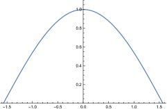
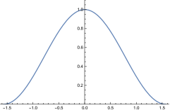
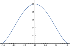
$\kappa=2$
$\kappa=4$
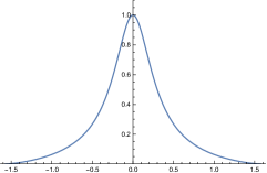
$\kappa=8$

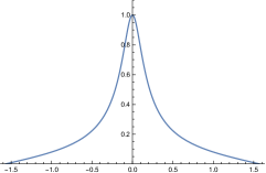
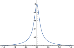
Figure 5: Graphs of the orientation selectivity for velocity-adapted spatio-temporal models of (left column) simple cells in terms of first-order directional derivatives of affine Gaussian kernels combined with zero-order temporal Gaussian kernels, (middle column) simple cells in terms of second-order directional derivatives of affine Gaussian kernels combined with zero-order temporal Gaussian kernels and (right column) complex cells in terms of directional quasi quadrature measures that combine the first- and second-order simple cell responses in a Euclidean way for $C_{\varphi}=1/\sqrt{2}$ shown for different values of the ratio $\kappa$ between the spatial scale parameters in the vertical vs. the horizontal directions. Observe how the degree of orientation selectivity varies strongly depending on the eccentricity $\epsilon=1/\kappa$ of the receptive fields. (top row) Results for $\kappa=1$. (second row) Results for $\kappa=2$. (third row) Results for $\kappa=4$. (bottom row) Results for $\kappa=8$. (Horizontal axes: orientation $\theta\in[-\pi/2,\pi/2]$. Vertical axes: Amplitude of the receptive field response relative to the maximum response obtained for $\theta=0$.)

$$\begin{split}{\cal Q}_{0,vel,norm}L=\sqrt[4]{2}\,e^{-\frac{1}{\sqrt{2}}}\frac{\left|\cos\theta\right|}{\cos^{2}\theta+\kappa^{2}\sin^{2}\theta}\sqrt{\cos^{2}\theta+\kappa^{2}\sin^{2}\theta\,\cos^{2}\left(\frac{2^{3/4}(\cos(\theta)\,(x_{1}-vt)+\sin(\theta)\,x_{2})}{\sigma_{1}\sqrt{1+\kappa^{2}-\left(\kappa^{2}-1\right)\cos 2\theta}}+\beta\right)}\end{split}$$ (72)

Figure 6: The expression for the oriented spatio-temporal quasi quadrature measure ${\cal Q}_{0,vel,norm}L$ in the velocity-adapted spatio-temporal model (23) of a complex cell, when applied to a sine wave pattern of the form (73), for $\omega=\omega_{\cal Q}$ according to (87) and $u=u_{\cal Q}$ according to (88).

3.5 Analysis for velocity-adapted spatio-temporal models of receptive fields

Similar to previous section, we will again analyze the response properties of spatio-temporal receptive fields to a moving sine wave of the form (43)

$$f(x_{1},x_{2},t)=\\ =\sin\left(\omega\cos(\theta)\,x_{1}+\omega\sin(\theta)\,x_{2}-u\,t+\beta\right).$$ (73)

Based on the observation that the response properties of temporal derivatives will be zero, if the velocity $v$ of the spatio-temporal receptive field is adapted to the velocity $u$ of the moving sine wave, we will study the case when the temporal order of differentiation $n$ is zero.

3.5.1 First-order simple cell

Consider a velocity-adapted receptive field corresponding to a first-order scale-normalized Gaussian derivative with scale parameter $\sigma_{1}$ and velocity $v$ in the horizontal $x_{1}$-direction, a zero-order Gaussian kernel with scale parameter $\sigma_{2}$ in the vertical $x_{2}$-direction, and a zero-order Gaussian derivative with scale parameter $\sigma_{t}$ in the temporal direction, corresponding to $\varphi=0$, $v=0$, $\Sigma_{0}=\operatorname{diag}(\sigma_{1}^{2},\sigma_{2}^{2})$, $m=1$ and $n=0$ in (2.3):

$$\begin{split}&T_{0,norm}(x_{1},x_{2},t;\;\sigma_{1},\sigma_{2},\sigma_{t})=\end{split}$$

$$\begin{split}&=\frac{\sigma_{1}}{(2\pi)^{3/2}\,\sigma_{1}\sigma_{2}\sigma_{t}}\,\partial_{x_{1}}\left.\left(e^{-x_{1}^{2}/2\sigma_{1}^{2}-x_{2}^{2}/2\sigma_{2}^{2}-t^{2}/2\sigma_{t}^{2}}\right)\right|_{x_{1}\rightarrow x_{1}-vt}\end{split}$$

$$\begin{split}&=\frac{(x_{1}-vt)}{(2\pi)^{3/2}\,\sigma_{1}^{2}\sigma_{2}\sigma_{t}}\,e^{-(x_{1}-vt)^{2}/2\sigma_{1}^{2}-x_{2}^{2}/2\sigma_{2}^{2}-t^{2}/2\sigma_{t}^{2}}.\end{split}$$ (74)

The corresponding receptive field response is then, after solving the convolution integral in Mathematica,

$$\begin{split}L_{0,norm}(x_{1},x_{2},t;\;\sigma_{1},\sigma_{2},\sigma_{t})=\end{split}$$

$$\begin{split}&=\int_{\xi_{1}=-\infty}^{\infty}\int_{\xi_{2}=-\infty}^{\infty}\int_{\zeta=-\infty}^{\infty}T_{0,norm}(\xi_{1},\xi_{2},\zeta;\;\sigma_{1},\sigma_{2},\sigma_{t})\end{split}$$

$$\begin{split}&\phantom{==\int_{\xi_{1}=-\infty}^{\infty}\int_{\xi_{2}=-\infty}^{\infty}}\times f(x_{1}-\xi_{1},x_{2}-\xi_{2},t-\zeta)\,d\xi_{1}\xi_{2}d\zeta\end{split}$$

$$\begin{split}&=\omega\,\sigma_{1}\cos\theta\,\end{split}$$

$$\begin{split}&\phantom{==}\times e^{-\frac{\omega^{2}}{2}\left(\left(\sigma_{1}^{2}+\sigma_{t}^{2}v^{2}\right)\cos^{2}(\theta)+\sigma_{2}^{2}\sin^{2}\theta-2\sigma_{t}^{2}uv\cos\theta+\sigma_{t}^{2}u^{2}\right)}\end{split}$$

$$\begin{split}&\phantom{==}\times\cos\left(\cos(\theta)\,x_{1}+\sin(\theta)\,x_{2}-\omega u\,t+\beta\right),\end{split}$$ (75)

i.e., a cosine wave with amplitude

$$\begin{split}&A_{\varphi}(\theta,u,\omega;\;\sigma_{1},\sigma_{2},\sigma_{t})=\end{split}$$

$$\begin{split}&=\omega\,\sigma_{1}\cos\theta\,\end{split}$$

$$\begin{split}&\phantom{==}\times e^{-\frac{\omega^{2}}{2}\left(\cos^{2}\theta\left(\sigma_{1}^{2}+\sigma_{t}^{2}v^{2}\right)+\sigma_{2}^{2}\sin^{2}\theta-2\sigma_{t}^{2}uv\cos\theta+\sigma_{t}^{2}u^{2}\right)}.\end{split}$$ (76)

Assume that a biological experiment regarding the response properties of the receptive field is performed by varying both the angular frequency $\omega$ and the image velocity $u$ to get the maximum value of the response over these parameters. Differentiating the amplitude $A_{\varphi}$ with respect to $\omega$ and $u$ and setting these derivative to zero then gives

$$\hat{\omega}_{\varphi}=\frac{1}{\sigma_{1}\sqrt{\cos^{2}\theta+\kappa\sin^{2}\theta}},$$ (77)

$$\hat{u}_{\varphi}=v\cos\theta.$$ (78)

Inserting these values into $A_{\varphi}(\theta,u,\omega;\;\sigma_{1},\sigma_{2},\sigma_{t})$ then gives the following orientation selectivity measure

$$A_{\varphi,max}(\theta,\;\kappa)=\frac{\cos\theta}{\sqrt{e}\sqrt{\cos^{2}\theta+\kappa^{2}\sin^{2}\theta}}.$$ (79)

The left column in Figure 5 shows the result of plotting the measure $A_{\varphi,max}(\theta;\;\kappa)$ of the orientation selectivity as function of the inclination angle $\theta$ for a few values of the scale parameter ratio $\kappa$, with the values rescaled such that the peak value for each graph is equal to 1. As we can see from the graphs, as for the previous purely spatial models of the receptive fields, as well as for the previous space-time separable model of the receptive fields, the degree of orientation selectivity increases strongly with the value of $\kappa$.

	Purely spatial model	Space-time separable spatio-temporal model	Velocity-adapted spatio-temporal model
First-order simple cell	$\frac{\left|\cos\theta\right|}{\sqrt{\cos^{2}\theta+\kappa^{2}\sin^{2}\theta}}$	$\frac{\left|\cos\theta\right|}{\sqrt{\cos^{2}\theta+\kappa^{2}\sin^{2}\theta}}$	$\frac{\left|\cos\theta\right|}{\sqrt{\cos^{2}\theta+\kappa^{2}\sin^{2}\theta}}$
Second-order simple cell	$\frac{\cos^{2}\theta}{\cos^{2}\theta+\kappa^{2}\sin^{2}\theta}$	$\frac{\cos^{2}\theta}{\cos^{2}\theta+\kappa^{2}\sin^{2}\theta}$	$\frac{\cos^{2}\theta}{\cos^{2}\theta+\kappa^{2}\sin^{2}\theta}$
Complex cell	$\frac{\left|\cos\theta\right|^{3/2}}{\left(\cos^{2}\theta+\kappa^{2}\sin^{2}\theta\right)^{3/4}}$	$\frac{\left|\cos\theta\right|\,\sqrt{2+\kappa^{2}+(2-\kappa^{2})\cos 2\theta}}{\cos^{2}\theta+\kappa^{2}\sin^{2}\theta}$	$\frac{\left|\cos\theta\right|^{3/2}}{\left(\cos^{2}\theta+\kappa^{2}\sin^{2}\theta\right)^{3/4}}$

Table 1: Summary of the forms of the orientation selectivity functions derived from the theoretical models of simple cells and complex cells based on the generalized Gaussian derivative model for visual receptive fields, in the cases of either (i) purely spatial models, (ii) space-time separable spatio-temporal models and (iii) velocity-adapted spatio-temporal models. Concerning the notation, the term “first-order simple cell” means a model of a simple cell that corresponds to a first-order directional derivative of an affine Gaussian kernel over the spatial domain, whereas the term “second-order simple cell” means a model of a simple cell that corresponds to a second-order directional derivative of an affine Gaussian kernel over the spatial domain. As we can see from the table, the form of the orientation selectivity function is similar for all the models of first-order simple cells. The form of the orientation selectivity function is also similar for all the models of second-order simple cells. For complex cells, the orientation selectivity function of the space-time separable model is, however, different from the orientation selectivity function of the purely spatial model and the velocity-adapted spatio-temporal model, which both have similar orientation selectivity functions. Note, in particular, that common for all these models is the fact that the degree of orientation selectivity increases with the scale parameter ratio $\kappa=\sigma_{2}/\sigma_{1}$, which is the ratio between the scale parameter $\sigma_{2}$ in the direction $\bot\varphi$ perpendicular to the preferred orientation $\varphi$ of the receptive field and the scale parameter $\sigma_{1}$ in the preferred orientation $\varphi$ of the receptive field. The shapes of the theoretically derived orientation selectivity curves do, however, notably differ between the classes of (i) first-order simple cells, (ii) second-order simple cells and (iii) complex cells.

3.5.2 Second-order simple cell

Consider next a velocity-adapted receptive field corresponding to a second-order scale-normalized Gaussian derivative with scale parameter $\sigma_{1}$ and velocity $v$ in the horizontal $x_{1}$-direction, a zero-order Gaussian kernel with scale parameter $\sigma_{2}$ in the vertical $x_{2}$-direction, and a zero-order Gaussian derivative with scale parameter $\sigma_{t}$ in the temporal direction, corresponding to $\varphi=0$, $v=0$, $\Sigma_{0}=\operatorname{diag}(\sigma_{1}^{2},\sigma_{2}^{2})$, $m=2$ and $n=0$ in (2.3):

$$\begin{split}&T_{00,norm}(x_{1},x_{2},t;\;\sigma_{1},\sigma_{2},\sigma_{t})=\end{split}$$

$$\begin{split}&=\frac{\sigma_{1}^{2}}{(2\pi)^{3/2}\,\sigma_{1}\sigma_{2}\sigma_{t}}\,\partial_{x_{1}x_{1}}\left.\left(e^{-x_{1}^{2}/2\sigma_{1}^{2}-x_{2}^{2}/2\sigma_{2}^{2}-t^{2}/2\sigma_{t}^{2}}\right)\right|_{x_{1}\rightarrow x_{1}-vt}\end{split}$$

$$\begin{split}&=\frac{((x_{1}-vt)^{2}-\sigma_{1}^{2})}{(2\pi)^{3/2}\,\sigma_{1}^{3}\sigma_{2}\sigma_{t}}\,e^{-(x_{1}-vt)^{2}/2\sigma_{1}^{2}-x_{2}^{2}/2\sigma_{2}^{2}-t^{2}/2\sigma_{t}^{2}}.\end{split}$$ (80)

The corresponding receptive field response is then, after solving the convolution integral in Mathematica,

$$\begin{split}L_{00,norm}(x_{1},x_{2},t;\;\sigma_{1},\sigma_{2},\sigma_{t})=\end{split}$$

$$\begin{split}&=\int_{\xi_{1}=-\infty}^{\infty}\int_{\xi_{2}=-\infty}^{\infty}\int_{\zeta=-\infty}^{\infty}T_{00,norm}(\xi_{1},\xi_{2},\zeta;\;\sigma_{1},\sigma_{2},\sigma_{t})\end{split}$$

$$\begin{split}&\phantom{==\int_{\xi_{1}=-\infty}^{\infty}\int_{\xi_{2}=-\infty}^{\infty}}\times f(x_{1}-\xi_{1},x_{2}-\xi_{2},t-\zeta)\,d\xi_{1}\xi_{2}d\zeta\end{split}$$

$$\begin{split}&=-\omega^{2}\sigma_{1}^{2}\cos^{2}\theta\,\end{split}$$

$$\begin{split}&\phantom{==}\times e^{-\frac{\omega^{2}}{2}\left(\left(\sigma_{1}^{2}+\sigma_{t}^{2}v^{2}\right)\cos^{2}\theta+\sigma_{2}^{2}\sin^{2}\theta-2\sigma_{t}^{2}uv\cos\theta+\sigma_{t}^{2}u^{2}\right)}\end{split}$$

$$\begin{split}&\phantom{==}\times\cos\left(\sin(\theta)\,x_{1}+\sin(\theta)\,x_{2}-\omega u\,t+\beta\right),\end{split}$$ (81)

i.e., a sine wave with amplitude

$$\begin{split}&A_{\varphi\varphi}(\theta,u,\omega;\;\sigma_{1},\sigma_{2},\sigma_{t})=\\ \end{split}$$

$$\begin{split}&=\omega^{2}\sigma_{1}^{2}\cos^{2}\theta\,\end{split}$$

$$\begin{split}&\phantom{==}\times e^{-\frac{\omega^{2}}{2}\left(\cos^{2}\theta\left(\sigma_{1}^{2}+\sigma_{t}^{2}v^{2}\right)+\sigma_{2}^{2}\sin^{2}\theta-2\sigma_{t}^{2}uv\cos\theta+\sigma_{t}^{2}u^{2}\right)}.\end{split}$$ (82)

Assume that a biological experiment regarding the response properties of the receptive field is performed by varying both the angular frequency $\omega$ and the image velocity $u$ to get the maximum value of the response over these parameters. Differentiating the amplitude $A_{\varphi\varphi}$ with respect to $\omega$ and $u$ and setting these derivative to zero then gives

$$\hat{\omega}_{\varphi\varphi}=\frac{\sqrt{2}}{\sigma_{1}\sqrt{\cos^{2}\theta+\kappa\sin^{2}\theta}},$$ (83)

$$\hat{u}_{\varphi\varphi}=v\cos\theta.$$ (84)

Inserting these values into $A_{\varphi\varphi}(\theta,u,\omega;\;\sigma_{1},\sigma_{2},\sigma_{t})$ then gives the following orientation selectivity measure

$$A_{\varphi\varphi,max}(\theta,\;\kappa)=\frac{2\cos^{2}\theta}{e\,(\cos^{2}\theta+\kappa^{2}\sin^{2}\theta)}.$$ (85)

The middle column in Figure 5 shows the result of plotting the measure $A_{\varphi\varphi,max}(\theta;\;\kappa)$ of the orientation selectivity as function of the inclination angle $\theta$ for a few values of the scale parameter ratio $\kappa$, with the values rescaled such that the peak value for each graph is equal to 1. Again, the degree of orientation selectivity increases strongly with the value of $\kappa$.

3.5.3 Complex cell

To model the spatial response of a complex cell according to the spatio-temporal quasi quadrature measure (23) based on velocity-adapted spatio-temporal receptive fields, we combine the responses of the first- and second-order simple cells (for $\Gamma=0$)

$$({\cal Q}_{0,vel,norm}L)=\sqrt{\frac{L_{0,norm}^{2}+\,C_{\varphi}\,L_{00,norm}^{2}}{\sigma_{\varphi}^{2\Gamma}}},$$ (86)

with $L_{0,norm}$ according to (LABEL:eq-L0-vel-adapt-anal) and $L_{00,norm}$ according to (LABEL:eq-L00-vel-adapt-anal).

Selecting the angular frequency as the geometric average of the angular frequency values at which the above spatio-temporal simple cell models assume their maxima over angular frequencies, as well as using the same value of $u$,

$$\hat{\omega}_{\cal Q}=\sqrt{\hat{\omega}_{\varphi}\,\hat{\omega}_{\varphi\varphi}}=\frac{\sqrt[4]{2}}{\sigma_{1}\sqrt{\cos^{2}\theta+\kappa\sin^{2}\theta}},$$ (87)

with $\hat{\omega}_{\varphi}$ according to (77) and $\hat{\omega}_{\varphi\varphi}$ according to (83), as well as choosing the image velocity $\hat{u}$ as the same value as for which the above spatio-temporal simple cell models assume their maxima over the image velocity ((78) and (84))

$$\hat{u}_{\cal Q}=v\cos\theta,$$ (88)

as well as letting $\sigma_{1}=\kappa\,\sigma_{1}$, and setting the relative weights between first- and second-order information to $C_{\varphi}=1/\sqrt{2}$ and $C_{t}=1/\sqrt{2}$ according to (Lindeberg 2018), then gives the expression according to Equation (72) in Figure 6.

For inclination angle $\theta=0$, that measure is spatially constant, in agreement with our previous purely spatial analysis, as well as in agreement with previous work on closely related isotropic spatio-temporal quasi quadrature measures (Lindeberg 2018). When the inclination angle increases, the phase dependency of the quasi quadrature measure will, however, increase. To select a single representative of those differing representations, let us choose the geometric average of the extreme values, which then assumes the form

$$A_{{\cal Q},vel,max}(\theta;\;\kappa)=\frac{\sqrt[4]{2}\,\left|\cos\theta\right|^{3/2}}{e^{1/\sqrt{2}}\,(\cos^{2}\theta+\kappa^{2}\sin^{2}\theta)^{3/2}}.$$ (89)

The right column in Figure 5 shows the result of plotting the measure $A_{{\cal Q},vel,max}(\theta;\;\kappa)$ of the orientation selectivity as function of the inclination angle $\theta$ for a few values of the scale parameter ratio $\kappa$, with the values rescaled such that the peak value for each graph is equal to 1. Again, the degree of orientation selectivity increases strongly with the value of $\kappa$.

3.6 Resulting models for orientation selectivity

Table 1 summarizes the results from the above theoretical analysis of the orientation selectivity for our idealized models of simple cells and complex cells, based on the generalized Gaussian derivative model for visual receptive fields, in the cases of either (i) purely spatial models, (ii) space-time separable spatio-temporal models and (iii) velocity-adapted spatio-temporal models. The overall methodology that we have used for deriving these results is by exposing each theoretical receptive field model to either purely spatial or joint spatio-temporal sine wave patterns, and measuring the response properties for different inclination angles $\theta$, at the angular frequency of the sine wave, as well as the image velocity of the spatio-temporal sine wave, at which these models assume their maximum response over variations of these probing parameters.

As can be seen from the table, the form of the orientation selectivity curve is similar for all the models of first-order simple cells, which correspond to first-order derivatives of affine Gaussian kernels over the spatial domain. The form of the orientation selectivity curve is also similar for all the models of second-order simple cells, which correspond to second-order derivatives of affine Gaussian kernels over the spatial domain. For complex cells, the form of the orientation selectivity curve for the space-time separable model is, however, different from the form of the orientation selectivity curve for the purely spatial model and the velocity-adapted spatio-temporal model, which both have a similar form for their orientation selectivity curves.

Note, in particular, that common for all these models is the fact that the degree of orientation selectivity increases with the scale parameter ratio $\kappa=\sigma_{2}/\sigma_{1}$, which is the ratio between the scale parameter $\sigma_{2}$ in the direction $\bot\varphi$ perpendicular to the preferred orientation $\varphi$ of the receptive field and the scale parameter $\sigma_{1}$ in the preferred orientation $\varphi$ of the receptive field. In other words, for higher values of $\kappa$, the form of the orientation selectivity curve is more narrow than the form of the orientation selectivity curve for a lower value of $\kappa$. The form of the orientation selectivity curve is also more narrow for a simple cell that can be modelled as a second-order directional derivative of an affine Gaussian kernel, than for a simple cell that can be modelled as a first order derivative of an affine Gaussian kernel.

In this respect, the theoretical analysis supports the conclusion that the degree of orientation selectivity of the receptive fields increases with the degree of anisotropy or elongation of the receptive fields, specifically the fact that highly anisotropic or elongated affine Gaussian derivative based receptive fields have higher degree of orientation selectivity than more isotropic affine Gaussian derivative based receptive fields.

The shapes of the resulting orientation selectivity curves do, however, notably differ between the classes of (i) first-order simple cells, (ii) second-order simple cells and (iii) complex cells. This property is important to take into account, if one aims at fitting parameterized models of orientation selectivity curves to neurophysiological measurements of corresponding data.

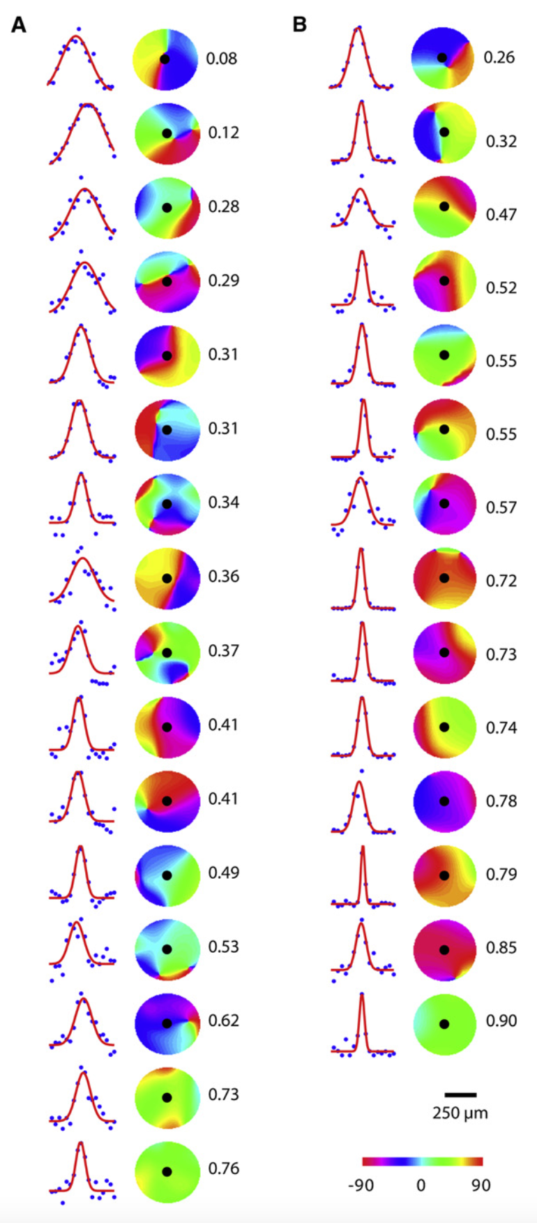
Figure 7: Measurements of the orientation tuning of neurons, at different positions in the visual cortex, according to Nauhaus et al. (2008) (Copyright Cell Press with permission). In this figure it can be seen how the orientation tuning changes from broad to sharp, and thus higher degree of orientation selectivity, with increasing distance from the pinwheels, consistent with the qualitative behaviour that would be obtained if the ratio $\kappa$, between the scale parameters in underlying affine Gaussian smoothing step in the idealized models of spatial and spatio-temporal receptive fields, would increase when moving away from the centers of the pinwheels on the cortical surface.

4 Implications for biological vision

In this section, we will compare the results of the above theoretical predictions with biological results concerning the orientation selectivity of visual neurons.

Nauhaus et al. (2008) have measured the orientation tuning of neurons at different positions in the primary visual cortex for monkey and cat. They found that the orientation tuning is broader near pinwheel centers and sharper in regions of homogeneous orientation preference. Figure 7 shows an overview of their results, where we can see how the degree of orientation selectivity changes rather continuously from broad to sharp with increasing distance from the pinwheel center (from top to bottom in the figure).

In view of our theoretical results in Section 3, concerning the orientation selectivity of receptive fields, where the spatial smoothing part is performed based on affine Gaussian kernels, this qualitative behaviour is consistent with what would be the result if the ratio $\kappa$ between the two scale parameters of the underlying affine Gaussian kernels would increase from a lower to a higher value, when moving away from the centers of the pinwheels on the cortical surface. Thus, the presented theory leads to a prediction about a variability in the eccentricity or elongation of the receptive fields in the primary visual cortex. In the case of pinwheel structures, the behaviour is specifically consistent with a variability in the eccentricity or elongation of the receptive fields from the centers of the pinwheels towards the periphery.

Furthermore, if we consider the theoretical prediction from (Lindeberg 2023b), that the shapes of the affine Gaussian derivative-based receptive fields ought to comprise a variability over a larger part of the affine group than mere rotations, to enable affine covariance and (partial) affine invariance at higher levels in the visual hierarchy. Then, if combined with the theoretical orientation selectivity analysis presented in the paper, those predictions are also consistent with the results by Nauhaus et al., with an additional explanatory power: If the theoretically motivated prediction would hold, then the underlying theoretical model may also enable a deeper interpretation of those biological results, in terms of underlying computational mechanisms in the visual receptive fields, to enable specific functional covariance and invariance properties at higher levels in the visual hierarchy.

It should be noted, however, that these predictions are not necessarily restricted to receptive fields according to the generalized affine Gaussian derivative model for receptive fields only. Qualitatively similar relationships between the orientation selectivity and the elongation of the receptive fields, can also be derived for other receptive field models, see Appendix A.1 for a qualitative Fourier analysis of qualitative orientation selectivity analysis of frequency-selective filters and Appendix A.2 for a more detailed study of the orientation selectivity for idealized receptive fields according to a purely spatial affine Gabor model.

A highly interesting quantitative measurement to perform, in view of these theoretical results, would hence be to fit parameterized models of the orientation selectivity, according to the summary in Table 1, to orientation tuning curves of the form recorded by Nauhaus et al. (2008), to get estimates of the distribution of the parameter $\kappa$ over a sufficiently large population of visual neurons, under the assumption that the spatial components of the biological receptive fields can be well modelled by affine Gaussian derivatives, as well as possibly extending such a model fitting to also comprise comparisons with the orientation selectivity curves obtained from the affine Gabor model of visual receptive fields (although those results are, so far, based on a purely spatial analysis of the receptive fields only).

In (Lindeberg 2023b), a theoretical treatment is given concerning covariance properties of visual receptive fields under natural image transformations, specifically geometric image transformations in terms of spatial scaling transformations, spatial affine transformations, Galilean transformations and temporal scaling transformations. According to that theory of spatial and spatio-temporal receptive fields, in terms of generalized Gaussian derivative based receptive fields, the covariance properties of the receptive fields mean that the shapes of the receptive field families should span the degrees of freedom generated by the geometric image transformations. With regard to spatial affine transformations, which beyond spatial scaling transformations do also comprise spatial rotations and non-uniform scaling transformation with different amount of scaling in two orthogonal spatial directions, this theory implies that affine Gaussian kernels ought to be present in the receptive field families corresponding to different values of the ratio $\kappa$ between the spatial scale parameters, in order to support affine covariance. In (Lindeberg 2023b Section 3.2) suggestions to new biological measurements were further proposed to support (or reject) those hypotheses.

If we would assume that it would be unlikely for the receptive fields to have as strong variability in their orientational selectivity properties as function of the positions of the neurons in relation to the pinwheel structure as reported in this study, without also having a strong variability in their eccentricity, then by combining the theoretical analysis in this article with the biological results by Nauhaus et al. (2008), that would serve as possible indirect support for the hypothesis concerning an expansion of receptive field shapes over variations in the ratio between the two scale parameters of spatially anisotropic receptive fields. If we would assume that the biological receptive fields can be well modelled by the generalized Gaussian derivative model based on affine Gaussian receptive fields, then the biological results by Nauhaus et al. (2008) are fully consistent with the prediction of such an explicit expansion over shapes of the visual receptive fields, based on the orientation selectivity of visual receptive fields, whose spatial smoothing component can be well modelled by affine Gaussian kernels.

Based on these results we propose that, beyond an expansion over rotations, as is performed in current models of the pinwheel structure of visual receptive fields (Bonhoeffer and Grinvald 1991; Blasdel 1992; Swindale 1996; Petitot 2003; Baspinar et al. 2018; Liu and Robinson 2022), also an explicit expansion over the eccentricity $\epsilon$ of the receptive fields (the inverse of the parameter $\kappa$) should be included, when modelling the pinwheel structure in the visual cortex.

Possible ways, by which an explicit dependency on the eccentricity of the receptive fields could be incorporated into the modelling of pinwheel structures, will be outlined in more detail in the following treatment regarding more specific biological hypotheses.

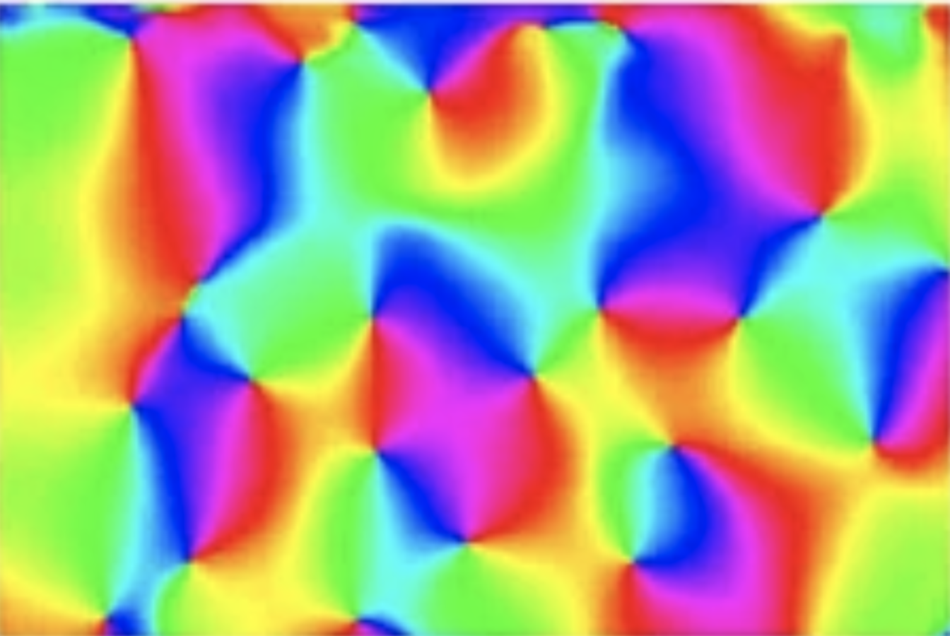
Figure 8: Orientation map in the primary visual cortex of cat, as recorded by Koch et al. (2016) (OpenAccess), with the orientation preference of the receptive fields encoded in terms of colours, and demonstrating that the visual cortex performs an explicit expansion of the receptive field shapes over spatial image orientations. A working hypothesis in the paper concerns to investigate whether the primary visual cortex could additionally perform an expansion over the eccentricity or the elongation of the spatial components of the receptive fields. One possible way of performing such an additional expansion, is over the spatial covariance matrices $\Sigma$ of the affine Gaussian derivative kernels according (1), and is illustrated in Figure 9, although that illustration would additionally need to be complemented by an identification of opposite image orientations, as, for example, can be achieved by a mapping to the double angle $\varphi\mapsto 2\varphi$, as well as a possible adjustment of the second degree of freedom, in how the variability of the two scale parameters in the affine Gaussian derivative model, beyond a variability over their ratio, varies from the center to the periphery in that illustration.

First-order affine Gaussian derivative kernels

Figure 9: Distribution of first-order affine Gaussian derivative kernels of the form (1), with a more explicit expression in Equation (7), for different spatial covariance matrices $\Sigma$, with their elements parameterized according to (4)–(6), with the larger spatial scale parameter $\sigma_{2}$ in this illustration held constant while the smaller scale parameter $\sigma_{1}$ varying as $\sigma_{1}=\sigma_{2}/\kappa$, according to a distribution on a hemisphere. The spatial directional derivatives, in turn, defined according to $\partial_{\varphi}=\cos\varphi\,\partial_{x_{1}}+\sin\varphi\,\partial_{x_{2}}$. The possible additional variability of the scale parameters, beyond their ratio $\kappa$, is, however, not explicitly addressed in this paper. From a biological viewpoint, one could, indeed, possibly think that it might be easier to keep the smaller scale parameter $\sigma_{2}$ constant and let the larger scale parameter $\sigma_{1}$ increase towards the periphery, since a higher degree of orientation selectivity can then be achieved by just integrating over successively larger support regions in the image space. The important aspect of this illustration is rather that the eccentricity $\kappa$ increases from the most isotropic image position towards the periphery. With regard to the possible connection to the pinwheel structure in the primary visual cortex, the center in this figure would correspond to the center of the pinwheel, whereas the periphery would correspond to the boundaries of the part of the visual cortex that is closest to the center of one particular pinwheel. (Reprinted from Lindeberg (2023b) (OpenAccess).)

4.1 Explicit testable hypotheses for biological experiments

Based on the above theoretical analysis with its associated theoretical predictions, we propose that it would be highly interesting to perform experimental characterization and analysis based on joint estimation of (i) orientational selectivity, (ii) receptive field eccentricity, (iii) orientational homogeneity and (iv) location of the neuron in the visual cortex in relation to the pinwheel structure, in the primary visual cortex of animals with clear pinwheel structures, to determine if there is a variability in the eccentricity or elongation of the receptive fields, and specifically if the degree of elongation increases with the distance from the centres of the pinwheels towards periphery, as arising as one possible interpretation of combining the theoretical results about orientation selectivity of affine Gaussian receptive fields in this article with the biological results by Nauhaus et al. (2008).

If additionally, reconstructions of the receptive field shapes could be performed for the receptive fields probed during such a systematic investigation of the difference in response characteristics with the distance from the pinwheel centers, and if the receptive fields could additionally be reasonably well modelled according to the generalized Gaussian model for receptive fields studied and used in this paper, it would be interesting to investigate of the shapes of the affine Gaussian components of these receptive fields would span a larger part of the affine group, than the span over mere image orientations, as already established in the orientation maps of the visual cortex, as characterized by Bonhoeffer and Grinvald 1991, Blasdel 1992 and others, see Figure 9 for an illustration.

If we would lay out the shapes of affine Gaussian receptive fields according to the shapes of their underlying spatial covariance matrices $\Sigma$, we would for a fixed value of their size (the spatial scale parameter) obtain a distribution of the form shown in Figure 9. That directional distribution is, however, in a certain aspect redundant, since opposite orientations on the unit circle are represented by two explicit copies, where the corresponding receptive fields are either equal, for receptive fields corresponding to spatial directional derivatives of even order, or of opposite sign for derivatives of even order. Could it be established that the receptive fields shapes, if expanded over a variability over eccentricity or elongation, for animals that have a clear pinwheel structure, have a spatial distribution that can somehow be related to such an idealized distribution, if we collapse opposite image orientations to the same image orientation, by e.g. a double-angle mapping $\varphi\mapsto 2\varphi$?

Notably the variability of the spatial covariance matrices in the affine Gaussian derivative model comprises a variability over two spatial scale parameters $\sigma_{1}$ and $\sigma_{2}$, while the theoretical analysis of the orientation selectivity properties studied in this article has mainly concerned their ratio $\kappa=\sigma_{2}/\sigma_{1}$. Hence, the illustration in Figure 9 should not be taken as a literal prediction, even if reduced by a double-angle representation. In Figure 9, the larger scale parameter $\sigma_{2}$ is held constant, for convenience of graphical illustration, as obtained by mapping the uniformly sized receptive fields from a uniform distribution on the hemisphere. More generally, one could also conceive other distributions as possible, such as, for example, instead keeping the smaller eigenvalue $\sigma_{1}$ constant from the center towards the periphery.

To conclude, we propose to state the following testable hypotheses for biological experiments:

Hypothesis 1 (Variability in eccentricity) Let $\sigma_{\varphi}$ and $\sigma_{\bot\varphi}$ be characteristic lengths in the preferred direction of an orientation selective simple cell in the primary visual cortex. Then, over a population of such simple cells, there is a substantial variability in their eccentricity ratio $\epsilon=\sigma_{\varphi}/\sigma_{\bot\varphi}$.

Hypothesis 2 (Variability in eccentricity coupled to orientational homogeneity) Assuming that Hypothesis 1 holds, let $\epsilon$ denote the eccentricity of a simple cell in the primary visual cortex, and let $H$ be a measure of the homogeneity in the orientation preference of its surrounding neurons. Then, over a population of simple cells. there is a systematic connection between $\epsilon$ and $H$.

Hypothesis 3 (Variability in eccentricity coupled to the pinwheel structure) Assuming that Hypothesis 1 holds, let $\epsilon$ denote the eccentricity of a simple cell in the primary visual cortex. Then, over a population of simple cells, there is a systematic connection between $\epsilon$ and the distance from the nearest pinwheel center.

If Hypothesis 3 would hold, then we could also sharpen this hypothesis further as:

Hypothesis 4 (Increase in elongation with increasing distance from the centers of the pinwheels) Assuming that Hypothesis 3 holds, let $\epsilon$ denote the eccentricity measure of a simple cell in the primary visual cortex defined such that this $\epsilon=1$ if the characteristic lengths of the spatial receptive fields are equal, and tending towards zero as the characteristic lengths differ more and more. Then, over a population of simple cells, the eccentricity measure decreases from the center of the pinwheel towards the periphery.

Note that the latter explicit hypotheses have been expressed on a general form, of not explicitly assuming that the biological receptive fields can be well modelled according to the generalized Gaussian derivative model for receptive fields. The essential part of the definition is only that it should be possible to define estimates of characteristic lengths $\sigma_{\varphi}$ and $\sigma_{\bot\varphi}$, so as to be able to define a measure of the eccentricity $\epsilon$.

If either Hypothesis 2 or Hypotesis 3 would hold, then we could also explicitly state the following hypothesis:

Hypothesis 5 (Pinwheel structure more structured than a mere expansion over spatial orientations) The pinwheel structure comprises an, at least, two-dimensional variability of receptive field shapes, beyond an expansion over spatial orientations, also an expansion over the eccentricity of the receptive fields in the primary visual cortex.

For simplicity, we have above expressed these hypotheses for the case of simple cells, for which it is easiest to define the measures $\sigma_{\varphi}$ and $\sigma_{\bot\varphi}$ of the characteristic lengths, because of the linearity of the receptive fields. Provided that corresponding measures of characteristic lengths could also be in a sufficiently well-established way be defined also for non-linear complex cells, corresponding explicit hypotheses could also be formulated for complex cells.

It should finally be stressed that, we have in this treatment not considered the binocular aspects of the pinwheel structure. In Hypothesis 5, the variability of the pinwheel structure over contributions from the left and the right eyes should therefore not be counted as a property to contribute to the terminology “more structured”.

4.2 Quantitative measurements for detailed characterization

To further characterize possible relationships between the orientational selectivity, receptive field eccentricity, orientational homogeneity, and the location of the neuron in relation to the pinwheel structure in the primary visual cortex, we would also propose to characterize the possible relationships between these entities in terms of:

Quantitative measurement 1: (Relationship between orientational selectivity and receptive field eccentricity) Graph or scatter diagram showing how a quantitative measure of orientational selectivity is related to a quantitative measure of receptive field eccentricity, accumulated over a sufficiently large population of neurons.

Quantitative measurement 2: (Relationship between orientational homogeneity and receptive field eccentricity) Graph or scatter diagram showing how a quantitative measure of orientational homogeneity is related to a quantitative measure receptive field eccentricity, accumulated over a sufficiently large population of neurons.

Quantitative measurement 3: (Relationship between receptive field eccentricity and the pinwheel structure) Graph or scatter diagram showing how a quantitative measure of receptive field eccentricity depends on the distance to the nearest pinwheel center, accumulated over a sufficiently large population of neurons.

Quantitative measurement 4: (Relationship between receptive field eccentricity and the pinwheel structure) Two-dimensional map showing how a quantitative measure of receptive field eccentricity relates to a two-dimensional map of the orientation preference over the same region in the primary visual cortex, with the center of the pinwheel structure explicitly marked, again accumulated over a sufficiently large population of neurons.

If the above theoretically motivated biological hypotheses can be investigated experimentally, and if the above quantitative measurements of receptive field characteristics could be performed, it could be judged if the prediction from the presented theoretical analysis about a systematic variability in receptive field eccentricity, with a possible relationship to the pinwheel structure, could be either experimentally supported or rejected. In a corresponding manner, such a judgement could also answer if the receptive fields in the primary visual cortex could be regarded as spanning a larger part of the affine group, than an expansion over mere rotations.

5 Relations to other possible receptive field models

In the treatment above, we have performed the analysis of properties of receptive fields in the primary visual cortex based on the generalized Gaussian derivative model for receptive fields. Main motivations for this choice are that:

• The idealized models of visual receptive fields can be derived from first principles in a theoretically well-founded manner, from the combination of a set of assumptions (axioms) that reflect structural properties of the world with a set of assumptions to guarantee internal consistency between image representations over multiple spatial and temporal scales,

• The idealized receptive field models arising from this theory show very good qualitative similarity to biological receptive fields in the retina, the lateral geniculate nucleus (LGN) and the primary visual cortex (V1),

• The idealized receptive field models according to this theory comprises theoretically well-founded models of both (i) purely spatial receptive fields, (ii) space-time separable spatio-temporal receptive fields and (iii) velocity-adapted spatio-temporal receptive fields.

• The resulting theory for models of visual receptive fields is intimately connected to the influence of natural geometric image transformations:

  • Spatial scaling transformations caused by objects in the world being of different physical size, or being at different distances to the observer.

  • Spatial affine transformations, that to first order of approximation approximate the non-linear perspective mapping from the tangent planes of smooth surfaces in the world to the visual sensorium.

  • Galilean transformations, that to first order of approximation approximate the influence on visual stimuli of objects that move with different velocities relative to the viewing direction.

  • Temporal scaling transformations, that capture the effects of spatio-temporal events occurring faster or slower.

  In this respect, the idealized receptive field models in the theory have the ability to handle the influence of natural image transformation on visual stimuli, to enable the computation of covariant or invariant representations with respect to these image transformations at higher levels in the visual hierarchy (Lindeberg 2023b).

• The receptive field model is biologically plausible in the sense that the output from the receptive fields operating on image data can be computed from a combination of (i) spatial diffusion processes that smooth the data over image space, (ii) computation of spatial derivative approximations from differences in relation to the nearest neighbours and (iii) temporal integration processes in terms of first-order temporal integrators, to compute temporal averages over time, complemented with (iv) linear combinations of image representations at multiple temporal scales, to compute approximations of temporal derivatives. Thus, the results of applying these idealized receptive field models to either a static image or a stream of video data can be computed with computational mechanisms that should be available to a network of biological neurons.

In these respects, the idealized models for visual receptive fields, that the theoretical analysis in this paper is based upon, should be regarded as both theoretically well-founded and biologically plausible.

The overall results from the analysis in this paper, that the orientation selectivity properties of the visual neurons should become more narrow for elongated receptive fields are, however, not unique to the generalized Gaussian derivative model for visual receptive fields. Nor will the biological predictions obtained by combining this theoretical result with the results by Nauhaus et al. (2008), that

• the receptive fields in the primary visual cortex should span a variability in the eccentricity or elongation,

• with respect to the ability of receptive fields to support covariance under spatial affine transformations, the shapes of visual receptive should span a larger part of the affine group than the subgroup of mere spatial rotations, to also span a variability over what corresponds to a variability over the ratio between the singular values of 2-D affine transformation matrices, and

• the pinwheel structure in the visual cortex should, in addition to an explicit expansion over spatial image orientations also comprise an expansion over the eccentricity of the receptive fields,

be restricted to an assumption that the biological receptive fields should necessarily be required to be well modelled by idealized receptive fields according to the generalized Gaussian derivative model for visual receptive fields.

In Appendix A.1, a qualitative argument is given of how a qualitative orientation selectivity analysis can be performed based on a qualitative Fourier analysis. If a particular model of an approximately rotationally symmetric spatial window function is fed into that model, and then combined with stretching in a certain image orientation, it should also be possible to derive a corresponding qualitative relationship that an increased degree of elongation of a receptive field should lead to a more narrow orientation selectivity.

In Appendix A.2, a more detailed quantitative orientation selectivity analysis is given for a purely spatial affine Gabor model of simple cells. First of all, the affine Gabor model is conceptually different from the affine Gaussian derivative model, in that it comprises one more degree of freedom, concerning variabilities in the angular frequency of the sine and cosine wave parts of the Gabor pair. For this affine Gabor model, a qualitatively similar result to the analysis of affine Gaussian derivative based receptive fields is, however, obtained, in that the orientation selectivity becomes more narrow, as the scale parameter ratio $\kappa$ increases.

The orientation selectivity of receptive fields of the affine Gabor model is, however, also strongly dependent on one more degree of freedom in the parameter space, corresponding to the product of the remaining spatial scale parameter $\sigma_{1}$ and the angular frequency $\nu$ in the Gabor model. Hence, if we would assume that a population of receptive fields would be generated from the full variability of the affine Gabor model, we would not, from a variability in the orientation selectivity of the receptive fields only, be able to logically infer that the receptive fields would be likely to span a variability over the elongation of the receptive fields. An increase in the orientation selectivity of the receptive fields could also be obtained from increasing the size of the receptive fields, while keeping the angular frequency constant. One could, however, then, on the other hand, also ask how biologically plausible such a variability would be, since the receptive fields would then look more and more like successively larger sine wave patches.

In Appendix A.3, a detailed analysis is given of the affine transformation property of a generalized purely spatial affine Gabor model of simple cells. It is shown that, if we allow for the angular frequency vector $\omega$ in an affine Gabor model of the form

$$G(x;\;\Sigma,\omega)=g(x;\;\Sigma,\omega)\,e^{i\omega^{T}x},$$ (90)

to be not necessarily required to be parallel with one of the eigendirections of the spatial covariance matrix $\Sigma$, then generalized affine Gabor representations computed by convolutions with this family of generalized affine Gabor functions are affine covariant.

If such a full generalization is, on the other hand, not performed, and angular frequency vector is required to be parallel with one of the eigendirections of the spatial covariance matrix $\Sigma$, then the resulting spatial receptive fields instead span the variabilities under (i) uniform spatial scaling transformations, (ii) spatial rotations and (iii) non-uniform spatial stretching transformations in the direction parallel with the angular frequency vector $\omega$.

With respect to the topic of a possible coupling between between a variability in the orientation selectivity of visual receptive fields, and whether the population of receptive fields could span a variability the degree of elongation of the receptive fields, the theoretical results in Appendix A.2 and Appendix A.3 do partially support such a connection. The connection is, however, weaker than for the previously treated affine Gaussian derivative model for visual receptive fields, in that the receptive fields according to the affine Gabor model do also comprise one more degree of freedom, by which a variability in the product of the scale parameter $\sigma_{1}$ and angular frequency $\nu$, would also lead to a variability in the orientation selectivity of the receptive fields.

In view of these results, it seems possible that connections between orientation selectivity analysis for biological vision in Section 4 could apply also for other classes of visual receptive fields than those studied specifically in Section 3 or Appendix A.2. Compared to the above qualitative analysis, based on the treatment in Appendix A.1, or the treatment of the spatial affine Gabor model in Appendix A.2 and Appendix A.3, the treatment in Section 3 does, however, provide added value in that it also performs a detailed analysis of genuine spatio-temporal receptive field models, and explicitly shows that the results obtained from a purely spatial domain do, in most of the cases, also generalize to joint spatio-temporal receptive field models.

A fundamental reason why we regard explicit incorporation of the dependency on the temporal dimension as essential in the theoretical modelling of neural responses in this context is that, a priori, it is highly probable that a particular visual neuron that is probed during a neurophysiological experiment will be sensitive to variabilities in the visual stimuli over time. If the theoretically derived model, on the other hand, has only been derived from a context where temporal dependencies are not explicitly modelled, then that would leave a much larger explanatory gap between the model and the neurophysiological reality, than if the model already from the beginning has been derived from a genuine spatio-temporal context.

In particular, with respect to one of our goals with this paper, of aiming at providing a theoretical foundation to make it possible to perform quantitative comparisons between the orientation selectivity curves of our idealized models of visual receptive fields with the orientation selectivity curves of actual visual neurons in the pinwheel structure in the primary visual cortex, we want to ensure that the theoretically derived models are consistent with the behaviour of genuine spatio-temporal receptive fields, that explicitly depend on variabilities along the temporal dimension.

According to our view, the influence of the temporal dimension on visual perception may not always be given as detailed investigation as it may warrant. For a detailed treatment of computational mechanisms to handle temporal data, including relations to temporal scales in visual and auditory receptive fields, as well as more generally to temporal multi-scale phenomena and mechanisms in neuroscience, see (Lindeberg 2023a.)

6 Summary and discussion

We have presented an in-depth theoretical analysis of the orientation selectivity for the spatial and spatio-temporal receptive fields according to the generalized Gaussian derivative model for visual receptive fields, summarized in Sections 2.1 and 2.3. This model for visual receptive fields has been previously derived in an axiomatic manner, from symmetry properties of the environment, in combination with requirements of internal consistency between image representations over multiple spatial and temporal scales. This model has notably also been demonstrated to well capture the properties of biological simple cells in the primary visual cortex. Building upon that theory for linear receptive fields, we have also analysed the orientation selectivity for (some of them new) non-linear models of complex cells, summarized in Sections 2.2 and 2.4, based on energy models that combine the output from such models for simple cells for different orders of spatial differentiation.

Specifically, we have in Section 3 analyzed how the orientation selectivity depends on a scale parameter ratio $\kappa$, between the scale parameters in the image orientations perpendicular to vs. parallel with the preferred orientation of the receptive fields. Explicit expressions for the resulting orientation tuning curves have been derived, based on closed form theoretical analysis, and it has been shown that, for all these models of visual receptive fields, the degree of orientation selectivity becomes more narrow with increasing values of the scale parameter ratio $\kappa$.

By comparisons with previously established results by Nauhaus et al. (2008), we have in Section 4 demonstrated that the predictions from our theory are consistent with general behaviour of visual neurons in the primary visual cortex, in that the orientation tuning is broader near the pinwheels, while the orientation selectivity becomes sharper further away.

By combining these two results, if we, would take the liberty of assuming that it would be unlikely for the population of receptive fields to exhibit a strong variability in the orientational selectivity of the receptive fields, without also similarly exhibiting a coupled variability in the eccentricity or the the degree of elongation of the receptive fields, then we would have possible indirect support for a previously formulated biological hypothesis in (Lindeberg 2023b), stating that the family of receptive field shapes should span the degrees of freedom in the natural geometric image transformations. That way of assumption-based reasoning would then specifically imply indirect support for the hypothesis that the receptive field shapes should span a sufficiently wide range of ratios between the scale parameters in the directions perpendicular to vs. parallel with the preferred orientation of the receptive field, to support affine covariance of the family of visual receptive fields.

Without explicitly relying on expressing such an explicit assumption, regarding whether the visual receptive fields in the primary visual cortex could be well modelled by affine Gaussian derivative based receptive fields, we can, however, firmly state that the biological measurements performed by Nauhaus et al. (2008) are, in combination with the theoretical results derived in Section 3 of this paper, consistent with the hypothesis that the receptive fields should span a variability in the eccentricity of the receptive fields. In this respect, the measurements that demonstrate a strong variability in orientation selectivity would specifically be consistent with the theoretically based hypothesis formulated in (Lindeberg 2023b), that the receptive fields in the primary visual cortex should span the variability of receptive field shapes under spatial affine transformations.

If we would apply a similar type of assumption-based logical reasoning to the pinwheel structure in the primary visual cortex, then such a reasoning, based on the results by Nauhaus et al. (2008), that the orientation selectivity appears to vary strongly from the centers of the pinwheels towards the periphery, would imply that the pinwheel structure in the visual cortex would, beyond an explicit expansion over image orientations, would also comprise an explicit expansion over the eccentricity or the degree of elongation of the receptive fields. Based on these predictions, we have specifically proposed that explicit dependencies on a variability in the eccentricity of the receptive fields should be included, when modelling the pinwheel structures in the primary visual cortex.

Strictly, and formally, the results from such logical inference could, however, only be regarded as theoretical predictions, to generate explicit hypothesis concerning the distribution of receptive field characteristics in these respects. To raise the question of determining if these theoretical predictions would hold in reality, we have in Section 4.1 formulated a set of testable explicit biological hypotheses, that could be either verified or rejected in neurophysiological experiments, concerning possible variabilities in the eccentricity of the receptive fields in the primary visual cortex of higher mammals, as well as hypotheses about possible connections between such variabilities in eccentricity or elongation and other receptive field characteristics, in particular in relation to the pinwheel structure in the primary visual cortex of higher mammals. We have also in Section 4.2 formulated a set of quantitative measurements that could be made, to characterize how a possible variability in the eccentricity of the receptive field could be related to other receptive field characteristics, including the pinwheel structure in the visual cortex.

To compare the theoretical predictions obtained based on the affine Gaussian derivative model for visual receptive fields, to what would be obtained from basing the theoretical analysis on other types of receptive field models, we have furthermore in Section 5 and Appendix A.2 presented a detailed orientation selectivity analysis for an an affine Gabor model of visual receptive fields. The results obtained from the affine Gabor model are consistent with the results obtained from the affine Gaussian derivative model, in the sense that the orientation selectivity becomes more narrow, as we widen the receptive fields in the direction perpendicular to preferred orientation of the receptive fields.

The results from the affine Gabor model do, on the other hand, also differ from the results obtained from the affine Gaussian derivative model, in the respect that the parameter space of the affine Gabor model comprises one more degree of freedom, compared to the parameter space of the affine Gaussian derivative model. Specifically, a variability along that additional degree of freedom does, as described in more detail in Appendix A.2, also strongly affect the orientation selectivity of the receptive fields according to the affine Gabor model. The predictions obtained from the affine Gaussian derivative model are in this respect more specific, regarding connections between the orientation selectivity and the elongation of the receptive fields. This points to a both a qualitative similarity and a qualitative difference between the affine Gaussian derivative model and the affine Gabor model.

We have also in Appendix A.3 shown that a generalized version of the affine Gabor model also supports affine covariance, as the affine Gaussian derivative model does.

Concerning extensions of the approach, we have in the present treatment regarding receptive fields according to the generalized Gaussian derivative model for visual receptive fields, limited ourselves to receptive fields corresponding to only first- and second-order derivatives over the spatial domain. Modelling results by Young (1987) have, however, demonstrated that receptive fields up to fourth order of spatial differentiation may be present in the primary visual cortex. It is straightforward to extend our analysis to third- and fourth-order directional derivatives, which would then give other closed-form expressions for the orientation selectivity of the receptive fields (and more narrow than the orientation selectivity for first- and second-order derivatives). Models of complex cells involving third- and fourth-order spatial derivatives could also be formulated and be theoretically analyzed, although experimental support for such extended models of complex cells may currently not be available.

A more conceptual way of extending the modelling work would also be to incorporate a complementary spatial smoothing step in model of complex cells, as used in (Lindeberg 2020 Section 5). In the models for complex cells used in the theoretical analysis in this paper, the responses of first- and second-order spatial derivative based receptive fields have been throughout combined in a pointwise manner, over both space and time. A more general approach would, however, be to perform weighted integration of such pointwise contributions over a wider support region over space and time, with the size over the spatial image domain and the duration over the temporal domain proportional to the local spatial and temporal scales at which the spatial and temporal derivatives are computed. In the present treatment, we have, however, not extended the complex cell models in that way, although it could be well motivated, mainly to simplify the treatment, and to limit the complexity of the theoretical analysis. If the orientation selectivity curves obtained from theoretical analysis are to be fitted to data from actual neurophysiological measurements, it does, however, seem advisable to complement the models for complex cells by explicit spatial integration, as done in Equation (46) in (Lindeberg 2020).

Concerning the spatio-temporal models of the receptive fields, we have also limited ourselves to performing a non-causal temporal analysis, where the temporal smoothing kernels are 1-D Gaussian kernels. To perform a corresponding time-causal temporal analysis, based on using the time-causal limit kernel (15) for temporal smoothing, one can perform a Fourier analysis to determine how the probing sine wave will be affected, using the closed-form expression for the Fourier transform of the time-causal limit kernel, in a similar way as in the temporal scale selection analysis in (Lindeberg 2017 Section 5.2).

Concerning the way that the orientation selectivity curves are defined, we have in the above theoretical analysis for the affine Gaussian derivative model throughout in Section 3 assumed that the wavelength $\hat{\omega}$ (and for the spatio-temporal analysis also the image velocity $\hat{u}$) of the probing sine wave is optimized for each image orientation separately. Another possibility is to instead assume that the wavelength is only optimized for the preferred orientation of the receptive field only, and then held constant for all the other inclination angles $\theta$. Changing the probing method in such a way would the change the shapes of the orientation selectivity curves, but could be easily performed, based on the principles for theoretical analysis outlined in the above treatment.

One could possibly also consider extending the analysis to different values of the scale normalization powers $\gamma$ and $\Gamma$, than using the maximally scale invariant choices $\gamma=1$ and $\Gamma=0$ used for simplicity in this treatment. Then, however, some type of post-normalization may, however, also be necessary, to make it possible to appropriately compare receptive field responses between multiple spatial and temporal scales, which otherwise are perfectly comparable when using $\gamma=1$ and $\Gamma=0$.

Concerning possible limitations of the approach, it should be emphasized that the models for visual receptive fields in the generalized Gaussian derivative model are highly idealized. They have been derived from mathematical analysis based on idealized theoretical assumptions, regarding symmetry properties of the environment, while have not been quantitatively adjusted to the receptive field shapes of actual biological neurons. Hence, the results from the presented theoretical analysis should be interpreted as such, as the results of a maximally idealized model, and not with specific aims of providing a numerically accurate representation of actual biological neurons. The receptive field models also constitute pure feed-forward models with no feed-back mechanisms, which are otherwise known to be important in biological vision. In view of such a background, it is, however, highly interesting to see how well the derived orientation selectivity curves in Figures 2, 4 and 5 reflect the qualitative shapes of the biologically established orientation selectivity curves in Figure 7.

It is also known that the distinction between simple and complex cells may not be as distinct as proposed in the initial work by Hubel and Wiesel, where there could instead be a scale of gradual transitions between simple and complex cells. Considering that the forms of the derived orientation selectivity are often similar for our models of simple and complex cells (as summarized in Table 1), one may speculate that the presented results could be relevant with respect to such a wider contextual background.

It may also be worth stating that we do not in any way exclude the possibility of deriving corresponding prediction results for other possible models of receptive fields, or for models of neural mechanisms that lead to the formation of visual receptive fields. A motivation for in this paper restricting the analysis in this paper to the idealized receptive fields according to the generalized Gaussian derivative model and to the idealized receptive fields according to the Gabor model, is that these models may be regarded the most commonly used and well-established idealized functional models for linear receptive fields in the primary visual cortex. These receptive field models do specifically reasonably well reproduce the qualitative shape of many receptive fields in the primary visual cortex, as have been established by neurophysiological measurements. The formulation of possible Gabor models for spatio-temporal receptive fields does, however, appear as a more open topic, why we restricted the analysis of the affine Gabor model to purely spatial receptive fields.

Concerning possible limitations in the hypothetical reasoning stages used for for possible logical inference and for formulating the explicit biological hypotheses above, based on explicitly stated assumptions regarding whether the biological receptive fields could be reasonably well modelled by affine Gaussian derivative based receptive fields, to be able to draw possible further conclusions, the possible validity of those hypothetical logical reasoning stages could, however, break down, if there would be other external factors, no covered by the theoretical model, that could also strongly influence the orientation selectivity of the receptive fields. The possible applicability of the hypothetical logical reasoning stages above, does, thus, ultimately depend on possible agreement between the model and biological data, and can only be taken further by performing more detailed actual model fitting (not performed here, because of lack of access to the data by Nauhaus et al. (2008)) and/or performing complementary neurophysiological experiments, to ultimately judge if the theoretically based predictions, stated more explicitly in Section 4.1, would hold for actual biological neurons.

In summary, we have with the presented treatment demonstrated how the generalized Gaussian derivative model for visual receptive fields lends itself to closed form theoretical analysis, that can lead to well-defined predictions between the orientation selectivity and the anisotropy or elongation of receptive fields in the primary visual cortex, and in this way qualitatively very reasonable predictions regarding phenomena in biological vision. We have specifically used these results to express possible indirect support for a biological hypothesis concerning expansion of receptive field shapes in the primary visual cortex over the degrees of freedom in natural geometric image transformations, regarding an expansion over the spatial eccentricity (the inverse of the scale parameter ratio $\kappa$) of the receptive fields. Based on these results, we specifically propose to also include such an expansion over eccentricity in models of the pinwheel structure of the receptive fields in the visual cortex. More generally, to ultimately judge if these theoretically based predictions would hold in the primary visual cortex of higher mammals, we have formulated a set of explicit hypotheses and quantitative measurements in Sections 4.1 and 4.2, that could serve as a guide to future neurophysiological experiments.

Appendix A Appendix

A.1 Qualitative orientation selectivity analysis by qualitative Fourier analysis

As a complement to the detailed orientation selectivity analysis in Section 3, for the specific classes of receptive field models in Section 2, it is also possible to arrive at qualitatively similar relationships between the orientation selectivity and the eccentricity or elongation of the receptive fields, by using a qualitative Fourier analysis of the following form:

• Assume that we can consider a class of non-negative spatial window functions that are smooth, localized in their spatial support, and thus having a low-pass spectrum.

• If the window function is stretched in one orientation in image space, then that will lead to an inverse stretching of the Fourier spectrum in the same direction. If the original window function is circular over the spatial domain, then the stretched window function will become more elliptic. The Fourier spectrum of the stretched window function will also attain a more elliptic shape, while with an opposite effect in terms of the stretching.

• To construct a filter that is sensitive to a particular frequency, generate a sine wave with that frequency and multiply with the stretched spatial window function. The Fourier transform of that filter will thus be the convolution between the Fourier transform of the stretched filter and the Fourier transform of the sine wave. Since the Fourier transform of the sine wave consists of two oppositely located delta functions in the Fourier domain, the Fourier transform of the frequency selective filter will consist of two oppositely located lobes in the Fourier domain.

• To perform an orientation selectivity analysis of this frequency-selective filter, we should convolve any probing sine wave having a possibly different orientation in image space by the frequency-selective spatial filter. In the Fourier domain, this corresponds to multiplying the Fourier transform of the probing sine wave, that is two oppositely located delta functions in the Fourier domain, by the Fourier transform of the frequency-selective filter.

• That multiplication for different image orientations thus corresponds to studying the value of the Fourier transform of the frequency-selective filter on a circle in the Fourier domain.

• Computing the inverse of the two amplitude- and phase-modulated delta functions will give a sine wave of the same frequency and orientation as the input probe, while with a different amplitude that represents the orientation selectivity, when combined with variations of the orientations of probing sine waves over all orientations in the image plane.

Such an approach could also be applied by replacing the sine waves in the above analysis by signals with a narrow frequency range.

This qualitative analysis indicates that the type of analysis performed in Section 3 is not restricted to receptive fields according to the generalized Gaussian derivative model only, but also to a wider class of frequency-selective models of receptive fields. The analysis in Section 3 does, however, provide more added value compared to such a qualitative analysis, in that it (i) applies to both purely spatial, space-time-separable and velocity-adapted models of receptive fields, as well as (ii) to both models of simple and complex cells, (iii) additionally optimizes the response over the frequency of the probing sine wave for each image orientation of the probing sine wave, and (iv) the results are obtained as closed-form mathematical expression, parameterized by the parameter $\kappa$ that represents the inverse eccentricity $\epsilon$. Additionally, the underlying affine Gaussian derivative based receptive field models for the orientation selectivity analysis in Section 3 have been determined in a theoretically principled manner.

	$\sigma_{1}\nu=1/2$	$\sigma_{1}\nu=1$	$\sigma_{1}\nu=2$
$\kappa=1$
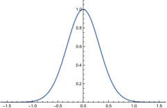
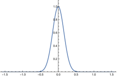
$\kappa=2$
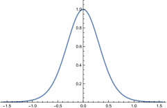
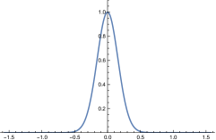
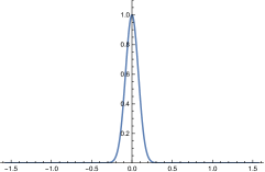
$\kappa=4$
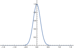
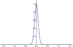
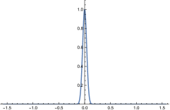
$\kappa=8$

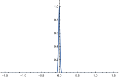
Figure 10: Graphs of the orientation selectivity of purely spatial models of a simple cell, using the even component of the affine Gabor model according to (91) and (92). Observe how the degree of orientation selectivity depends on the scale parameter ratio $\kappa$, in a qualitatively similar manner as for the affine Gaussian derivative model for purely spatial receptive fields. For the affine Gabor model, the degree of orientation selectivity does, however, also depend strongly on the product of the two remaining parameters $\sigma_{1}\,\nu$ in the model. (top row) Results for $\kappa=1$. (second row) Results for $\kappa=2$. (third row) Results for $\kappa=4$. (bottom row) Results for $\kappa=8$. (left column) Results for $\sigma_{1}\nu=1/2$. (middle column) Results for $\sigma_{1}\nu=1$. (right column) Results for $\sigma_{1}\nu=2$. (Horizontal axes: orientation $\theta\in[-\pi/2,\pi/2]$. Vertical axes: Amplitude of the receptive field response relative to the maximum response obtained for $\theta=0$.)

A.2 Orientation selectivity analysis for an affine Gabor model of simple cells

In this appendix, we will perform an orientation selectivity analysis, as analytically similar as possible, for idealized receptive fields according to an affine Gabor model for purely spatial receptive fields.

Given two spatial scale parameters $\sigma_{1}$ and $\sigma_{2}$ and an angular frequency $\nu$, consider an affine Gabor model with a pair of purely spatial receptive fields of the form

$$\begin{split}T_{even}(x_{1},x_{2};\;\sigma_{1},\sigma_{2},\nu)&=\frac{1}{2\pi\sigma_{1}\sigma_{2}}\,e^{-x_{1}^{2}/2\sigma_{1}^{2}-x^{2}/2\sigma_{2}^{2}}\cos(\nu x_{1}),\end{split}$$ (91)

$$\begin{split}T_{odd}(x_{1},x_{2};\;\sigma_{1},\sigma_{2},\nu)&=\frac{1}{2\pi\sigma_{1}\sigma_{2}}\,e^{-x_{1}^{2}/2\sigma_{1}^{2}-x^{2}/2\sigma_{2}^{2}}\sin(\nu x_{1}).\end{split}$$ (92)

Let us, in analogy with the treatment in Section 3.3, subject these receptive fields to test probes of the form (27)

$$f(x_{1},x_{2})=\sin\left(\omega\cos(\theta)\,x_{1}+\omega\sin(\theta)\,x_{2}+\beta\right).$$ (93)

for different inclination angles $\theta$. The responses of the even and odd components of the Gabor pair to such test functions are given by

$$\begin{split}L_{even}(x_{1},x_{2};\;\sigma_{1},\sigma_{2},\nu)=\end{split}$$

$$\begin{split}&=\int_{\xi_{1}=-\infty}^{\infty}\int_{\xi_{2}=-\infty}^{\infty}T_{even}(\xi_{1},\xi_{2};\;\sigma_{1},\sigma_{2},\nu)\end{split}$$

$$\begin{split}&\phantom{==\int_{\xi_{1}=-\infty}^{\infty}\int_{\xi_{2}=-\infty}^{\infty}}\times f(x_{1}-\xi_{1},x_{2}-\xi_{2})\,d\xi_{1}\xi_{2},\end{split}$$

$$\begin{split}L_{odd}(x_{1},x_{2};\;\sigma_{1},\sigma_{2},\nu)=\end{split}$$

$$\begin{split}&=\int_{\xi_{1}=-\infty}^{\infty}\int_{\xi_{2}=-\infty}^{\infty}T_{odd}(\xi_{1},\xi_{2};\;\sigma_{1},\sigma_{2},\nu)\end{split}$$

$$\begin{split}&\phantom{==\int_{\xi_{1}=-\infty}^{\infty}\int_{\xi_{2}=-\infty}^{\infty}}\times f(x_{1}-\xi_{1},x_{2}-\xi_{2})\,d\xi_{1}\xi_{2}.\end{split}$$ (94)

Solving these convolution integrals in Mathematica then gives

$$\begin{split}L_{even}(x_{1},x_{2};\;\sigma_{1},\sigma_{2},\nu)=\end{split}$$

$$\begin{split}&=\frac{1}{2}\left(e^{2\nu\omega\sigma_{1}^{2}\cos\theta}+1\right)\sin(\beta+\omega x\cos\theta+\omega y\sin\theta)\times\end{split}$$

$$\begin{split}&\phantom{=}\quad e^{\frac{1}{2}\left(-\nu^{2}\sigma_{1}^{2}-2\nu\omega\sigma_{1}^{2}\cos\theta-\omega^{2}\sigma_{1}^{2}\cos^{2}\theta-\omega^{2}\sigma_{2}^{2}\sin^{2}\theta\right)},\end{split}$$ (95)

$$\begin{split}L_{odd}(x_{1},x_{2};\;\sigma_{1},\sigma_{2},\nu)=\end{split}$$

$$\begin{split}&=-\frac{1}{2}\left(e^{2\nu\omega\sigma_{1}^{2}\cos\theta}-1\right)\cos(\beta+\omega x\cos\theta+\omega y\sin\theta)\times\end{split}$$

$$\begin{split}&\phantom{=}\quad e^{\frac{1}{2}\left(-\nu^{2}\sigma_{1}^{2}-2\nu\omega\sigma_{1}^{2}\cos\theta-\omega^{2}\sigma_{1}^{2}\cos^{2}\theta-\omega^{2}\sigma_{2}^{2}\sin^{2}\theta\right)}.\end{split}$$ (96)

Unfortunately, it is hard to analytically determine the angular frequency $\omega$ of the test function that gives the strongest amplitude for the Gabor response obtained with a given frequency $\nu$. Therefore, we will in the following simply set $\omega=\nu$, implying that this analysis for the Gabor model will not be methodologically identical to the previous analysis for the affine Gaussian derivative model, in the sense that we will not optimize the angular frequency $\omega$ of the test probe for each inclination angle $\theta$.

Letting additionally $\sigma_{2}=\kappa\,\sigma_{1}$ for $\kappa>1$, we obtain that the amplitudes of the two Gabor responses can be written:

$$\begin{split}A_{even}=\frac{1}{2}\left(e^{2\nu^{2}\sigma_{1}^{2}\cos\theta}+1\right)e^{-\nu^{2}\sigma_{1}^{2}\cos^{2}\left(\frac{\theta}{2}\right)(\kappa^{2}-1)(1-\cos\theta)},\end{split}$$ (97)

$$\begin{split}A_{odd}=\frac{1}{2}\left(e^{2\nu^{2}\sigma_{1}^{2}\cos\theta}-1\right)e^{-\nu^{2}\sigma_{1}^{2}\cos^{2}\left(\frac{\theta}{2}\right)(\kappa^{2}-1)(1-\cos\theta)},\end{split}$$ (98)

In contrast to the previous analysis for affine Gaussian derivative models of simple cells, where we determined the angular frequency of the probing sine wave, to maximize the response given a value of the spatial scale parameter, and in this way eliminated the dependency of the orientation selectivity on the size of the spatial scale parameter in the idealized receptive field model, and in this way reduced the explicit orientation dependency to only depend on the ratio $\kappa$ between the scale parameters, we cannot, however, here eliminate the remaining parameters of the idealized Gabor model from the orientation selectivity analysis.

The affine Gabor model comprises three internal parameters for the receptive fields (the spatial scale parameters $\sigma_{1}$ and $\sigma_{2}$, the angular frequency $\nu$ as well as the here not explicitly modelled orientation angle $\varphi$), while the purely spatial affine Gaussian derivative model comprises only three internal parameters (the spatial scale parameters $\sigma_{1}$ and $\sigma_{2}$ as well as the in Section 3 neither explicitly modelled orientation angle $\varphi$).

The affine Gabor model, thus, comprises one more parameter than the affine Gaussian derivative model. The dependency on the remaining degrees of freedom (beyond the orientation $\varphi$), due to variations in $\sigma_{1}$ and $\nu$, is, however, of a special form, in the respect that the dependency only depends on the product between $\sigma_{1}$ and $\nu$. Therefore, we will have to, beyond a variability with respect to the scale parameter ratio $\kappa$, also investigate the behaviour with respect to variations of the product of the angular frequency $\nu$ and the remaining spatial scale parameter $\sigma_{1}$.

Figure 10 shows orientation selectivity curves for the even component of the affine Gabor pair for different combinations of the scale parameter ratio $\kappa=1,2,4$ and $8$ and the product $\sigma_{1}\nu=1/2,1$ and $2$. As can be seen from these graphs, the orientation selectivity becomes more narrow with increasing values of the scale parameter ratio $\kappa$, as for the affine Gaussian derivative model. The orientation selectivity does, however, also become more narrow when the product $\sigma_{1}\,\nu$ increases.

Hence, from the conceptual background of whether one could possibly infer that the receptive fields ought to be more elongated, when the orientation selectivity becomes more narrow, one would not be able to make such a logical inference from a population of neurons according to the affine Gabor model, if the only a priori would be that the population would be generated from an expansion over all the four internal parameters $\sigma_{1}$, $\kappa$, $\nu$ and the orientation $\varphi$. If it, on the other hand, would be a priori known that the relationship between the angular frequency $\nu$ and the remaining spatial scale parameter $\sigma_{1}$ would be fixed to a fixed to their product being held constant, then one would, in principle, be able to make such a logical inference.

To save space, we do not show the graphs for the corresponding orientation selectivity curves for the odd component of the Gabor pair, nor for the idealized model of a complex cell, obtained by squaring the responses from the odd and even components and then adding them, and finally taking the square root of the result:

$$\begin{split}Q^{2}=L_{even}^{2}+L_{odd}^{2}\end{split}$$

$$\begin{split}=\frac{1}{4}e^{-\nu^{2}\sigma_{1}^{2}\left(\kappa^{2}\sin^{2}\theta+\cos^{2}\theta+2\cos\theta+1\right)}\times\end{split}$$

$$\begin{split}\phantom{=}\left(1+e^{4\nu^{2}\sigma_{1}^{2}\cos\theta}\right.\end{split}$$

$$\begin{split}\phantom{=}\left.\quad-2\,e^{2\nu^{2}\sigma_{1}^{2}\cos\theta}\cos(2(\beta+\nu x\cos\theta+\nu y\sin\theta))\right).\end{split}$$ (99)

The qualitative results, that receptive fields become more narrow as the scale parameter ratio $\kappa$ increases, or the product $\sigma_{1}\nu$ of the two remaining parameters increases, are, however, similar. So are the results that the orientation selectivity of the receptive fields, however, also depends strongly upon the product $\sigma_{1}\nu$.

We refrain from extending the analysis to possible spatio-temporal models, since it may not be fully clear how the spatio-temporal Gabor models should then be defined.

A.3 Affine transformation property for receptive fields according to a generalized affine Gabor model for simple cells

Given any positive definite spatial covariance matrix $\Sigma$ and any angular frequency vector $\omega=(\omega_{1},\omega_{2})^{T}$, consider a generalization of the affine Gabor model (91) to a vector-valued affine Gabor function of the form

$$G(x;\;\Sigma,\omega)=g(x;\;\Sigma,\omega)\,e^{i\omega^{T}x},$$ (100)

where $g(x;\;\Sigma,\omega)$ denotes a (here) two-dimensional Gaussian kernel

$$g(x;\;\Sigma)=\frac{1}{2\pi\sqrt{\det\Sigma}}\,e^{-x^{T}\Sigma^{-1}x/2}.$$ (101)

In the case when the angular frequency vector $\omega$ is parallel to one of the eigenvectors of the spatial covariance matrix $\Sigma$, this form of affine Gabor function spans a similar variability as the previously treated affine Gabor model in (91). To make it possible to define a representation that is closed under general affine transformations (affine covariance), we do, however, here, relax the assumption that the orientation of the angular frequency vector $\omega$ should be related to the dominant orientations defined by the eigendirections of the spatial covariance matrix $\Sigma$.

Let us now assume that we have two spatial images $f(x)$ and $f^{\prime}(x^{\prime})$ that are related according to a spatial affine transformation, such that

$$f^{\prime}(x^{\prime})=f(x)$$ (102)

for

$$x^{\prime}=A\,x.$$ (103)

Let us furthermore define affine Gabor representations over the two spatial domains according to

$$\begin{split}L(x;\,\Sigma,\omega)&=(G(\cdot;\;\Sigma,\omega)*f(\cdot))(x;\;\Sigma,\omega)\end{split}$$

$$\begin{split}&=\int_{\xi\in{\mathbb{R}}^{2}}G(\xi;\;\Sigma,\omega)\,f(x-\xi)\,d\xi,\end{split}$$ (104)

$$\begin{split}L^{\prime}(x^{\prime};\,\Sigma^{\prime},\omega^{\prime})&=(G(\cdot;\;\Sigma^{\prime},\omega^{\prime})*f^{\prime}(\cdot))(x^{\prime};\;\Sigma^{\prime},\omega^{\prime})\end{split}$$

$$\begin{split}&=\int_{\xi^{\prime}\in{\mathbb{R}}^{2}}G(\xi^{\prime};\;\Sigma^{\prime},\omega^{\prime})\,f(x^{\prime}-\xi^{\prime})\,d\xi^{\prime}.\end{split}$$ (105)

We would now like to investigate if the affine Gabor representations over the two domains could be related to each other. To express such a relation, we will perform the change of variables

$$\xi^{\prime}=A\,\xi,$$ (106)

which gives

$$d\xi^{\prime}=|\det A|\,d\xi,$$ (107)

in the convolution integrals.

Step I: Let us first consider how the Gaussian function $g^{\prime}(x^{\prime};\,\Sigma^{\prime})$ in the Gabor function $G(x^{\prime};\;\Sigma^{\prime},\omega^{\prime})$ transforms under the change of variables. If we, in analogy with the transformation property of the spatial covariance matrix in the affine Gaussian derivative model for visual receptive fields (Equation (28) in Lindeberg 2023b) assume that

$$\Sigma^{\prime}=A\,\Sigma\,A^{T},$$ (108)

which gives

$${\Sigma^{\prime}}^{-1}=A^{-T}\,\Sigma^{-1}\,A^{-1}$$ (109)

and

$$\det\Sigma^{\prime}=|\det A|^{2}\,\det\Sigma,$$ (110)

then we obtain

$$\begin{split}g(\xi^{\prime};\;\Sigma^{\prime})=\frac{1}{2\pi\sqrt{\det\Sigma^{\prime}}}\,e^{-{\xi^{\prime}}^{T}{\Sigma^{\prime}}^{-1}\xi^{\prime}/2}\end{split}$$

$$\begin{split}=\frac{1}{2\pi|\det A|\sqrt{\det\Sigma}}\,e^{-{A\xi}^{T}A^{-T}\,\Sigma^{-1}\,A^{-1}A\xi/2}\end{split}$$ (111)

$$\begin{split}=\frac{1}{|\det A|}\,\frac{1}{2\pi\sqrt{\det\Sigma}}\,e^{-\xi^{T}\,\Sigma^{-1}\xi/2}=\frac{1}{|\det A|}\,g(\xi;\;\Sigma).\end{split}$$ (112)

Step II: If we further set

$$\omega^{\prime}=A^{-T}\omega,$$ (113)

and combine with the transformation property (112) of the affine Gaussian kernel, then we have that the Gabor functions over the two domains are related according to

$$\begin{split}G(\xi^{\prime};\;\Sigma^{\prime},\omega^{\prime})=g(\xi^{\prime};\;\Sigma^{\prime})\,e^{i{\omega^{\prime}}^{T}\xi^{\prime}}=\frac{1}{|\det A|}\,g(\xi;\;\Sigma)\,e^{i(A^{-T}\omega)^{T}A\xi}\end{split}$$

$$\begin{split}=\frac{1}{|\det A|}\,g(\xi;\;\Sigma)\,e^{i\omega^{T}\xi}=\frac{1}{|\det A|}\,G(\xi;\;\Sigma,\omega).\end{split}$$ (114)

Step III: Applied to the convolution integrals (LABEL:eq-def-gabor-transf-conv-int1-proof) and (LABEL:eq-def-gabor-transf-conv-int2-proof), the transformation property (114) of the genuinely affine Gabor function (100) thus implies that

$$\begin{split}L^{\prime}(x^{\prime};\,\Sigma^{\prime},\omega^{\prime})=(G(\cdot;\;\Sigma^{\prime},\omega^{\prime})*f^{\prime}(\cdot))(x^{\prime};\;\Sigma^{\prime},\omega^{\prime})\end{split}$$

$$\begin{split}=\int_{\xi^{\prime}\in{\mathbb{R}}^{2}}G(\xi^{\prime};\;\Sigma^{\prime},\omega^{\prime})\,f(x^{\prime}-\xi^{\prime})\,d\xi^{\prime}.\end{split}$$

$$\begin{split}=\int_{\xi\in{\mathbb{R}}^{2}}\frac{1}{|\det A|}\,G(\xi;\;\Sigma,\omega)\,f(x-\xi)\,|\det A|\,d\xi,\end{split}$$

$$\begin{split}=(G(\cdot;\;\Sigma,\omega)*f(\cdot))(x;\;\Sigma,\omega)=L(x;\,\Sigma,\omega).\end{split}$$ (115)

Summary of main result: To conclude, we have shown that if two images $f(x)$ and $f^{\prime}(x^{\prime})$ are related according to an affine transformation

$$f^{\prime}(x^{\prime})=f(x)$$ (116)

where

$$x^{\prime}=A\,x,$$ (117)

then provided that affine Gabor representations are defined over the two spatial domains according to

$$\begin{split}L(x;\,\Sigma,\omega)&=(G(\cdot;\;\Sigma,\omega)*f(\cdot))(x;\;\Sigma,\omega),\end{split}$$ (118)

$$\begin{split}L^{\prime}(x^{\prime};\,\Sigma^{\prime},\omega^{\prime})&=(G(\cdot;\;\Sigma^{\prime},\omega^{\prime})*f^{\prime}(\cdot))(x^{\prime};\;\Sigma^{\prime},\omega^{\prime}),\end{split}$$ (119)

it then follows that these (genuinely) affine Gabor representations are equal under a similar spatial affine transformation

$$L^{\prime}(x^{\prime};\,\Sigma^{\prime},\omega^{\prime})=L(x;\,\Sigma,\omega),$$ (120)

provided that the values of the receptive field parameters $\Sigma$, $\Sigma^{\prime}$, $\omega$ and $\omega^{\prime}$ are appropriately matched according to

$$\begin{split}\Sigma^{\prime}=A\,\Sigma\,A^{T},\end{split}$$ (121)

$$\begin{split}\omega^{\prime}=A^{-T}\omega.\end{split}$$ (122)

This affine transformation property constitutes a genuine affine covariance property of the (here) generalized family of affine Gabor functions according to

$$G(x;\;\Sigma,\omega)=g(x;\;\Sigma,\omega)\,e^{i\omega^{T}x}.$$ (123)

In this context, it should, however, be noted that restricted affine Gabor model (91), where the angular frequency vector is restricted to be parallel with one of the eigendirections of the spatial covariance matrix $\Sigma$, cannot, however, be expected to be covariant over the complete group of spatial affine transformations. That restricted affine Gabor model will, however, be covariant under similarity transformations (uniform scaling transformations and spatial rotations) as well as to stretching transformations in the orientation of the angular frequency vector.

References

- Adelson and Bergen [1985] E. Adelson and J. Bergen. Spatiotemporal energy models for the perception of motion. Journal of Optical Society of America, A 2:284–299, 1985.
- Baspinar et al. [2018] E. Baspinar, G. Citti, and A. Sarti. A geometric model of multi-scale orientation preference maps via Gabor functions. Journal of Mathematical Imaging and Vision, 60:900–912, 2018.
- Berkes and Wiskott [2005] P. Berkes and L. Wiskott. Slow feature analysis yields a rich repertoire of complex cell properties. Journal of Vision, 5(6):579–602, 2005.
- Blasdel [1992] G. G. Blasdel. Orientation selectivity, preference and continuity in monkey striate cortex. Journal of Neuroscience, 12(8):3139–3161, 1992.
- Bonhoeffer and Grinvald [1991] T. Bonhoeffer and A. Grinvald. Iso-orientation domains in cat visual cortex are arranged in pinwheel-like patterns. Nature, 353:429–431, 1991.
- Bracewell [1999] R. N. Bracewell. The Fourier Transform and its Applications. McGraw-Hill, New York, 1999. 3rd edition.
- Carandini [2006] M. Carandini. What simple and complex cells compute. The Journal of Physiology, 577(2):463–466, 2006.
- Conway and Livingstone [2006] B. R. Conway and M. S. Livingstone. Spatial and temporal properties of cone signals in alert macaque primary visual cortex. Journal of Neuroscience, 26(42):10826–10846, 2006.
- De and Horwitz [2021] A. De and G. D. Horwitz. Spatial receptive field structure of double-opponent cells in macaque V1. Journal of Neurophysiology, 125(3):843–857, 2021.
- DeAngelis and Anzai [2004] G. C. DeAngelis and A. Anzai. A modern view of the classical receptive field: Linear and non-linear spatio-temporal processing by V1 neurons. In L. M. Chalupa and J. S. Werner, editors, The Visual Neurosciences, volume 1, pages 704–719. MIT Press, 2004.
- DeAngelis et al. [1995] G. C. DeAngelis, I. Ohzawa, and R. D. Freeman. Receptive field dynamics in the central visual pathways. Trends in Neuroscience, 18(10):451–457, 1995.
- Einhäuser et al. [2002] W. Einhäuser, C. Kayser, P. König, and K. P. Körding. Learning the invariance properties of complex cells from their responses to natural stimuli. European Journal of Neuroscience, 15(3):475–486, 2002.
- Emerson et al. [1987] R. C. Emerson, M. C. Citron, W. J. Vaughn, and S. A. Klein. Nonlinear directionally selective subunits in complex cells of cat striate cortex. Journal of Neurophysiology, 58(1):33–65, 1987.
- Georgeson et al. [2007] M. A. Georgeson, K. A. May, T. C. A. Freeman, and G. S. Hesse. From filters to features: Scale-space analysis of edge and blur coding in human vision. Journal of Vision, 7(13):7.1–21, 2007.
- Goris et al. [2015] R. L. T. Goris, E. P. Simoncelli, and J. A. Movshon. Origin and function of tuning diversity in Macaque visual cortex. Neuron, 88(4):819–831, 2015.
- Hansard and Horaud [2011] M. Hansard and R. Horaud. A differential model of the complex cell. Neural Computation, 23(9):2324–2357, 2011.
- Hansen and Neumann [2008] T. Hansen and H. Neumann. A recurrent model of contour integration in primary visual cortex. Journal of Vision, 8(8):8.1–25, 2008.
- Heeger [1992] D. J. Heeger. Normalization of cell responses in cat striate cortex. Visual Neuroscience, 9:181–197, 1992.
- Hesse and Georgeson [2005] G. S. Hesse and M. A. Georgeson. Edges and bars: where do people see features in 1-D images? Vision Research, 45(4):507–525, 2005.
- Hubel and Wiesel [1959] D. H. Hubel and T. N. Wiesel. Receptive fields of single neurones in the cat’s striate cortex. J Physiol, 147:226–238, 1959.
- Hubel and Wiesel [1962] D. H. Hubel and T. N. Wiesel. Receptive fields, binocular interaction and functional architecture in the cat’s visual cortex. J Physiol, 160:106–154, 1962.
- Hubel and Wiesel [2005] D. H. Hubel and T. N. Wiesel. Brain and Visual Perception: The Story of a 25-Year Collaboration. Oxford University Press, 2005.
- Johnson et al. [2008] E. N. Johnson, M. J. Hawken, and R. Shapley. The orientation selectivity of color-responsive neurons in Macaque V1. The Journal of Neuroscience, 28(32):8096–8106, 2008.
- Jones and Palmer [1987a] J. Jones and L. Palmer. The two-dimensional spatial structure of simple receptive fields in cat striate cortex. J. of Neurophysiology, 58:1187–1211, 1987a.
- Jones and Palmer [1987b] J. Jones and L. Palmer. An evaluation of the two-dimensional Gabor filter model of simple receptive fields in cat striate cortex. J. of Neurophysiology, 58:1233–1258, 1987b.
- Koch et al. [2016] E. Koch, J. Jin, J. M. Alonso, and Q. Zaidi. Functional implications of orientation maps in primary visual cortex. Nature Communications, 7(1):13529, 2016.
- Koenderink [1984] J. J. Koenderink. The structure of images. Biological Cybernetics, 50(5):363–370, 1984.
- Koenderink and van Doorn [1987] J. J. Koenderink and A. J. van Doorn. Representation of local geometry in the visual system. Biological Cybernetics, 55(6):367–375, 1987.
- Koenderink and van Doorn [1990] J. J. Koenderink and A. J. van Doorn. Receptive field families. Biological Cybernetics, 63:291–298, 1990.
- Koenderink and van Doorn [1992] J. J. Koenderink and A. J. van Doorn. Generic neighborhood operators. IEEE Transactions on Pattern Analysis and Machine Intelligence, 14(6):597–605, Jun. 1992.
- Kording et al. [2004] K. P. Kording, C. Kayser, W. Einhäuser, and P. Konig. How are complex cell properties adapted to the statistics of natural stimuli? Journal of Neurophysiology, 91(1):206–212, 2004.
- Lindeberg [1998] T. Lindeberg. Feature detection with automatic scale selection. International Journal of Computer Vision, 30(2):77–116, 1998.
- Lindeberg [2011] T. Lindeberg. Generalized Gaussian scale-space axiomatics comprising linear scale-space, affine scale-space and spatio-temporal scale-space. Journal of Mathematical Imaging and Vision, 40(1):36–81, 2011.
- Lindeberg [2013] T. Lindeberg. A computational theory of visual receptive fields. Biological Cybernetics, 107(6):589–635, 2013.
- Lindeberg [2016] T. Lindeberg. Time-causal and time-recursive spatio-temporal receptive fields. Journal of Mathematical Imaging and Vision, 55(1):50–88, 2016.
- Lindeberg [2017] T. Lindeberg. Temporal scale selection in time-causal scale space. Journal of Mathematical Imaging and Vision, 58(1):57–101, 2017.
- Lindeberg [2018] T. Lindeberg. Dense scale selection over space, time and space-time. SIAM Journal on Imaging Sciences, 11(1):407–441, 2018.
- Lindeberg [2020] T. Lindeberg. Provably scale-covariant continuous hierarchical networks based on scale-normalized differential expressions coupled in cascade. Journal of Mathematical Imaging and Vision, 62(1):120–148, 2020.
- Lindeberg [2021] T. Lindeberg. Normative theory of visual receptive fields. Heliyon, 7(1):e05897:1–20, 2021. doi: 10.1016/j.heliyon.2021.e05897.
- Lindeberg [2023a] T. Lindeberg. A time-causal and time-recursive scale-covariant scale-space representation of temporal signals and past time. Biological Cybernetics, 117(1–2):21–59, 2023a.
- Lindeberg [2023b] T. Lindeberg. Covariance properties under natural image transformations for the generalized Gaussian derivative model for visual receptive fields. Frontiers in Computational Neuroscience, 17:1189949:1–23, 2023b.
- Liu and Robinson [2022] X. Liu and P. A. Robinson. Analytic model for feature maps in the primary visual cortex. Frontiers in Computational Neuroscience, 16:2, 2022.
- Lowe [2000] D. G. Lowe. Towards a computational model for object recognition in IT cortex. In Biologically Motivated Computer Vision, volume 1811 of Springer LNCS, pages 20–31. Springer, 2000.
- Marcelja [1980] S. Marcelja. Mathematical description of the responses of simple cortical cells. Journal of Optical Society of America, 70(11):1297–1300, 1980.
- May and Georgeson [2007] K. A. May and M. A. Georgeson. Blurred edges look faint, and faint edges look sharp: The effect of a gradient threshold in a multi-scale edge coding model. Vision Research, 47(13):1705–1720, 2007.
- Merolla and Boahn [2004] P. Merolla and K. Boahn. A recurrent model of orientation maps with simple and complex cells. In Advances in Neural Information Processing Systems (NIPS 2004), pages 995–1002, 2004.
- Movshon et al. [1978] J. A. Movshon, E. D. Thompson, and D. J. Tolhurst. Receptive field organization of complex cells in the cat’s striate cortex. The Journal of Physiology, 283(1):79–99, 1978.
- Nauhaus et al. [2008] I. Nauhaus, A. Benucci, M. Carandini, and D. L. Ringach. Neuronal selectivity and local map structure in visual cortex. Neuron, 57(5):673–679, 2008.
- Pei et al. [2016] Z.-J. Pei, G.-X. Gao, B. Hao, Q.-L. Qiao, and H.-J. Ai. A cascade model of information processing and encoding for retinal prosthesis. Neural Regeneration Research, 11(4):646, 2016.
- Petitot [2003] J. Petitot. The neurogeometry of pinwheels as a sub-Riemannian contact structure. Journal of Physiology-Paris, 97(2–3):265–309, 2003.
- Porat and Zeevi [1988] M. Porat and Y. Y. Zeevi. The generalized Gabor scheme of image representation in biological and machine vision. IEEE Transactions on Pattern Analysis and Machine Intelligence, 10(4):452–468, 1988.
- Ringach [2002] D. L. Ringach. Spatial structure and symmetry of simple-cell receptive fields in macaque primary visual cortex. Journal of Neurophysiology, 88:455–463, 2002.
- Ringach [2004] D. L. Ringach. Mapping receptive fields in primary visual cortex. Journal of Physiology, 558(3):717–728, 2004.
- Ringach et al. [2002] D. L. Ringach, R. M. Shapley, and M. J. Hawken. Orientation selectivity in macaque V1: Diversity and laminar dependence. Journal of Neuroscience, 22(13):5639–5651, 2002.
- Rose and Blakemore [1974] D. Rose and C. Blakemore. An analysis of orientation selectivity in the cat’s visual cortex. Experimental Brain Research, 20:1–17, 1974.
- Rust et al. [2005] N. C. Rust, O. Schwartz, J. A. Movshon, and E. P. Simoncelli. Spatiotemporal elements of macaque V1 receptive fields. Neuron, 46(6):945–956, 2005.
- Sasaki et al. [2015] K. S. Sasaki, R. Kimura, T. Ninomiya, Y. Tabuchi, H. Tanaka, M. Fukui, Y. C. Asada, T. Arai, M. Inagaki, T. Nakazono, M. Baba, K. Daisuke, S. Nishimoto, T. M. Sanada, T. Tani, K. Imamura, S. Tanaka, and I. Ohzawa. Supranormal orientation selectivity of visual neurons in orientation-restricted animals. Scientific Reports, 5(1):16712, 2015.
- Schiller et al. [1976] P. H. Schiller, B. L. Finlay, and S. F. Volman. Quantitative studies of single-cell properties in monkey striate cortex. II. Orientation specificity and ocular dominance. Journal of Neurophysiology, 39(6):1320–1333, 1976.
- Scholl et al. [2013] B. Scholl, A. Y. Y. Tan, J. Corey, and N. J. Priebe. Emergence of orientation selectivity in the mammalian visual pathway. Journal of Neuroscience, 33(26):10616–10624, 2013.
- Serre and Riesenhuber [2004] T. Serre and M. Riesenhuber. Realistic modeling of simple and complex cell tuning in the HMAX model, and implications for invariant object recognition in cortex. Technical Report AI Memo 2004-017, MIT Computer Science and Artifical Intelligence Laboratory, 2004.
- Swindale [1996] N. V. Swindale. The development of topography in the visual cortex: A review of models. Network: Computation in Neural Systems, 7(2):161–247, 1996.
- Touryan et al. [2002] J. Touryan, B. Lau, and Y. Dan. Isolation of relevant visual features from random stimuli for cortical complex cells. Journal of Neuroscience, 22(24):10811–10818, 2002.
- Touryan et al. [2005] J. Touryan, G. Felsen, and Y. Dan. Spatial structure of complex cell receptive fields measured with natural images. Neuron, 45(5):781–791, 2005.
- Valois et al. [2000] R. L. D. Valois, N. P. Cottaris, L. E. Mahon, S. D. Elfer, and J. A. Wilson. Spatial and temporal receptive fields of geniculate and cortical cells and directional selectivity. Vision Research, 40(2):3685–3702, 2000.
- Walker et al. [2019] E. Y. Walker, F. H. Sinz, E. Cobos, T. Muhammad, E. Froudarakis, P. G. Fahey, A. S. Ecker, J. Reimer, X. Pitkow, and A. S. Tolias. Inception loops discover what excites neurons most using deep predictive models. Nature Neuroscience, 22(12):2060–2065, 2019.
- Wallis and Georgeson [2009] S. A. Wallis and M. A. Georgeson. Mach edges: Local features predicted by 3rd derivative spatial filtering. Vision Research, 49(14):1886–1893, 2009.
- Wang and Spratling [2016] Q. Wang and M. W. Spratling. Contour detection in colour images using a neurophysiologically inspired model. Cognitive Computation, 8(6):1027–1035, 2016.
- Young [1987] R. A. Young. The Gaussian derivative model for spatial vision: I. Retinal mechanisms. Spatial Vision, 2(4):273–293, 1987.
- Young and Lesperance [2001] R. A. Young and R. M. Lesperance. The Gaussian derivative model for spatio-temporal vision: II. Cortical data. Spatial Vision, 14(3, 4):321–389, 2001.
- Young et al. [2001] R. A. Young, R. M. Lesperance, and W. W. Meyer. The Gaussian derivative model for spatio-temporal vision: I. Cortical model. Spatial Vision, 14(3, 4):261–319, 2001.