A comparison of non-matching techniques for the finite element approximation of interface problems

Abstract

We perform a systematic comparison of various numerical schemes for the approximation of interface problems. We consider unfitted approaches in view of their application to possibly moving configurations. Particular attention is paid to the implementation aspects and to the analysis of the costs related to the different phases of the simulations.

Dedicated to Leszek Demkowicz on the occasion of his 70^th birthday.

1 Introduction

The efficient numerical solution of partial differential equations modeling the interaction of physical phenomena across interfaces with complex, possibly moving, shapes is of great importance in many scientific fields. We refer, for instance, to fluid-structure interaction, or crack propagation, just to mention two relevant examples. A crucial issue is the handling of computational grids. In this respect, we can classify computational methods for interface problems into two families: boundary fitted methods and boundary unfitted methods. For time dependent problems, the former are typically handled using the Arbitrary Eulerian Lagrangian formulation ([12], [20]), where meshes are deformed in a conforming way with respect to movements of the physical domains. In this case, the imposition of interface conditions is usually easy to implement. However, an accurate description of both meshes is required, and the allowed movements are restricted by the topological structure of the initial state. When topology may change, or when the grid undorgoes severe deformations, these methods require remeshing. An operation which is computationally very expensive in time dependent scenarios and three dimensional settings. Conversely, unfitted approaches are based on describing the physical domains as embedded into a constant background mesh. As it does not require remeshing, this approach is extremely flexible, but it requires sophisticated methods to represent interfaces. Among unfitted approaches, we mention the Immersed Boundary Method [25, 7], the Cut Finite Element Method [10], and the Extended Finite Element Method [23]. Another popular choice is the Fictitious Domain Method with Lagrange multipliers, proposed by Glowinski, Pan and Periaux in [16] for a Dirichlet problem, analyzed in [14], and then extended to particulate flows in [15].

The use of a Lagrange multiplier for dealing with Dirichlet boundary conditions was introduced in the seminal work by Babuška [3]. This is formulated in terms of a symmetric saddle point problem where the condition at the interface is enforced through the use of a Lagrange multiplier. The main drawback of this method is that it suffers from a loss of accuracy at interfaces, even if it is known [18] that this detrimental effect on the convergence properties of the approximate solution is a local phenomenon, restricted to a small neighbourhood of the interface. From the computational standpoint, the Fictitious Domain Method poses the additional challenge of assembling coupling terms involving basis functions living on different meshes. In this context, one can distribute quadrature points on the immersed mesh and let it drive the integration process, or one may compute a composite quadrature rule by identifying exact intersections (polytopes, in general) between the two meshes. This approach has been presented in different papers and frameworks: for instance, in [21], a high performance library has been developed to perform such tasks, and in [5] it has been shown how composite rules on interfaces turn out to be necessary to recover optimal rates for a fluid-structure interaction problem where both the solid and the fluid meshes are two dimensional objects. In the cut-FEM framework, we mention  [22] for an efficient implementation of Nitsche’s method on three dimensional overlapping meshes.

In this paper we consider a two or three dimensional domain with an immersed interface of co-dimension one and we study the numerical approximation of the solution of an elliptic PDE whose solution is prescribed along the interface. Although in our case the domain and the interface are fixed, we are discussing the presented numerical schemes in view of their application to more general settings. We perform a systematic comparison between three different unfitted approaches, analyzing them in terms of accuracy, computational cost, and implementation effort. In particular, we perform a comparative analysis in terms of accuracy and CPU times for the Lagrange multiplier method, Nitsche’s penalization method, and cut-FEM for different test cases, and discuss the benefit of computing accurate quadrature rules on mesh intersections.

The outline of the paper is as follows. In Section 2 we introduce the model Poisson problem posed on a domain with an internal boundary and in Section 3 we review the Lagrange multiplier method, the Nitsche penalization method, and the cut-FEM method for its solution. In Section 4 we discuss the central issue of the numerical integration of the coupling terms, while in Section 5 we present a numerical comparison of the three methods, focusing on the validation of the implementation, on how coupling terms affect the accuracy of numerical solutions, and on computational times. Finally, the results are summarised in Section 6.

2 Model problem and notation

Let $\omega$ be a closed and bounded domain of $\mathbb{R}^{d}$, $d=2,3$, with Lipschitz continuous boundary $\gamma\coloneqq\partial\omega$, and $\Omega\subset\mathbb{R}^{d}$ a Lipschitz domain such that $\omega\Subset\Omega$; see Figure 1 for a prototypical configuration. We consider the model problem

$$\begin{cases}-\Delta u&=f\qquad\text{in}\ \Omega\setminus\gamma,\\ u&=g\qquad\text{on}\ \gamma,\\ u&=0\qquad\text{on}\ \Gamma\coloneqq\partial\Omega,\end{cases}$$ (1)

for given data $f\in L^{2}(\Omega)$ and $g\in H^{\frac{1}{2}}(\gamma)$. Throughout this work we refer to $\Omega$ as the background domain, while we refer to $\omega$ as the immersed domain, and $\gamma$ as the immersed boundary. The rationale behind this setting is that it allows to solve problems in a complex and possibly time dependent domain $\omega$, by embedding the problem in a simpler background domain $\Omega$ – typically a box – and imposing some constraints on the immersed boundary $\gamma$. For the sake of simplicity, we consider the case in which the immersed domain is entirely contained in the background domain, but more general configurations may be considered.

As ambient spaces for (1), we consider $V(\Omega)\coloneqq H_{0}^{1}(\Omega)=\{v\in H^{1}(\Omega):v_{|\Gamma}=0\}$ and $Q(\gamma)\coloneqq H^{-\frac{1}{2}}(\gamma)$. Given a domain $D\subset\mathbb{R}^{d}$ and a real number $s\geq 0$, we denote by $\|\cdot\|_{s,D}$ the standard norm of $H^{s}(D)$. In particular, $\|\cdot\|_{0,D}$ stands for the $L^{2}$-norm stemming from the standard $L^{2}$-inner product $(\cdot,\cdot)_{D}$ on $D$. Finally, with $\langle\cdot,\cdot\rangle_{\gamma}$ we denote the standard duality pairing between $Q(\gamma)$ and its dual $Q^{\prime}(\gamma)=H^{\frac{1}{2}}(\gamma)$.

Across the immersed boundary $\gamma$, we define the jump operator as

$$\llbracket v\rrbracket_{|\gamma}=v^{+}-v^{-},$$

$$\llbracket\boldsymbol{\tau}\rrbracket_{|\gamma}=\boldsymbol{\tau^{+}}-\boldsymbol{\tau}^{-},$$

for smooth enough scalar- and vector- valued functions $v$ and $\boldsymbol{\tau}$. Here, $v^{\pm}$ and $\boldsymbol{\tau}^{\pm}$ are external and internal traces defined according to the direction of the outward normal $\boldsymbol{n}$ to $\omega$ at $\gamma$.

Problem (1) can be written as a constrained minimization problem by introducing the Lagrangian $\mathcal{L}:V(\Omega)\times Q(\gamma)\rightarrow\mathbb{R}$ defined as

$$\mathcal{L}(v,q)\coloneqq\frac{1}{2}(\nabla v,\nabla v)_{\Omega}-(f,v)_{\Omega}+\langle q,v-g\rangle_{\gamma}.$$ (2)

Looking for stationary points of $\mathcal{L}$ gives the following saddle point problem of finding a pair $(u,\lambda)\in V(\Omega)\times Q(\gamma)$ such that

$$(\nabla u,\nabla v)_{\Omega}+\langle\lambda,v\rangle_{\gamma} = (f,v)_{\Omega}\qquad\forall v\in V(\Omega),$$ (3)

$$\langle q,u\rangle_{\gamma} = \langle q,g\rangle_{\gamma}\qquad\forall q\in Q(\gamma),$$ (4)

Below in Theorem 1 we show that this problem admits a unique solution. Starting from (1) and integrating by parts, one can easily show that setting $\lambda=-\llbracket{\nabla u\cdot\boldsymbol{n}}\rrbracket_{|\gamma}$, the pair $(u,\lambda)\in V(\Omega)\times Q(\gamma)$ is the solution of (3)-(4). Conversely, with proper choices for $v\in V(\Omega)$ in (3) one gets that $-\Delta u=f$ in $\Omega\setminus\gamma$, while (4) implies $u=g$ on $\gamma$, so that (3)-(4) are equivalent to (1) with $-\lambda$ equal to the jump of the normal derivative of $u$ on the interface $\gamma$. Moreover, if the datum $g$ is sufficiently smooth, say $g\in H^{s}(\gamma)$ for $s>1$, we can further take $\lambda\in L^{2}(\gamma)$ and use in practice $Q(\gamma)=L^{2}(\gamma)$.

In the following theorem we sketch the proof of existence and uniqueness of the solution of (3)-(4).

Theorem 1.

Given $f\in L^{2}(\Omega)$ and $g\in H^{1/2}(\gamma)$, there exists a unique solution of Problem (3)-(4) satisfying the following stability estimate

$$\|u\|_{1,\Omega}+\|\lambda\|_{-1/2,\gamma}\leq C(\|f\|_{0,\Omega}+\|g\|_{1/2,\gamma}).$$

Proof.

Problem (3)-(4) is a saddle point problem, hence to show existence and uniqueness of the solution we need to check the ellipticity on the kernel and the inf-sup condition [4]. The kernel $\mathbb{K}=\{v\in V(\Omega):\langle q,v\rangle=0\ \forall q\in Q(\gamma)\}$, can be identified with the subset of functions in $V(\Omega)$ with vanishing trace along $\gamma$. Then thanks to the Poincaré inequality we have that there exists $\alpha_{0}>0$ such that

$$(\nabla u,\nabla u)_{\Omega}\geq\alpha_{0}\|u\|^{2}_{1,\Omega}.$$

The inf-sup condition can be verified using the definition of the norm in $Q(\gamma)$ and the fact that, by the trace theorem, for each $w\in H^{1/2}(\gamma)$ there exists at least an element $v\in V(\Omega)$ such that $v=w$ on $\gamma$, with $\|v\|_{1,\Omega}\leq C_{1}\|w\|_{1/2,\gamma}$. Hence we get the inf-sup condition

$$\inf_{q\in Q(\gamma)}\sup_{v\in V(\Omega)}\frac{\langle q,v\rangle}{\|q\|_{-1/2,\gamma}\|v\|_{1,\Omega}}\geq\beta_{0},$$

with $\beta_{0}=1/C_{1}$. ∎

A detailed analysis for the Dirichlet problem, where the Lagrange multiplier is used to impose the boundary condition, can be found in the pioneering work by Glowinski, Pan and Periaux [16].

3 Non-matching discretizations

We assume that both $\Omega$ and $\omega$ are Lipschitz domains and we discretize the problem introducing computational meshes for the domain $\Omega$ and for the immersed boundary $\gamma$ which are unfitted with respect to each other in that they are constructed independently. The computational meshes $\Omega_{h}$ of $\Omega$ and $\gamma_{h}$ of $\gamma$ consist of disjoint elements such that $\Omega=\bigcup_{T\in\Omega_{h}}T$ and $\gamma=\bigcup_{K\in\gamma_{h}}K$. When $d=2$, $\Omega_{h}$ will be a triangular or quadrilateral mesh and $\gamma_{h}$ a mesh composed by straight line segments. For $d=3$, $\Omega_{h}$ will be a tetrahedral or hexahedral mesh and $\gamma_{h}$ a surface mesh whose elements are triangles or planar quadrilaterals embedded in the three dimensional space. We denote by $h_{\Omega}$ and $h_{\gamma}$ the mesh sizes of $\Omega_{h}$ and $\gamma_{h}$, respectively. For simplicity, we ignore geometrical errors in the discretizations of $\Omega$, and $\gamma$, and we assume that the mesh sizes $h_{\Omega}$ and $h_{\gamma}$ are small enough so that the geometrical error is negligible with respect to the discretization error (see Sect. 4.3 for a quantitative estimate of the geometrical error in our numerical experiments).

We consider discretizations of $V(\Omega)$ based on standard Lagrange finite elements, namely

$$V_{h}(\Omega)\coloneqq\{v\in H^{1}_{0}(\Omega):v|_{T}\in\mathcal{R}^{p}(T),\forall T\in\Omega_{h}\}\qquad p\geq 1,$$ (5)

with $\mathcal{R}^{p}(T):=\mathcal{P}^{p}(T)$ or $\mathcal{Q}^{p}(T)$, the spaces of polynomials of total degree up to $p$ or of degree $p$ separately in each variable, respectively, depending on whether $T$ is a simplex or a quadrilateral/hexahedron. For the cut-FEM method, the corresponding spaces will be constructed separately in each subdomain; this results in a doubling of the degrees of freedom on the elements cut by the interface (see Sect. 3.3).

For the Lagrange multiplier space $Q(\gamma)$ we employ the space of piecewise-polynomial functions

$$Q_{h}(\gamma)\coloneqq\{q\in L^{2}(\gamma):q|_{K}\in\mathcal{R}^{p}(K),\forall K\in\gamma_{h}\}\qquad p\geq 0,$$ (6)

which we equip with the mesh dependent norm

$$\|q\|_{-\frac{1}{2},\gamma}\coloneqq\|h^{-\frac{1}{2}}q\|_{0,\gamma}\qquad\forall q\in Q_{h}(\gamma),$$ (7)

where $h$ is the piecewise constant function given by $h|_{K}=h_{K}$ the diameter of $K$ for each $K\in\gamma_{h}$. The definition and the notation are justified by the fact that, on a quasi-uniform meshe, the mesh dependent norm is equivalent to the norm in $H^{1/2}(\gamma)$.

3.1 The method of Lagrange Multipliers

The discrete counterpart of (3)-(4) is to find a pair $(u_{h},\lambda_{h})\in V_{h}\times Q_{h}$ such that

$$(\nabla u_{h},\nabla v_{h})_{\Omega}+\langle\lambda_{h},v_{h}\rangle_{\gamma} = (f,v_{h})_{\Omega}\qquad\forall v_{h}\in V_{h},$$ (8)

$$\langle q_{h},u_{h}\rangle_{\gamma} = \langle q_{h},g\rangle_{\gamma}\qquad\forall q_{h}\in Q_{h}.$$ (9)

The next theorem states existence, uniqueness, and stability of the discrete solution together with optimal error estimates.

Theorem 2.

Assume that the mesh $\gamma_{h}$ is quasi uniform and that there exists a positive constant ${\rm C}_{r}$ independent of $h_{\Omega}$ and $h_{\gamma}$ such that $h_{\Omega}/h_{\gamma}\leq{\rm C}_{r}$. Then, there exists a unique solution $(u_{h},\lambda_{h})\in V_{h}\times Q_{h}$ of Problem (8)-(9). Moreover, it holds

$$\|u-u_{h}\|_{1,\Omega}+\|\lambda-\lambda_{h}\|_{-1/2,\gamma}\leq{\rm C}\inf_{\begin{subarray}{c}v_{h}\in V_{h}\\ \mu_{h}\in Q_{h}\end{subarray}}\left(\|u-v_{h}\|_{1,\Omega}+\|\lambda-\mu_{h}\|_{-1/2,\gamma}\right),$$ (10)

with ${\rm C}>0$ a constant independent of the mesh sizes $h_{\Omega}$ and $h_{\gamma}$.

Proof.

The existence, uniqueness, and stability of the discrete solution can be obtained by showing that there exist positive constants $\alpha$ and $\beta$, independent of $h_{\Omega}$ and $h_{\gamma}$, such that the ellipticity on the kernel and inf-sup condition hold true at the discrete level [4]. Since $Q_{h}\subset L^{2}(\gamma)$, we have that the discrete kernel $\mathcal{K}_{h}=\{v_{h}\in V_{h}:\langle q_{h},v_{h}\rangle=0\,\forall q_{h}\in Q_{h}\}$ contains element with $\int_{\gamma}v_{h}ds=0$. Hence, the Poincaré inequality (see [9, (5.3.3)])

$$\|v_{h}\|_{1,\Omega}\leq{\rm C}_{\Omega}\left(\left|\int_{\gamma}v_{h}ds\right|+\|\nabla v_{h}\|_{0,\Omega}\right)={\rm C}_{\Omega}\|\nabla v_{h}\|_{0,\Omega},$$

implies that

$$(\nabla v_{h},\nabla v_{h})_{\Omega}\geq\alpha\|v_{h}\|^{2}_{1,\Omega}\quad\forall v_{h}\in\mathcal{K}_{h}.$$

The discrete inf-sup condition

$$\inf_{q_{h}\in Q_{h}}\sup_{v_{h}\in V_{h}}\frac{\langle q_{h},v_{h}\rangle}{\|q_{h}\|_{-1/2,\gamma}\|v_{h}\|_{1,\Omega}}\geq\beta,$$

is more involved and makes use of the continuous inf-sup, together with Clément interpolation, trace theorem and inverse inequality. The interested reader can find the main arguments of this proof in [6, sect. 5].

Thanks to the above conditions, the theory on the approximation of saddle point problems gives both existence and uniqueness of the solution of Problem (8)-(9) satisfying the a priori estimate

$$\|u_{h}\|_{1,\Omega}+\|\lambda_{h}\|_{-1/2,\gamma}\leq{\rm C}(\|f\|_{0,\Omega}+\|g\|_{1/2,\gamma}),$$

and the error estimate (10). ∎

Given basis functions $\{v_{i}\}_{i=1}^{N}$ and $\{q_{i}\}_{i=1}^{M}$ such that $V_{h}\coloneqq\text{span}\{v_{i}\}_{i=1}^{N}$ and $Q_{h}\coloneqq\text{span}\{q_{i}\}_{i=1}^{M}$, we have that (8), (9) can be written as the following algebraic problem

$$\left(\begin{array}[]{cc}A&C^{\top}\\ C&0\end{array}\right)\left(\begin{array}[]{cc}U\\ \lambda\end{array}\right)=\left(\begin{array}[]{cc}F\\ G\end{array}\right)$$ (17)

where

$$A_{ij} = (\nabla v_{j},\nabla v_{i})_{\Omega}\qquad i,j=1,\dots,N$$

$$C_{\alpha j} = \langle q_{\alpha},v_{j}\rangle_{\gamma}\qquad j=1,\dots,N,\alpha=1,\dots,M$$

$$F_{i} = (f,v_{i})_{\Omega}\qquad i=1,\dots,N$$

$$G_{\alpha} = \langle q_{\alpha},g\rangle_{\gamma}\qquad\alpha=1,\dots,M.$$

To solve the block linear system (17) we use Krylov subspace iterative methods applied to the Schur complement system:

$$\lambda=S^{-1}(CA^{-1}F-G),$$ (18)

$$U=A^{-1}(F-C^{\top}\lambda),$$ (19)

where $S\coloneqq CA^{-1}C^{\top}$, and we use $CAC^{\top}+M$ as preconditioner for $S$, where $M$ is the immersed boundary mass matrix with entries $(M)_{ij}=\langle q_{j},q_{i}\rangle_{\gamma}$.

Figure 1: Model problem setting, with immersed domain $\omega$, immersed boundary $\gamma$, and background domain $\Omega$.

We next show how the Lagrange multiplier formulation is directly linked to a penalization approach used to impose the Dirichlet condition $u=g$ on the internal curve $\gamma$, by locally eliminating the multiplier in the same spirit of the work by Stenberg [27].

3.2 The method of Nitsche

Instead of enforcing the constraint on $\gamma$ with a multiplier, it is possible to impose it weakly through a penalization approach following the so-called method of Nitsche. Here we show that the enforcement of boundary conditions via Nitsche’s method can be derived from a stabilized Lagrange multiplier method by adding a consistent term that penalizes the distance between the discrete multiplier $\lambda_{h}$ and the normal derivative [27]. With this in mind, we penalize the jump of the normal derivative along the internal curve $\gamma$ to impose the constraint $u=g$. The consistency here follows from the observation that at the continuous level the multiplier is the jump of the normal derivative on the interface.

We define $h(\boldsymbol{x})$ as the piecewise constant function describing the mesh-size of $\gamma$ and we choose the discrete spaces $V_{h}$ and $Q_{h}$ as in the Lagrange multiplier case.

Adding the normal gradient penalization term to the Lagrange multiplier formulation (8)-(9) leads to the problem of seeking a pair $(u_{h},\lambda_{h})\in V_{h}\times Q_{h}$ such that

$$(\nabla u_{h},\nabla v_{h})_{\Omega}+\langle\lambda_{h},v_{h}\rangle_{\gamma}+\frac{1}{\beta}\langle\llbracket\nabla v_{h}\cdot\boldsymbol{n}\rrbracket,h(\lambda_{h}+\llbracket\nabla u_{h}\cdot\boldsymbol{n}\rrbracket)\rangle_{\gamma} = (f,v_{h})_{\Omega}\qquad\forall v_{h}\in V_{h},$$

$$\langle q_{h},u_{h}\rangle_{\gamma}-\frac{1}{\beta}\langle q_{h},h(\lambda_{h}+\llbracket\nabla u_{h}\cdot\boldsymbol{n}\rrbracket)\rangle_{\gamma} = \langle q_{h},g\rangle_{\gamma}\qquad\forall q_{h}\in Q_{h},$$

where $\beta$ is a positive penalty parameter. In the discrete setting, $\langle q,v\rangle_{\gamma}$ is identified with the scalar product in $L^{2}(\gamma)$ for $q\in Q_{h}$ and $v\in V_{h}$ and we use the notation $\langle q,v\rangle_{\gamma}=\sum_{K\in\gamma_{h}}(q,v)_{K}.$ The second equation gives

$$\langle q_{h},u_{h}-\frac{1}{\beta}h(\lambda_{h}+\llbracket\nabla u_{h}\cdot\boldsymbol{n}\rrbracket)-g\rangle_{\gamma}=0\qquad\forall q_{h}\in Q_{h},$$

and, introducing the $L^{2}$-projection on $Q_{h}$ as $\Pi_{h}:L^{2}(\gamma)\rightarrow Q_{h}$, we can eliminate the multiplier locally on each element $K\in\gamma_{h}$:

$$\lambda_{h}|_{K}=-\left(\Pi_{h}\llbracket\nabla u_{h}\cdot\boldsymbol{n}\rrbracket\right)_{K}+\beta h_{K}^{-1}\left(\Pi_{h}(u_{h}-g)\right)_{K}.$$

We observe that it is possible to formally refine $\gamma_{h}$ to $\gamma^{\prime}_{h}$ such that the element boundaries of $\Omega_{h}$ coincide with some element boundaries of the immersed grid $\gamma_{h}^{\prime}$. If we now choose a space $Q^{\prime}_{h}$ which contains piece wise polynomials of degree compatible with that of the elements in $V_{h}$, we can avoid the projection operator altogether, and are allowed to write

$$\lambda^{\prime}_{h}=-\llbracket\nabla u_{h}\cdot\boldsymbol{n}\rrbracket+\beta h^{-1}(u_{h}-g).$$

Inserting this back into the first equation we get the variational problem (in which no multiplier is involved) of finding $u_{h}\in V_{h}$ such that

$$(\nabla u_{h},\nabla v_{h})_{\Omega} -\langle\llbracket\nabla u_{h}\cdot\boldsymbol{n}\rrbracket,v_{h}\rangle_{\gamma}-\langle\llbracket\nabla v_{h}\cdot\boldsymbol{n}\rrbracket,u_{h}\rangle_{\gamma}+\beta\langle h^{-1}u_{h},v_{h}\rangle_{\gamma}$$ (20)

$$=(f,v_{h})_{\Omega}-\langle\llbracket\nabla v_{h}\cdot\boldsymbol{n}\rrbracket,g\rangle_{\gamma}+\beta\langle h^{-1}g,v_{h}\rangle_{\gamma},$$

holds for every $v_{h}\in V_{h}$.

Equation (20) represents the Nitsche method [24] applied to Problem (1). Owing to the non-matching nature of our discretization, the immersed and background mesh facets are not expected to be aligned in general. If indeed for all facets (elements) $K$ of $\gamma$ and facets $F$ of $\Omega_{h}$ we have $\mathcal{H}^{d-1}(K\cap F)=0$, with $\mathcal{H}^{d-1}$ denoting the Hausdorff measure in $d-1$-dimension, then the variational problem can be simplified since all the jump terms vanish.

3.3 The cut-FEM method

When using the cut-FEM discretization approach, one changes the perspective of the original variational problem, which is no longer solved on a single space defined globally on $\Omega$: instead, one solves two separate problems on the two domains $\omega$ and $\Omega\setminus\omega$. This approach gives additional flexibility on the type of problems that can be solved. For example, problems with more general transmission conditions across $\gamma$ where the solution $u$ is allowed to jump. Moreover, separating the problem transforms the cut-FEM method into a boundary-fitted approach, where the approximation space is changed to resolve the interface.

The usual approach to impose constraints on $\gamma$ in the cut-FEM method is to use Nitsche’s method applied on the two subdomains separately:

$$\begin{cases}\Omega^{1}\coloneqq\omega,\\ \Omega^{2}\coloneqq\Omega\setminus\bar{\omega}.\end{cases}$$

In this context, it is necessary to take special care of those elements of $\Omega_{h}$ that are cut by $\gamma$. First, we introduce the corresponding computational meshes $\Omega_{h}^{i}$ given by

$$\Omega_{h}^{i}\coloneqq\{T\in\Omega_{h}:T\cap\Omega_{i}\neq\emptyset\}\qquad i=1,2,$$

and notice that both meshes share the set of cells intersected by the curve $\gamma$, namely

$$\tau\coloneqq\{T\in\Omega_{h}:T\cap\gamma\neq\emptyset\},\qquad\tau^{i}\coloneqq\{\tilde{T}^{i}\coloneqq T\cap\Omega^{i},\ T\in\tau\},$$

where we distinguish between entire cells that intersect $\gamma$ (these are in the set $\tau$) and cut cells (with arbitrary polytopal shape, which are in the set $\tau^{i}$), i.e., $(T\in\tau)=(\tilde{T}^{1}\in\tau^{1})\cup(\tilde{T}^{2}\in\tau^{2})\cup(\gamma\cap T)$ with $\tilde{T}^{1}\cap\tilde{T}^{2}=\emptyset$.

When defining a finite element space on these elements, one uses the same definition of the original finite element space defined on entire elements $T\in\tau$, which is then duplicated and restricted to the corresponding domain, i.e., one introduces on $\Omega_{h}^{i}$, $i=1,2$ the discrete spaces

$$V_{h}^{i}\coloneqq V_{h}(\Omega_{h}^{i})|_{\Omega^{i}}=\{v_{h}|_{\Omega^{i}},\ v_{h}\in V_{h}(\Omega_{h}^{i})\}.$$

Then, applying twice Nitsche’s method requires to find $u_{h}^{i}\in V_{h}^{i}$ such that

$$a_{h}^{i}(u_{h}^{i},v_{h}^{i})=l_{h}^{i}(v_{h}^{i})\qquad\forall v_{h}^{i}\in V_{h}^{i}\qquad i=1,2,$$

with

$$a_{h}^{i}(u_{h}^{i},v_{h}^{i})=(\nabla u_{h}^{i},\nabla v_{h}^{i})_{\Omega_{h}^{i}\cap\Omega^{i}}-\langle\llbracket\nabla u_{h}^{i}\cdot\boldsymbol{n}\rrbracket,v_{h}^{i}\rangle_{\gamma}-\langle u_{h}^{i},\llbracket\nabla v_{h}^{i}\cdot\boldsymbol{n}\rrbracket\rangle_{\gamma}+\frac{\beta_{1}}{h}\langle u_{h}^{i},v_{h}^{i}\rangle_{\gamma},$$ (21)

and

$$l_{h}^{i}(v_{h}^{i})=(f,v_{h}^{i})_{\Omega_{h}^{i}\cap\Omega^{i}}+\left\langle g,\frac{\beta_{1}}{h}v_{h}^{i}-\llbracket\nabla v_{h}^{i}\cdot\boldsymbol{n}\rrbracket\right\rangle_{\gamma}.$$ (22)

This formulation is known to suffer from the so called small-cut problem deriving from the fact that the size of the cuts $T\cap\Omega^{i}$ cannot be controlled and hence can be arbitrarily small. This may result in a loss of coercivity for the bilinear forms $a_{h}^{i}$ when the size of a cut cell goes to zero. As shown in [10], the formulation can be stabilized by adding to the bilinear form the following penalty term acting on the interior or exterior faces of the intersected cells, depending on the domain $\Omega_{h}^{i}$:

$$\mathcal{G}_{h}^{i}\coloneqq\{F=\overline{T}_{+}\cap\overline{T}_{-}:T_{+}\in\tau,T_{-}\in\Omega_{h}^{i}\}\qquad i=1,2,$$ (23)

$$j_{h}^{i}(u,v)\coloneqq\beta_{2}\sum_{F\in\mathcal{G}_{h}^{i}}\langle h_{F}\llbracket\nabla u\cdot\boldsymbol{n}\rrbracket,\llbracket\nabla v\cdot\boldsymbol{n}\rrbracket\rangle_{F},$$

where $\beta_{2}$ is a positive penalty parameter and $h_{F}$ the size of $F\in\mathcal{G}_{h}^{i}$. With such definition at hand we set

$$V_{h} \coloneqq V_{h}^{1}+V_{h}^{2},\text{ with elements }v_{h}=\begin{cases}v^{1}_{h}&\text{ in }\Omega^{1}\\ v^{2}_{h}&\text{ in }\Omega^{2}\end{cases}$$ (24)

$$a_{h}(u_{h},v_{h}) \coloneqq\sum_{i=1}^{2}(a_{h}^{i}(u_{h}^{i},v_{h}^{i})+j_{h}^{i}(u_{h}^{i},v_{h}^{i})),$$ (25)

$$l_{h}(v_{h}) \coloneqq\sum_{i=1}^{2}l_{h}^{i}(v_{h}^{i}),$$ (26)

and the method reads: find $u_{h}\in V_{h}$ such that

$$a_{h}(u_{h},v_{h})=l_{h}(v_{h})\qquad\forall v_{h}\in V_{h}.$$

4 Integration of coupling terms

In all three methods, some terms need to be integrated over the non-matching interface $\gamma$. For example, in the Lagrange multiplier method, we need to compute $\langle\lambda_{h},v_{h}\rangle_{\gamma}$ where $v_{h}\in V_{h}$ and $\lambda_{h}\in Q_{h}$, while in the Nitsche’s interface penalization method and in the cut-FEM method, one needs to integrate terms of the kind $\langle\beta h^{-1}u_{h},v_{h}\rangle_{\gamma}$, where both $u_{h}$ and $v_{h}$ belong to $V_{h}$, but the integral is taken over $\gamma$.

We start by focusing our attention on the term $\langle\lambda_{h},v_{h}\rangle_{\gamma}$ where $v_{h}\in V_{h}$ and $\lambda_{h}\in Q_{h}$. This is delicate to assemble as it is the product of trial and test functions living on different meshes and it encodes the interaction between the two grids. Let $K\in\gamma_{h}$ and $F_{K}$ be the map $F_{K}:\hat{K}\rightarrow K$ from the reference immersed cell $\hat{K}$ to the physical cell $K$, $JF_{K}(\boldsymbol{x})$ the determinant of its Jacobian and assume to have a quadrature rule $\{\hat{\boldsymbol{x}}_{q},w_{q}\}_{q=1}^{N_{q}}$ on $\hat{K}$. Since the discrete functions are piecewise polynomials, we can use the scalar product in $L^{2}(\gamma)$ instead of the duality pairing, then standard finite element assembly reads:

$$\langle\lambda_{h},v_{h}\rangle_{\gamma}=\sum_{K\in\gamma_{h}}\langle\lambda_{h},v_{h}\rangle_{K}.$$ (27)

In the forthcoming subsections we discuss three strategies to compute this integral. Identical considerations apply in order to compute the term $\beta\langle h^{-1}u_{h},v_{h}\rangle_{\gamma}$ in 20.

In general, such integrals are always computed using quadrature formulas. What changes is the algorithm that is used to compute these formulas, and the resulting accuracy. Independently on the strategy that is used to compute the quadrature formulas, all algorithms require the efficient identification of pairs of potentially overlapping cells, or to identify background cells where quadrature points may fall. This task can be performed efficiently by using queries to R-trees of axis-aligned bounding boxes of cells for both the background and immersed mesh.

An R-tree is a data structure commonly used for spatial indexing of multi-dimensional data that relies on organizing objects (e.g., points, lines, polygons, or bounding boxes) in a hierarchical manner based on their spatial extents, such that objects that are close to each other in space are likely to be located near each other in the tree.

In an R-tree, each node corresponds to a rectangular region that encloses a group of objects, and the root node encloses all the objects. Each non-leaf node in the tree has a fixed number of child nodes, and each leaf node contains a fixed number of objects. R-trees support efficient spatial queries such as range queries, nearest neighbor queries, and spatial joins by quickly pruning parts of the tree that do not satisfy the query constraints.

In particular, we build two R-tree data structures to hold the bounding boxes of every cell of both the background and the immersed meshes. Spatial queries are performed traversing the R-tree structure generated by the Boost.Geometry library [8]. The construction of an R-tree with $M$ objects has a computational cost that is proportional to $O(M\log(M))$, while the cost of a single query is $O(\log(M))$.

4.1 Integration driven by the immersed mesh

Applying straightforwardly a given quadrature rule defined over $\gamma$ to equation (27) gives:

$$\langle\lambda_{h},v_{h}\rangle_{\gamma}\approx\sum_{K\in\gamma_{h}}\sum_{q=0}^{N_{q}}\lambda_{h}\bigl{(}F_{K}(\hat{\boldsymbol{x}}_{q})\bigr{)}v_{h}\bigl{(}F_{K}(\hat{\boldsymbol{x}}_{q})\bigr{)}JF_{K}(\hat{\boldsymbol{x}}_{q})w_{q},$$ (28)

with respect to some reference quadrature points $\hat{\boldsymbol{x}}_{q}$ and weights $w_{q}$, letting the immersed domain drive the integration. In this case the computational complexity stems from the evaluation of the terms $v_{h}(F_{K}(\hat{\boldsymbol{x}}_{q}))$, since the position within the background mesh $\Omega_{h}$ of the quadrature point $F_{K}(\hat{\boldsymbol{x}}_{q})$ is not known a-priori (see Figure 2). A possible algorithm for the evaluation of $v_{h}(F_{K}(\hat{\boldsymbol{x}}_{q}))$ can be summarized as follows:

• Compute the physical point $\boldsymbol{y}=F_{K}(\hat{\boldsymbol{x}}_{q})$;

• Find the cell $T\in\Omega_{h}$ s.t. $\boldsymbol{y}\in T$;

• Given the shape function $\hat{v}_{h}(\boldsymbol{\hat{x}})$ in the reference element $\hat{T}$, compute $\hat{v_{h}}\bigl{(}G_{T}^{-1}(\boldsymbol{y})\bigr{)}$, where $G_{T}:\hat{T}\rightarrow T$ denotes the reference map associated to $T\in\Omega_{h}$ for the background domain.

The first part of the computation takes linear time in the number of cells of the immersed mesh $\gamma_{h}$, while the second part requires a computational cost that scales logarithmically with the number of cells of the background grid for each quadrature point. Finally, the evaluation of the inverse mapping $G^{-1}_{T}$ requires Newton-like methods for general unstructured meshes or higher order mappings (i.e., whenever $F_{K}$ is non-affine). Overall, implementations based on R-tree traversal will result in a computational cost that scales at least as $O((M+N)\log(N))$, where $M$ is the total number of quadrature points (proportional to the number of cells of the immersed mesh), and $N$ is the number of cells of the background mesh.

Figure 2: Squares: DoF for linear basis functions attached to some elements $K_{j}$ of $\gamma$ intersecting a background element $T_{i}\in\Omega_{h}$. Dots: DoF for a linear Lagrangian basis attached to cells $T_{i}$. Crosses: quadrature points corresponding to a Gaussian quadrature rule of order 3 on elements of $\gamma$.

The main drawbacks of this approach are twofold: i) on one side it does not yield the required accuracy even if quadrature rules with the appropriate order are used, due to the piecewise polynomial nature of the integrands, that may have discontinuities within the element $K$, and ii) since the couplings between the two grids is based solely on a collection of quadrature points on the immersed surface, it may happen that two elements overlap, but no quadrature points fall within the intersection of the two elements.

This is illustrated in a pathological case in Figure 3 (top), where we show a zoom-in of a solution computed with an insufficient number of quadrature points, and an overly refined background grid. In this case the quadrature rule behaves like a collection of Dirac delta distributions, and since the resolution of the background grid is much finer than the resolution of the immersed grid, one can recognize in the computed solution the superposition of many small fundamental solutions, that, in the two-dimensional case, behave like many logarithmic functions centered at the quadrature points of $\gamma_{h}$.

(a)

(b)

Figure 3: Comparison between exact and non exact integration (zoomed-in on the interface in order to highlight the kinks) for a pathological case. (a) Spurious kinks around the interface, on the location of the immersed quadrature points. (b) Well-resolved solution around the interface.

These issues with the quadrature driven approach may hinder the convergence properties of the methods, as shown in [5] for a 2D-2D problem, and require a careful equilibrium between the resolution of the immersed grid $\gamma_{h}$, the choice of the quadrature formula on $K$, and the resolution of the background grid $\Omega_{h}$. Alternatively, one can follow a different approach that is based on the identification of the intersections between the two grids, and on the use of a quadrature rules defined on the intersection of the two elements, to remove the artifacts discussed above (at the cost of computing the intersection between two non-matching grids), as shown in Figure 3 (bottom).

4.2 Integration on mesh intersections

An accurate computation of the interface terms may be performed by taking into account the intersection between the two grids. First, the non-empty intersections $\tilde{E}\coloneqq T\cap K\neq\emptyset$ between any $T\in\Omega_{h}$ and $K\in\gamma_{h}$ are identified and the intersection is computed accordingly. Then, given that the restriction of $v_{h}$ to $\tilde{E}$ is smooth, a suitable quadrature formula can be applied in $\tilde{E}$. Since $\tilde{E}$ is a polygon in general, we use a sub-tessellation technique, consisting in splitting $\tilde{E}$ into sub-elements $S\in S_{\tilde{E}}$ such that $\tilde{E}=\bigcup_{S\in S_{\tilde{E}}}S$ and we use standard Gaussian quadrature rules on each of these sub-elements. See Figures 4 and 5 for an example in two and three dimensions, respectively.

In conclusion, interface terms such as $\langle\lambda_{h},v_{h}\rangle_{\gamma}$ are assembled by summing the contribution of each intersection $\tilde{E}$ computed by appropriate quadrature:

$$\langle\lambda_{h},v_{h}\rangle_{\tilde{E}}=\sum_{S\in S_{\tilde{E}}}\langle\lambda_{h},v_{h}\rangle_{S}\approx\sum_{S\in S_{\tilde{E}}}\sum_{q=1}^{N_{q}}\lambda_{h}(F_{S}(\hat{\boldsymbol{{x}}}_{q}))v_{h}(F_{S}(\hat{\boldsymbol{x}}_{q}))JF_{S}(\hat{\boldsymbol{x}}_{q})w_{q},$$ (29)

where $F_{S}\colon\hat{K}\rightarrow S_{S}$ is the mapping from the reference element $\hat{K}$ to $S$ and $\{\hat{\boldsymbol{x}}_{q},w_{q}\}_{q=1}^{N_{q}}$ a suitable quadrature rule defined on $\hat{K}$.

The efficient identification of pairs of potentially overlapping cells is performed using queries to R-trees of axis-aligned bounding boxes of cells for both the background and immersed mesh. While this allows to record the indices of the entries to be allocated during the assembly procedure and the relative mesh iterators, the actual computation of the geometric intersection $\tilde{E}$ between two elements $T\subset\Omega_{h}$ and $K\subset\gamma$ is computed using the free function CGAL::intersection(). The resulting polytope is sub-tessellated into simplices, i.e., $\tilde{E}=\cup_{i=0}^{N_{s}}S_{i}$, even though other techniques for numerical quadrature on polygons may be employed [11].

In Figures 4 and 5 we show this procedure graphically for cells $T$ and $K$ and provide an example for the corresponding sub-tessellations of the intersection $\tilde{E}$ in two and three dimensions. The resulting sub-tesselations are used to construct the quadrature rules $\{Q_{i}\}_{i}$ in (29).

The overall complexity of the algorithm is $O((N+M)\log(N))$, where $N$ and $M$ are the numbers of cells in the background and immersed mesh, respectively. Notice, however, that the complexity of the algorithm should be multiplied by the complexity of the CGAL::intersection() function, which is $O(nm)$ for the intersection of two polygons with $n$ and $m$ vertices, respectively. In practice, this is not a problem since the number of vertices of the polygons is typically small, and the complexity of the algorithm is dominated by the complexity of the R-tree queries, but these costs are non-negligible for large grids, and many overlapping cells (see, e.g., the discussion in [5]).

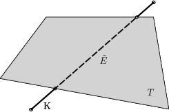
(a)

(b)

Figure 4: Triangulation of the intersected region $\tilde{E}$ for a line immersed in 2D. The one-dimensional cell $K$ is allowed to be positioned arbitrarily w.r.t. to the two-dimensional quadrilateral $T$.

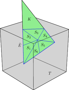
(a)

(b)

Figure 5: Triangulation of the intersected region $\tilde{E}$ for a triangle cutting a square and the relative sub-tessellation.

4.3 Integration through level set splitting

If a level set description of the immersed domain is available, this may be used to generate quadrature formulas without explicitly computing the geometric intersection (see [10] for some implementation details). It has also been shown in [26] how to generate quadrature rules on different regions of a cut element using $\Psi$, identified as

$$O=\{(x,y)\in T:\Psi>0\},$$

$$S=\{(x,y)\in T:\Psi=0\},$$

$$I=\{(x,y)\in T:\Psi<0\},$$

where $\Psi:\mathbb{R}^{d}\rightarrow\mathbb{R}$ is the level set function determining the immersed domain. A typical configuration including quadrature points for each entity is shown in Figure 6.

(a)

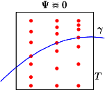
(b)

(c)

Figure 6: Quadrature points distributed on $O$, $S$ and $I$ for a cell $T$ cut by the curve $\gamma$.

In practical computations, however, the interface $\gamma$ is not available in terms of a simple analytical description of the level set function. Should one still wish to use quadrature formulas based on a level set, a discrete (possibly approximated) level set function $\Psi_{h}$ that is zero on $\gamma_{h}$ must be provided when $\gamma_{h}$ is a triangulated surface. Such level set would also allow a robust partitioning of the background computational mesh into cells that are completely inside $\omega$, cells cut by $\gamma$, and cells that are completely inside $\Omega\setminus\omega$.

We propose a simple implementation of a discrete level set function $\Psi_{h}$ constructed from a triangulated interface $\gamma_{h}$. Point classification (i.e., detecting if a point is inside or outside $\omega$) is performed using a query to the CGAL library, to detect if a point is inside or outside the coarsest simplicial mesh bounded by $\gamma_{h}$ (denoted by $\mathcal{I}_{h}$).

We then define a discrete level set function $\Psi_{h}(\boldsymbol{x})$ on top of $\gamma_{h}$ as follows:

$$\Psi_{h}(\boldsymbol{p})=\begin{cases}-d(\boldsymbol{p},\gamma)&\text{if }\boldsymbol{p}\in\mathcal{I}_{h},\\ d(\boldsymbol{p},\gamma)&\text{if }\boldsymbol{p}\notin\mathcal{I}_{h},\\ \end{cases}$$

where $d(\boldsymbol{p},\gamma)\coloneqq\min_{\boldsymbol{y}\in\gamma}d(\boldsymbol{p},\boldsymbol{y})$ is constructed by first finding the closest elements of $\gamma$ to $\boldsymbol{p}$ using efficient R-tree data structures indexing the cells of the immersed triangulation, and then computing the distance between $\boldsymbol{p}$ and those elements.

This procedure is summarized in Algorithm 1. We validate our approach with a manufactured case by choosing randomly distributed points $\{p_{i}\}_{i}$ in the interval $[-1,1]^{2}$ and computing the relative error $E_{r}(\boldsymbol{p})\coloneqq\frac{|\Psi(\boldsymbol{p})-\Psi_{h}(\boldsymbol{p})|}{|\Psi(\boldsymbol{p})|}$ for a level set describing a circle of radius $R=0.3$, and a corresponding approximated grid $\gamma_{h}$.

In Figure 7 we report the relative error committed by replacing the exact level set with the discrete one (induced by replacing the exact curve with a triangulated one). The initial discretization of $\gamma$ is chosen so that the error is below $10^{-6}$ everywhere, and we can safely neglect it when computing convergence rates of the error computed w.r.t. exact solutions known on the analytical level set.

As long as such geometrical error is not dominating we can observe optimal rates in the numerical experiments for cut-FEM. At the same time, this setting allows for a fair comparison between all the schemes. We expect that other practical implementations would require similar tasks and hence that the observed computational cost is representative.

Figure 7: The relative error for the discrete level set describing a disk of radius $R=0.3$ as a function of the distance from the center $\boldsymbol{x_{c}}=(\frac{1}{2},\frac{1}{2})$.

Input : $\gamma$ polygonal surface mesh,

$\mathcal{I}_{h}$ coarse triangulation for the interior of $\gamma$,

$\boldsymbol{p}\in\Omega$.

Output : $d(\boldsymbol{p},\gamma)$.

1 if $\boldsymbol{p}\in\mathcal{I}_{h}$ then

2       $s\leftarrow-1$

3else

4       $s\leftarrow+1$

5 end if

6$\text{Find}\{K_{i}\}\in\gamma_{h}\text{ nearest to }\boldsymbol{p}$.

7 for $K\in\{K_{i}\}_{i}$ do

8       $d_{i}\leftarrow d(\boldsymbol{p},K)$;

9 end for

$\text{Return }s\cdot\min_{i}d_{i}$

Algorithm 1 Evaluation of the discrete level set (4.3) for a given mesh $\gamma$.

5 Numerical experiments

Our implementation is based on the C++ finite element library deal.II [2, 1], providing a dimension independent user interface. The implementation of the Lagrange multiplier and of the Nitsche’s interface penalization methods are adapted from the tutorial programs step-60 and step-70 of the deal.II library, respectively, while the cut-FEM algorithm is adapted from the tutorial program step-85, developed in [28].

As a result of this work, we added support and wrappers for the C++ library CGAL ([29], [13]) into the deal.II library [2], in order to perform most of the computational geometry related tasks. Thanks to the so called exact computation paradigm provided by CGAL, which relies on computing with numbers of arbitrary precision, our intersection routines are guaranteed to be robust.

We assume that the background mesh $\Omega_{h}$ is a $d$-dimensional triangulation and the immersed mesh $\gamma_{h}$ is $(d-1)$-dimensional with $d=2,3$. We validate our implementations with several experiments varying mesh configurations, algorithms, and boundary conditions. The source code used to reproduce the numerical experiments is available from GitHub .

The tests are designed to analyze the performance of the methods presented in Section 3 in different settings, varying the complexity of the interface and the smoothness of the exact solution in both two and three dimensions. All tests are performed using background meshes made of quadrilaterals or hexahedra and immersed boundary meshes made of segments and quadrilaterals. For the Lagrange multiplier and Nitsche’s interface penalization methods, we perform an initial pre-processing of the background grid $\Omega$ by applying a localized refinement around the interface (where most of the error is concentrated), so that the resulting number of degrees of freedom for the variable $u_{h}$ is roughly the same for all methods. Sample grids resulting from this process are shown in Figure 8, where the interface has been resolved from $\Omega_{h}$. We then proceed by computing errors and convergence rates against a manufactured solution under simultaneous refinement of both the background and immersed mesh.

Classical $\mathcal{Q}^{1}$ Lagrangian elements are used for the background space while piecewise constant elements are used to discretize the Lagrange multiplier. For the Nitsche penalization method (20), we set the penalty parameter as $\beta=10$. Errors in the $H^{1}$- and $L^{2}$-norm are reported for the main variable while for the Lagrange multiplier we use the discrete norm in (7) which, as already observed, is equivalent to the $H^{-1/2}(\gamma)$ norm on a quasi-uniform mesh. In the case of the Lagrange multiplier method, we report the sum of the number of Degrees of Freedom (DoF) for $u_{h}$ and $\lambda_{h}$ to underline the fact that a larger system must be solved, while rates are computed against the number of DoF of each unknown.

For the (symmetric) penalized methods, the resulting linear systems are solved using a preconditioned conjugate gradient method, with an algebraic multigrid preconditioner based on the Trilinos ML implementation [19], while for the Lagrange multiplier we exploit the preconditioner described in Section 3.1 with the same preconditioned conjugate gradient method for inner solves of the stiffness matrices, and flexible GMRES as the outer solver. In the case of the Lagrange multiplier method, we list the total number of inner iterations required to invert the Schur complement.

5.1 2D numerical tests

In order to make the comparison between the three methods as close to real use cases as possible, we do not exploit any a-priori knowledge of analytical level set descriptions of the exact interfaces. Indeed, using this information one could expect faster computations of the intersections, and an overall reduction of the computational costs of the assembly routines. Instead, we fix the same discretization of the interface as input data of the computational problem for all three methods.

In particular, we consider as computational domain $\Omega=[-1,1]^{2}$ with immersed domains of different shapes originating from an unfitted discretization of two different curves:

• circle interface; we let $\gamma^{1}\coloneqq\partial B_{R}(\boldsymbol{c})$,

• flower-shaped interface; we let $\gamma^{2}\coloneqq\Bigl{\{}(x,y):\sqrt{x^{2}+y^{2}}-r\Bigl{(}1-2\frac{y^{2}}{x^{2}+y^{2}}\Bigr{)}\Bigl{(}1-16\frac{x^{2}y^{2}}{(x^{2}+y^{2})^{2}}\Bigr{)}-R=0\Bigr{\}}$,

where the first is a circle of radius $R$ centered at $\boldsymbol{c}$ and the second is a flower-like interface. We choose as parameter values $\boldsymbol{c}=(\frac{1}{2},\frac{1}{2})$, $R=0.3$ and $r=0.1$. The initial discretization of the immersed domains are chosen so that the geometrical error is negligible w.r.t. the discretization errors (see Figure 8). In the case of the circle interface $\gamma^{1}$, the discrete interface is generated using a built-in mesh generatorsfrom deal.II while the flower-shaped interface $\gamma^{2}$ is imported from an external file. When required, we implement a discrete level set function $\Psi_{h}$ as described in Algorithm 1. Figure 8 shows a representation of the two interfaces.

In the first two tests, we set up the problem using the method of manufactured solutions, imposing the data $f$ in $\Omega$ and the boundary conditions on $\Gamma$ and $\gamma$ according to the exact solution

$$u(x,y)\coloneqq\sin(2\pi x)\sin(2\pi y).$$ (30)

Hence, the right hand side of (1) is $f=8\pi^{2}u(x,y)$ and the data on the outer boundary $\Gamma$ and on $\gamma$ are computed accordingly. Notice that the smoothness of the solution implies $\lambda\equiv 0$ in this case.

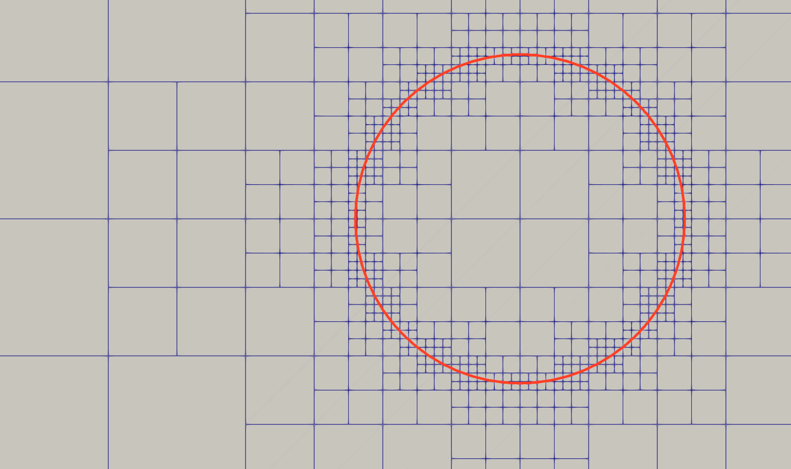
(a)

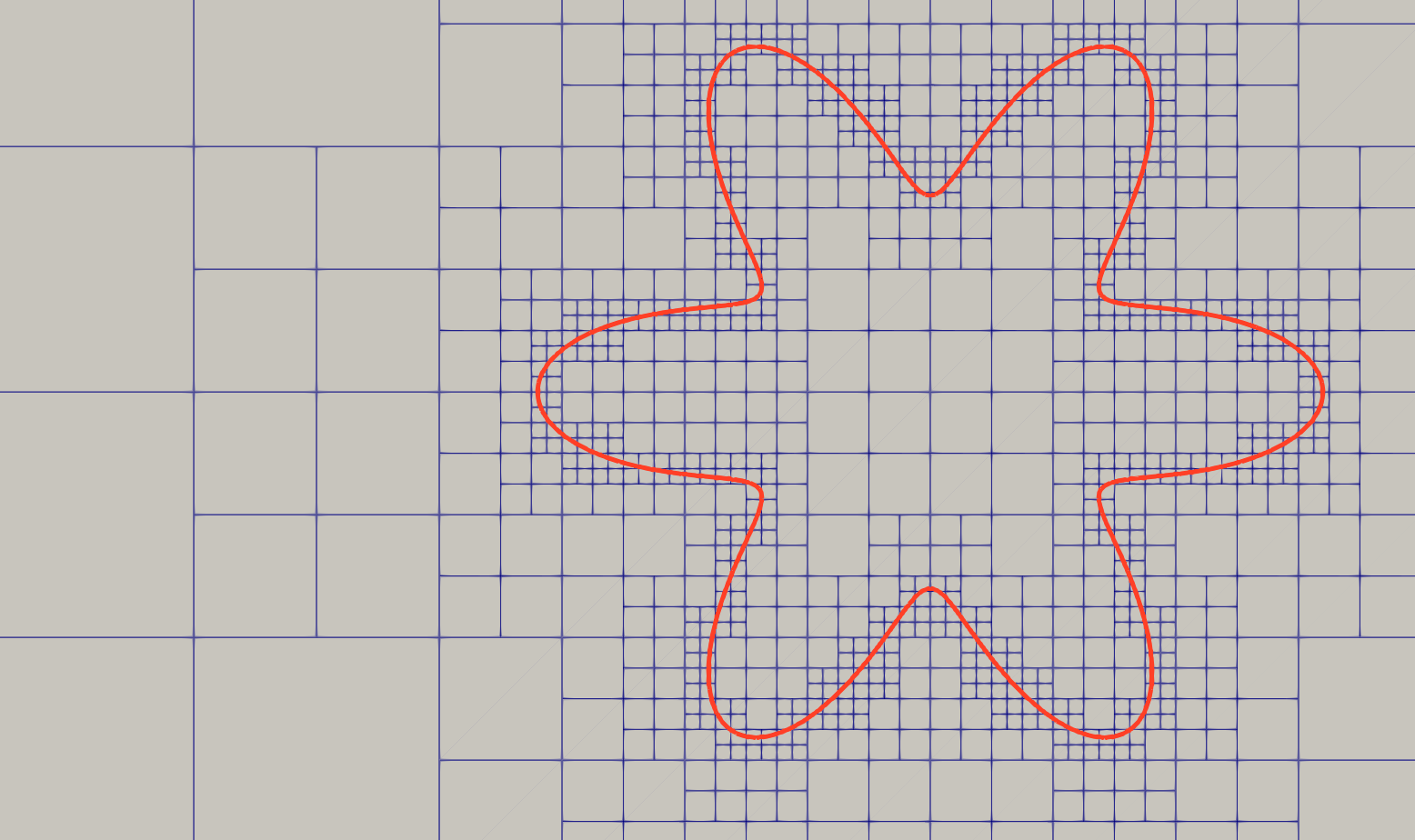
(b)

Figure 8: Zoom on pre-processed background grid $\Omega_{h}$ for the circle interface $\gamma=\gamma^{1}$ (left) and the flower-shaped interface $\gamma=\gamma^{2}$ (right).

This test is meant to assess the basic correctness of the implementation of the three methods, and corresponds to a case in which the interface is truly not an interface.Instead, when we impose an arbitrary value for the solution at the interface, we expect the solution $u$ to be only in $H^{\frac{3}{2}-\varepsilon}(\Omega)$ for any $\varepsilon>0$, even thought its local regularity on the two subdomains $\omega$ and $\Omega\setminus\omega$ may be higher. This is due to the fact that the gradient of the solution is not a continuous function across the interface, and therefore the solution cannot be in $H^{2}(\Omega)$. In this case, we cannot expect non-matching methods that does not resolve the interface exactly, such as the Lagrange multiplier and the Nitsche’s interface penalization method, to be able to recover the optimal rate of convergence.

In the tables below we also report the number of iterations required in the solution phase in the column ‘Iter.’. We observe for all experiments a similar number of iterations for the three methods (which are independent on the number of degrees of freedom, indicating a good choice of preconditioner for all three methods) even though the solution of the linear system stemming from the Lagrange multiplier method is generally more expensive compared to the other two methods, owing to the higher computational complexity of the preconditoner for the saddle-point problem. The balance in the computational cost of the three different methods is discussed in details in Section 5.3.

5.1.1 Test 1: smooth solution over circular interface

We report in Tables 1, 2, and 3 the errors and computed rates for the Lagrange multiplier, Nitsche’s interface penalization, and cut-FEM method, respectively. In each case, the background variable converges linearly and quadratically in the $H^{1}$- and $L^{2}$-norm, respectively. As for the Lagrange multiplier, we observe a convergence rate close to two instead of the theoretical rate of one, most likely due to the very special exact solution that the multiplier converges to (i.e., the zero function). For a direct comparison, we also report in Figure 9 (left) the convergence history of all three methods against the number of DoF. These results clearly indicate that for smooth problems with relatively simple interfaces the three methods perform similarly.

Results for $\gamma=\gamma^{1}$ and smooth solution with Lagrange multiplier
DoF number	$\|u-u_{h}\|_{0,\Omega}$	$L^{2}(\Omega)$ rate	$\|u-u_{h}\|_{1,\Omega}$	$H^{1}(\Omega)$ rate	$\|\lambda-\lambda_{h}\|_{-\frac{1}{2},\gamma}$	$H^{-\frac{1}{2}}(\gamma)$ rate	Iter.
389+32	5.579e-02	-	1.879e+00	-	7.402e-02	-	7
1721+64	1.393e-02	1.87	9.391e-01	0.93	1.042e-02	2.83	7
7217+128	3.479e-03	1.94	4.690e-01	0.97	2.805e-03	1.89	9
29537+256	8.691e-04	1.97	2.343e-01	0.98	6.716e-04	2.06	11
119489+512	2.172e-04	1.98	1.171e-01	0.99	2.078e-04	1.69	11

Table 1: Rates in $L^{2}$ and $H^{1}$ for a smooth $u$ and $H^{-\frac{1}{2}}$ rates for the Lagrange multiplier method.

Results for $\gamma=\gamma^{1}$ and smooth solution with Nitsche
DoF number	$\|u-u_{h}\|_{0,\Omega}$	$L^{2}(\Omega)$ rate	$\|u-u_{h}\|_{1,\Omega}$	$H^{1}(\Omega)$ rate	Iter.
389	5.597e-02	-	1.879e+00	-	1
1721	1.396e-02	2.13	9.391e-01	1.06	11
7217	3.487e-03	2.06	4.690e-01	1.03	11
29537	8.712e-04	2.03	2.343e-01	1.02	12
119489	2.177e-04	2.02	1.171e-01	1.01	12

Table 2: $L^{2}$ and $H^{1}$ error rates for $\gamma=\gamma^{1}$ and a smooth solution with Nitsche.

Results for $\gamma=\gamma^{1}$ and smooth solution with cut-FEM
DoF number	$\|u-u_{h}\|_{0,\Omega}$	$L^{2}(\Omega)$ rate	$\|u-u_{h}\|_{1,\Omega}$	$H^{1}(\Omega)$ rate	Iter.
329	8.7560e-02	-	2.1335e+00	-	2
1161	2.2064e-02	1.99	1.0582e+00	1.01	2
4377	5.4875e-03	2.01	5.2351e-01	1.02	15
16953	1.3554e-03	2.02	2.5863e-01	1.02	17
66665	3.3152e-04	2.03	1.2855e-01	1.01	18

Table 3: $L^{2}$ and $H^{1}$ error rates for $\gamma=\gamma^{1}$ and a smooth solution with cut-FEM.

5.1.2 Test 2: smooth solution over flower-shaped interface

We report in Tables (4), (5) and (6) the error with the computed rates of convergence for the three schemes. Again we observe the theoretical rates of convergence for all three methods. This time, however, the direct comparison of the errors shown in Figure 9 (right) indicates that the cut-FEM approach has an advantage over the other two methods. This may be due to the worst approximation properties of the non-matching methods based on Lagrange multipliers and Nitsche’s interface penalization in the presence of high curvature sections of the immersed boundary, as can be seen by comparing the meshes shown in Figure 8. Despite the fact that the reached accuracy is the same for the Lagrange multiplier and We further note that the Nitsche’s interface penalization method requires less iterations than the Lagrange multiplier method.

Figure 9: $L^{2}$, $H^{1}$, and $H^{-\frac{1}{2}}$ errors versus the number of DoF for all schemes applied to $\gamma^{1}$ (left) and to $\gamma^{2}$ (right).

Results for $\gamma=\gamma^{2}$ and smooth solution with Lagrange multiplier
DoF number	$\|u-u_{h}\|_{0,\Omega}$	$L^{2}(\Omega)$ rate	$\|u-u_{h}\|_{1,\Omega}$	$H^{1}(\Omega)$ rate	$\|\lambda-\lambda_{h}\|_{-\frac{1}{2},\gamma}$	$H^{-\frac{1}{2}}(\gamma)$ rate	Iter.
1958+256	5.327e-02	-	1.781e+00	-	6.551e-03	-	17
8783+512	1.331e-02	1.85	8.916e-01	0.92	1.183e-03	2.47	20
37037+1024	3.326e-03	1.93	4.458e-01	0.96	5.237e-04	1.18	33
151961+2048	8.312e-04	1.96	2.228e-01	0.98	1.959e-04	1.42	49
615473+4096	2.078e-04	1.98	1.114e-01	0.99	5.327e-05	1.88	53

Table 4: $L^{2}$ and $H^{1}$ error rates for $\gamma=\gamma^{2}$ and a smooth solution with Lagrange multiplier method.

Results for $\gamma=\gamma^{2}$ and smooth solution with Nitsche
DoF number	$\|u-u_{h}\|_{0,\Omega}$	$L^{2}(\Omega)$ rate	$\|u-u_{h}\|_{1,\Omega}$	$H^{1}(\Omega)$ rate	Iter.
1958	5.327e-02	-	1.781e+00	-	13
8783	1.331e-02	1.85	8.916e-01	0.92	12
37037	3.326e-03	1.93	4.458e-01	0.96	13
151961	8.312e-04	1.96	2.228e-01	0.98	12
615473	2.078e-04	1.98	1.114e-01	0.99	14

Table 5: $L^{2}$ and $H^{1}$ error rates for $\gamma=\gamma^{2}$ and a smooth solution with Nitsche

Results for $\gamma=\gamma^{2}$ and smooth solution with cut-FEM
DoF number	$\|u-u_{h}\|_{0,\Omega}$	$L^{2}(\Omega)$ rate	$\|u-u_{h}\|_{1,\Omega}$	$H^{1}(\Omega)$ rate	Iter.
1209	2.2306e-02	-	1.0422e+00	-	2
4487	5.7207e-03	1.96	5.2424e-01	0.99	17
17163	1.4123e-03	2.02	2.5901e-01	1.02	17
67089	3.4377e-04	2.04	1.2865e-01	1.01	19
265249	8.5223e-05	2.01	6.4118e-02	1.00	20

Table 6: $L^{2}$ and $H^{1}$ error rates for $\gamma=\gamma^{2}$ and a smooth solution with cut-FEM

5.1.3 Test 3: non-smooth solution over circular interface

In this test, we fix once more $\gamma=\gamma^{1}$ and we define an exact solution with a non-zero jump of the normal gradient $\nabla u\cdot\boldsymbol{n}$ across $\gamma$ taken from [18], namely

$$u(x,y) =\begin{cases}-\ln(R)\qquad\text{if }|r|\leq R\\ -\ln(r)\qquad\text{ if }|r|>R,\\ \end{cases}$$ (31)

where $r\coloneqq\boldsymbol{x}-\boldsymbol{c}$, implying as right hand side $f=0$. The Lagrange multiplier associated to this solution is $\lambda(\boldsymbol{x})\equiv\lambda=-\frac{1}{R}$, as $u$ solves the following classical interface problem:

$$\begin{cases}-\Delta u&=0\qquad\text{ in }\Omega\setminus\gamma,\\ u&=-\ln(r)\quad\text{ on }\Gamma,\\ \llbracket\nabla u\cdot\boldsymbol{n}\rrbracket&=\frac{1}{R}\quad\text{ on }\gamma,\\ \llbracket u\rrbracket&=0\quad\text{ on }\gamma.\\ \end{cases}$$ (32)

Since the global regularity of the solution is $H^{\frac{3}{2}-\varepsilon}(\Omega)$ for any $\varepsilon>0$, theoretically we would expect the convergence rates of the $L^{2}(\Omega)$, $H^{1}(\Omega)$, and $H^{-\frac{1}{2}}(\gamma)$ norms of the errors to be $1$, $0.5$, and $0.5$ for the Lagrange multiplier method, the same for the variable $u_{h}$ in the Nitsche’s interface penalization method, and the optimal convergence rates observed in the smooth case in the case of the cut-FEM method. These are shown in Tables 7, 8 and 9 and plotted in Figure 10.

The results show a clear advantage in terms of convergence rates and absolute values of the errors for the cut-FEM method. In all cases (both smooth and non-smooth), the Nitsche’s interface penalization method and the Lagrange multiplier give essentially the same errors. A simple way to improve the situation for the latter two methods would be to use a weighted norm during the computation of the error, which was proven to be localized at the interface in [18]. This would allow to reduce the overall error, but it would still result in a solution that does not capture correctly the jump of the normal gradient across the interface, which is the main source of error.

Results for $\gamma=\gamma^{1}$ and non-smooth solution with Lagrange multipliers
DoF number	$\|u-u_{h}\|_{0,\Omega}$	$L^{2}(\Omega)$ rate	$\|u-u_{h}\|_{1,\Omega}$	$H^{1}(\Omega)$ rate	$\|\lambda-\lambda_{h}\|_{-\frac{1}{2},\gamma}$	$H^{-\frac{1}{2}}(\gamma)$ rate	Iter.
389+32	1.413e-02	-	3.656e-01	-	3.354e-02	-	2
1721+64	5.706e-03	1.39	2.254e-01	0.74	1.112e-02	1.59	14
7217+128	3.250e-03	0.84	1.621e-01	0.49	6.273e-03	0.83	13
29537+256	1.796e-03	0.87	1.141e-01	0.51	4.094e-03	0.62	15
119489+512	1.099e-03	0.71	8.015e-02	0.51	2.845e-03	0.52	14

Table 7: $L^{2}$-error and $H^{1}$-error for non smooth $u$ in (31) and for the multiplier.

Results for non-smooth $u$ with Nitsche
DoF number	$\|u-u_{h}\|_{0,\Omega}$	$L^{2}(\Omega)$ rate	$\|u-u_{h}\|_{1,\Omega}$	$H^{1}(\Omega)$ rate	Iter.
389	9.216e-03	-	3.667e-01	-	1
1721	3.324e-03	1.37	2.286e-01	0.64	11
7217	1.936e-03	0.75	1.640e-01	0.46	11
29537	9.957e-04	0.94	1.151e-01	0.50	12
119489	5.016e-04	0.98	8.070e-02	0.51	13

Table 8: $L^{2}$-error, $H^{1}$-error for non smooth $u$ in (31).

Results for non-smooth $u$ with cut-FEM
DoF number	$\|u-u_{h}\|_{0,\Omega}$	$L^{2}(\Omega)$ rate	$\|u-u_{h}\|_{1,\Omega}$	$H^{1}(\Omega)$ rate	Iter.
329	3.1670e-02	-	5.6660e-01	-	2
1161	1.5998e-03	4.31	1.2352e-01	2.20	2
4377	3.6791e-04	2.12	5.8327e-02	1.08	16
16953	8.5282e-05	2.11	2.7307e-02	1.09	18
66665	2.1914e-05	1.96	1.3726e-02	0.99	19

Table 9: $L^{2}$-error, $H^{1}$-error for non smooth $u$ in (31) with cut-FEM.

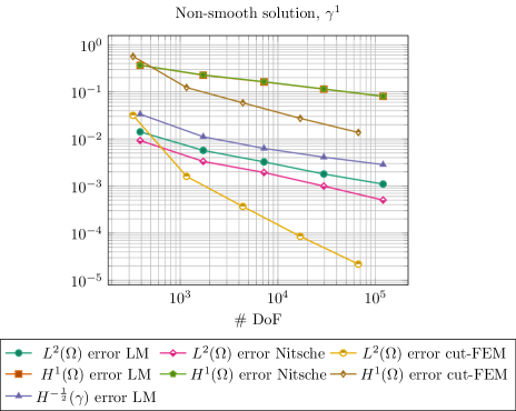
Figure 10: $L^{2}$, $H^{1}$, and $H^{-\frac{1}{2}}$ errors versus the number of DoF for all schemes applied to $\gamma^{1}$, with non-smooth solution.

5.2 3D numerical tests

We mimic the tests reported above for the two-dimensional setting also in the three-dimensional case, but we restrict our analysis to the case of a sphere immersed in a box. We fix $\Omega=[-1,1]^{3}$ and consider as immersed interface a sufficiently fine discretization of the sphere $\gamma^{3}\coloneqq\partial B_{R}(\boldsymbol{c})$ with $\boldsymbol{c}=(\frac{1}{2},\frac{1}{2},\frac{1}{2})$, $R=0.3$. In this setting, we consider two test cases with smooth and non-smooth solution.

5.2.1 Test 1: smooth solution over spherical interface

We proceed analogously to the previous section by computing convergence rates when the solution $u$ is smooth and defined as

$$u(x,y,z)\coloneqq\sin(2\pi x)\sin(2\pi y)\sin(2\pi z),$$ (33)

which corresponds to the right hand side $f=12\pi^{2}u(x,y,z)$. We report in Tables 10, 11 and 12 the error rates for the three schemes, while in Figures 11 (left) we plot errors against the number of DoF.

The convergence rates are as expected and the results are in line with the two-dimensional case. The Lagrange multiplier method and the interface penalization method give again very close computational errors for $u_{h}$. As in the smooth two-dimensional case, this test should only be considered as a validation of the code and of the error computation, since the interface does not have any effect on the computational solutions.

Results for $\gamma=\gamma^{3}$ and smooth solution with Lagrange multiplier
DoF number	$\|u-u_{h}\|_{0,\Omega}$	$L^{2}(\Omega)$ rate	$\|u-u_{h}\|_{1,\Omega}$	$H^{1}(\Omega)$ rate	$\|\lambda-\lambda_{h}\|_{-\frac{1}{2},\gamma}$	$H^{-\frac{1}{2}}(\gamma)$ rate	Iter.
4127+96	6.416e-02	-	2.432e+00	-	0.1027	-	9
37031+384	1.590e-02	1.91	1.212e+00	0.95	0.0287	1.84	18
313007+1536	3.963e-03	1.95	6.051e-01	0.98	0.0069	2.06	19
2572511+6144	9.996e-04	1.96	3.024e-01	0.99	0.0019	1.89	14

Table 10: $L^{2}$ and $H^{1}$ error rates for $\gamma=\gamma^{3}$ and a smooth solution with Lagrange multiplier.

Results for $\gamma=\gamma^{3}$ and smooth solution with Nitsche
DoF number	$\|u-u_{h}\|_{0,\Omega}$	$L^{2}(\Omega)$ rate	$\|u-u_{h}\|_{1,\Omega}$	$H^{1}(\Omega)$ rate	Iter.
4127	6.411e-02	-	2.432e+00	-	17
37031	1.588e-02	2.01	1.212e+00	1.00	14
313007	3.959e-03	2.00	6.050e-01	1.00	14
2572511	9.887e-04	2.00	3.023e-01	1.00	14

Table 11: $L^{2}$ and $H^{1}$ error rates for $\gamma=\gamma^{3}$ and a smooth solution with Nitsche.

Results for $\gamma=\gamma^{3}$ and smooth solution with cut-FEM
DoF number	$\|u-u_{h}\|_{0,\Omega}$	$L^{2}(\Omega)$ rate	$\|u-u_{h}\|_{1,\Omega}$	$H^{1}(\Omega)$ rate	Iter.
5163	7.0847e-02	-	2.4835e+00	-	13
36781	1.7743e-02	2.12	1.2479e+00	1.05	12
278157	4.5124e-03	2.03	6.2396e-01	1.03	13
2160541	1.1302e-03	2.03	3.1154e-01	1.02	13

Table 12: $L^{2}$ and $H^{1}$ error rates for $\gamma=\gamma^{3}$ and a smooth solution with cut-FEM

5.2.2 Test 2: non-smooth solution over spherical interface

We consider the test case in [18]:

$$u(x,y) =\begin{cases}\frac{1}{R}&\text{ if }|r|\leq R,\\ \frac{1}{|r|}&\text{if }|r|>R,\\ \end{cases}$$ (34)

where $r\coloneqq\boldsymbol{x}-\boldsymbol{c}$, $f=0$, and $R=0.3$. Analogously to the two dimensional case, the multiplier associated to this problem is $\lambda(\boldsymbol{x})=\lambda=-\frac{1}{R^{2}}$, since $u$ solves the following problem:

$$\begin{cases}-\Delta u&=0\qquad\text{ in }\Omega\setminus\gamma,\\ u&=\frac{1}{|r|}\quad\text{ on }\Gamma,\\ \llbracket\nabla u\cdot\boldsymbol{n}\rrbracket&=\frac{1}{R^{2}}\quad\text{ on }\gamma,\\ \llbracket u\rrbracket&=0\quad\text{ on }\gamma.\\ \end{cases}$$ (35)

We report in Tables 13, 14, 15 the error rates for the three schemes and in Figure 11 (right) the error decay in $L^{2}(\Omega)$ and $H^{1}(\Omega)$ for $u_{h}$ and the decay in $H^{-\frac{1}{2}}(\gamma)$ for $\lambda_{h}$. A contour plot of the discrete solution $u_{h}$ obtained with Nitsche’s penalization method is shown in Figure 12.

The difference between the three methods is less evident in terms of absolute values of the errors when compared to the two dimensional case: while it is still clear that the convergence rates of cut-FEM are higher compared to the other two methods, the difference between the three methods is smaller. In particular, the Nitsche’s interface penalization method seems to perform better than the Lagrange multiplier method when considering the $L^{2}$ norm.

Results for $\gamma=\gamma^{3}$ and non-smooth solution with Lagrange multiplier
DoF number	$\|u-u_{h}\|_{0,\Omega}$	$L^{2}(\Omega)$ rate	$\|u-u_{h}\|_{1,\Omega}$	$H^{1}(\Omega)$ rate	$\|\lambda-\lambda_{h}\|_{-\frac{1}{2},\gamma}$	$H^{-\frac{1}{2}}(\gamma)$ rate	Iter.
4127+96	3.907e-02	-	1.251e+00	-	0.4552	-	2
37031+384	2.041e-02	0.89	8.119e-01	0.59	0.2598	0.81	3
313007+1536	1.095e-02	0.88	5.764e-01	0.48	0.1806	0.52	3
2572511+6446	6.214e-03	0.81	4.253e-01	0.43	0.1216	0.57	3

Table 13: $L^{2}$ and $H^{1}$ error rates for $\gamma=\gamma^{3}$ and non-smooth solution $u$ in 34 with Lagrange multiplier.

Results for $\gamma=\gamma^{3}$ and non-smooth solution with Nitsche
DoF number	$\|u-u_{h}\|_{0,\Omega}$	$L^{2}(\Omega)$ rate	$\|u-u_{h}\|_{1,\Omega}$	$H^{1}(\Omega)$ rate	Iter.
4127	8.688e-02	-	1.562e+00	-	19
37031	2.157e-02	2.01	8.885e-01	0.81	16
313007	4.893e-03	2.14	5.724e-01	0.63	16
2572511	1.887e-03	1.37	3.954e-01	0.53	16

Table 14: Rates for $\gamma=\gamma^{3}$ and a non-smooth solution $u$ in 34 with Nitsche.

Results for $\gamma=\gamma^{3}$ and non-smooth solution with cut-FEM
DoF number	$\|u-u_{h}\|_{0,\Omega}$	$L^{2}(\Omega)$ rate	$\|u-u_{h}\|_{1,\Omega}$	$H^{1}(\Omega)$ rate	Iter.
5163	6.3609e-02	-	1.3046e+00	-	25
36781	6.9076e-03	3.39	4.5097e-01	1.62	22
278157	1.5076e-03	2.26	2.2098e-01	1.06	24
2160541	3.3802e-04	2.19	9.3590e-02	1.26	24

Table 15: $L^{2}$ and $H^{1}$ error for $\gamma=\gamma^{3}$ and a non-smooth solution $u$ in 34 with cut-FEM

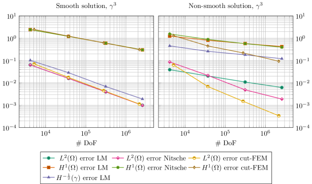
Figure 11: $L^{2}$, $H^{1}$, and $H^{-\frac{1}{2}}$ error versus the number of DoF for all schemes applied to $\gamma^{3}$ with a smooth solution $u$ (left) and with a non-smooth solution $u$ (right).

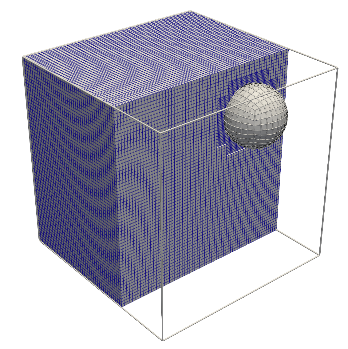
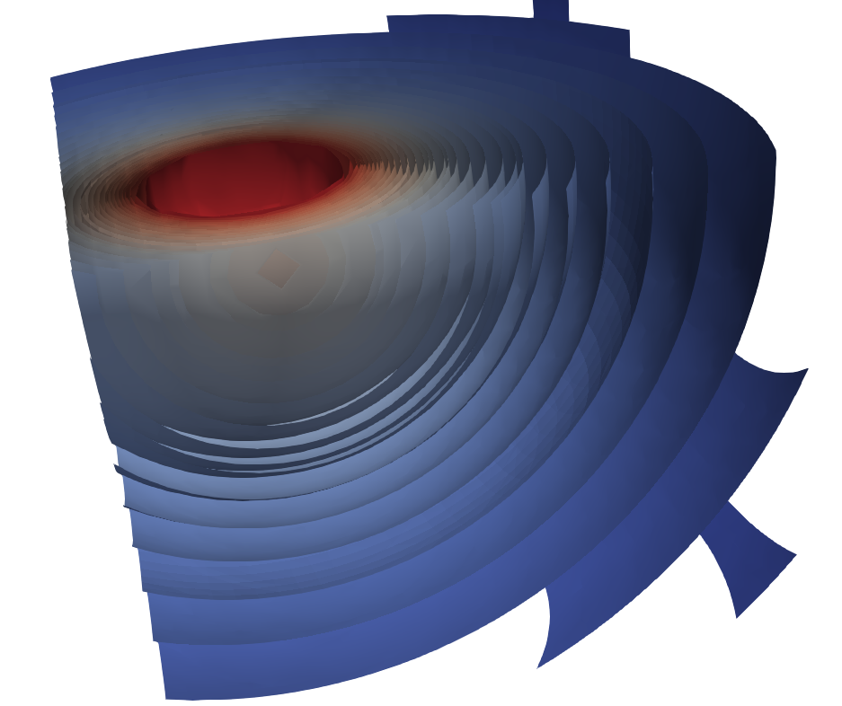
Figure 12: Background mesh $\Omega_{h}$ and immersed mesh of the sphere interface $\gamma_{h}$ for the three dimensional case (left) and section of the contour plot for the approximate solution $u_{h}$ in (34), $\gamma=\gamma^{3}$.

5.3 Computational times

In order to better understand the performance of the three methods, we consider a breakdown of the computational costs into work precision diagrams. These provide a more fair measure of efficiency as they take into account the computational cost required to reach a given accuracy.

We report hereafter a breakdown of the computational times needed by our implementations of the three proposed methods. All computations were carried out on a 2.60GHz Intel Xeon processor. For each benchmark we report the average time required to solve 10 times the 3D smooth Problem 5.2.1. We compute separately the required CPU times (in seconds) for the main tasks that each scheme has to perform. On a quasi-uniform mesh, the number $N$ of background cells in $\Omega_{h}$ scales with $\mathcal{O}(h_{\Omega}^{-3})$, and we expect the assembly of the stiffness matrix to scale linearly in the number of cells. On the other hand, the number of facets in $\gamma_{h}$ scales with $\mathcal{O}(h_{\gamma}^{-2})$; in our experiments, the ratio $h_{\Omega}/h_{\gamma}$ is kept fixed, therefore we expect the assembly of the coupling terms $\langle\lambda,v\rangle_{\gamma}$ and $\langle u,v\rangle_{\gamma}$ to scale with $\mathcal{O}(N^{\frac{2}{3}})$.

This is indeed what we observe in the experiments as shown in CPU breakdown plots of Figure 13 for each method.

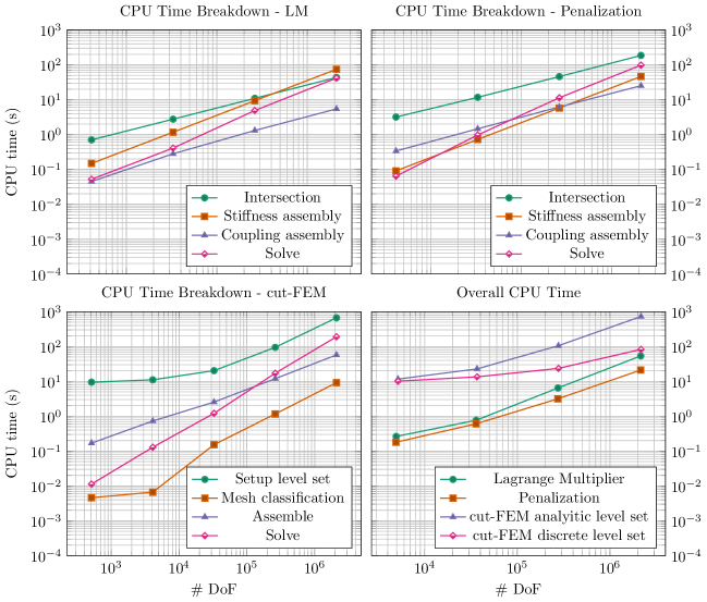
Figure 13: Breakdown of CPU times for the three schemes. In (bottom left) Setup level set indicates the time required to interpolate the discrete level set described in Algorithm 1 onto the finite element space. Mesh classification shows the time needed to partition the computational mesh and classify the cells in cut, interior or outside cells. Bottom right: overall CPU times to assemble the algebraic system for the smooth 3D test. For the cut-FEM method, we also show the CPU time obtained by using an analytical representation of the interface through an analytic level set function.

The three schemes have comparable computational times. In particular, the Nitsche interface penalization method exhibits lower global assembly times compared to the others. However, it is well known that the number of iterations required to solve the algebraic problem is influenced by the choice of the penalty parameter $\beta$ in (20), which determines simultaneously also the accuracy of the numerical solution $u_{h}$. This can be better seen in work-precision diagrams, where we compare the CPU times to solve each refinement cycle versus the $L^{2}$ error for both test problems (33) and (34) in Figure 14. In the smooth scenario, results for the Lagrange multiplier and Nitsche’s interface penalization methods are almost overlapping both in terms of time and accuracy, while cut-FEM shows larger computational times. The situation is different in the non-smooth case where cut-FEM better captures the discontinuity at the interface and thus gives more accurate results, with a larger cost in terms of time for low degrees of freedom count, and with smaller cost for large degrees of freedom count, owing to the better convergence rate of the method. These results indicate that the additional implementation complexity does pay back for non-smooth solutions.

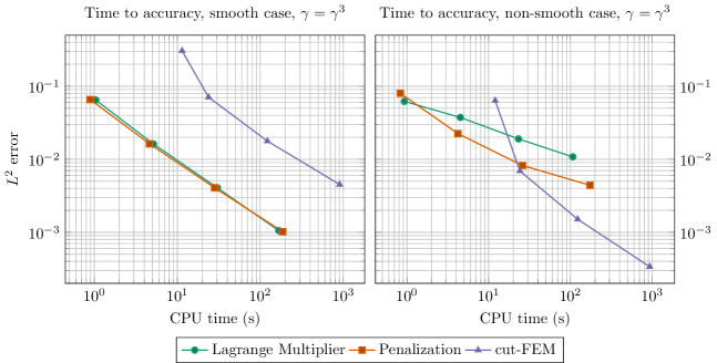
Figure 14: Work-precision diagrams for the two 3D tests.

Based on the higher efficiency of the Lagrange multiplier and Nitsche penalization method in the smooth case, we speculate that these methods can be made competitive also in the non-smooth case by an improved local refinement strategy [17].

6 Conclusions

The numerical solution of partial differential equations modeling the interaction of physical phenomena across interfaces with complex, possibly moving, shapes is of great importance in many scientific fields. Boundary unfitted methods offer a valid alternative to remeshing and Arbitrary Lagrangian Eulerian formulations, but require care in the representation of the coupling terms between the interface and the bulk equations.

In this work, we performed a comparative analysis of three non-matching methods, namely the Lagrange multiplier method (or fictitious domain method), the Nitsche’s interface penalization method, and the cut-FEM method, in terms of accuracy, computational cost, and implementation effort.

We presented the major algorithms used to integrate coupling terms on non-matching interfaces, discussed the benefit of computing accurate quadrature rules on mesh intersections, and concluded our analysis with a set of numerical experiments in two and three dimensions.

Our results show that accurate quadrature rules can significantly improve the accuracy of the numerical methods, and that there are cases in which simpler methods, like the Nitsche’s interface penalization method, are competitive in terms of accuracy per computational effort. In general, the additional implementation burden of the cut-FEM method is justified by the higher accuracy that it achieves, even though the distance between cut-FEM and the other methods is not as large as one might expect, especially in three dimensions and for the solution of non-smooth problems.

We believe that this paper provides a valuable resource for researchers and practitioners working on numerical methods for interface problems, particularly in the context of elliptic PDEs coupled across heterogeneous dimensions. Source codes used to produce the results of this paper are available at github.com/fdrmrc/non_matching_test_suite.git. All the numerical experiments can be reproduced by using a docker running the shell script ./scripts/run_all_tests.sh.

References

- [1] D. Arndt, W. Bangerth, D. Davydov, T. Heister, L. Heltai, M. Kronbichler, M. Maier, J.-P. Pelteret, B. Turcksin, and D. Wells. The deal.II finite element library: Design, features, and insights. Computers & Mathematics with Applications, 81:407–422, Jan. 2021.
- [2] D. Arndt, W. Bangerth, M. Feder, M. Fehling, R. Gassmöller, T. Heister, L. Heltai, M. Kronbichler, M. Maier, P. Munch, J.-P. Pelteret, S. Sticko, B. Turcksin, and D. Wells. The deal.II library, version 9.4. Journal of Numerical Mathematics, 2022.
- [3] I. Babuška. The finite element method with Lagrangian multipliers. Numerische Mathematik, 20(3):179–192, 1973.
- [4] D. Boffi, F. Brezzi, and M. Fortin. Mixed finite element methods and applications, volume 44 of Springer Series in Computational Mathematics. Springer, Heidelberg, 2013.
- [5] D. Boffi, F. Credali, and L. Gastaldi. On the interface matrix for fluid-structure interaction problems with fictitious domain approach. Comput. Methods Appl. Mech. Engrg., 401(part B):Paper No. 115650, 23, 2022.
- [6] D. Boffi and L. Gastaldi. A fictitious domain approach with Lagrange multiplier for fluid-structure interactions. Numer. Math., 135(3):711–732, 2017.
- [7] D. Boffi, L. Gastaldi, L. Heltai, and C. S. Peskin. On the hyper-elastic formulation of the immersed boundary method. Computer Methods in Applied Mechanics and Engineering, 197(25-28):2210–2231, 04 2008.
- [8] Boost. Boost C++ Libraries. http://www.boost.org/, 2015.
- [9] S. C. Brenner and L. R. Scott. The Mathematical Theory of Finite Element Methods, volume 15 of Texts in Applied Mathematics. Springer, 2008.
- [10] E. Burman, S. Claus, P. Hansbo, M. G. Larson, and A. Massing. Cutfem: Discretizing geometry and partial differential equations. International Journal for Numerical Methods in Engineering, 104(7):472–501, 2015.
- [11] A. Cangiani, E. Georgoulis, and P. Houston. -version discontinuous Galerkin methods on polygonal and polyhedral meshes. Mathematical Models and Methods in Applied Sciences, 24, 05 2014.
- [12] J. Donea, S. Giuliani, and J. Halleux. An arbitrary lagrangian-eulerian finite element method for transient dynamic fluid-structure interactions. Computer Methods in Applied Mechanics and Engineering, 33(1-3):689–723, Sept. 1982.
- [13] A. Fabri, G.-J. Giezeman, L. Kettner, S. Schirra, and S. Schönherr. The CGAL kernel: A basis for geometric computation. Lecture Notes in Computer Science, pages 191–202, 1996.
- [14] V. Girault and R. Glowinski. Error analysis of a fictitious domain method applied to a Dirichlet problem. Japan J. Indust. Appl. Math., 12(3):487–514, 1995.
- [15] R. Glowinski, T.-W. Pan, T. Hesla, and D. Joseph. A distributed Lagrange multiplier/fictitious domain method for particulate flows. International Journal of Multiphase Flow, 25(5):755–794, 1999.
- [16] R. Glowinski, T.-W. Pan, and J. Périaux. A fictitious domain method for Dirichlet problem and applications. Comput. Methods Appl. Mech. Engrg., 111(3-4):283–303, 1994.
- [17] L. Heltai and W. Lei. Adaptive finite element approximations for elliptic problems using regularized forcing data. SIAM Journal on Numerical Analysis, 61(2):431–456, Mar. 2023.
- [18] L. Heltai and N. Rotundo. Error estimates in weighted sobolev norms for finite element immersed interface methods. Computers & Mathematics with Applications, 78(11):3586–3604, 2019.
- [19] M. A. Heroux, R. A. Bartlett, V. E. Howle, R. J. Hoekstra, J. J. Hu, T. G. Kolda, R. B. Lehoucq, K. R. Long, R. P. Pawlowski, E. T. Phipps, A. G. Salinger, H. K. Thornquist, R. S. Tuminaro, J. M. Willenbring, A. Williams, and K. S. Stanley. An overview of the trilinos project. ACM Transactions on Mathematical Software, 31(3):397––423, sep 2005.
- [20] C. W. Hirt, A. A. Amsden, and J. L. Cook. An arbitrary Lagrangian-Eulerian computing method for all flow speeds. Journal of Computational Physics, 135:203–216, 1997.
- [21] R. Krause and P. Zulian. A parallel approach to the variational transfer of discrete fields between arbitrarily distributed unstructured finite element meshes. SIAM Journal on Scientific Computing, 38:C307–C333, 01 2016.
- [22] A. Massing, M. G. Larson, and A. Logg. Efficient implementation of finite element methods on nonmatching and overlapping meshes in three dimensions. SIAM Journal on Scientific Computing, 35(1):C23–C47, 2013.
- [23] N. Moës, J. Dolbow, and T. Belytschko. A finite element method for crack growth without remeshing. International Journal for Numerical Methods in Engineering, 46(1):131–150, 1999.
- [24] J. Nitsche. Über ein Variationsprinzip zur Lösung von Dirichlet-Problemen bei Verwendung von Teilräumen, die keinen Randbedingungen unterworfen sind. Abh. Math. Sem. Univ. Hamburg, 36:9–15, 1971.
- [25] C. S. Peskin. The immersed boundary method. Acta Numerica, 11:479–517, 2002.
- [26] R. I. Saye. High-order quadrature methods for implicitly defined surfaces and volumes in hyperrectangles. SIAM Journal on Scientific Computing, 37(2):A993–A1019, 2015.
- [27] R. Stenberg. On some techniques for approximating boundary conditions in the finite element method. Journal of Computational and Applied Mathematics, 63(1):139–148, 1995. Proceedings of the International Symposium on Mathematical Modelling and Computational Methods Modelling 94.
- [28] S. Sticko and G. Kreiss. A stabilized nitsche cut element method for the wave equation. Computer Methods in Applied Mechanics and Engineering, 309:364–387, Sept. 2016.
- [29] The CGAL Project. CGAL User and Reference Manual. CGAL Editorial Board, 5.5 edition, 2022.