Generation-driven Contrastive Self-training for Zero-shot Text Classification with Instruction-tuned GPT

Abstract

With the success of large GPT-based models, natural language processing (NLP) tasks have received significant performance improvements in recent years. However, using pretrained large GPT models directly for zero-shot text classification has faced difficulties due to their large sizes and computational requirements. Moreover, GPT-based zero-shot classification models tend to make independent predictions over test instances, which can be sub-optimal as the instance correlations and the decision boundaries in the target space are ignored. To address these difficulties and limitations, we propose a new approach to zero-shot text classification, namely GenCo, which leverages the strong generative power of GPT to assist in training a smaller, more adaptable, and efficient sentence encoder classifier with contrastive self-training. Specifically, GenCo applies GPT in two ways: firstly, it generates multiple augmented texts for each input instance to enhance the semantic embedding of the instance and improve the mapping to relevant labels; secondly, it generates augmented texts conditioned on the predicted label during self-training, which makes the generative process tailored to the decision boundaries in the target space. In our experiments, GenCo outperforms previous state-of-the-art methods on multiple benchmark datasets, even when only limited in-domain text data is available.

1 Introduction

Zero-shot text classification is a challenging task of predicting the class labels of text instanced without requiring labeled instances for supervised training. Effective solutions for zero-shot classification are crucial for many real-world applications as labeled data are often difficult to obtain. With the great success of large pre-trained language models in recent years Brown et al. (2020); Ouyang et al. (2022), how to leverage the generation power of such models in zero-shot text classification problems has become an important question for research.

Recent research on zero-shot text classification can be roughly divided into two categories. The first involves using large GPT models for inference. For instance, the GPT-3 model has demonstrated exceptional zero-shot performance when the input text is transformed into prompts  Brown et al. (2020). InstructGPT and Alpaca are other variants of GPT have shown performance improvements by leveraging human instructions in zero-shot classification. However, those GPT-based models have certain drawbacks due to their sizes and computational requirements, making them less available or inefficient to use. Additionally, they tend to predict the labels of test instances independently, and thus cannot leverage correlations over test instances or decision boundaries in the target space. The second category involves fine-tuning smaller models for zero-shot classification. For example, LOTClass Meng et al. (2020) uses BERT to extract keywords that are semantically related to class labels and then use those keywords to help label additional instances for the fine-tuning of the BERT classifier. Other attempts convert classification tasks to close test tasks and design prompts Schick and Schütze (2020b); Gera et al. (2022) to generate training pairs for smaller classifiers. While those smaller models are easier to train and more efficient at inference, they do not have the same level of language modeling power as the large GPT models as a drawback.

In this paper, we propose a new approach which combines the strengths of large pretrained GPT models and the adaptivity/efficiency of a smaller, sentence encoder classifier trained with contrastive self-learning. Our framework, namely Generation-driven Contrastive Self-Training (GenCo), effectively leverages the generative power of GPT in two novel ways to assist in training a smaller, sentence encoder classifier. Firstly, it uses the GPT-generated texts to augment each input text, aiming to reduce the gap between the input-text embedding and the embeddings of semantically relevant labels (Section2.2). Secondly, it uses GPT to generate new training instances conditioned on the system-predicted labels (the pseudo labels) in an iterative self-training loop, which can enhance the training data quality by leveraging the contrastive learning with decision-boundary information in the target space (Section 2.3). These strategies yields significant performance improvements in zero-shot classification, as evident in our experiments (Section 3.3).

In summary, our contributions in this paper are the following:

• We demonstrate the effectiveness of contrastive self-learning techniques to improve a sentence-encoder model for zero-shot text classification.

• We propose the novel and effective ways to leverage instruction-tuned GPT for generating augmented text during the self-training loop.

• We conduct extensive experiments on several benchmark datasets, where the proposed method improve the performance of previous state-of-the-art methods in zero-shot text classification.

2 Proposed Method

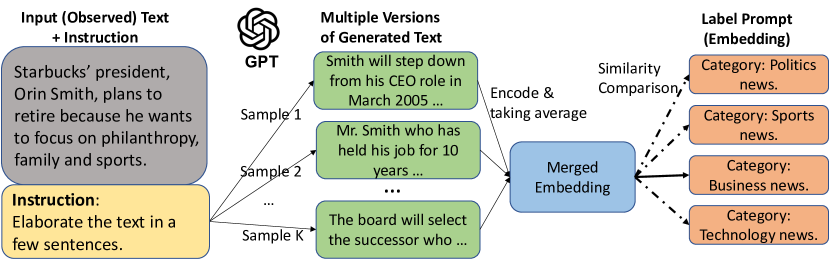
Figure 1: Input Text Augmentation using GPT Models: The input text and an instruction are fed into the GPT model to generate multiple pieces of elaborated texts, each of which is concatenated to the original input to obtain an augmented text. The embeddings of the augmented texts are then averaged to obtain a merged embedding, which is used for label prediction in the self-training process.

We first introduce the sentence encoder classifier as our basic design choice, and then focus on the novel components in our framework in the follow-up sections.

2.1 Zero-shot Text Classification as Sentence Alignment

The task of zero-shot text classification involves predicting the most relevant labels for a given document without requiring any labeled training data. Given a set of $N$ unlabeled documents $X=\{x_{1},x_{2},\cdots,x_{N}\}$ and a set of $L$ category descriptions $C=\{c_{1},c_{2},\cdots,c_{L}\}$, the goal is to learn a scoring function $g(x,c)$ that takes document $x$ and label description $c$ as input and produces a similarity score as the measure of how well the document and the label match to each other. In the rest of the paper, we assume each input text as a sentence for convenience, which can be easily generalized to a multi-sentence passage or document without jeopardizing the key concepts.

In the absence of labeled training data, the task of assigning labels to text can be formulated as a sentence alignment problem. This involves encoding both the input sentence and the label descriptions using a pre-trained sentence encoder like SimCSE Gao et al. (2021). The alignment scores between the sentence and labels embeddings are then used to predict related labels. This approach is particularly suitable for zero-shot classification as it relies on the semantic matching between textual instances and label descriptions in the embedding space, instead of relying on the availability of labeled training data.

However, as label descriptions are often just a few words instead of long sentences, they may not provide enough context for a pre-trained encoder to grasp the semantic meaning of the labels. To address this issue, prompt-based approaches Schick and Schütze (2020a) convert label names into natural language sentences, namely label prompts. For example, the label “sports" can be converted to “This is an article about sports." Following this, we denote by $p(\cdot)$ as a function that converts label name $c$ into a prompt by placing the label description into a predefined template. We design $T$ templates for each dataset and the label prompt embedding for category $c$ is defined as:

$${\bm{e}}_{c}=\frac{1}{T}\sum_{i=1}^{T}f_{\theta}\left(p^{i}(c)\right)$$ (1)

where $f_{\theta}(\cdot)$ is the sentence encoder parameterized by $\theta$. The scoring function can be implemented as:

$$g(x,c)=\operatorname{sim}\left(f_{\theta}(x),{\bm{e}}_{c}\right)$$ (2)

where $\mathrm{sim}(\cdot,\cdot)$ is a similarity function such as dot product or cosine similarity.

Given a input text at inference time, the predicted label is the one with the highest similarity score:

$$\hat{y}=\operatorname*{arg\,max}_{j}g\left(x,c_{j}\right)$$ (3)

2.2 Input Text Augmentation

In this section, we propose a way to enhance the semantic embedding of the original input text with multiple GPT-generated pieces of texts, as shown in figure 1. When the input text is relatively short, such as consisting of only one or a few sentences, the alignment-based matching to relevant labels may not be sufficiently effective. A natural remedy is to elaborate the input with a pre-trained GPT model to generate multiple pieces of texts. Specifically, we use a simple human instruction, "Elaborate the text with a few sentences," to guide the instruction-tuned GPT model, such as Alpaca-7B Taori et al. (2023), in generating probable expansions and continuations of the text. Our system treats the concatenation of the input text and each GPT-generated piece as one augmentation, and then takes the average of the embeddings of multiple augmentations as the merged embedding of the augmented input. Intuitively, such an augmentation should enhance the semantic matching among input text and relevant labels if the meaning of the input is underrepresented (too short) and if the generative model is highly effective in generating relevant pieces for the given input. The first assumption is often true in realist textual data, and the second condition is well-met by large pre-trained GPT models.

Formally, the input text $x\sim P(x)$ can be viewed as randomly sampled from an underlying distribution, and the augmented texts can be viewed as the different variants sampled from the conditional probability distribution induced by the GPT model, denoted as $x^{\text{aug}}\sim P_{g}(\cdot|x)$. We obtain the augmented text embedding by averaging the embeddings of the multiple versions of the augmented text:

$$\frac{1}{K}\sum_{i=1}^{K}f_{\theta}(x\oplus x_{i}^{\text{aug}}),$$ (4)

where $\oplus$ is the concatenation operator for text and $x_{i}^{\text{aug}}$ is the $i$-th sample from $P_{g}(\cdot|x)$. Our augmented texts provide different views of the input text, and the mean of the embedding provides an ensemble of induced features. We then use the augmented text embedding for pseudo-label prediction. If GPT is available at test time, we can use this method for inference as well.

2.3 Self-Training with Contrastive Learning

We employ a contrastive self-training process to enhance a pre-trained classifier’s generalization capability to iteratively augmented training data. Specifically, it is an iterative process where the pre-trained model is used to classify unlabeled data, and the newly classified data with high confidence is then used to further train the model. When the labels are noisy, previous studies have suggested using soft labeling Xie et al. (2016); Meng et al. (2020) or label smoothing Müller et al. (2019) to prevent the model from becoming overly confident. In this work, we propose a loss function with soft labeling that connects contrastive learning and entropy regularization Grandvalet and Bengio (2004).

We denote $f_{\theta}(x)$ as our sentence encoder model. Given a input text $x$, the distribution over labels is:

$$P(\hat{y}_{i}|x;\theta)=\frac{\exp(\operatorname{sim}(f_{\theta}(x),f_{\theta}(p_{i})))}{\sum_{c\in C}\exp(\operatorname{sim}(f_{\theta}(x),f_{\theta}(p_{c})))}$$ (5)

Here, $p_{i}$ is a shorthand notation for $p(c_{i})$, a randomly sampled label prompt for label $c_{i}$. The target distribution is derived as:

$$Q(\hat{y}_{i}|x;\theta)=\frac{\exp(\operatorname{sim}(f_{\theta}(x),f_{\theta}(p_{i}))/\tau)}{\sum_{c\in C}\exp(\operatorname{sim}(f_{\theta}(x),f_{\theta}(p_{c}))/\tau)}$$ (6)

where $\tau\leq 1$ is the temperature. A lower temperature implies a sharper distribution and thus greater confidence in the predicted label. We drop the notation of $\theta$ for convenience. The contrastive text to label ($t2l$) objective function is defined as:

$$\mathcal{L}_{t2l}=-\sum_{i=1}^{N}\sum_{j=1}^{L}Q(\hat{y}_{j}|x_{i})\log P(\hat{y}_{j}|x_{i})$$ (7)

When $\tau\rightarrow 0$, $Q(\hat{y}|x)$ becomes categorical distribution and the loss reduces to the supervised contrastive learning loss with pseudo label $\hat{y}_{c}$ as the target:

$$\mathcal{L}_{t2l}^{\tau\rightarrow 0}=-\sum_{i=1}^{N}\log P(\hat{y}_{c}|x_{i})$$ (8)

It encourages the model to predict label $c_{i}$ given $x$ with more confident. On the other hand, when $\tau=1$, the loss reduces to a minimization of conditional entropy function $H$:

$$\mathcal{L}_{t2l}^{\tau=1}=H\left(C\mid X\right)$$ (9)

$$=-\sum_{i=1}^{N}\sum_{j=1}^{L}P(\hat{y}_{j}|x_{i})\log P(\hat{y}_{j}|x_{i})$$ (10)

We show a theorem such that minimizing the loss function equation 7 can achieve similar effects Entropy Regularization Grandvalet and Bengio (2006, 2004), which is a means to enforce the cluster assumption such that the decision boundary should lie in low-density regions to improve generalization performance Chapelle and Zien (2005).

Theorem 1.

Consider a binary classification problem with linearly separable labeled examples. When $0<\tau<1$, optimizing equation 7 with gradient descend will enforce the larger margin between classes and achieves max margin classifier under certain constraint.

We place our formal theorems and proofs in Appendix section A. In our experiment, we set $\tau=0.1$ to balance supervised classification and low density separation between classes.

While self-learning was effective in improving the performance of our model, it is not without its limitations. One potential issue is overfitting to the pseudo label, which is prone to error. Additionally, self-learning requires a large amount of unlabeled data, which may not always be available. In the following section, we propose conditional augmentation methods with generative model in the training loop to make self-learning more robust.

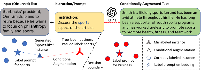
Figure 2: Augmented Text Generation Conditioned on Pseudo Labels: When a pseudo label is incorrect, it can mislead the training process and decrease classification performance. We generate augmented text conditioned on the pseudo label, aiming to make the generated text closer to the majoriry members in the category of the pseudo label. This approach aims to improve the quality of the generated instances for self-training.

2.4 Augmentation Conditioned on Prediction

The loss function of equation 7 can effectively enhance the separability of class instances by enforcing the decision boundary to lie in low density regions of the embedding space. In each self-training iteration, when the sampled instances are labeled with relatively lower confidence, which lie near the decision boundary, the contrastive loss pushes the instances closer to the pseudo label prompt embedding. However, self-training can lead to an undesirable bias in the classifier when instances are mislabeled. To address this issue, we propose a novel approach to the generation of labeled data for self-training. That is, we use GPT to generate labeled training pairs by augmenting each input text conditioned on the system-predicted (pseudo) labels, as shown in figure 2. For example, if a business news article discussing the retirement of Starbucks’ president is misclassified with the label of "sports", optimizing the model with this mislabeled training instance will make the decision boundaries between business articles less separable from sport articles. To alleviate such an undesirable effect, we use GPT to augment the input text conditioned on the sport category, resulting in a text closer to the typical ones in the sport category instead of the original one which lies closely to the decision boundary between "sports" and "businesses". In other words, by using GPT to generate augmented texts conditioned on pseudo labels, we aim to enhance the system-produced training pair with better separation of class labels in the embedding space.

Based on the aforementioned intuition, we propose an approach called instruction-based conditional generation to generate augmented text conditioned on the pseudo label. In this approach, we incorporate the predicted label information into the instructions provided to the model. For instance, we can use the instruction “Discuss the sports aspects of the article" to guide the model in generating text that is more relevant to the sports category.

Additionally, we propose two loss functions to enhance the self-training algorithm with the augmented text as follows.

Require: Unlabeled texts $X$, label descriptions $C$, pre-trained GPT model $g(\cdot)$.

Initialization: Classifier $f_{\theta}(\cdot)$ initialized with pre-trained sentence encoder. Empty dictionary $\operatorname{GenDict}$ to cache conditional generated text.

Input augmentation: For each observed text, generate $K$ samples of augmented text from $P_{g}(\cdot|x)$.

for $t:1\rightarrow T$ self-training iterations do

       Use $f_{\theta}(\cdot)$ to generate pseudo-labels $\hat{y}$ (eq.3) and soft-labels $Q$ (eq.6) for texts with input augmentation. Sample a balanced subset of pseudo-labeled training pairs of size $S_{t}$ according to prediction confidence;

       for each training sample $(x,\hat{y})$ do

             if key $(x,\hat{y})\in\operatorname{GenDict}$ then

                   Fetch generated texts from $\operatorname{GenDict}$ $\triangleright$ Use cached generated text

            else

                   Generate $M$ samples from $P_{g}(\cdot|x,\hat{y})$ $\triangleright$ Conditional augmentation;

                   Add generated texts to $\operatorname{GenDict}$ $\triangleright$ Cached generated text;

                  

            

      Use sampled training pairs and the conditionally generated text to update the parameters $\theta$ of $f_{\theta}(\cdot)$ with the objective function $\mathcal{L}=\mathcal{L}_{g2l}+\mathcal{L}_{t2g}$.

Algorithm 1 Self-training with GPT model assisted in the loop

2.4.1 Contrastive Learning for Conditionally Augmented Text and Label Prompt

To alleviate the problem of erroneous label assignment, we use the conditional augmented text ($x^{\text{c\_aug}}\sim P_{g}(\cdot|x,\hat{y})$) and the pseudo label prompt as positive pairs.

$$\mathcal{L}_{g2l}=-\sum_{i=1}^{N}\sum_{j=1}^{L}Q(\hat{y}_{j}|x_{i}^{\text{c\_aug}})\log P(\hat{y}_{j}|x_{i}^{\text{c\_aug}})$$ (11)

2.4.2 Contrastive Learning for Observed Text and Augmented Text

For document representation, the contrastive pairs are usually created by sampling spans of document Izacard et al. (2022). In our case, the generative model naturally creates different views of data and we use the contrastive loss between observed text and generated text for optimization:

$$\begin{split}&\mathcal{L}_{t2g}=\sum_{i\in\mathit{I}}\frac{-1}{|A(i)|}\\ &\sum_{x^{\text{aug}}\in A(i)}\log{\frac{\exp({sim(f_{\theta}(x_{i}),f_{\theta}(x^{\text{aug}}))})}{\sum_{j\in\mathit{I}}\exp(sim(f_{\theta}(x_{i}),f_{\theta}(x_{j})))}}.\end{split}$$ (12)

where $\mathit{I}$ is a training batch and $A(i)$ denotes the set of augmented texts belonging to the same pseudo class of input $x_{i}$.

Algorithm 1 shows the self-training of GenCo with generative model assisting in the self-training loop. During training, we found that a balanced sampling that keeps the same number ($S_{t}$ for iteration $t$) of training for each category is important for the stability of self-training. Additionally, we use a dictionary to cache the conditional generated text to avoid repeated generation.

3 Experiments

3.1 Datasets and Experimental Settings

Dataset	Classification Type	#Classes	#Train	#Test	Avg Length
AG News	News Topic	4	120,000	7,600	38
DBPedia	Wikipedia Topic	14	560,000	70,000	50
Yahoo Answers	Quetion Answering	10	1,400,000	60,000	70
Amazon	Product Review Sentiment	2	3,600,000	400,000	78

Table 1: Statistics of datasets for multi-class text classification.

Label Prompt

(1)Category: [label]. (2)It is about [label].

Instruction-based (Conditional) Augmentation

Below is an instruction that describes a task, paired with an input that provides further context. Write a response that appropriately completes the request. ### Instruction: Elaborate the text in a few sentences. (Discuss the [pseudo label] aspects of the article.) ### Input: $[$text$]$ ### Response:

Table 2: The designed prompts for enhanced label description and conditional augmentation based on pseudo label.

We conduct experiments on $4$ benchmark text classification datasets: AG News, DBpedia, Yahoo Answers and Amazon, with the statistics shown in table 1. In the experiments, we initialize our sentence encoder with supervised SimCSE Roberta-base model Gao et al. (2021). The designed prompts for enhanced label description is illustrated in table 2. For the generative model, we use the Alpaca-7B Taori et al. (2023) model, which is an open source GPT model fine-tuned with human instructions Touvron et al. (2023). The prompts for instruction-based augmentation (table 2) is the same as the one used in the Alpaca model fine-tuning. For the generation parameters, we used $temperature$=0.8, $top\_p$=0.95, and sample $K$=5 augmented texts for each instance with $min\_length=64$ and $max\_length=128$. For the self-training of sentence encoder model, we used $batch\_size$=$3*|C|$ ($|C|$ is the number of categories), $lr$=1e-5, the max length is $128$ for AG News and DBPedia and $192$ for Yahoo Answers and Amazon. All the experiments are performed on NVIDIA RTX A6000 gpus.

3.2 Baseline Methods

• PET Schick and Schütze (2020b) method formulates zero-shot text classification as a cloze test tasks, where a pretrained BERT Devlin et al. (2018) model is used to predict the output label(s) by completing a prompt such as “This article is about _", which is concatenated right after an input document.

• iPET Schick and Schütze (2020b) uses a self-training algorithm to improve from the PET model, where multiple generations of models are trained by gradually increasing the number of training instances labeled by a model trained in the previous generation.

• LOTClass Meng et al. (2020) first applies the BERT model to extract keywords related to the label names from unlabeled texts and then assigns pseudo labels for texts based on the extracted keywords. LOTClass also applies a self-training algorithm to further improve the classification performance.

• Other Baselines We include prompt-based GPT model, a sentence-encoder based model without any self-training and a self-training baseline without any text augmentation. Additionally, a supervised learning baseline is included for reference.

3.3 Main Results

ID	Self-train	Methods	AG News	DBpedia	Yahoo Answers	Amazon
1	–	Supervised	94.2	99.3	77.3	97.1
2	No	PET	79.4	75.2	56.4	87.1
3	Yes	iPET	86.0	85.2	68.2	95.2
4	Yes	LOTClass	86.4	91.1	–	91.6
5	No	Sentence-enc (SimCSE)	74.5	73.8	55.6	88.8
6	No	GPT (Alpaca-7B)	71.2	65.5	52.1	87.2
7	–	Supervised-downsample*	93.8	98.7	76.5	97.0
8	Yes	GenCo-instruction*	89.2	98.3	68.7	95.4

Table 3: Comparison of classification methods on benchmark datasets. The test accuracy of best performing zero-shot method is highlighted in bold phase. Row 7-8 (with *) use a downsampled dataset with 4k (3.4%), 11.2k (2%), 15k ($<$1%), 20k ($<$1%) unlabeled training instances respectively.

In table 3, we present a comparison of the test accuracy of our model with other baselines on four benchmark classification datasets. Due to the large number of text instances, it was not feasible to perform augmentation using the entire dataset. Instead, our model was trained on a downsampled dataset, with uniform sampling resulting in less than 2% of the original data used (rows 7-8). Despite the reduced size of the dataset, we observed that our proposed model GenCo still outperforms the other zero-shot baseline methods and is close to supervise learning settings (row 1 and 7).

Compared with SOTA Methods Both LOTClass and iPET use a self-training algorithm for zero-shot classification, but our adaptation of GPT model can better enhance the self-training performance. Specifically, LOTClass uses a BERT model to extract keywords for each category, and employs lexical matching between input text and the keywords to assign pseudo labels. While the keywords can be considered as an augmentation, it is less expressive than using a GPT model to generate coherent human language as augmentation. Our proposed method uses a sentence encoder with more expressive neural features, making it more effective than using lexical-based features to assign pseudo labels. The iPET model requires training multiple models and ensembling about 15 of them, which is memory extensive. While ensembling can stabilize self-training by reducing variance, it does not introduce new information about the input text. Our approach uses a generative model to augment text data during self-training, leading to improved performance and a more memory efficient alternative.

Comparison with GPT: While GPT (row 6) has demonstrated strong zero-shot performance in various tasks, it underperforms compared to our sentence-encoder classifier baseline (row 5), which is fine-tuned using contrastive learning on the Natural Language Inference dataset Gao et al. (2021), in the context of text classification. Classification involves comparing instances, such as an article being more likely to belong to the “sports" category when compared to articles in the “business" category. Contrastive learning leverages this comparison and our contrastive self-training further improves it.

ID	Self-train	Methods	AG News	DBpedia	Yahoo Answers	Amazon
# unlabeled train				4k (3.4%)	11.2k (2%)	15k ($<$ 1%)	20k ($<$ 1%)
# unlabeled test			7.6k	28k	20k	20k
1	No	Sentence-enc	75.6	73.4	55.5	89.6
2	No	Sentence-enc $+$ IA	78.2	74.7	57.4	90.2
3	Yes	Self-train	83.3	96.3	62.5	91.1
4	Yes	Self-train $+$ IA	83.9	96.8	64.3	91.3
5	Yes	Self-train $+$ TA	86.9	97.0	66.1	94.4
6	Yes	Self-train $+$ TA $+$ IA	87.1	97.1	67.2	94.6
7	Yes	GenCo	89.2	98.4	68.6	95.3
8	Yes	GenCo $+$ IA	89.7	98.5	70.2	95.4

Table 4: Results of ablation test for our proposed method, showing the effect of specific components on the performance metric. “TA" represents input augmentation added during training, while “IA" represents input augmentation added during inference.

In table 4, we present the impact of inference time augmentation (assuming GPT is available at test time) and self-training on the performance metric. To test inference time augmentation, we performed experiments on a downsampling of both training and testing instances.

Inference Time Augmentation: Our results show that inference time augmentation (rows with "IA") leads to a performance gain of $1$-$2\%$, with a more substantial improvement observed for AG News and Yahoo Answers. This may be attributed to the fact that AG News has an average text length of only $38$ words, and the Yahoo Answers dataset includes many answers with only one phrase. Inference time augmentation effectively enhances the quality of shorter text inputs.

Self-Training: Our experiments demonstrate that self-training improves the performance on all datasets, even in the absence of augmented data (rows 3-4). The DBpedia dataset exhibits an improvement of over 20%. Theoretically, self-training enhances the separation of text, thereby making the decision boundary lie in the low-density area, which is critical for classification. Our generative-driven approaches, with and without conditioning on pseudo label, both lead to improved performance. However, the conditional augmentation approach is more effective due to its ability to stabilize self-training.

3.4 Analysis of Input Augmentation

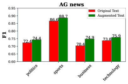
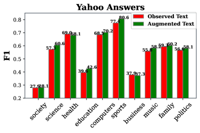
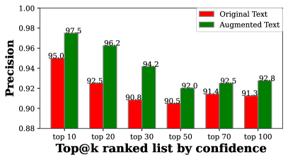
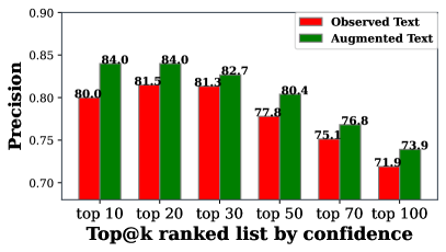
Figure 3: Per class F1 (upper) and ranking-based precision (lower) for classification performance with input augmentation.

In this evaluation, we investigate the effectiveness of input augmentation for zero-shot inference without training. We evaluate the performance of our model on two datasets, namely AG News and Yahoo Answers, using two evaluation metrics: per class F1 metric and ranking-based precision metric according to prediction confidence. The per class F1 metric provides an insight into how well the model performs on each individual class by balancing precision and recall. In the upper part of figure 3, our findings indicate that using GPT augmented data leads to improved performance across all categories for AG News and in eight out of ten classes for Yahoo Answers.

In the lower part of figure 3, we employ a ranking-based precision metric to assess the quality of the most confident cases. Our results demonstrate that using augmented data yields better precision for the most confident cases. Notably, our study on the Yahoo Answers dataset indicates that the predictions are better calibrated with the use of augmented data, implying that highly confident samples exhibit better precision. Conversely, such a trend was not observed in unaugmented data, where the top 30 had higher accuracy than the top 10. Better calibration justifies the sampling from the most confident pools for self-training, making it a more reliable method for improving model performance.

3.5 Analysis of Conditional Augmentation

Observed Text Starbucks Corp’s president and chief executive, Orin Smith, said Tuesday he plans to retire early next year because he wants to slow down and focus on philanthropy, family and sports. Politics The announcement of Orin Smith’s retirement is likely to have political implications for Starbucks Corporation… His replacement will have big shoes to fill, and the decision could have long-term effects on the company’s policies and direction. Sports …Sports have always been a major part of Smith’s life, as he was a college athlete and later went on to become the CEO of Starbucks. It is clear that sports have had a major influence on his life and he wants to make time for them in his retirement. Business Starbucks Corp has seen great success under the leadership of Orin Smith, with the company’s stock price more than tripling since he became CEO in 2005. This success has allowed him to retire early and … Technology Orin Smith’s plan to retire early next year is an example of how technology has changed the way we work and live. By utilizing technology, Smith is able to take advantage of the increasingly popular trend of “work-life balance" …

Table 5: Examples of generated text conditioned on pseudo labels in the left column.

In table 5, we present generated texts conditioned on an sample in AG News dataset and the pseudo labels. Each example is a cherry-picked sample out of five random samples. The generated text expands on a specific aspect regarding the label while retaining the original meaning of the observed text.

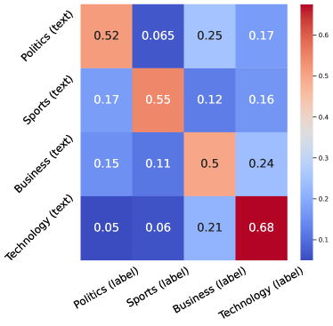
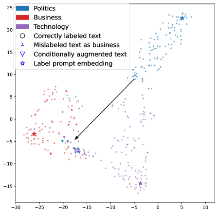
Figure 4: The left figure shows a heatmap of the probability that a conditionally generated text falls into the corresponding pseudo label category. The right figure shows the distribution of the generated text plotted using T-SNE (sports category is out of scope).

The left figure in figure 4 shows a heatmap of the probability that a conditionally generated text falls into the corresponding pseudo label category. The highest probability occurs along the diagonal, indicating that the conditionally generated data has a closer meaning to the pseudo label. The right figure in figure 4 shows the distribution of the generated text plotted using T-SNE. The embeddings were obtained by our sentence encoder trained on the $100$-th iteration. We selected two instances that were misclassified as business and located close to the decision boundary. The augmented text, conditioned on the business category, was found to be closer to the label prompt embedding of the business category. This demonstrates the effectiveness of our method to generate less confusing training pairs away from the decision boundary.

4 Related Work

4.1 Knowledge Distillation from GPT

To leverage the language modeling power of large model, previous worksYoo et al. (2021); Ye et al. (2022); Meng et al. (2022) use GPT to generate text and label pairs to train a classifier for downstream tasks. However, generating training data from scratch can lead to low-quality data with unrelated or ambiguous generated text Gao et al. (2022). Our approach also generates text data, but it is grounded in the context of the corpus of interest, and further enhances the quality and semantic diversity of the generated text. This approach provides a practical alternative to generation-based methods for zero-shot text classification.

4.2 Sentence Encoder and Contrastive Learning

Sentence encoders Gao et al. (2021) model the alignment of sentences by their similarity in the embedding space, which can be adopted to the zero-shot text classification task Hong et al. (2022); Shi et al. (2022). Sentence encoders are typically trained with contrastive learning, which optimizes representations by pulling inputs with similar semantics closer in the embedding space and pushing inputs with different semantics further apart. Recent approaches Izacard et al. (2022) sample positive pairs from spans of the same document and negative pairs from different documents in the training batch. Our model applies GPT to generate training pairs for contrastive learning.

4.3 Self-training Methods

Self-training methods Van Engelen and Hoos (2020) have been proposed as a semi-supervised approach to improve a classifier from unlabeled datasets, where predictions on unlabeled data are used to fine-tune the classifier Lee et al. (2013). To improve the pseudo label quality, previous work Gera et al. (2022) use a small set of instances with the most confident prediction for self-training. LOTClass Meng et al. (2020) improves the quality of pseudo label by an expansion of label vocabulary using BERT and iPET Schick and Schütze (2020b) ensembles multiple version of model at different stage of training. Our work improves self-training by generating augmented text with GPT in the training loop.

4.4 Authors’ Considerations and Limitations

The main goal of our paper is to promote the usage of pre-trained GPT model (Alpaca-7B) to assist in training of a smaller model (Roberta-SimCSE) on zero-shot classification tasks. We are aware that there are rooms more experiments with self-training algorithms, such as how the temperature of our loss function can affect the training stability. Currently, we only use that as a theoretical motivation of leveraging decision boundaries between classes, but tuning the temperature will be additional work to do.

Another part is data efficiency. We have shown that using GPT generated data can alleviate the data hungry issue in deep learning models for text classification, but more comprehensive study can be done by applying the baseline models on the down-sampled dataset and analyzing the performance in those scenarios.

Finally, we realize that more tricks and engineering designs are employed in our experiments and we have released our code on github for reference.

5 Conclusion

In conclusion, our proposed approach, GenCo, effectively addresses the difficulties and limitations of using pretrained large GPT models directly for zero-shot text classification. By leveraging the generative power of GPT models in a self-training loop of a smaller, sentence encoder classifier with contrastive learning, GenCo outperform state-of-the-art methods on four benchmark datasets. Our approach is particularly effective when limited in-domain text data are available. The success of our approach highlights the potential benefits of incorporating the generative power of GPT models into iterative self-training processes for smaller zero-shot classifiers. We hope that our work will inspire further research in this direction, ultimately leading to more efficient and effective NLP models.

Appendix A Proof of Theorems

Theorem 2.

Consider a binary classification problem with linearly separable labeled examples, when $0<\tau<1$, optimizing $\mathcal{L}_{t2l}=-\sum_{i=1}^{N}\sum_{j=1}^{L}Q(\hat{y}_{j}|x_{i})\log P(\hat{y}_{j}|x_{i})$ with gradient descend will enforce the larger margin between classes.

Proof.

We use dot product $\langle\cdot,\cdot\rangle$ as implementation of similarity function. Let the embedding of instance $i$ be ${\bm{x}}_{i}=f_{\theta}(x_{i})$ and the embedding of label prompt $j$ be ${\bm{e}}_{c}=f_{\theta}(p_{c}),c\in\{1,2\}$ for binary classification. Then,

$$P(\hat{y}_{1}|x_{i};\theta) =\frac{\exp(\langle{\bm{x}}_{i},{\bm{e}}_{1}\rangle)}{\exp(\langle{\bm{x}}_{i},{\bm{e}}_{1}\rangle)+\exp(\langle{\bm{x}}_{i},{\bm{e}}_{2}\rangle)}=\frac{1}{1+\exp(-\langle{\bm{x}}_{i},{\bm{e}}_{1}-{\bm{e}}_{2}\rangle)}$$ (13)

$$P(\hat{y}_{1}|x_{i};\theta) =1-P(\hat{y}_{0}|x_{i};\theta)$$ (14)

Notation-wise, define $d_{i}=\langle{\bm{x}}_{i},{\bm{e}}_{1}-{\bm{e}}_{2}\rangle$, then

$$P(\hat{y}_{1}|x_{i};\theta) =\frac{1}{1+e^{-d_{i}}}$$ (16)

$$P(\hat{y}_{1}|x_{i};\theta) =1-\frac{1}{1+e^{-d_{i}}}$$ (17)

In binary classification, the margin is simply

$$\text{margin}=\begin{cases}d_{i}&x_{i}\text{ is class 1}\\ -d_{i}&x_{i}\text{ is class 2}\end{cases}$$

For soft-label distribution $Q$,

$$Q(\hat{y}_{1}|x_{i};\theta) =\frac{1}{1+e^{-d_{i}/\tau}}$$ (19)

$$Q(\hat{y}_{1}|x_{i};\theta) =1-\frac{1}{1+e^{-d_{i}/\tau}}$$ (20)

Then $\mathcal{L}_{t2l}$ is derived as

$$\mathcal{L}_{t2l}=\sum_{i=1}^{N}\log(1+e^{-d_{i}})+\frac{d_{i}e^{-d_{i}/\tau}}{1+e^{-d_{i}/\tau}}$$ (22)

Calculate the derivative of $\mathcal{L}_{t2l}$ w.r.t $d_{i}$,

$$\frac{\partial\mathcal{L}_{t2l}}{\partial d_{i}}=\frac{-d_{i}e^{-d_{i}/\tau}}{t(e^{-d_{i}/\tau}+1)^{2}}+\frac{e^{-d_{i}/\tau}-e^{-d_{i}}}{(e^{-d_{i}/\tau}+1)(e^{-d_{i}}+1)}$$ (23)

For the first part of equation 23, the sign depends on $-d_{i}$. For the second part, the sign depends on $e^{-d_{i}/\tau}-e^{-d_{i}}$. When $0<\tau<1$,

$$\begin{cases}e^{-d_{i}/\tau}-e^{-d_{i}}<0&\text{when }d_{i}>0\\ e^{-d_{i}/\tau}-e^{-d_{i}}>0&\text{when }d_{i}<0\end{cases}$$

Therefore,

$$\begin{cases}\frac{\partial\mathcal{L}_{t2l}}{\partial d_{i}}<0&\text{when }d_{i}>0\\ \frac{\partial\mathcal{L}_{t2l}}{\partial d_{i}}>0&\text{when }d_{i}<0\end{cases}$$ (24)

One step of gradient descend optimizes $d$ by $d_{i}^{\prime}=d_{i}-\eta\frac{\partial\mathcal{L}_{t2l}}{\partial d_{i}}$. From equation 24, we get the conclusion that $|d_{i}^{\prime}|>|d_{i}|$. In other words, the margin becomes larger after optimization, which finishes the proof. ∎

Theorem 3.

Under the setting in Theorem 2, let $m_{i}$ be the margin of instance $i$ and consider the constraint $m_{i}\leq B$ for all $i$, the classifier converges to a max margin classifier, as the bound $B$ goes to infinity.

Proof.

Using the definition from Theorem 2,

$$\mathcal{L}_{t2l}=\sum_{i=1}^{N}\log(1+e^{-d_{i}})+\frac{d_{i}e^{-d_{i}/\tau}}{1+e^{-d_{i}/\tau}}$$ (25)

The margin $m_{i}$ for instance $i$ can be written as $m_{i}=\begin{cases}d_{i}&x_{i}\text{ is class 1}\\ -d_{i}&x_{i}\text{ is class 2}\end{cases}$.

The equation 25 can be written as

$$\mathcal{L}_{t2l}=\sum_{y_{i}=0}\log(1+e^{-m_{i}})+\frac{m_{i}e^{-m_{i}/\tau}}{1+e^{-m_{i}/\tau}}+\sum_{y_{j}=1}\log(1+e^{m_{j}})-\frac{m_{j}e^{m_{j}/\tau}}{1+e^{m_{j}/\tau}}$$ (26)

Let $m^{*}=\min(m_{i})$ be the minimal margin, let $N_{1}$ and $N_{2}$ be the number of instances in class 1 and class 2 respectively which reaches the minimal margin. From the gradient analysis in equation 24, the examples with $m_{i}>m^{*}$ has loss lower bounded by that with minimal margin. Then

$$\begin{split}\mathcal{L}_{t2l}&=N_{1}(\log(1+e^{-m^{*}})+\frac{m^{*}e^{-m^{*}/\tau}}{1+e^{-m^{*}/\tau}})+N_{2}(\log(1+e^{m^{*}})-\frac{m^{*}e^{m^{*}/\tau}}{1+e^{m^{*}/\tau}})\\ &+O(\log(1+e^{-m^{*}})+\frac{m^{*}e^{-m^{*}/\tau}}{1+e^{-m^{*}/\tau}})+O(\log(1+e^{m^{*}})-\frac{m^{*}e^{m^{*}/\tau}}{1+e^{m^{*}/\tau}})\end{split}$$ (27)

When $B$ approaches $\infty$, for $N_{1}$ part in equation 27,

$$\log(1+e^{-m^{*}})+\frac{m^{*}e^{-m^{*}/\tau}}{1+e^{-m^{*}/\tau}}\sim e^{-m^{*}}+m^{*}e^{-m^{*}/\tau}$$ (28)

When $m\rightarrow B$, $\lim_{m\rightarrow B}e^{-m^{*}}\rightarrow 0$, and $\lim_{m\rightarrow B}m^{*}e^{-m^{*}/\tau}=\lim_{m\rightarrow B}\frac{1}{1/\tau e^{m^{*}/\tau}}=0$ by L’Hopital’s rule.

For $N_{2}$ part in equation 27,

$$\log(1+e^{m^{*}})-\frac{m^{*}e^{m^{*}/\tau}}{1+e^{m^{*}/\tau}}\sim\log(1+e^{m^{*}})-m^{*}$$ (29)

When $m\rightarrow B$, $\lim_{m\rightarrow B}\log(1+e^{m^{*}})-m^{*}=\lim_{m\rightarrow B}\log(1+\frac{1}{e^{m^{*}}})=0$.

Therefore, the loss is minimized when the minimal margin is maximized and thus the classifier converges to a max margin classifier when $B$ goes to infinity. ∎

References

- Brown et al. (2020) Tom B Brown, Benjamin Mann, Nick Ryder, Melanie Subbiah, Jared Kaplan, Prafulla Dhariwal, Arvind Neelakantan, Pranav Shyam, Girish Sastry, Amanda Askell, et al. 2020. Language models are few-shot learners. arXiv preprint arXiv:2005.14165.
- Chapelle and Zien (2005) Olivier Chapelle and Alexander Zien. 2005. Semi-supervised classification by low density separation. In International workshop on artificial intelligence and statistics, pages 57–64. PMLR.
- Devlin et al. (2018) Jacob Devlin, Ming-Wei Chang, Kenton Lee, and Kristina Toutanova. 2018. Bert: Pre-training of deep bidirectional transformers for language understanding. arXiv preprint arXiv:1810.04805.
- Gao et al. (2022) Jiahui Gao, Renjie Pi, Yong Lin, Hang Xu, Jiacheng Ye, Zhiyong Wu, Xiaodan Liang, Zhenguo Li, and Lingpeng Kong. 2022. Zerogen: Self-guided high-quality data generation in efficient zero-shot learning. arXiv preprint arXiv:2205.12679.
- Gao et al. (2021) Tianyu Gao, Xingcheng Yao, and Danqi Chen. 2021. Simcse: Simple contrastive learning of sentence embeddings. arXiv preprint arXiv:2104.08821.
- Gera et al. (2022) Ariel Gera, Alon Halfon, Eyal Shnarch, Yotam Perlitz, Liat Ein-Dor, and Noam Slonim. 2022. Zero-shot text classification with self-training. arXiv preprint arXiv:2210.17541.
- Grandvalet and Bengio (2004) Yves Grandvalet and Yoshua Bengio. 2004. Semi-supervised learning by entropy minimization. Advances in neural information processing systems, 17.
- Grandvalet and Bengio (2006) Yves Grandvalet and Yoshua Bengio. 2006. Entropy regularization.
- Hong et al. (2022) Jimin Hong, Jungsoo Park, Daeyoung Kim, Seongjae Choi, Bokyung Son, and Jaewook Kang. 2022. Tess: Zero-shot classification via textual similarity comparison with prompting using sentence encoder. arXiv preprint arXiv:2212.10391.
- Izacard et al. (2022) Gautier Izacard, Mathilde Caron, Lucas Hosseini, Sebastian Riedel, Piotr Bojanowski, Armand Joulin, and Edouard Grave. 2022. Unsupervised dense information retrieval with contrastive learning.
- Lee et al. (2013) Dong-Hyun Lee et al. 2013. Pseudo-label: The simple and efficient semi-supervised learning method for deep neural networks. In Workshop on challenges in representation learning, ICML, volume 3, page 896.
- Meng et al. (2022) Yu Meng, Jiaxin Huang, Yu Zhang, and Jiawei Han. 2022. Generating training data with language models: Towards zero-shot language understanding. arXiv preprint arXiv:2202.04538.
- Meng et al. (2020) Yu Meng, Yunyi Zhang, Jiaxin Huang, Chenyan Xiong, Heng Ji, Chao Zhang, and Jiawei Han. 2020. Text classification using label names only: A language model self-training approach. arXiv preprint arXiv:2010.07245.
- Müller et al. (2019) Rafael Müller, Simon Kornblith, and Geoffrey E Hinton. 2019. When does label smoothing help? Advances in neural information processing systems, 32.
- Ouyang et al. (2022) Long Ouyang, Jeff Wu, Xu Jiang, Diogo Almeida, Carroll L Wainwright, Pamela Mishkin, Chong Zhang, Sandhini Agarwal, Katarina Slama, Alex Ray, et al. 2022. Training language models to follow instructions with human feedback. arXiv preprint arXiv:2203.02155.
- Schick and Schütze (2020a) Timo Schick and Hinrich Schütze. 2020a. Exploiting cloze questions for few shot text classification and natural language inference. arXiv preprint arXiv:2001.07676.
- Schick and Schütze (2020b) Timo Schick and Hinrich Schütze. 2020b. It’s not just size that matters: Small language models are also few-shot learners. arXiv preprint arXiv:2009.07118.
- Shi et al. (2022) Weijia Shi, Julian Michael, Suchin Gururangan, and Luke Zettlemoyer. 2022. Nearest neighbor zero-shot inference. arXiv preprint arXiv:2205.13792.
- Taori et al. (2023) Rohan Taori, Ishaan Gulrajani, Tianyi Zhang, Yann Dubois, Xuechen Li, Carlos Guestrin, Percy Liang, and Tatsunori B. Hashimoto. 2023. Stanford alpaca: An instruction-following llama model. https://github.com/tatsu-lab/stanford_alpaca.
- Touvron et al. (2023) Hugo Touvron, Thibaut Lavril, Gautier Izacard, Xavier Martinet, Marie-Anne Lachaux, Timothée Lacroix, Baptiste Rozière, Naman Goyal, Eric Hambro, Faisal Azhar, et al. 2023. Llama: Open and efficient foundation language models. arXiv preprint arXiv:2302.13971.
- Van Engelen and Hoos (2020) Jesper E Van Engelen and Holger H Hoos. 2020. A survey on semi-supervised learning. Machine learning, 109(2):373–440.
- Xie et al. (2016) Junyuan Xie, Ross Girshick, and Ali Farhadi. 2016. Unsupervised deep embedding for clustering analysis. In International conference on machine learning, pages 478–487. PMLR.
- Ye et al. (2022) Jiacheng Ye, Jiahui Gao, Qintong Li, Hang Xu, Jiangtao Feng, Zhiyong Wu, Tao Yu, and Lingpeng Kong. 2022. Zerogen: Efficient zero-shot learning via dataset generation. arXiv preprint arXiv:2202.07922.
- Yoo et al. (2021) Kang Min Yoo, Dongju Park, Jaewook Kang, Sang-Woo Lee, and Woomyeong Park. 2021. Gpt3mix: Leveraging large-scale language models for text augmentation. arXiv preprint arXiv:2104.08826.