Accurate and Efficient Event-based Semantic
Segmentation Using Adaptive Spiking
Encoder-Decoder Network

Abstract

Leveraging the low-power, event-driven computation and the inherent temporal dynamics, spiking neural networks (SNNs) are potentially ideal solutions for processing dynamic and asynchronous signals from event-based sensors. However, due to the challenges in training and the restrictions in architectural design, there are limited examples of competitive SNNs in the realm of event-based dense prediction when compared to artificial neural networks (ANNs). In this paper, we present an efficient spiking encoder-decoder network designed for large-scale event-based semantic segmentation tasks. This is achieved by optimizing the encoder using a hierarchical search method. To enhance learning from dynamic event streams, we harness the inherent adaptive threshold of spiking neurons to modulate network activation. Moreover, we introduce a dual-path Spiking Spatially-Adaptive Modulation (SSAM) block, specifically designed to enhance the representation of sparse events, thereby considerably improving network performance. Our proposed network achieves a 72.57% mean intersection over union (MIoU) on the DDD17 dataset and a 57.22% MIoU on the recently introduced, larger DSEC-Semantic dataset. This performance surpasses the current state-of-the-art ANNs by 4%, whilst consuming significantly less computational resources. To the best of our knowledge, this is the first study demonstrating SNNs outperforming ANNs in demanding event-based semantic segmentation tasks, thereby establishing the vast potential of SNNs in the field of event-based vision. Our source code will be made publicly accessible.

I Introduction

Evolved from biological neurons, spiking neuron models embody event-driven attributes and intrinsic temporal dynamics, leading to highly sparse and asynchronous activation in spiking neural networks (SNNs). Such characteristics establish SNNs as exceptional candidates for processing signals from retina-inspired event-based sensors [1, 2, 3]. These sensors generate spatial-temporal, highly asynchronous, and sparse data. The harmonious integration of event-based sensors and SNNs could potentially yield brain-inspired or neuromorphic sensory-processing systems with exceptionally low-power consumption [4, 5, 6, 7, 8].

Nevertheless, most leading research in event-based vision predominantly employs artificial neural networks (ANNs) with dense, frame-based computation [9, 10, 11, 12]. One major contributing factor to this is the relative complexity of gradient-based training of SNNs compared to ANNs. The membrane potential of a spiking neuron undergoes a continuous evolution, emitting a discrete spike whenever the potential surpasses a threshold. This discontinuity of spikes is incompatible with gradient-based backpropagation, which necessitates continuous differentiable variables. The surrogate gradient (SG) method alleviates this issue by substituting the original non-existent gradient with continuous smooth functions [13, 14, 15]. Utilizing this principle and implementing advanced learning algorithms, SNNs have recently achieved remarkable advancements in classification tasks on benchmark image and event-based datasets, reaching accuracy levels comparable to ANNs [16, 17, 18, 19, 20].

However, competitive demonstrations of SNNs in more complex vision tasks, such as dense prediction, remain scant. Network architecture represents a substantial obstacle. Sophisticated structures in ANNs, unlike those in classification tasks, often possess more variations and are not easily transferrable to SNNs. Crafting architectures for SNNs is limited by the intricacies inherent to their training and the additional costs of training time, leading to simple network structures with suboptimal performance [21, 22, 23]. Furthermore, the incompatibility of recent advanced techniques in deep learning, such as attention or normalization mechanisms [24, 25, 26], with multiplication-free inference (MFI) of spike-based computation hampers the incorporation of these potent operations in SNNs. This further detracts from the attractiveness of SNNs for large-scale vision tasks compared to ANNs.

In the present work, we develop SNNs for event-based semantic segmentation on two large-scale datasets. To the best of our knowledge, this is the first instance of SNNs outperforming sophisticated ANNs in these tasks. In summary, our contributions are as follows:

• We introduce and train an adaptive threshold for spiking neurons, demonstrating that this inherent mechanism enhances network performance by modulating spiking activation in response to highly dynamic input event streams.

• We design an efficient spiking encoder-decoder architecture for event-based semantic segmentation. The encoder is optimized via a spike-based hierarchical search at both the cell and layer levels.

• To bolster the representation of sparse events, we devise an MFI-compatible, dual-path Spiking Spatially-Adaptive Modulation (SSAM) block. This block significantly improves network performance and proves effective for both purely event-driven and combined frame-based inputs.

• Our network achieves a 72.57% MIoU on the DDD17 dataset, surpassing directly trained SNNs by 37% and ANNs by 4% in MIoU. On the high-resolution DSEC dataset, the same network delivers a 57.22% MIoU, exceeding the state-of-the-art ANN based on transfer learning by 4%. Evaluations of operation numbers and potential energy costs confirm that our networks are substantially more power-efficient than ANNs.

The remainder of this paper is structured as follows: Section II supplies the necessary background information, covering topics such as event-based semantic segmentation, SNNs for dense prediction, and adaptive threshold neurons. Section III commences with an overview of our spiking encoder-decoder network architecture, succeeded by an in-depth discussion on the spiking neuron with an adaptive threshold and Spiking Spatially-Adaptive Modulation. Section IV presents comprehensive experimental studies conducted on two datasets, DDD17 and DSEC-Semantic, inclusive of results from ablation studies, network sparsity analysis, random seed experiments, and gray-scale image testing. Finally, Section V summarizes our findings and offers concluding remarks.

II Background

This section provides the necessary background on various topics that underpin our research. We begin by discussing the concept of Event-based Semantic Segmentation (EbSS), highlighting its potential and current advancements. We then delve into the role of Spiking Neural Networks (SNNs) in dense prediction tasks, exploring recent developments and challenges in this area. Lastly, we focus on the Adaptive Threshold Neuron, its previous applications, and how we propose to leverage its potential in our work.

II-A Event-based Semantic Segmentation

Event-based cameras, characterized by superior temporal resolution (1us) and dynamic range (120dB) compared to frame-based cameras, are particularly suitable for high-speed edge platforms such as vehicles and drones. The field of event-based semantic segmentation (EbSS) is burgeoning with limited existing works, yet rapidly growing interest. EV-SegNet [11] first established a baseline for EbSS on the large-scale benchmark dataset, DDD17 [27]. Leveraging an Xception-based [28] encoder-decoder architecture, they devised an event data representation encapsulating both the event histogram and temporal distribution. More recent works involving transfer learning approaches [29, 12] harnessed knowledge gleaned from high-quality image datasets.

These works transferred semantic segmentation tasks from labeled image datasets to unlabeled events through unsupervised domain adaptation, thereby surpassing supervised methodologies. However, the knowledge distillation process they utilized can contribute to additional computation costs. The work in [22] was the first to explore the feasibility of directly training SNNs for EbSS on the DDD17 dataset, employing SNNs with handcrafted ANN architectures including DeepLab [30] and Fully-Convolutional Networks (FCN) [31, 32]. Unfortunately, their accuracy was inferior to that of state-of-the-art ANNs and required numerous time-steps for convergence.

II-B SNNs for Dense Prediction

Progress in surrogate gradient (SG) algorithms [33, 34, 18, 19, 20] has facilitated SNNs in achieving high accuracy on benchmark image and event-based classification datasets, thereby competing with ANNs.

More recent endeavors have utilized SNNs for dense prediction tasks such as event-based optical flow estimation [21], stereo matching [35], and video reconstruction [23], among others. However, these SNNs, restricted by existing ANN architectures or simple handcrafted networks, remain less accurate compared to state-of-the-art ANNs. Effective layer-level dimension variation has proven to be crucial for dense prediction tasks. Building on this, [36] recently developed a spike-based differentiable hierarchical search method, inspired by differentiable architecture search methods [37, 38], to optimize SNNs. Their approach demonstrated its effectiveness on event-based deep stereo.

II-C Adaptive Threshold Neuron

Previously, the adaptive threshold was utilized to provide long-term memory in recurrent SNNs, with its parameter set as non-trainable [39, 40]. [21] incorporated the Adaptive LIF (ALIF) neuron throughout the network for event-based optical flow estimation, which resulted in suboptimal performance compared to LIF neurons. In our current work, we limit the use of the adaptive threshold to the first layer and investigate its short-term modulation functionality for event encoding.

III Methodology

This section commences with an exploration of event encoding utilizing an adaptive threshold neuron. The inherent mechanism of this technique bolsters network performance by modulating spiking activation, responding adaptively to highly dynamic input event streams. Following this, we detail the process of employing a hierarchical search method designed to create an efficient spiking encoder-decoder architecture intended for event-based semantic segmentation. Lastly, we elucidate how we devised a Memory-Friendly Implementation (MFI)-compatible, dual-path Spiking Spatially-Adaptive Modulation (SSAM), a process which notably amplifies the representation of sparse events.

III-A Event Encoding with Adaptive Threshold Neuron

Event-based cameras are unique in that they capture signals of varying intensity at each pixel location. An event is defined as a tuple $(x,y,t,p)$, where $x$ and $y$ are pixel coordinates, $t$ denotes the timestamp of the event, and $p$ signifies polarity (either positive or negative), indicating a relative increase or decrease in luminous intensity beyond certain thresholds. To maintain the temporal information of the event stream, we employ stacking based on time (SBT) [41], which consolidates events within small temporal bins.

Over the duration $\Delta t$, continuous events are accumulated into $n$ consecutive frames. The value at each pixel within each frame $i$ is calculated as the cumulative sum of the event polarity:

$$P_{i}(x,y)=\sum_{t\in T}p(x,y,t),$$ (1)

where $P$ signifies the cumulative value of the pixel at $(x,y)$, $t$ represents the timestamp, $p$ is the polarity value of the event, and $T\in[\frac{(i-1)\Delta t}{n},\frac{i\Delta t}{n}]$ denotes the duration of the continuous event stream consolidated into a frame. The network is then fed with $n$ frames per stack, where each frame is considered an input channel.

While event-based cameras provide a rich amount of motion information, grayscale images tend to offer a broader range of texture details. Therefore, in scenarios requiring augmented input, we fuse grayscale images with event frames, treating the combined data as an additional input channel.

Automotive scenarios often present situations where objects with varying relative speeds generate signals with considerable density fluctuation when captured by the event camera. This poses a challenge for traditional Artificial Neural Networks (ANNs) as they are typically designed to deal with images of constant data rates. Adaptive sampling methods, which iteratively count an appropriate number of events to form a frame, could be a viable solution. However, these methods generally incur additional computational costs. Leveraging the abundant intrinsic temporal dynamics of spiking neurons, we propose potential solutions for these dynamic scenes.

Inspired by the adaptive threshold mechanism [39], we introduce an Adaptive Iterative Leaky-Integrate and Fire (AiLIF) neuron model, as formulated below:

$$\begin{split}u_{i}^{t,n}&=\tau u_{i}^{t-1,n}(1-y_{i}^{t-1,n})+I_{i}^{t,n},\\ y^{t}&=H(u^{t}-A^{t}),\\ A^{t}&=u_{\mathrm{th}}+\beta a^{t},\\ a^{t}&=\tau_{a}a^{t-1}+y^{t-1}.\\ \end{split}$$ (2)

Here, $u_{i}^{t,n}$ symbolizes the membrane potential of neuron $i$ in layer $n$ at time $t$, with $\tau$ representing the membrane time constant. $y$ denotes the output spike, and $I$ the input, which is defined as $I_{i}^{t,n}=\sum_{j}w_{ij}y^{t,n-1}_{j}$, where $w$ stands for the afferent weight. A neuron fires a spike ($y=1$) when its membrane potential exceeds a particular threshold $A$, otherwise it remains in a resting state ($y=0$). $H$ refers to the Heaviside step function.

The adjustable threshold at time $t$ is given by $A^{t}$, and $a^{t}$ is the cumulative threshold increment that varies in accordance with the neuron’s spiking history. $\beta$ is a scaling factor, and $\tau_{a}$ is the time constant of $a$. The adjustable threshold $A$ modulates the spiking rate, causing the threshold to rise with denser input, thereby inhibiting the neuron from firing, and vice versa. This dynamic interplay results in self-adaptive spiking activity.

According to Equation 2, when the neuron is continuously inactive, $a^{t}\rightarrow 0$ as $t\rightarrow\infty$. Hence, the lower bound of $A^{t}$ is the original threshold $u_{\mathrm{th}}$. In the extreme case when the neuron is continuously active, with $y^{0}=1$ and $a^{0}=0$, $a^{t}$ can then be expressed as

$$a^{t}=\sum_{i=1}^{t}\tau_{a}^{i-1}$$ (3)

and its upper bound can be derived as $t\rightarrow\infty$, which equals $1/(1-\tau_{a})$. Therefore, the variation range of the adjustable threshold $A$ is $[u_{\mathrm{th}},u_{\mathrm{th}}+\beta/(1-\tau_{a})]$.

In our experimental setup, we set $V_{th}$ to 0.5, $\tau$ to 0.2, and $\tau_{a}$ as a trainable variable. Importantly, [21] applied the ALIF neuron across the entire network, resulting in a suboptimal outcome compared to the use of the LIF neuron. We posit that excessive flexibility might have compromised training precision. To mitigate this, we apply the AiLIF neuron only to the first layer of the network for event encoding, while the remaining network layers adopt standard iterative LIF neurons by setting $\beta$ to 0 in Eq. 2. For the training of the SNN, we employ the spatio-temporal backpropagation algorithm [14] and Dspike [18] as the Spike Generation (SG) function.

III-B Spiking Encoder-Decoder Network

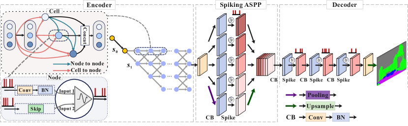
Figure 1: Overall architecture of the spiking encoder-decoder network. The encoder utilizes both cell and layer levels for its search. Each cell comprises multiple nodes (three nodes are depicted here) and connections between nodes form a directed acyclic graph. Each node, a spiking neuron, merges multiple inputs (two inputs are shown). The yellow circles denote the ”stem” layers. The trellis of individual cells (blue circles) delineates the search space of the layer structure. Gray arrows indicate that the resolution of each layer may be doubled, remain unchanged, or halved in comparison to the resolution of the previous layer, with the selection determined by an additional trainable weight. The spiking ASPP layer in the middle extracts multi-scale features from the encoder and feeds them to a decoder, which consists of a series of spiking convolution and batch normalization (BN) layers. Ultimately, an upsampling layer is employed to recover boundary information and generate the predicted semantic segmentation map.

Consistent with standard practices in dense prediction, we utilize an encoder-decoder architecture, as depicted in Figure 1. Effective architectural variation is paramount for dense estimation networks. To this end, we implement a spike-based hierarchical search method [36] to optimize the encoder on both the cell and layer levels. The encoder, which possesses the majority of the network parameters, is optimized due to its crucial role in feature extraction and the subsequent decoding task.

A cell is characterized as a directed acyclic graph comprising multiple nodes, with its structure reiterated across layers. Each cell receives spike input from the preceding two cells. Each node is a spiking neuron that accepts inputs from earlier cells or nodes within the current cell, combines them post candidate operations, and outputs through a spike activation function. The node can be articulated as:

$$y_{j}=f(\sum_{i}o^{(i,j)}(y_{i})),$$ (4)

where $y_{j}$ signifies the spiking output of node $j$, $f$ is a spike activation function, $y_{i}$ represents the output of a prior node or cell, and $o^{(i,j)}$ designates the operation of directed edge $(i\rightarrow j)$. During the search, each operation is depicted by a weighted average of candidate operations:

$$\bar{o}^{(i,j)}(y_{i})=\sum_{o\in O^{(i,j)}}\frac{\mathrm{exp}(\alpha_{o}^{(i,j)})}{\sum_{o\in O^{(i,j)}}\mathrm{exp}(\alpha_{o}^{(i,j)})}o(y_{i}),$$ (5)

where $O^{(i,j)}$ indicates the set of candidate operations on edge $(i\rightarrow j)$ and $\alpha_{o}^{(i,j)}$ is a trainable continuous variable serving as the corresponding weight of operation $o$.

The encoder structure is searched within a pre-defined L-layer trellis. The spatial resolution of a layer can be downsampled or upsampled by a factor of two, or remain unaltered from the previous layer, as determined by a set of weighting factors trained alongside ${\alpha}$. At the conclusion of the search, an optimized architecture is decoded from the trellis. Nearest interpolation is employed for upsampling operations to ensure a binary feature map. Two spiking stem layers [36] are utilized prior to the encoder for initial channel adaptation and feature extraction.

An Atrous Spatial Pyramid Pooling (ASPP) layer [42] with spiking activation is placed at the conclusion of the encoder to extract multi-scale features. The decoder is designed with three consecutive spiking convolution layers and a final upsampling layer, which retrieves boundary information by learning low-level features. To ensure smooth classification boundaries in the final segmentation results, the output from the last upsampling layer is expressed as floating-point values.

We use two spiking stem layers before the encoder for channel adaptation and feature extraction. The first spiking stem layer consists of a 1 $\times$ 1 convolution, and the second incorporates a 3 $\times$ 3 convolution. Both layers follow a batch normalization operation and, ultimately, a spiking activation function. The batch normalization operation can be integrated into convolution during inference [43]. These spiking stem layers accept 5-channel event frames (one SBT stack) as input and output a 96-channel binary feature map. The decoder consists of three consecutive spiking convolution layers and a $1\times 1$ convolution before the final upsampling layer. The comprehensive network structure is outlined in Table I.

TABLE I: Detailed architecture of the searched spiking encoder-decoder network for DDD17. CBS donates module: 2D convolution $\rightarrow$ batch normalization $\rightarrow$ spiking activation. N donates the number of label class.

Module	Layer	Feature map size $c\times h\times w$
Encoder layers	Stem1	$48\times 200\times 346$
	Stem2	$96\times 100\times 173$
	Cell1	$96\times 100\times 173$
	Cell2	$96\times 100\times 173$
	Cell3	$192\times 50\times 87$
	Cell4	$192\times 50\times 87$
	Cell5	$192\times 50\times 87$
	Cell6	$96\times 100\times 173$
Spiking ASPP	CBS1	$256\times 100\times 173$
	CBS2	$256\times 100\times 173$
	CBS3	$256\times 100\times 173$
	CBS4	$256\times 100\times 173$
	Pooling	$96\times 1\times 1$
	CBS5	$256\times 1\times 1$
	CBS6	$256\times 100\times 173$
Decoder Layers	CBS1	$48\times 50\times 87$
	CBS2	$256\times 50\times 87$
	CBS3	$256\times 50\times 87$
	2D Conv	$N\times 50\times 87$
Upsampling	-	$N\times 200\times 346$

III-C Spiking Spatially-Adaptive Modulation

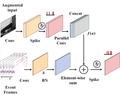
Figure 2: Implementation of Spiking Spatially-Adaptive Modulation (SSAM). The SSAM module employs a dual-path SNN post multiplication-free inference (MFI) to enhance event representation. The augmented input may be original input events, grayscale images, or high-quality RGB images. ‘Conv’ indicates a 2D convolution operation, ‘BN’ signifies batch normalization, ‘Spike’ represents spiking activation, ‘Parallel Conv’ denotes multiple parallel dilated convolutions with differing dilation rates, and ‘Concat’ stands for the concatenation operation. ‘Element-wise sum’ refers to the addition operation performed between feature maps of the upper and lower paths.

Previous research has illustrated that direct application of a convolution and normalization operation stack may result in semantic information being washed out [44]. This issue can be alleviated by enriching the information pathway of the network with lesser normalization [45]. Motivated by this principle, we develop a dual-path SNN with augmented input to amplify event representation. One of the attractive features of SNNs is the multiplication-free inference (MFI), which potentially diminishes computation cost and simplifies hardware design. In alignment with this principle, we devise an MFI-compatible Spiking Spatially-Adaptive Modulation module (SSAM), as illustrated in Figure 2. Let h represent the feature map extracted from input events by convolution, and a denote the augmented input, which could be either original input events or grayscale images. This mechanism is formulated as follows:

$$\hat{h}_{b,c,y,x} =\frac{h_{b,c,y,x}-u_{c}}{\sigma_{c}}+f_{c,y,x}(\textbf{a}),$$ (6)

s $$=S(\hat{\textbf{h}}),$$ (7)

where $b,c,y,x$ symbolize the batch index, channel index, and spatial coordinates respectively; $u_{c}$ and $\sigma_{c}$ represent the mean and standard deviation derived from batch normalization; $f_{c,y,x}(\textbf{a})$ is the learned parameter modulating the event feature through addition at position $(c,y,x)$; $S$ is a spiking activation function; and s is the resultant binary feature map post-modulation. The function generating the modulation parameter is executed with a multi-layer SNN, as demonstrated in Figure 2, where we deploy multi-scale dilated convolution for the parallel convolution and concatenate their feature maps. We also compare different architectural designs in an ablation study. In the experiment, we replace the first stem layer of the encoder with the SSAM. The detailed architecture of the SSAM is provided in the supplementary material.

IV Experiments

We evaluate our methods for event-based semantic segmentation (EbSS) on the benchmark DDD17 dataset [27, 11] and the recently introduced, more expansive DSEC-Semantic dataset [12, 46]. We employ the prevalent loss function and evaluation metrics in semantic segmentation as in [11, 38, 22]. The loss function is defined as the average per-pixel cross-entropy loss:

$$L=-\frac{1}{N}\sum_{i=1}^{N}\sum_{c=1}^{C}y_{i,c}\ln({\hat{y}_{i,c}}),$$ (8)

where $N$ represents the number of labeled pixels, and $C$ is the number of classes. $y{i,c}$ is the ground truth binary value of pixel $i$ belonging to class $c$, and $\hat{y}{i,c}$ is the model predicted probability. We adopt Mean Intersection over Union (MIoU) as the metric for EbSS. Given a predicted image $\hat{y}$ and a ground-truth image $y$, the MIoU is expressed as:

$$\operatorname{MIoU}(y,\hat{y})=\frac{1}{C}\sum_{j=1}^{C}\frac{\sum_{i=1}^{N}\delta\left(y_{i,c},1\right)\delta\left(y_{i,c},\hat{y}_{i,c}\right)}{\sum_{i=1}^{N}\max\left(1,\delta\left(y_{i,c},1\right)+\delta\left(\hat{y}_{i,c},1\right)\right)},$$ (9)

where $\delta$ signifies the Kronecker delta function, and $y_{i}$ specifies the class of pixel $i$.

In the following subsections, we first describe the basic experiment using our encoder-decoder architecture. We then present the ablation study experiments to assess the functionality of the AiLIF neuron and the detailed structure of the SSAM module under various conditions. We also discuss the architecture search and retrain procedures for both the DDD17 and DSEC-Semantic datasets. Furthermore, to highlight the potential advantage of our network in low-power computing, we compare the computational cost of our SNNs with other ANNs. Subsequently, we reveal the results of random seed experiments to ascertain the final architecture. Lastly, we demonstrate how grayscale images provide supplementary information for the semantic segmentation task.

IV-A Experiment on DDD7

[11] introduced the inaugural event-based semantic segmentation dataset based on the DDD17 driving dataset. The dataset includes over 12 hours of DAVIS sensor (346$\times$260 pixel) recordings from both highway and city driving scenarios. The semantic dataset selects six driving sequences from DDD17, chosen based on specific criteria of generated labels such as contrast and exposure. The training set comprises five sequences, while the testing set contains one. The labels cover six classes: flat (road and pavement), background (construction and sky), object, vegetation, human, and vehicle.

IV-A1 Input Representation and Streaming Inference

In real-world scenarios, sensors generate events consecutively over flexible durations. To leverage the potential of SNNs in learningthe temporal correlation of the data, we feed the network with multiple continuous SBT stacks as a stream during training. We correspondingly use successive labels as the target output stream. We set parameters for each stack to $\Delta t=50\mathrm{ms}$, $n=5$, $T=10\mathrm{ms}$, and use four continuous stacks as one input, with the first stack utilized for network warm-up. The corresponding output target is three temporally consecutive labels synchronized with the input. Thus, it effectively outputs one label with one step of simulation. Each input SBT lasts for $50\mathrm{ms}$, and the first column of Figures 4 and 5 displays samples of these, merged in the temporal dimension. During training, the merge window of SBT is $10\mathrm{ms}$ (5 frames as 5 input channels in one stack), thereby retaining sufficient temporal information. Note that this setup naturally allows the SNN to evolve one label in contrast to the multiple time steps required in previous works of SNNs, significantly reducing the training time. For testing inference, we illustrate the real-time applicability of our model by continuously feeding all stacks, which evolve an equal number of steps and output sequential segmentation results.

For the AiLIF neuron, we use $\beta=0.07$ and $\tau_{a}$ with an initial value of 0.3 and limited to [0.2, 0.4] during training. This corresponds to a maximum increase of about 0.1 in the threshold. When using SSAM, we apply the AiLIF neuron to the output spiking layer.

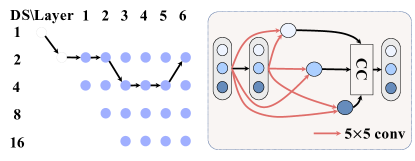
Figure 3: Searched encoder architecture on DDD17. The left figure displays the optimal 6-layer network structure obtained after the search, with the black arrow denoting changes in the network layer resolution. The right figure presents the searched cell structure, where each cell comprises three nodes. The red arrows represent operations between each node and between nodes and cells (5 $\times$ 5 conv), while the black arrows indicate data transfer between cells. DS and CC denote downsample rate and concatenate operation, respectively.

IV-A2 Architecture Search and Retrain

During the encoder search, we randomly partition the training dataset into two sections for bi-level optimization hierarchical search. We incorporate three nodes in a cell with three candidate operations including skip connection, and $3\times 3$ and $5\times 5$ convolution. For the layer search space, we designate the layer number to 6 and adopt a four-level trellis with downsampling rates of 4,2,2,2. We conduct a search over 20 epochs with batch size 2. The first 5 epochs serve to initialize the supernet’s weight, and the subsequent 15 epochs are utilized for bi-level optimization. The search requires about 2 GPU (NVIDIA Tesla V100) days. Figure 3 displays the searched encoder architecture.

During the retraining phase, we randomly initialize the parameters of the searched model and train it for 100 epochs with channel expansion. For the augmented input scenario, we use the same encoder searched on the pure events input. For the SSAM module, we use either the grayscale image or the same event stack with 50 ms in one frame as the augmented input. More details about the architecture and training schedules can be found in the supplementary material.

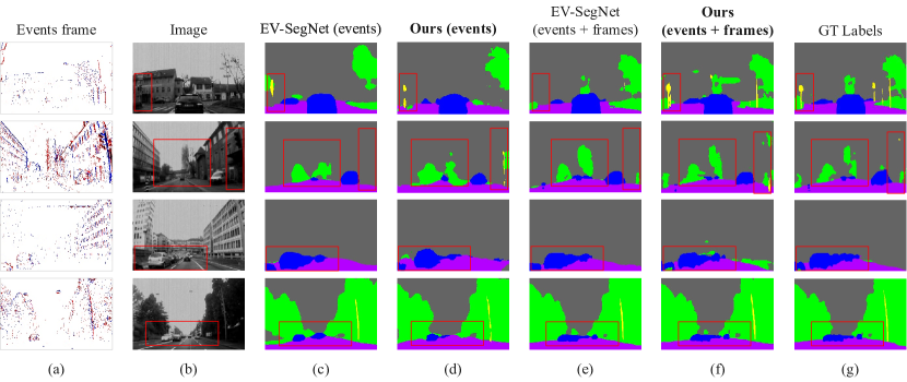
Figure 4: Qualitative comparison on the DDD17 dataset. The red boxes marked in the images indicate where our model’s predictions more closely align with the ground truth labels. Figures in column (a) represent visualizations of event data after applying the SBT method. Diagrams in column (b) display the corresponding grayscale original images. Columns (c) and (d) compare the predictions of EV-SegNet and our model using only event data, respectively. Columns (e) and (f) depict the results of semantic segmentation obtained by utilizing both grayscale images and events. The last column (g) contains the ground truth labels. Images from EV-SegNet are sourced from their paper, while our results are based on the SSAM method.

IV-A3 Results

We compare our methods with state-of-the-art event-based semantic segmentation methods of both ANNs and SNNs, including Spiking-Deeplab/FCN [22], Ev-SegNet [11], ESS [12], and Evdistill [29] as shown in Table II. Among directly training methods, our model with SSAM improves the MIoU by almost 19% with pure events input and 38% with augmented grayscale image over the current record SNN. This is achieved with a smaller network size and only one time-step for convergence.

For combined input, our model also outperforms the current best ANN by 4%, even though the ANN’s network is three times larger than ours. Replacing the first stem layer with SSAM significantly improves network performance for both inputs with grayscale images, underscoring its effectiveness. Although ESS achieves the highest accuracy with pure events input using transfer learning, its performance is suboptimal for combined input. Note that the SSAM module is an effective dual-path SNN compatible with MFI, which also enhances network performance (almost a 2% improvement) even in the absence of grayscale image input. A qualitative comparison between generated semantic segmentation images can be found in Figure 4.

TABLE II: Results on the DDD17 Dataset. E denotes events, F denotes gray-scale image, KD denotes knowledge distillation methods with transfer learning from image datasets.

Method	Type	Input	Time steps	Params (M)	MIoU (%)
Evdistill	ANN	$\text{E}^{\text{KD}}$	-	5.81	58.02
ESS	ANN	$\text{E}^{\text{KD}}$	-	6.69	61.37
Ev-SegNet	ANN	E	-	29.09	54.81
Spiking-DeepLab	SNN	E	20	4.14	33.7
Spiking-FCN	SNN	E	20	13.60	34.2
Ours	SNN	E	1	8.50	51.39
Ours (SSAM)	SNN	E	1	8.6	53.15
ESS	ANN	$\text{E+F}^{\text{KD}}$	-	6.69	60.43
Ev-SegNet	ANN	E+F	-	29.09	68.36
Ours	SNN	E+F	1	8.50	61.84
Ours (SSAM)	SNN	E+F	1	8.62	72.57

IV-B Experiment on DSEC-Semantic

The DSEC-Semantic dataset [12] is derived from the DSEC dataset [46], encompassing recordings from urban and rural environments. It includes 640x440 pixel labels from 11 classes: background, building, fence, person, pole, road, sidewalk, vegetation, car, wall, and traffic sign. The labels from DSEC are of higher quality and greater detail compared to DDD17. We follow the same procedure as [12] for splitting the training and testing sets.

We employ the same network for DSEC-Semantic as we used for DDD17, training it directly on the DSEC-Semantic dataset. In both input configurations, our SNNs outperform the ESS [12] approach, which is augmented with transfer learning. For input that combines events and frames, our network achieves a mean intersection over union (MIoU) of 57.22%, surpassing ESS by 4%. These results attest to the scalability of our architecture for higher-resolution event-based vision tasks. A qualitative comparison of the generated estimations is provided in Figure 5. It can be observed that the SNN, which combines events and frames as input, captures certain details (in the marked area) more accurately than other methods.

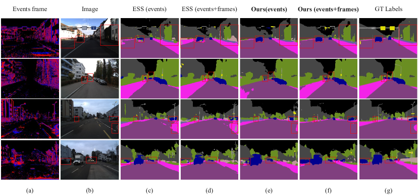
Figure 5: Qualitative comparison on the DSEC-Semantic dataset. Our network, which combines events and frames as input, accurately captures certain details (marked area) better than other methods. The red boxes in the images denote areas where our model’s predictions closely match the ground truth labels. Figures in columns (a) and (b) represent visualizations of event data and RGB images, respectively. Diagrams in columns (c) and (d) depict the results of the ESS method with purely event-based input and combined event and image inputs, respectively. Columns (e) and (f) compare the predictions of our model using solely event data and a combination of RGB images and events (with the SSAM model), respectively. The last column (g) contains the ground truth labels.

TABLE III: Results on the DSEC Dataset. E denotes events, F denotes gray-scale image, KD denotes knowledge distillation methods with transfer learning from image datasets.

Method	Type	Input	Time steps	Params (M)	MIoU (%)
ESS	ANN	$\text{E}^{\text{KD}}$	-	6.69	51.57
Ours (LIF)	SNN	E	1	8.50	52.71
Ours (AiLIF)	SNN	E	1	8.50	53.04
ESS	ANN	$\text{E+F}^{\text{KD}}$	-	6.69	53.27
Ours (SSAM+LIF)	SNN	E+F	1	8.63	57.22
Ours (SSAM+AiLIF)	SNN	E+F	1	8.63	57.77

IV-C Ablation Study

In order to validate the design decisions underlying our architecture and to better understand the individual contributions of various components to the overall performance, we conduct an extensive ablation study. This investigation consists of two parts. In the first part, we examine the influence of the AiLIF neuron, specifically the adaptive threshold, on processing dynamic events. We compare its performance against the standard LIF neuron under a range of base thresholds. In the second part, we focus on the SSAM architecture, probing its utility for event representation in downstream tasks, and evaluating the effect of different configurations of the upper path on network performance. The details of this study are outlined below.

TABLE IV: Results on the DDD17 dataset when applying different neuron models to the first stem layer under different thresholds.

Neuron	Threshold	MIoU %
LIF	0.3, 0.4, 0.5	50.26, 49.65, 49.43
AiLIF	0.3, 0.4, 0.5	49.33, 51.15, 51.39

IV-C1 AiLIF Neuron

To elucidate the efficacy of the adaptive threshold in event processing, we juxtapose AiLIF with standard iterative LIF neurons across a spectrum of base thresholds. This comparison is achieved by incorporating them individually into the primary layer of the network. The outcomes, obtained using the DDD17 dataset, are summarized in Table IV. The AiLIF neuron surpasses the performance of the LIF neuron across all thresholds ranging from 0.3 to 0.5. This underlines the effectiveness of the adaptive threshold in the dynamic processing of events. For a clearer illustration, we depict in Figure 6 a sequence of input event streams by event density, alongside the activation of various neurons. It becomes apparent that the LIF neuron, with a threshold of 0.4 approximately the upper bound of the adaptive threshold of the AiLIF neuron displays the lowest activation. The activation of the AiLIF neuron (base threshold 0.3) typically falls between the two LIF neurons of boundary thresholds. Importantly, its activation even surpasses the LIF neuron with a 0.3 threshold during the initial peak of event density, signifying the complexity of dynamic modulation.

The comparative results between AiLIF and LIF neurons on the DSEC-Semantic dataset are collated in Table III. Relative to the network using only LIF neurons, the network employing AiLIF neurons in the initial ”stem” layer or the final layer of SSAM achieves enhanced accuracy by 0.55% and 1.2% with and without SSAM, respectively.

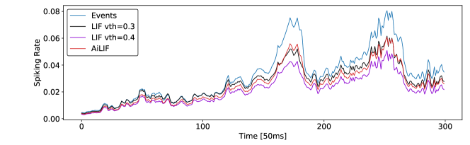
Figure 6: Illustration of event density and activation of AiLIF and LIF neurons in the first stem layer during inference for a short time. The activation of the AiLIF neuron (base threshold 0.3) is generally between the two LIF neurons of boundary thresholds. Note that its activation surpasses the LIF neuron with a 0.3 threshold in the first peak of event density, revealing the intricacy of dynamic modulation.

The study conducted in [21] implemented the ALIF neuron across the entire network, resulting in a suboptimal outcome compared to the use of the LIF neuron. Our experiments replicated this phenomenon, suggesting that excessive flexibility may compromise training precision. Consequently, we restricted the application of AiLIF neurons to the first layer to directly encode events. This significantly improved network performance, showcasing a more efficient utilization of adaptive thresholds for event modulation. As depicted in Figure 7, the self-adaptive threshold of the AiLIF neuron also results in a smoother distribution of spiking rates in the first layer.

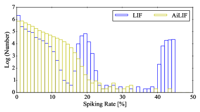
Figure 7: Distribution of spiking rates of LIF neurons (the blue bar) and AiLIF neurons (the yellow bar)in the first stem layer. The horizontal axis represents the spiking rate, while the vertical axis donates the number of neurons in a specific discharge rate range. Moreover, the vertical axis utilizes a logarithmic scale with a base of 10.

IV-C2 SSAM Architecture

The dual-path design of the SSAM module can substitute for the first stem layer of the encoder to enhance event representation for downstream tasks. The module receives 5-channel event frames for the lower path and 1-channel augmented data (gray-scale image or the same event stack with 50 ms in one frame) for the upper path. The module emits a 64-channel binary feature map while retaining the same spatial resolution as the original input. The architecture of the remaining network components remains unchanged from the preceding section. The detailed structure of the SSAM module is presented in Table V.

TABLE V: Detailed operations of SSAM. BN donates batch normalization. The feature maps from the two paths are fused by addition following a spike activation.

Path	Layer Description	Feature map size
Upper	2D conv. $1\times 3\times 3\times 64$ with BN	$64\times 200\times 346$
	Spike activation	$64\times 200\times 346$
	Parallel conv. ($4\times 2D$ conv. $64\times 3\times 3\times$ 16 with dilation {1, 2, 3, 4} and concatenation)	$64\times 200\times 346$
Lower	2D conv. $5\times 1\times 1\times 64$ with BN	$64\times 200\times 346$

In addition, we evaluate network performances with different upper path structures in SSAM under combined input scenarios, including S1: 1 layer of convolution; S2: parallel convolution $\rightarrow$ spiking activation $\rightarrow$ convolution; S3: convolution $\rightarrow$ spiking activation $\rightarrow$ parallel convolution. The various SSAM architectures, encompassing upper path structures S1 and S2, are portrayed in Figure 8a and 8b, respectively.

(a) Upper path structure S1 of SSAM.

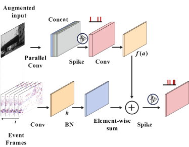
(b) Upper path structure S2 of SSAM.

Figure 8: Illustration of the SSAM upper path structures S1 and S2. The upper path can accommodate various inputs, such as original event data, grayscale images, or high-quality RGB images. Here, ‘Parallel Conv’ refers to several concurrent dilated convolutions with differing dilation rates. ‘Conv’ denotes a 2D convolution operation, ‘BN’ signifies batch normalization, ‘Spike’ indicates spiking activation, ‘Concat’ refers to the concatenation operation, and ‘Element-wise sum’ implies an addition operation conducted between the feature maps of the upper and lower paths. Specifically, structure S1 consists of a single convolution layer, while structure S2 comprises a sequence of parallel convolution, spiking activation, and convolution operations.

The results, compiled in Table VI, indicate that our structure, i.e., S3, outperforms the alternatives. Moreover, the inclusion of a batch normalization layer after the convolution layer in S1 led to a decrease in network performance by 1%. This underscores the soundness of the SSAM’s design principle.

TABLE VI: Results comparison on the DDD17 dataset with different SSAM architectures.

Upper path structure	S1	S2	S3
MIoU %	67.54	68.49	72.57

IV-D Architecture Search and Retrain Details for DDD17 and DSEC-Semantic

For the architecture search on DDD17, we utilize an SGD optimizer with a momentum of 0.9, a learning rate of 0.005, and a weight decay of 0.003 for the training of weight parameters. The parameters ${\alpha}$ and ${\beta}$ are optimized using the Adam optimizer with a learning rate of 0.003 and a weight decay of 0.001. The number of output channels, $N$, in the first stem layer is determined by its correlation with the channel number of the node, $F$, and the number of nodes per layer, $B$, denoted as $N=\frac{F}{2}\times B$. We set $F=8$ to control the model’s capacity during the search. After decoding the optimal architecture, we expand $F$ from $8$ to $32$ in the retraining phase to enhance the network’s representational capability, following [37, 38]. The rest of the network also has its channel numbers quadrupled accordingly. For the retraining of weight parameters, we use the Adam optimizer with an initial learning rate of 0.001, momentum parameters of (0.9, 0.999), and employ a learning rate decay strategy of Poly [47].

The optimized network structure identified on DDD17 is presented in Table I. The first stem layer accepts 5-channel event images with a resolution of 200 $\times$ 346 as input and outputs 48-channel spiking feature maps. We employ cell structure as our basic unit to construct our entire encoder structure. For the remainder of the network, we deploy six cells with different layer resolutions as determined during the search. Subsequently, we use an ASPP layer with five parallel dilated convolutions of varying dilation rates, each followed by batch normalization and a spiking activation operation. Finally, a decoder recovers boundary information, and an upsampling layer generates the predicted semantic segmentation map, completing the segmentation process. In this context, $N$ represents the number of label classes, with $N$ being six on DDD17.

For the DSEC-Semantic dataset, we utilize the same network and training parameters as those employed for DDD17. The detailed network structure for DSEC-Semantic is delineated in Table VII. The first stem layer receives DSEC-Semantic events with a higher resolution of 440 $\times$ 640, followed by the same encoder layers, ASPP layers, and decoder layers as in DDD17. The number of label classes for DSEC-Semantic is 11, and the size of the output feature map generated by the network remains consistent with the input.

TABLE VII: Detailed architecture of the spiking encoder-decoder network for DSEC-Semantic. CBS donates module: 2D convolution $\rightarrow$ batch normalization $\rightarrow$ spiking activation. $N$ donates the number of label class.

Module	Layer	Feature map size $c\times h\times w$
Encoder layers	Stem1	$48\times 440\times 640$
	Stem2	$96\times 220\times 320$
	Cell1	$96\times 220\times 320$
	Cell2	$96\times 220\times 320$
	Cell3	$192\times 110\times 160$
	Cell4	$192\times 110\times 160$
	Cell5	$192\times 110\times 160$
	Cell6	$96\times 220\times 320$
Spiking ASPP	CBS1	$256\times 220\times 320$
	CBS2	$256\times 220\times 320$
	CBS3	$256\times 220\times 320$
	CBS4	$256\times 220\times 320$
	Pooling	$96\times 1\times 1$
	CBS5	$256\times 1\times 1$
	CBS6	$256\times 220\times 320$
Decoder Layers	CBS1	$48\times 110\times 160$
	CBS2	$256\times 110\times 160$
	CBS3	$256\times 110\times 160$
	2D Conv	$N\times 110\times 160$
Upsampling	-	$N\times 440\times 640$

IV-E Sparsity and Computation Cost

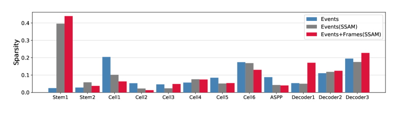
Figure 9: Layer-wise sparsity of SNNs on DDD17. The horizontal axis represents the different layers of the network model, while the vertical axis depicts the spiking sparsity at different layers. ‘Events’ denotes the network without the SSAM block under pure events input. ‘Events (SSAM)’ refers to the network containing SSAM under pure event input, where the enhanced data is also event-based. ‘Events+Frames (SSAM)’ represents a combination of pure events and grayscale image input based on the SSAM network.

TABLE VIII: The operation number and estimated energy cost on DDD17 dataset.SR donates the mean sparsity rate the model.

Method	Input	#Add.	#Mult.	Energy	SR
EV-SegNet (ANN)	E	9322M	9322M	42.88 $\mathrm{mJ}$	-
ESS (ANN)	E	11700M	11700M	53.82 $\mathrm{mJ}$	-
EvDistill (ANN)	E	29730M	29730M	136.76 $\mathrm{mJ}$	-
Ours (LIF)	E	5766M	17M	5.27 $\mathrm{mJ}$	0.077
Ours (AiLIF)	E	5179M	17M	4.74 $\mathrm{mJ}$	0.069
Ours (SSAM+AiLIF)	E	7314M	66M	6.89 $\mathrm{mJ}$	0.092
Ours (SSAM+AiLIF)	E+F	7211M	62M	6.78 $\mathrm{mJ}$	0.091

TABLE IX: The operation number and estimated energy cost on DSEC dataset.

Method	Input	#Add.	#Mult.	Energy	SR
ESS (ANN)	E	46850M	46850M	215.51 $\mathrm{mJ}$	-
Ours	E	32527M	68M	29.59 $\mathrm{mJ}$	0.105
Ours (SSAM)	E+F	27912M	576M	27.77 $\mathrm{mJ}$	0.086

Compared to ANNs, which are based on dense matrix multiplication, SNNs perform event-driven sparse computation, potentially offering advantages in low-power computing. In this section, we compare the computation cost of our SNNs with that of conventional ANNs. As Figure 9 demonstrates, SNNs exhibit sparse activation with varying degrees across layers. The SSAM block significantly enhances event representation by increasing the spiking activation of the first stem layer for both input scenarios. In the decoder, as the activity propagates, layer sparsity decreases, resulting in dense predictions.

As our SNN executes full spike-based computation, its inference involves only addition operations in synapses. Following [18, 16, 22], we compute the number of addition operations of the SNN by $sTA$, where $s$ is the mean sparsity over the entire test set, $T$ is the simulation time step, and $A$ is the addition number in an ANN with an equivalent architecture. For convolution, the addition number $A_{conv}$ can be formulated as

$$A_{conv}=k^{2}\times H_{\text{out }}\times W_{\text{out }}\times C_{\text{in }}\times C_{\text{out }}$$ (10)

where $k$ signifies the kernel size, $H_{out}$ and $W_{out}$ represent the height and width of the output feature map, and $C_{in}$ and $C_{out}$ denote the number of input and output channels.

A minor fraction of multiplication operations is required in the first convolution layer to precisely process input data with floating-point values generated by the SBT method. Notably, all inputs are considered as floating-point numbers when calculating energy consumption, the same approach being used for frame inputs.

The number of multiplication operations is calculated by $T*A$, where $T$ is the simulation time step and $A$ is the multiplication number, which is identical to the addition number for the convolution operation.

The computation costs for both the DDD17 and the DSEC-semantic datasets are outlined in Tables VIII and IX, respectively. Our SNNs register significantly fewer operation numbers than ANNs. Owing to streaming inference, the SNN exploits its temporal dynamics naturally with $T=1$. We estimate the energy consumption following the study of [48] on $45\mathrm{nm}$ CMOS technology used by previous works [18, 16, 22]. The addition operation in the SNN requires $0.9\mathrm{pJ}$, while the multiply-accumulate (MAC) operation in ANNs consumes $4.6\mathrm{pJ}$. Consequently, our SNNs consume $6-28\times$ less energy than ANNs. It is noteworthy that the evaluation of SNNs’ energy efficiency is an active research topic and is heavily dependent on specific hardware. The approach we adopt here facilitates direct comparisons with ANNs. Alternatives, such as SynOps [6], could serve as another viable evaluation method for energy efficiency.

IV-F Random Seed Experiments

In order to determine the final architecture, we replicate the experiment four times with distinct random seeds, selecting the most optimal architecture based on the validation performance achieved by a brief training from scratch. We conduct the search for 20 epochs, with the initial five epochs reserved for weight initialization and the remaining 15 epochs for bi-level optimization. The optimal architecture identified during this iteration is retained in the 1st, 7th, 14th, and 20th epochs. Subsequent to the search, we retrain the model with channel expansion for 50 epochs with a mini-batch size of 2, utilizing the Adam optimizer with an initial learning rate of $0.001$ and momentum $(0.9,0.999)$, along with a learning rate decay strategy of Poly. The search process resulted in an approximate network performance improvement of 19% (from no search to a search lasting 15 epochs). Table X reveals that although the architecture exhibits a degree of sensitivity to initialization, it can be gradually optimized during the search phase. This step-by-step improvement in semantic segmentation can be attributed, to an extent, to the layer-level optimization. A smooth enhancement of the architecture is observed during the search phase.

TABLE X: Search process of the encoder architecture on DDD17. Mean MIoU means the average value of 4 random seeds for the same epoch of 1th, 7th, 14th and 20th , respectively.

Search epochs	1	7	14	20
Mean MIoU %	29.78	29.90	34.96	35.13

IV-G Gray-scale images

Event-based sensors exhibit superior performance in high-speed scenarios and highly dynamic scenes, including under or over-exposure situations, where traditional cameras may fail to provide valid input. On the other hand, the clear images produced by traditional cameras can augment event-based data with finer spatial information. As demonstrated by the IoU in various classes with and without gray-scale images (refer to Table XI), the inclusion of gray-scale images primarily contributes to improving the identification and representation of smaller objects, thereby producing cleaner edge contours. This is particularly noticeable for the classes ‘human’ and ‘vehicle’, which see marked IoU improvements of 35.82% and 28.57% respectively upon the integration of gray-scale images. These enhancements are further supported by the qualitative comparisons illustrated in Figure 3.

TABLE XI: Comparison of IoU for different categories on DDD17 with and without grayscale images, based on the network structure illustrated in Figure 3.

Classes	Flat	Background	Object	Vegetation	Human	Vehicle
IoU(E) %	75.48	88.27	6.41	48.96	22.49	54.38
IoU(E+F) %	90.91	95.01	33.18	75.04	58.31	82.97
Difference	15.42	6.74	26.77	26.08	35.82	28.59

V Conclusions

This study presented a novel architecture for SNNs explicitly developed to handle event-based semantic segmentation tasks. This architecture leverages the unique characteristics of SNNs, which inherently operate through event-driven sparse computation, thereby providing potential for low power applications.

The proposed architecture has been extensively evaluated on two key datasets, DDD17 and DSEC-Semantic. The outcomes of these evaluations consistently highlighted the superior balance achieved between computational expense and task accuracy. In comparison to conventional ANNs, the SNNs exhibited markedly lower operation numbers and considerably reduced energy consumption. These attributes render the proposed SNN architecture highly suitable for resource-constrained and low-power applications. Furthermore, the study also investigated the impact of varying initialization states by conducting experiments with different random seeds. These experiments indicated that the architecture exhibits a steady optimization progression throughout the search phase, leading to an incremental improvement in the performance of semantic segmentation. Additionally, the utility of incorporating grayscale images into the input data was examined. The experimental results suggested a positive impact on the finer details of object representation, particularly with respect to smaller objects, leading to a more accurate depiction of edge contours.

In summary, this research work successfully demonstrates the utility of applying SNNs and DNAS in the sphere of event-based semantic segmentation. It provides strong evidence that these methods can significantly enhance the performance of event-driven vision systems, both in terms of efficiency and effectiveness. While these findings are promising, it is acknowledged that further research is required to realize the full potential of these novel architectures and methodologies in an ever-growing field of study.

References

- [1] T. Serrano-Gotarredona and B. Linares-Barranco, “A 128 128 1.5 contrast sensitivity 0.9 fpn 3 s latency 4 mw asynchronous frame-free dynamic vision sensor using transimpedance preamplifiers,” IEEE Journal of Solid-State Circuits, vol. 48, no. 3, pp. 827–838, 2013.
- [2] C. Brandli, R. Berner, M. Yang, S.-C. Liu, and T. Delbruck, “A 240 180 130 db 3 s latency global shutter spatiotemporal vision sensor,” IEEE Journal of Solid-State Circuits, vol. 49, no. 10, pp. 2333–2341, 2014.
- [3] B. Son, Y. Suh, S. Kim, H. Jung, J.-S. Kim, C. Shin, K. Park, K. Lee, J. Park, J. Woo et al., “4.1 a 640 480 dynamic vision sensor with a 9m pixel and 300meps address-event representation,” in 2017 IEEE International Solid-State Circuits Conference (ISSCC). IEEE, 2017, pp. 66–67.
- [4] K. Roy, A. Jaiswal, and P. Panda, “Towards spike-based machine intelligence with neuromorphic computing,” Nature, vol. 575, no. 7784, pp. 607–617, 2019.
- [5] M. Davies, A. Wild, G. Orchard, Y. Sandamirskaya, G. A. F. Guerra, P. Joshi, P. Plank, and S. R. Risbud, “Advancing neuromorphic computing with loihi: A survey of results and outlook,” Proceedings of the IEEE, vol. 109, no. 5, pp. 911–934, 2021.
- [6] P. A. Merolla, J. V. Arthur, R. Alvarez-Icaza, A. S. Cassidy, J. Sawada, F. Akopyan, B. L. Jackson, N. Imam, C. Guo, Y. Nakamura et al., “A million spiking-neuron integrated circuit with a scalable communication network and interface,” Science, vol. 345, no. 6197, pp. 668–673, 2014.
- [7] S. B. Furber, F. Galluppi, S. Temple, and L. A. Plana, “The spinnaker project,” Proceedings of the IEEE, vol. 102, no. 5, pp. 652–665, 2014.
- [8] A. F. Kungl, S. Schmitt, J. Klähn, P. Müller, A. Baumbach, D. Dold, A. Kugele, E. Müller, C. Koke, M. Kleider et al., “Accelerated physical emulation of bayesian inference in spiking neural networks,” Frontiers in neuroscience, p. 1201, 2019.
- [9] S. H. Ahmed, H. W. Jang, S. N. Uddin, and Y. J. Jung, “Deep event stereo leveraged by event-to-image translation,” in Proceedings of the AAAI Conference on Artificial Intelligence, vol. 35, no. 2, 2021, pp. 882–890.
- [10] K. Zhang, K. Che, J. Zhang, J. Cheng, Z. Zhang, Q. Guo, and L. Leng, “Discrete time convolution for fast event-based stereo,” in Proceedings of the IEEE/CVF Conference on Computer Vision and Pattern Recognition, 2022, pp. 8676–8686.
- [11] I. Alonso and A. C. Murillo, “Ev-segnet: Semantic segmentation for event-based cameras,” in Proceedings of the IEEE/CVF Conference on Computer Vision and Pattern Recognition Workshops, 2019, pp. 0–0.
- [12] Z. Sun, N. Messikommer, D. Gehrig, and D. Scaramuzza, “Ess: Learning event-based semantic segmentation from still images,” in European Conference on Computer Vision. Springer, 2022, pp. 341–357.
- [13] F. Zenke and S. Ganguli, “Superspike: Supervised learning in multilayer spiking neural networks,” Neural computation, vol. 30, no. 6, pp. 1514–1541, 2018.
- [14] Y. Wu, L. Deng, G. Li, J. Zhu, and L. Shi, “Spatio-temporal backpropagation for training high-performance spiking neural networks,” Frontiers in neuroscience, vol. 12, p. 331, 2018.
- [15] E. O. Neftci, H. Mostafa, and F. Zenke, “Surrogate gradient learning in spiking neural networks: Bringing the power of gradient-based optimization to spiking neural networks,” IEEE Signal Processing Magazine, vol. 36, no. 6, pp. 51–63, 2019.
- [16] N. Rathi and K. Roy, “Diet-snn: A low-latency spiking neural network with direct input encoding and leakage and threshold optimization,” IEEE Transactions on Neural Networks and Learning Systems, 2021.
- [17] H. Zheng, Y. Wu, L. Deng, Y. Hu, and G. Li, “Going deeper with directly-trained larger spiking neural networks,” in Proceedings of the AAAI Conference on Artificial Intelligence, vol. 35, no. 12, 2021, pp. 11 062–11 070.
- [18] Y. Li, Y. Guo, S. Zhang, S. Deng, Y. Hai, and S. Gu, “Differentiable spike: Rethinking gradient-descent for training spiking neural networks,” Advances in Neural Information Processing Systems, vol. 34, 2021.
- [19] W. Fang, Z. Yu, Y. Chen, T. Huang, T. Masquelier, and Y. Tian, “Deep residual learning in spiking neural networks,” Advances in Neural Information Processing Systems, vol. 34, 2021.
- [20] S. Deng, Y. Li, S. Zhang, and S. Gu, “Temporal efficient training of spiking neural network via gradient re-weighting,” arXiv preprint arXiv:2202.11946, 2022.
- [21] J. Hagenaars, F. Paredes-Vallés, and G. De Croon, “Self-supervised learning of event-based optical flow with spiking neural networks,” Advances in Neural Information Processing Systems, vol. 34, 2021.
- [22] Y. Kim, J. Chough, and P. Panda, “Beyond classification: Directly training spiking neural networks for semantic segmentation,” arXiv preprint arXiv:2110.07742, 2021.
- [23] L. Zhu, X. Wang, Y. Chang, J. Li, T. Huang, and Y. Tian, “Event-based video reconstruction via potential-assisted spiking neural network,” arXiv preprint arXiv:2201.10943, 2022.
- [24] A. Vaswani, N. Shazeer, N. Parmar, J. Uszkoreit, L. Jones, A. N. Gomez, Ł. Kaiser, and I. Polosukhin, “Attention is all you need,” Advances in neural information processing systems, vol. 30, 2017.
- [25] J. L. Ba, J. R. Kiros, and G. E. Hinton, “Layer normalization,” arXiv preprint arXiv:1607.06450, 2016.
- [26] D. Ulyanov, A. Vedaldi, and V. Lempitsky, “Instance normalization: The missing ingredient for fast stylization,” arXiv preprint arXiv:1607.08022, 2016.
- [27] J. Binas, D. Neil, S.-C. Liu, and T. Delbruck, “Ddd17: End-to-end davis driving dataset,” arXiv preprint arXiv:1711.01458, 2017.
- [28] F. Chollet, “Xception: Deep learning with depthwise separable convolutions,” in Proceedings of the IEEE conference on computer vision and pattern recognition, 2017, pp. 1251–1258.
- [29] L. Wang, Y. Chae, S.-H. Yoon, T.-K. Kim, and K.-J. Yoon, “Evdistill: Asynchronous events to end-task learning via bidirectional reconstruction-guided cross-modal knowledge distillation,” in Proceedings of the IEEE/CVF Conference on Computer Vision and Pattern Recognition, 2021, pp. 608–619.
- [30] L.-C. Chen, G. Papandreou, I. Kokkinos, K. Murphy, and A. L. Yuille, “Deeplab: Semantic image segmentation with deep convolutional nets, atrous convolution, and fully connected crfs,” IEEE transactions on pattern analysis and machine intelligence, vol. 40, no. 4, pp. 834–848, 2017.
- [31] ——, “Semantic image segmentation with deep convolutional nets and fully connected crfs,” arXiv preprint arXiv:1412.7062, 2014.
- [32] J. Long, E. Shelhamer, and T. Darrell, “Fully convolutional networks for semantic segmentation,” in Proceedings of the IEEE conference on computer vision and pattern recognition, 2015, pp. 3431–3440.
- [33] S. B. Shrestha and G. Orchard, “Slayer: Spike layer error reassignment in time,” Advances in neural information processing systems, vol. 31, 2018.
- [34] Y. Wu, L. Deng, G. Li, J. Zhu, Y. Xie, and L. Shi, “Direct training for spiking neural networks: Faster, larger, better,” in Proceedings of the AAAI Conference on Artificial Intelligence, vol. 33, no. 01, 2019, pp. 1311–1318.
- [35] U. Rançon, J. Cuadrado-Anibarro, B. R. Cottereau, and T. Masquelier, “Stereospike: Depth learning with a spiking neural network,” arXiv preprint arXiv:2109.13751, 2021.
- [36] K. Che, L. Leng, K. Zhang, J. Zhang, Q. Meng, J. Cheng, Q. Guo, and J. Liao, “Differentiable hierarchical and surrogate gradient search for spiking neural networks,” in Advances in Neural Information Processing Systems, 2022. [Online]. Available: https://openreview.net/forum?id=Lr2Z85cdvB
- [37] H. Liu, K. Simonyan, and Y. Yang, “DARTS: Differentiable Architecture Search,” arXiv preprint arXiv:1806.09055, 2018.
- [38] C. Liu, L.-C. Chen, F. Schroff, H. Adam, W. Hua, A. L. Yuille, and L. Fei-Fei, “Auto-DeepLab: Hierarchical Neural Architecture Search for Semantic Image Segmentation,” in 2019 IEEE/CVF Conference on Computer Vision and Pattern Recognition (CVPR). IEEE Computer Society, 2019, pp. 82–92.
- [39] G. Bellec, D. Salaj, A. Subramoney, R. Legenstein, and W. Maass, “Long short-term memory and learning-to-learn in networks of spiking neurons,” Advances in neural information processing systems, vol. 31, 2018.
- [40] G. Bellec, F. Scherr, A. Subramoney, E. Hajek, D. Salaj, R. Legenstein, and W. Maass, “A solution to the learning dilemma for recurrent networks of spiking neurons,” Nature communications, vol. 11, no. 1, p. 3625, 2020.
- [41] L. Wang, Y.-S. Ho, K.-J. Yoon et al., “Event-based high dynamic range image and very high frame rate video generation using conditional generative adversarial networks,” in Proceedings of the IEEE/CVF Conference on Computer Vision and Pattern Recognition, 2019, pp. 10 081–10 090.
- [42] L. Chen, G. Papandreou, F. Schroff, and H. Adam, “Rethinking atrous convolution for semantic image segmentation,” CoRR, vol. abs/1706.05587, 2017. [Online]. Available: http://arxiv.org/abs/1706.05587
- [43] S. Ioffe and C. Szegedy, “Batch normalization: Accelerating deep network training by reducing internal covariate shift,” in International Conference on Machine Learning. PMLR, 2015, pp. 448–456.
- [44] T. Park, M.-Y. Liu, T.-C. Wang, and J.-Y. Zhu, “Semantic image synthesis with spatially-adaptive normalization,” in Proceedings of the IEEE/CVF conference on computer vision and pattern recognition, 2019, pp. 2337–2346.
- [45] P. R. G. Cadena, Y. Qian, C. Wang, and M. Yang, “Spade-e2vid: Spatially-adaptive denormalization for event-based video reconstruction,” IEEE Transactions on Image Processing, vol. 30, pp. 2488–2500, 2021.
- [46] M. Gehrig, W. Aarents, D. Gehrig, and D. Scaramuzza, “Dsec: A stereo event camera dataset for driving scenarios,” IEEE Robotics and Automation Letters, vol. 6, no. 3, pp. 4947–4954, 2021.
- [47] W. Liu, A. Rabinovich, and A. C. Berg, “Parsenet: Looking wider to see better,” arXiv preprint arXiv:1506.04579, 2015.
- [48] M. Horowitz, “1.1 computing’s energy problem (and what we can do about it),” in 2014 IEEE International Solid-State Circuits Conference Digest of Technical Papers (ISSCC). IEEE, 2014, pp. 10–14.