All-microwave and low-cost Lamb shift engineering for a fixed frequency multi-level superconducting qubit

Abstract

It is known that the electromagnetic vacuum is responsible for the Lamb shift, which is a crucial phenomenon in quantum electrodynamics (QED). In circuit QED, the readout or bus resonators that are dispersively coupled can result in a significant Lamb shift of the qubit, much larger than that in the original broadband cases. However, previous approaches or proposals for controlling the Lamb shift in circuit QED demand overheads in circuit designs or non-perturbative renormalization of the system’s eigenbases, which can impose formidable limitations. In this work, we propose and demonstrate an efficient and cost-effective method for controlling the Lamb shift of fixed-frequency transmons. We employ the drive-induced longitudinal coupling between the transmon and resonator. By simply using an off-resonant monochromatic driving near the resonator frequency, we can modify the Lamb shift by $32$ to $-30$ MHz without facing the aforementioned challenges. Our work establishes an efficient way of engineering the fundamental effects of the electromagnetic vacuum and provides greater flexibility in non-parametric frequency controls of multilevel systems. In particular, this Lamb shift engineering scheme enables individually control of the frequency of transmons, even without individual drive lines.

Introduction

The rise of modern quantum electrodynamics (QED) was motivated by the need to comprehend the effects of vacuum [1, 2]. One representative phenomenon that accompanied the development of QED is the Lamb shift, which refers to the renormalization of energy levels induced by the electromagnetic fluctuations of the vacuum. Originally, the Lamb shift concerned systems placed in free space. However, the advent of cavity and circuit-QED [3, 4, 5] inspired studies of engineered vacuum. In particular, in circuit-QED, qubits are almost always accompanied by microwave modes in the strong dispersive regime, and Lamb shifts induced by these resonators take significant portions of the bare transition frequency of the qubits [6, 7, 8, 9, 10, 11, 12]. Thus, controlling Lamb shift offers a variety of applications of engineering the transition frequencies of qubits.

In circuit-QED, controlling Lamb shift requires daunting overheads such as flux-tunability [6, 7, 8, 9], voltage biasing [13], or collective states [14]. Lamb shift can also be controlled without the aforementioned costs using external drivings, as proposed in [17, 16, 18]. Unfortunately, one cannot avoid mixing among the eigenstates in this manner. Consequently, the properties of the systems will undergo unwanted renormalization [19].

In this work, we propose and demonstrate an efficient and easy-to-implement approach for Lamb shift control in a typical circuit-QED configuration comprising a transmon [15] dispersively coupled to a single resonator mode. We introduce strong drive fields off-resonant to both the transmon and resonator, inducing drive-induced longitudinal coupling (DLC). This results in state-dependent frequency shifts of the transmon, which exist only when the resonator mode is dispersively coupled and therefore represent the core principle of Lamb shift engineering. We demonstrate the dramatic tuning of the Lamb shift, minimizing undesired renormalization of other properties except the transmon’s frequency. All the experimental results are explained within our theoretical framework.

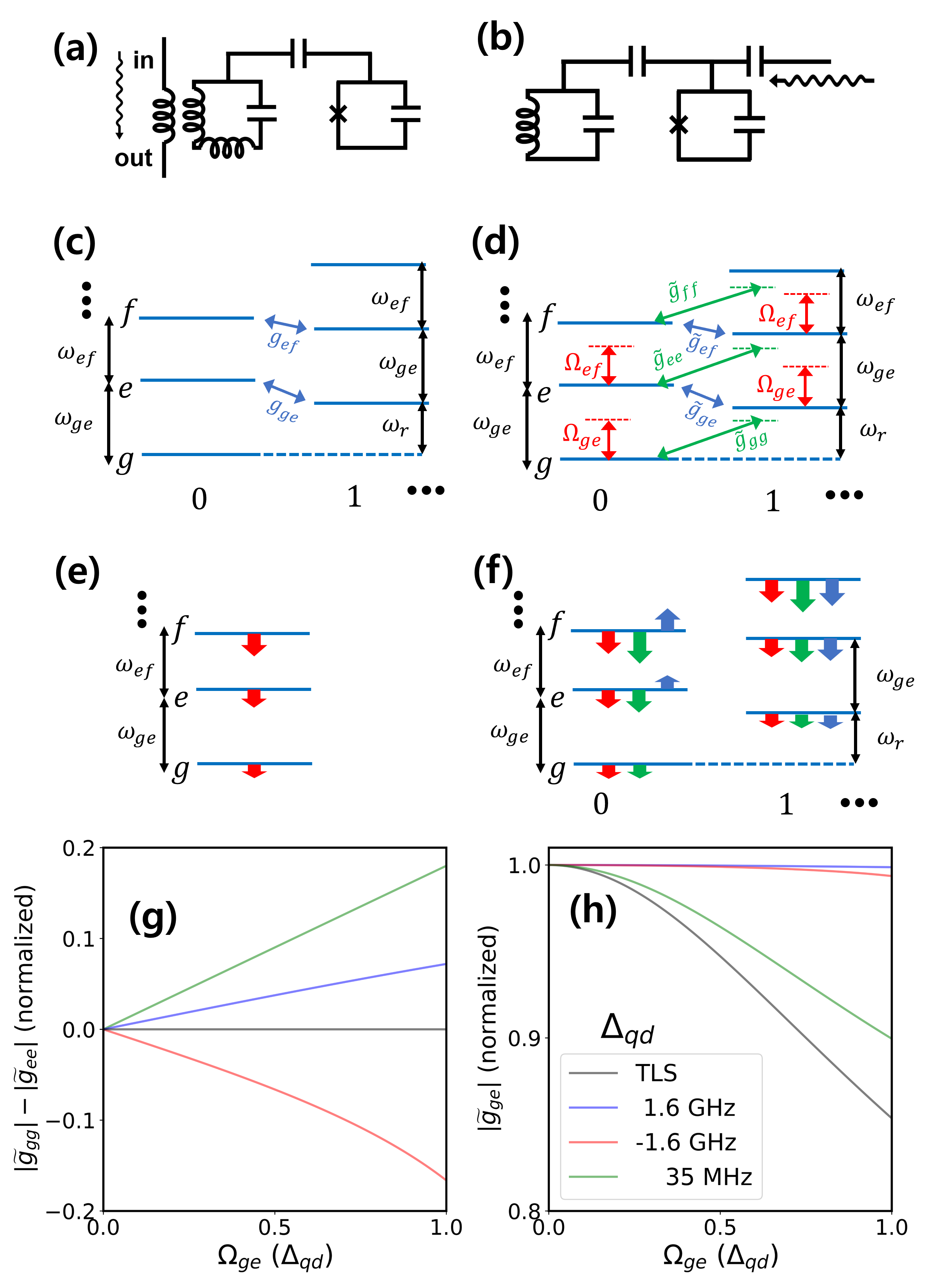
Figure 1: Description of drive-induced Lamb shift engineering. (a) Simplified diagram of circuitry. A transmon is capacitively coupled to a resonator mode. A drive field is inductively applied to the resonator (wavy arrow). (b) Transformed circuitry effectively identical with (a). (c-f) Energy diagram of the system and each horizontal line represent the levels of a bare transmon and resonator. Solid, green, and red arrows denote the effects of static coupling, drive-induced longitudinal coupling (DLC), and AC Stark shift, respectively. (c-d) Major factors accounting for energy level shifts are given by arrows. when a drive field is not present (c) or present (d). (e-f) Graphical description of how each factors shifts energy levels, when the transmon exists alone (e), and coupled with the resonator (f). (g-h) Calculated renormalized coupling matrix elements $\widetilde{g}_{ge},\widetilde{g}_{gg},\widetilde{g}_{ee}$ for several transmon–drive field detunings $\Delta_{qd}$ (red, blue, and green). For a two-state (TS) system (black), $\widetilde{g}_{nm}$ are nearly independent of $\Delta_{qd}$. $\Omega_{ge}$ in x-axis is normalized by $\Delta_{qd}$. The transmon and resonator’s parameters used in the calculation are the same as the experimental values.

Results

Theoretical descriptions

Fig. 1(a) describes an experimental configuration in this work. After applying an appropriate unitary transformation, this configuration becomes equivalent to Fig. 1(b) [19]. The Hamiltonian of the system is then expressed by

$$\begin{split}&\hat{H}=\sum_{n}\omega_{n}\ket{n}_{q}\bra{n}_{q}+i\sum_{n,m}{g}_{nm}\ket{n}_{q}\bra{m}_{q}(\hat{a}-\hat{a}^{\dagger})\\ &+\sum_{n,m}\Omega_{nm}\ket{n}_{q}\bra{m}_{q}\cos(\omega_{d}t)+\omega_{r}\hat{a}^{\dagger}\hat{a}.\end{split}$$ (1)

Here, $\omega_{n}$ and $\ket{n}_{q}$ refer to the energy levels and eigenstates of the transmon. We also express ${\omega}_{n}-{\omega}_{m}={\omega}_{nm}$ for the sake of convenience. We define $\omega_{r}$, $\hat{a}$, and $\ket{n}_{r}$ the resonator frequency, field operator, and eigenstates respectively. We specifically label the zeroth, first, second, and third energy levels of the transmons by $g$, $e$, $f$, and $d$ to distinguish the transmon and resonator modes. The couplings to a resonator and drive field are given by matrices $g_{nm}$ and $\Omega_{nm}$. We consider only the dispersive regime in this work ($|\omega_{nm}-\omega_{r,d}|\gg g_{nm},\Omega_{nm}$). All elements of $g_{nm}$ and $\Omega_{nm}$ are correlated [21]. $g_{ge}$ and $\Omega_{ge}$ are enough to know all the elements.

Each horizontal line in Fig. 1(c-f) represent the levels of the bare transmon and resonator. Fig. 1(c) depicts the $\hat{H}$ when $\Omega_{nm}=0$. Blue arrows indicate the coupling terms that mainly accounts for the energy level shifts. We define ${\omega}_{nm}^{k}$ (${\omega}_{r}^{k}$) the transition frequency of the transmon (resonator) when the resonator (transmon) state is $\ket{k}_{r}$ ($\ket{k}_{q}$). The Lamb shift and resonator frequency pulling can be expressed by $L_{nm}={\omega}_{nm}^{0}-{\omega}_{nm}$ and ${P}={\omega}_{r}^{g}-\omega_{r}$, respectively. For transmons, the same definition is also used in [6, 8, 12]. Interpreting the origin of the Lamb shift in weakly anharmonic systems is of interest in the fundamental perspective [12] but beyond the scope of this work.

We introduce an effective Hamiltonian $\hat{\widetilde{H}}$ [21] equivalent with $\hat{H}$ but presented in a different frame

$$\begin{split}&\hat{\widetilde{H}}\approx\sum_{n}\widetilde{\omega}_{n}\ket{n}_{q}\bra{n}_{q}+\omega_{r}\hat{a}^{\dagger}\hat{a}+\\ &i\sum_{n,m}\widetilde{g}_{nm}(e^{i(n-m+1)\omega_{d}t}-e^{i(n-m-1)\omega_{d}t})\ket{n}_{q}\bra{m}_{q}(\hat{a}-\hat{a}^{\dagger}).\end{split}$$ (2)

$\widetilde{\omega}_{n}$ and $\widetilde{g}_{nm}$ refer to the drive-induced renormalized transmon energy [20] levels and transmon-resonator coupling matrices. We define $\widetilde{\omega}_{nm}^{k}$, which is adiabatically connected to $\omega_{nm}^{k}$ with $\Omega_{nm}\rightarrow 0$. The renormalized Lamb shift and resonator frequency pulling can be expressed by $\widetilde{L}_{nm}=\widetilde{\omega}_{nm}^{0}-\widetilde{\omega}_{nm}$ and $\widetilde{P}=\widetilde{\omega}_{r}^{g}-\omega_{r}$. Let us also express AC Stark shift $\delta\omega_{nm}=\widetilde{\omega}_{nm}-\omega_{nm}$ and $\delta\omega_{nm}^{k}=\widetilde{\omega}_{nm}^{k}-\omega_{nm}^{k}$.

Fig. 1(d) describes the Hamiltonian $\hat{H}$ when $\Omega_{nm}\neq 0$. The arrows indicates major couplings that account for the energy level shifts in our experiment. If $\omega_{d}$ is near $\omega_{r}$ but sufficiently detuned from resonant conditions and any matching frequencies for sideband transitions, only the static coupling (blue) and drive-induced longitudinal coupling (DLC, green) together with the AC Stark shift (red) mainly account for energy level shifts. For transmons, $\widetilde{g}_{nn}\neq\widetilde{g}_{mm}$ when $n\neq m$ in general, and therefore DLC can induce state-dependent shifts of the transmon’s energy levels. The role of DLC is the essence of our Lamb shift engineering scheme. In practical situations, $|\omega_{ge}-\omega_{d}|\gg 1$ is normally satisfied. We then have $\widetilde{g}_{n,n+1}\approx{g}_{n,n+1}$, which means the original coupling between the transmon and resonator is conserved. Furthermore, the energy levels of the transmon are hardly renormalized by DLC, suggesting negligible impact on intrinsic properties of the transmon. This is how the current work is distinguished from our previous work [19], where the significant portions of the Lamb shift renormalization is attributed to the renormalized eigenstates.

Fig. 1(e-f) graphically describe how these factors shift the energy levels. Without the resonator (Fig. 1(e)), only AC stark shift (red) exists. When the resonator mode is coupled to the transmon (Fig. 1(f)), and $\Omega_{nm}=0$, then only the shift by static coupling (blue) exists, and this account for Lamb shift. When $\Omega_{nm}\neq 0$, the shifts by DLC (green) and AC Stark shift appear. AC Stark shift is nearly invariant whether the resonator mode is coupled or not, and consequently contributes negligibly to Lamb shift. On the other hand, the shift by DLC exists only when the resonator mode is coupled to the transmon, acting similarly to additional Lamb shift. Such a role of DLC is beyond the trivial understanding of coupled driven systems, which have not been discussed in the off-resonant drive regime. Our derivation here is given on uncoupled-mode basis, providing more intuitive description for Lamb shift renormalization. We further clarify the non-triviality using normal-mode description in [21].

In Fig.1(g-h), we theoretically calculate some elements of $\widetilde{g}_{nm}$ with respect to $\Delta_{qd}=\omega_{ge}-\omega_{d}$. The device parameters used in the calculation are the same as the experimental values. In Fig.1(g), we observe the discrepancy between $|\widetilde{g}_{gg}|$ and $|\widetilde{g}_{ee}|$ for both far-off-resonant (red and blue) and near-resonant (green) drive fields. For two-state (TS) systems, $|\widetilde{g}_{gg}|=|\widetilde{g}_{ee}|$ always holds, and hence the DLC cannot affect the Lamb shift. Fig.1(h) presents $|\widetilde{g}_{ge}|(=|\widetilde{g}_{eg}|)$, which is proportional to the transition dipole moment between $\ket{g}$ and $\ket{e}$ states and concerns essential properties of the qubit. As we can confirm in Fig.1(h), near-resonant driving significantly renormalizes $\widetilde{g}_{ge}$, whereas far-off-resonant driving hardly affects it. The other components of $\widetilde{g}_{nm}$ not presented in Fig. 1(g-h) give negligible effects when $\omega_{d}$ sufficiently avoids specific conditions for sideband transitions.

Experimental conditions

We obtain the experimental data from two cooldowns. The circuit parameters for each round are distinguished by unbracketed (1st) and bracketed values (2nd). The data in Fig. 2 is obtained 1st round, and Fig. 3 and Fig. 4 is obtained 2nd round. From the pulsed qubit spectroscopy, we obtain $\omega_{ge}^{0}/2\pi\approx 5.901(5.867)$GHz, $\omega_{ef}^{0}/2\pi\approx 5.749(5.715)$GHz, $\omega_{fd}^{0}/2\pi\approx 5.587(5.553)$GHz, and $\omega_{r}^{g}/2\pi\approx 4.290(4.289)$GHz. We also obtain $\omega_{r}/2\pi\approx 4.335(4.335)$GHz by driving the transmon to unconfined states [22]. Based on these, we extract bare qubit parameters and coupling, $\omega_{ge}/2\pi\approx 5.869(5.835)$GHz, $\omega_{ef}/2\pi\approx 5.708(5.676)$GHz, $\omega_{fd}/2\pi\approx 5.539(5.510)$GHz, and $g_{ge}/2\pi\approx 248(245)$MHz. The extracted parameters are consistent with the observed self and cross-nonlinearity, $A=\omega_{ge}^{0}-\omega_{ef}^{0}\approx 2\pi\times 152(150)$MHz and $\chi=\omega_{r}^{g}-\omega_{r}^{e}\approx 2\pi\times 5.8(6.0)$MHz, respectively.

Resolving drive-induced longitudinal coupling

Experimentally verifying the existence of drive-induced longitudinal coupling (DLC) is not trivial. Both DLC and AC Stark shifts yields $\delta\omega_{nm}^{0}\sim O(\Omega_{nm}^{2})$, and thus, one cannot distinguish them just simply measuring the changes in $\omega_{nm}^{0}$ without independent calibration of $\Omega_{nm}$. Instead, we investigate the ratios among $\delta\omega_{nm}^{0}$ to identify the DLC. We introduce the following dimensionless quantities.

$$\begin{split}&\eta_{ef}^{n}=\frac{1}{2}\delta\omega_{gf}^{n}/\delta\omega_{ge}^{n}|_{\Omega_{ge}\rightarrow 0},\\ &\eta_{ed}^{n}=\frac{1}{3}\delta\omega_{gd}^{n}/\delta\omega_{ge}^{n}|_{\Omega_{ge}\rightarrow 0}.\end{split}$$ (3)

We will compare experimentally obtained $\eta$ to the theory with and without considering DLC, and thereby verify the effects of DLC. Note that finding experimental $\eta$ does not demand calibrating $\Omega_{nm}$ since $\eta$’s are independent of $\Omega_{nm}$.

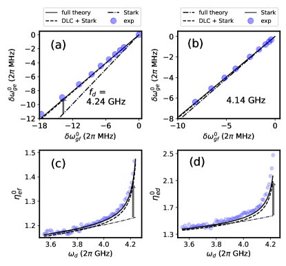
Figure 2: Identifying drive-induced longitudinal coupling (DLC) from multi-level spectroscopy. We investigate $\omega_{d}$ near $\omega_{r}^{g}$, but avoid the resonant condition. Circles and lines denote experimental data and theoretical calculation, respectively. Solid lines are based on Eq. LABEL:eq:dressed_H. In the dot-dashed lines, we exclude the effects of the resonator from Eq. LABEL:eq:dressed_H, which amounts to including only Stark shift in the calculation. Single-dashed lines are based on Eq. LABEL:eq:dressed_H, but we only include the Stark shift and DLC in the calculation. We use Floquet theory for all presented calculations. Gray arrows indicate DLC effects. (a-b) $\delta\omega_{ge}^{0}$ with respect to $\delta\omega_{gf}^{0}$ for $\omega_{d}/2\pi(f_{d})=4.24$ GHz and $\omega_{d}/2\pi(f_{d})=4.14$ GHz, respectively. In (b), although DLC effect exists, we omit a gray arrow just for a visualization problem. (c-d) $\eta_{ef}^{0}$ and $\eta_{ed}^{0}$, while sweeping $\omega_{d}$. See the main text for the definitions and sources of some mismatches between theories and data. Statistical errors in data are negligible, and thus not presented in the plots.

In Fig. 2, we measure both $\eta_{ef}^{0}$ and $\eta_{ed}^{0}$ from multi-level spectroscopy [23]. In Fig. 2(a-b), we present the observed $\delta\omega_{ge}^{0}$ with respect to $\delta\omega_{gf}^{0}$ (circles) for two different drive frequencies near $\omega_{r}^{g}$, 4.24 GHz (a) and 4.14 GHz (b), respectively. We confirm linear correlations among experimentally observed $\delta\omega_{ge,gf,gd}^{0}$ in general with sufficiently small drive powers as seen in Fig. 2(a-b). Lines are linear fits and their slopes are given by $\eta_{ef}^{0}$ (solid and single-dashed) or $\eta_{ef}$ (dot-dashed) based on theories with different Hamiltonian models. In Fig. 2(c-d), we sweep $\omega_{d}$ from 3.55 GHz to 4.25 GHz and present corresponding $\eta_{ef}^{0}$ and $\eta_{ed}^{0}$ from the experiments (circles). The meaning of each lines is the same as in (a-b). For solid lines, we include all component of $g_{nm}$ in Eq. LABEL:eq:dressed_H. For single-dashed lines, we include only the static and DLC terms from the interaction part of the Hamiltonian in Eq. LABEL:eq:dressed_H. In dot-dashed lines, we neglect the renormalization of $g_{nm}$, and therefore these cannot properly capture the changes of Lamb shift. We use Floquet theory [24, 25] for all the theory curves, and the calculation is done by QuTip [26, 27]. See [21] for the detailed numerical method.

In Fig. 2(a-d), we experimentally verify the the effects of DLC shift in $g\rightarrow e,f,d$ transitions. The theory (solid line) based on Eq. LABEL:eq:dressed_H excellently explains the experimental data. The agreements between the solid and single-dashed lines indicate that the DLC mostly accounts for Lamb shift renormalization. Although the discrepancy between data and dot-dashed line seem negligible in Fig. 2(b), they differ by approximately 10%, as shown in Fig. 2(c). More on experimental methods and discussion on small disagreement in between the theory and data is given in [21].

Lamb shift renormalization to the strong drive limit

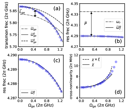
Figure 3: Lamb shift and other renormalized quantities with respect to $\Omega_{ge}$. $\omega_{d}/2\pi=4.2$ GHz for all cases. Circles and lines denote experimental data and theoretical calculation, respectively. All solid lines are based on $\hat{H}$. We use Floquet theory for all presented calculations. (a) An arrow indicates Lamb shift ($\widetilde{L}_{ge}$). The dashed line indicates theoretical calculation based on $\hat{\widetilde{H}}$, but only static couplings are considered ($\overline{\omega}_{ge}^{0}$). (b) An arrow indicates resonator frequency pulling ($\widetilde{P}$). (c) Magnified view of (b). (d) Renormalization of cross-nonlinearity. Dashed line is given by analytical formula with a constant transmon–resonator coupling. See the main text for details and the definition of $\xi$. Statistical errors in data are negligible, and thus not presented in the plots.

In the previous section, we have proven the existence of DLC effects, and thereby learned employing AC Stark shifts alone is an inappropriate approach to calibrate $\Omega_{ge}$. From now on, we use Eq. LABEL:eq:H_s0, including the resonator and interaction terms, to obtain $\Omega_{ge}$ in the experiment. We then quantify the renormalized Lamb shift at large $\Omega_{ge}$ regime in Fig. 3. We cross-check our quantification from the shifts in the resonator frequency and cross-nonlinearity. Note that the AC Stark shift alone cannot explain these shifts simultaneously.

We first obtain the conversion factor $\mu(\omega_{d})$ that satisfies $\mu(\omega_{d})\sqrt{P_{d}}=\Omega_{ge}$, where $P_{d}$ indicates the driving power measured at the signal generator. Fig. 3 present experimentally observed $\widetilde{\omega}_{ge}^{0}$, $\widetilde{\omega}_{r}$, and $\widetilde{\chi}$ (circles) for $\omega_{d}/2\pi=4.2$ GHz. Theoretical expectation (lines) with respect to $\Omega_{ge}$ is also presented. The solid lines refer to the calculated values applying Floquet theory to $\hat{H}$. We set $\mu=138.9$, with which all quantities are simultaneously explained quantitatively.

In Fig. 3(a), an arrow indicates $\widetilde{L}_{ge}$. There is a crossing between the data and dot-dashed line, which means the sign of $\widetilde{L}_{ge}$ is flipped at that drive amplitude. $\widetilde{L}_{ge}$ varies from $32$ to $-30$ MHz in the experiment. whilst $\widetilde{L}_{ge}$ dramatically changes, the change of the resonator frequency pulling $\widetilde{P}$ is relatively less in Fig. 3(b). This result is not surprising since it is already shown in Fig. 1(c) that the DLC cannot directly affect the resonator frequency. Fig. 3(c) is a magnified view of Fig. 3(b).

We present the renormalized cross-nonlinearities ($\widetilde{\chi}$) of the driven transmon–resonator system in Fig. 3(d). The circles and solid-line indicate the experimental and theoretical calculation, respectively. We investigate the origin of $\Omega_{ge}$ dependence of $\widetilde{\chi}$. In perturbation theory, $\widetilde{\chi}$ approximately scales with $\widetilde{g}_{ge}^{2}\widetilde{A}/(\widetilde{\omega}_{ge}-\widetilde{\omega}_{r}-\widetilde{A})$ [15]. For simplicity, we define $\zeta=\widetilde{A}/(\widetilde{\omega}_{ge}-\widetilde{\omega}_{r}-\widetilde{A})$, $\zeta_{0}={A}/({\omega}_{ge}-{\omega}_{r}-{A})$, and $\xi=\zeta/\zeta_{0}$. We observe significant changes of $\widetilde{\chi}$, and this can be approximately quantified by $\chi\xi$ (dashed-line). This manifests the fact that such $\zeta$ rather than $\widetilde{g}_{ge}$ accounts for the changes in $\widetilde{\chi}$, suggesting negligible hybridization among the transmon’s energy levels. We provide a discussion on disagreement among data, solid, and dashed lines at large $\Omega_{ge}$ in [21].

Drive-induced dephasing

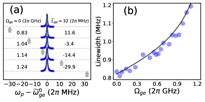
Figure 4: Linewidth broadening by the drive-induced dephasing. $\omega_{d}/2\pi$ is set by 4.2 GHz. (a) The transmon’s two-tone spectroscopy data with respect to various $\Omega_{ge}$. $\omega_{p}$ refers to probe frequency. Corresponding $\widetilde{L}_{ge}$ are also presented. Circles and lines denote data and Lorentzian fits. Gray arrows indicate $\widetilde{\omega}_{ge}$. (b) Extracted linewidths with respect to $\Omega_{ge}$. Line is obtained by theoretical model. The linewidth broadening is originated by the finite lifetime of the resonator and can be suppressed using Purcell filters (see the main text). Statistical errors in (b) are less than the size of symbols, and thus not presented in the plots.

In Fig. 4, we investigate how the transmon’s linewidth varies while engineering $\widetilde{L}_{ge}$ from 32 to $-$30 MHz. Fig. 4(a) shows two-tone spectroscopy of $g\rightarrow e$ transition for various $\Omega_{ge}$. Corresponding $\widetilde{L}_{ge}$ is also presented beside. We obtain $\Gamma_{1}^{q}\approx 1$ MHz and $\Gamma_{\phi}^{q}\approx 2$ MHz from time-domain measurement, where $\Gamma_{1}^{q}$ and $\Gamma_{\phi}^{q}$ are energy relaxation and pure dephasing rates of the transmon. Corresponding linewidth in two-tone spectroscopy is approximately 830 kHz without probe power broadening and measurement-induced dephasing [28, 29]. We also obtain the similar linewidth from two-tone spectroscopy in the experiment, when the calibrated pump strength is approximately 110 kHz, and measurement photon number is far less than unity. There are almost no qualitative changes in the spectrum presented in Fig. 4(a) with increasing $\Omega_{ge}$. However, we notice the linewidth increases by a small amount. Fig. 4(b) shows the extracted linewidth from Lorentzian fitting (circles).

We reveal that the cooperative effects from the driving and finite resonator lifetime can explain the linewidth broadening. We name such effect drive-induced dephasing (DID) in this paper. Such a type of dephasing can be suppressed using resonators with high quality factors or a Purcell filter in the case of resonators with low quality factors. The amount of DID is defined by $\Gamma_{\phi,\textbf{DID}}^{q}$. The same phenomenon is also theoretically predicted in [30], but has been rarely demonstrated experimentally. Based on Eq.33 of [30], we obtain the approximated form of $\Gamma_{\phi,\textbf{DID}}^{q}$

$$\begin{split}\Gamma_{\phi,\textbf{DID}}^{q}\approx\frac{\sqrt{\widetilde{A}\widetilde{\chi}}}{2\widetilde{\Delta}_{rd}}\frac{\Omega_{ge}}{2\widetilde{\Delta}_{qd}}\times\Gamma_{1}^{r}(\omega_{d}).\end{split}$$ (4)

$\widetilde{\Delta}_{qd}$ and $\widetilde{\Delta}_{rd}$ are given by $\widetilde{\omega}_{ge}^{0}-\omega_{d}$ and $\widetilde{\omega}_{r}^{g}-\omega_{d}$, respectively. $\Gamma_{1}^{r}(\omega_{r}^{g})=13.47$ MHz is the resonator decay rate, which is mainly accounted for by the external coupling to the feedline. The theory curve in Fig. 4(b) is based on Eq. 4. $\Gamma_{1}^{r}(\omega_{d})$ is determined by some unknown factors such as the cable resonances of feedlines, and empirically known slowly varying over a few hundreds MHz frequency scale. Thus, we set $\Gamma_{1}^{r}(\omega_{d})$ as a free-fitting parameter and obtain the value of $(0.83\pm 0.05)\times\Gamma_{1}^{r}(\omega_{r}^{g})$ from the least chi-square method. See also extended data in [21].

Discussion

To summarize, we have developed and demonstrated a method for efficient control of the Lamb shift of a fixed-frequency transmon using only a monochromatic microwave drive field. We have verified the renormalization of the Lamb shift through multi-level spectroscopy. By probing the qubit frequencies, cross-nonlinearities, and resonator frequency pullings simultaneously, we have extracted the Lamb shift changes at certain drive amplitudes, which agree excellently with Floquet theory. The Lamb shift varies from $-30$ MHz to $32$ MHz while the interaction strength between the transmon and microwave mode remains nearly constant. Our approach can be implemented to multi-qubit device without any additional complexities. It is applicable beyond the transmon regime as long as we can have significant effects of DLC.

Having controls over the Lamb shift largely concerns in-situ qubit frequency engineering in circuit QED. For fixed frequency qubits, AC Stark shift is the usual approach to tune the frequencies. Drive power and qubit-drive detuning are only the control parameters. Using our scheme adds one more parameter, resonator-drive detuning. This additional degree of freedom is a substantial advantage. Specific application examples are given in [21]. Furthermore, our scheme is cost-efficient, and thus can easily synergize with other applications. In addition, with extended scopes to collective Lamb shift [14] or hybrid systems [31], one can find other applications.

Furthermore, our work will also contribute to precisely sensing the drive amplitudes at device using superconducting qubits. In the relevant previous approaches [23, 32, 33] using superconducting qubits, the operational frequency range are mainly limited to near the resonant frequencies of the qubits. To extend the frequency range to far off-resonant drive regime, taking DLC effects into account is of great importance when the frequencies become closer to the resonators, typically accompany the superconducting qubits.

Author contributions

B.A conceived the study, made the theoretical description, and fabricated the device. B.A also performed the numerical and experimental study. The measurement infrastructure is constructed by G.A.S. B.A. and G.A.S analyzed data. B.A. wrote the manuscript with input from G.A.S.

Data availability

Data supporting the plots within this paper are available through Zenodo at [34]. Further information is available from the corresponding author upon reasonable request.

Supplementary information

S0.1 Theoretical descriptions

S0.1.1 Renormalized interaction – general multi-level systems

The Hamiltonian of a driven general multi-level system is expressed by

$$\begin{split}&\hat{H}_{0}(t)=\sum_{n}\omega_{n}\ket{n}_{q}\bra{n}_{q}+\sum_{n,m}\Omega_{nm}\ket{n}_{q}\bra{m}_{q}\cos(\omega_{d}t).\end{split}$$ (S.1)

Here, $\ket{n}_{q}$ refers to the eigenstates of the undriven multi-level system. The system is $2\pi/\omega_{d}$ periodic in time, and hence we are allow to apply the Floquet theory to calculate the dynamics for arbitrary drive amplitudes $\Omega_{nm}$. In Floquet formalism, quasi-eigenstates and corresponding quasi-eigenenergies for $\hat{H}_{0}(t)$ can be expressed by $\widetilde{\ket{n,\alpha}}_{q}$ = $e^{i\alpha\omega_{d}t}\widetilde{\ket{n,0}}_{q}$ and $\widetilde{\omega}_{n,\alpha}=\widetilde{\omega}_{n,0}+\alpha\omega_{d}$, respectively. Here, $\widetilde{\ket{n,\alpha}}_{q}$ is a Floquet mode with an order of $\alpha$. We also define $\widetilde{\ket{n}}_{q}\in\left\{\widetilde{\ket{n,\alpha}}_{q}\right\}$ and $\widetilde{\omega}_{n}\in\left\{\widetilde{\omega}_{n,\alpha}\right\}$ that is adiabatically connected to $\ket{n}_{q}$ and $\omega_{n}$ with $\Omega_{nm}\rightarrow 0$. The selected Floquet mode $\widetilde{\ket{n}}_{q}$ can be decomposed like

$$\begin{split}\widetilde{\ket{n}}_{q}=\sum_{k}\ket{n}^{(k)}_{q}e^{-ik\omega_{d}t},\end{split}$$ (S.2)

and here $\ket{n}^{(k)}_{q}$ is a Fourier component of $\widetilde{\ket{n}}_{q}$ at frequency $k\omega_{d}$, which also can be decomposed into eigenbases of the undriven transmon $\ket{j}_{q}$ like

$$\begin{split}\ket{n}^{(k)}_{q}=\sum_{j}c_{n,j}^{(k)}\ket{j}_{q}.\end{split}$$ (S.3)

Here, $c_{n,j}^{(k)}$ are time-independent complex numbers. Let us introduce a time-dependent unitary operator $\hat{U}(t)$ satisfying $\widetilde{\ket{n}}_{q}=\hat{U}(t)\ket{n}_{q}$. Under this transformation, $\hat{H}_{0}$ is transformed to

$$\begin{split}&\hat{\widetilde{H}}_{0}=\hat{U}(t)[\hat{H}_{0}-i\partial/\partial{t}]\hat{U}^{\dagger}(t)=\sum_{n}\widetilde{\omega}_{n}\ket{n}_{q}\bra{n}_{q}.\end{split}$$ (S.4)

In addition, the interaction between the general multi-level system and a single mode resonator is given by

$$\begin{split}\hat{{H}}_{I}=i\sum_{n,m}{g}_{nm}\ket{n}_{q}\bra{m}_{q}(\hat{a}-\hat{a}^{\dagger}).\end{split}$$ (S.5)

On the transformed basis, the interaction Hamiltonian $\hat{H}_{I}$ can be given by replacing $\ket{n}_{q}$ with $\widetilde{\ket{n}}_{q}$. Then, we can express the interaction term by

$$\begin{split}&\hat{\widetilde{H}}_{I}=i\sum_{j,j^{\prime}}\sum_{n,m,k,k^{\prime}}g_{nm}c_{m,j^{\prime}}^{(k^{\prime})*}c_{n,j}^{(k)}e^{i(k^{\prime}-k)\omega_{d}t}\ket{j}_{q}\bra{j^{\prime}}_{q}(\hat{a}-\hat{a}^{\dagger}).\end{split}$$ (S.6)

Exchanging $n\rightarrow j$ and $m\rightarrow j^{\prime}$, we can define the time-dependent renormalized interaction matrix $\widetilde{g}_{nm}(t)$ given by

$$\begin{split}&\widetilde{g}_{nm}(t)=\sum_{k,k^{\prime},j,j^{\prime}}g_{jj^{\prime}}c_{j^{\prime},m}^{(k^{\prime})*}c_{j,n}^{(k)}e^{i(k^{\prime}-k)\omega_{d}t}.\end{split}$$ (S.7)

Longitudinal coupling terms appear when $n=m$ is satisfied. Lamb shift control scheme applied to transmons can be also available for the cases where these terms dominate the interaction Hamiltonian. Thus, we do not need to confine ourselves to a transmon case specifically. Generally, $|k^{\prime}-k|$ does not need to be a unity. Specifically for the longitudinal coupling parts ($n=m$) of transmons, however, the terms with $|k^{\prime}-k|=1$ have negligible magnitudes in our parameter regime. Hence we only take $|k^{\prime}-k|=1$ terms into consideration in DLC.

S0.1.2 Renormalized transmon–resonator interaction

A driven transmon is a specific case of Eq. LABEL:eq:H_1-0, where $g_{nm}$ and $\Omega_{nm}$ satisfy the below relation.

$$\begin{split}g_{nn\pm 1}&\approx g_{ge}\sqrt{n+1},\\ g_{nn\pm l}&\approx 0,\\ \Omega_{nn\pm 1}&\approx\Omega_{ge}\sqrt{n\pm 1},\\ \Omega_{nn\pm l}&\approx 0,\end{split}$$ (S.8)

with $l>1$. For transmons under monochromatic transverse drive fields with sufficient detunings and moderate drive amplitudes as in our case, we have

$$\begin{split}c_{n,j}^{(k)}\approx 0\end{split}$$ (S.9)

for $k\pm n\neq j$. Therefore, only the components that meet $k^{\prime}-k=n-m\pm 1$ in Eq. LABEL:eq:H_4 are dominant for transmons, and then the $\widetilde{g}_{nm}(t)$ can be simplified by

$$\begin{split}&\widetilde{g}_{nm}(t)=\sum_{j,j^{\prime}}\sum_{{\begin{subarray}{l}k^{\prime}-k=\\ n-m\pm 1\end{subarray}}}g_{jj^{\prime}}c_{n,j}^{(k^{\prime})*}c_{m,j^{\prime}}^{(k)}e^{i(n-m\pm 1)\omega_{d}t}.\end{split}$$ (S.10)

This simplification can also be justified without using Floquet formalism as presented in our previous works [1]. Dropping oscillating terms, we define the time-independent renormalized interaction matrix $\widetilde{g}_{nm}$

$$\begin{split}&\widetilde{g}_{nm}=\sum_{j,j^{\prime}}\sum_{{\begin{subarray}{l}k^{\prime}-k=\\ n-m\pm 1\end{subarray}}}g_{jj^{\prime}}c_{n,j}^{(k^{\prime})*}c_{m,j^{\prime}}^{(k)}.\end{split}$$ (S.11)

$c_{n,j}^{(k)}$ can be found using Floquet theory in general. However, for weakly anharmonic systems, we can bypass using Floquet theory while not confining ourselves in the conventional approximation regimes. We can calculate $\widetilde{g}_{nm}$ without Floquet theory as presented in our previous work [1]. For the calculation presented in Fig.1 of the main text, therefore, we use the approach in [1], not using Floquet theory to avoid the hardships of finding the proper Floquet mode numbers.

S0.1.3 Normal-mode basis description and non-triviality of DLC-induced Lamb shift engineering.

The transmon’s Hamiltonian can also be expressed using a ladder operator $\hat{b}$, which meets $[\hat{b},\hat{b}^{\dagger}]=1$. Then, $\hat{H}$ defined in the main text can be approximated by

$$\begin{split}\hat{H}\approx~{}\ {\omega}_{q}\hat{b}^{\dagger}\hat{b}+{\omega}_{r}\hat{a}^{\dagger}\hat{a}+g(\hat{a}-\hat{a}^{\dagger})(\hat{b}-\hat{b}^{\dagger})-\frac{E_{c}}{2}(\hat{b}+\hat{b}^{\dagger})^{4}+\frac{\Omega_{ge}}{2}(\hat{b}e^{i\omega_{d}t}+\hat{b}^{\dagger}e^{-i\omega_{d}t}).\end{split}$$ (S.12)

$\omega_{q}$ is the fundamental transition of the transmon in the limit of $E_{c}\rightarrow 0$, where $E_{c}$ is charging energy of the transmon. $g_{ge}$ and $\Omega_{ge}$ refer to the transmon–resonator coupling strength and the drive amplitude on the transmon. Here, the fourth-power term comes from the nonlinearity of the transmon. Higher-order terms are neglected, which is the conventional approximation for transmons. It is often useful to rewrite this Hamiltonian in the normal mode basis. We introduce annihilation operators $\hat{\alpha}$ and $\hat{\beta}$, corresponding to each normal mode. In the dispersive regime, they are given by [6]

$$\begin{split}\hat{a}\simeq&~{}\hat{\alpha}-\frac{g}{\Delta_{qr}}\hat{\beta},\\ \hat{b}\simeq&~{}\frac{g}{\Delta_{qr}}\hat{\alpha}+\hat{\beta}.\end{split}$$ (S.13)

Here, $\Delta_{qr}=\omega_{q}-\omega_{r}$. Then, $\hat{H}$ can be expressed by

$$\begin{split}\hat{H}\approx~{}\,\overline{{\omega}}_{q}\hat{\beta}^{\dagger}\hat{\beta}+\overline{{\omega}}_{r}\hat{\alpha}^{\dagger}\hat{\alpha}-\frac{1}{12}\left[\chi_{r}^{1/4}(\hat{\alpha}+\hat{\alpha}^{\dagger})+\chi_{q}^{1/4}(\hat{\beta}+\hat{\beta}^{\dagger})\right]^{4}+\frac{\Omega_{ge}}{2}(\hat{\beta}e^{i\omega_{d}t}+\hat{\beta}^{\dagger}e^{-i\omega_{d}t}+\frac{g}{\Delta_{qr}}\hat{\alpha}e^{i\omega_{d}t}+\frac{g}{\Delta_{qr}}\hat{\alpha}^{\dagger}e^{-i\omega_{d}t}).\end{split}$$ (S.14)

Here, $\overline{\omega}_{q}$ and $\overline{\omega}_{r}$ are the fundamental transition frequencies of each normal mode in the limit of $E_{c}\rightarrow 0$. The time-dependent terms of Eq. S.14 include driving resonator mode $\hat{\alpha}$. Here, we call this parasitic driving. We apply a unitary transform $\hat{U}=e^{\hat{S}}$ on $\hat{H}$, Here, $\hat{S}(t)=\xi_{q}(t)\hat{\alpha}^{\dagger}-\xi_{q}(t)^{*}\hat{\alpha}+\xi_{r}(t)\hat{\alpha}^{\dagger}-\xi_{r}(t)^{*}\hat{\alpha}$, $\xi_{q}(t)=\frac{\Omega_{ge}}{2(\overline{\omega}_{q}-\omega_{d})}e^{-i\omega_{d}t}$, and $\xi_{r}(t)=\frac{g\Omega_{ge}}{2\Delta_{qr}(\overline{\omega}_{r}-\omega_{d})}e^{-i\omega_{d}t}$. Then, it yields

$$\begin{split}\hat{U}\hat{H}\hat{U}^{\dagger}+i(\partial_{t}\hat{U})\hat{U}^{\dagger}\approx\overline{\omega}_{q}\hat{\beta}^{\dagger}\hat{\beta}+\overline{\omega}_{r}\hat{\alpha}^{\dagger}\hat{\alpha}-\frac{1}{12}\left[\chi_{r}^{1/4}(\hat{\alpha}+\hat{\alpha}^{\dagger}-\xi_{r}(t)-\xi_{r}(t)^{*})+\chi_{q}^{1/4}(\hat{\beta}+\hat{\beta}^{\dagger}-\xi_{q}(t)-\xi_{q}(t)^{*})\right]^{4}.\end{split}$$ (S.15)

Eq. S.15 implies that not only the driving the transmon mode ($\hat{\beta}$), the parasitic driving the resonator mode ($\hat{\alpha}$) can also induce the shift in the transmon frequency. Also, the parasitic driving effect becomes larger as $\omega_{d}$ approaches to $\omega_{r}$. This behavior looks similar with the effect of DLC in uncoupled-mode basis explanation given in the main text. However, we will show that the effect of DLC is irrelavent with the parasitic driving. First, the frequency shift of transmon mode induced by the driving the transmon mode is given by $\delta\omega_{q}=\chi_{q}\frac{\Omega_{ge}^{2}}{(\overline{\omega}_{q}-\omega_{d})^{2}}$. This value approximately corresponds to the red arrow in Fig. 1 of the main text. On the other hand, the shift induced by the parasitic driving is given by $\delta\omega^{\prime}_{q}=2\sqrt{\chi_{q}\chi_{r}}\frac{g^{2}\Omega_{ge}^{2}}{4\Delta_{qr}^{2}(\overline{\omega}_{r}-\omega_{d})^{2}}$. For transmons, $\chi_{q}\approx A$ and $\sqrt{\chi_{q}\chi_{r}}\approx\chi/2$, where $A$ and $\chi$ are defined in the main text. Furthermore, $\chi\approx 2Ag^{2}/\Delta_{qr}^{2}$ is approximately satisfied. The ratio between $\delta\omega^{\prime}_{q}$ and $\delta\omega_{q}$ is then given by

$$\begin{split}\frac{\delta\omega^{\prime}_{q}}{\delta\omega_{q}}=\frac{1}{8}{\left(\frac{\chi}{A}\right)}^{2}{\left(\frac{\overline{\omega}_{q}-\omega_{d}}{\overline{\omega}_{r}-\omega_{d}}\right)}^{2}.\end{split}$$ (S.16)

Plugging the experimental values in Eq. S.16 yields roughly 0.05 when $\omega_{d}/2\pi=4.2GHz$. However, in Fig. 3a in the main text, we already prove the shift induced by DLC is comparable to AC Stark shift. In conventional circuit QED device, $\chi/A\sim 10^{-2}$ and $\overline{\omega}_{q}-\overline{\omega}_{r}\sim 2\pi\times 1$ GHz. This yields $\frac{\delta\omega^{\prime}_{q}}{\delta\omega_{q}}$ less than $10^{-2}$ with $\overline{\omega}_{r}-\omega_{d}=2\pi\times 100$ MHz. Thus, the parastic driving hardly accounts for the total changes of Lamb shift observed in our work.

To summarize, the effects of DLC should not be confused with the trivial parasitic drive effects. In normal-mode description, what approximately correspond to DLC are the terms proportional to $\hat{\alpha}^{(\dagger)}\hat{\beta}^{\dagger}\hat{\beta}$ from Eq. S.15. The effects of these terms have been largely unexplored in the off-resonant drive regime. In the other regime, a few studies have been reported [7, 8], which demonstrate efficient qubit readouts when $\omega_{d}=\widetilde{\omega}_{r}^{g}$. These works have entirely different focus with ours. Normal-mode description is less efficient to intuitively see renormalization of Lamb shift. Thus, we stop our investigation here without further quantitative study on the correspondence between uncoupled-mode and normal-mode descriptions.

S0.2 Numerical and experimental methods

S0.2.1 Eigenenergy calculation

In this work, we utilize QuTiP to apply Floquet theory to the driven Hamiltonian models presented in the main text. Our goal is to find the quasi-eigenenergies of the driven Hamiltonians ($\widetilde{E}_{n,\alpha_{n}}$) that are adiabatically connected to the eigenenergies of the undriven Hamiltonians (${E}_{n}$) when the drive amplitudes are turned off ($\Omega_{ge}\rightarrow 0$). We use the ‘floquet modes’ method of QuTiP, which returns the quasi-eigenenergies in the first Floquet Brillouin zone of the given Hamiltonian, i.e., $\widetilde{E}_{n,0}$ for all $n$. However, these values are not sequentially arranged with respect to $n$, and the sequence even changes as $\Omega_{ge}$ varies. Therefore, we need to take additional steps to find the proper Floquet mode number $\alpha_{n}$ and quasi-eigenenergies. We gradually increase $\Omega_{ge}$ with a sufficiently small step size and, at every step, find the proper $\widetilde{E}_{n,0}$ and corresponding $\alpha_{n}$ such that they are adiabatically connected to the values obtained in the previous step. At the beginning, when $\Omega_{ge}=0$ is satisfied, we can find ${E}_{n}$ using the ‘eigenenergies’ method without Floquet theory, and therefore finding the proper mode numbers is unnecessary. We properly adjust the step size when increasing $\Omega_{ge}$ to balance accuracy and computation time.

S0.2.2 Measurement system

The device and cryogenic setup used in this work are identical to those in our previous work [1]. The device consists of a transmon coupled to two coplanar waveguide resonators, but only one of the resonators is used in this work because the other one is weakly coupled with a cross-nonlinearity of less than 100 kHz, and therefore not effective in the experiments. The transmon and resonators are defined on a 100 nm niobium titanium nitride (NbTiN) film on a 525 $\mu m$ thick silicon substrate [2]. The Al-AlOx-Al Josephson junction of the transmon is fabricated by typical double-angle shadow evaporation. The device is mounted on the mixing chamber plate of a dilution fridge (LD-400) and shielded from radiation and magnetic field using Cooper and Aluminum cans.

Two types of experiments are performed in this work: two-tone spectroscopy using a 4-port vector network analyzer (Keysight N5222A) and pulsed spectroscopy using a Quantum Machines OPX. A signal generator (Keysight N5183B) is used to apply drive fields to the transmon. For pulsed spectroscopy, a 20$\mu s$ transmon excitation pulse is followed by a 2$\mu s$ readout pulse. The transmon excitation pulse is up-converted to RF band using IQ modulation mode of a Rohde-Schwarz SGS100A. The readout pulses are up/down-converted to RF/IF band by IQ mixers. Local oscillator signals of IQ mixers are provided by Rohde-Schwarz SGS100A and Keysight E8257D.

The data in Fig.2, Fig.S1, and Fig.S3 are obtained through pulsed spectroscopy, while the others are acquired through two-tone spectroscopy. Pulsed spectroscopy is preferred for multi-photon transitions as it generally gives signals with better contrasts, but there is a risk of imperfect mixer calibrations. To avoid this, mixer calibration is performed from time to time during the experiments. Two-tone spectroscopy is not efficient for multi-photon transition spectroscopy due to the measurement-induced dephasing, particularly for the $g\rightarrow d$ transition, where it is nearly unavailable. However, two-tone spectroscopy does not require mixer calibration.

S0.2.3 Multi-level transmon spectroscopy

Fig. S1 shows the experimental result of wideband multi-level spectroscopy to find the transmon’s undriven energy levels. We probe the transmon’s second and third excited energy levels by inducing two-photon $g\rightarrow f$ and three-photon $g\rightarrow d$ transitions, respectively.

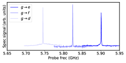
Figure S1: Wideband multi-level spectroscopy of the undriven transmon used in this work.

Once we find the peaks without driving as in Fig. S1, we trace the resonant frequencies as increasing the power of the driving field. In this step, we sweep the probe around expected transition frequencies with much narrower scanning ranges down to a few MHz. The calibrated probe field amplitudes in the frequency $\Omega_{p}$ for $g\rightarrow e$, $g\rightarrow f$, and $g\rightarrow d$ transitions are $2\pi\times 155$ kHz, $2\pi\times 6.92$ MHz, and $2\pi\times 13.86$ MHz, respectively. We determine the proper probe field amplitudes for the multi-photon transitions by compromising the efficiency of the measurement and avoiding undesired sideband transitions between the transmon and resonator. The probe field alone has negligible impacts on the experiment unless the frequency is very close to the matching conditions for the sideband transitions between the resonator and transmon accidentally. In such situations, the probe can induce unexpected frequency shifts of the transmon and resonator. See Fig. S2 for the numerical simulation that supports our statement. We simulate the probe power effect on $g\rightarrow d$ transition spectroscopy without regarding any sideband transition effect between the transmon and resonator.

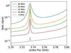
Figure S2: Numerical simulation of probe power effect in $g\rightarrow d$ transition spectroscopy. We sweep the probe amplitude from 5 to 30 MHz in the simulation while sweeping the probe frequency near the $g\rightarrow d$ transition. The locations of the peaks are nearly invariant. The changes in the backgrounds are the effect of $g\rightarrow f$ transition. The effect of undesired sideband transitions between the resonator and transmon is not considered in the simulation.

The frequency of the probe field is close to the resonant frequency $\omega_{q}$ of the transmon, and therefore typically far from the frequency matching conditions for sideband transitions. We should also steer clear of scenarios in which certain combinations of the probe and drive frequencies satisfy undesired frequency matching conditions for sideband transitions. Such situations can cause significant discrepancies between theoretical predictions and experimental results. Fortunately, in this work, our experimental parameters are far removed from such conditions.

S0.2.4 Discussion on theory–experiment mismatches

One can identify irregular fluctuations of the experimental data in Fig. 2(c-d) of the main text. We attribute these to the slow drift of the transmon’s frequencies during the measurement. We cannot use high probe powers for spectroscopy to minimize the undesired couplings induced by probe and drive tones. The poor contrast in the spectrum due to the small probe tone forces us to take averaging for many hours.

Disagreement between solid and dashed lines at large $\Omega_{ge}$ can be attributed to undesired sideband transitions between the transmon and resonator. We strongly suspect three-photon transition $\ket{d}_{q}\ket{0}_{r}$ $\leftrightarrow$ $\ket{g}_{q}\ket{1}_{r}$ since $3\omega_{d}=2\pi\times 12.6$ GHz is very closed to the matching condition of this transition in our case. The solid and dashed lines show better agreements for $\omega_{d}/2\pi=4.0$ and $4.1$ GHz (See extended data in [21]). We can also see disagreement between the experimental data and theories with $\Omega_{ge}/2\pi$ larger than 0.8 GHz. This can be attributed to renormalized couplings among the higher levels of the transmon and resonator, or our model’s missing frequency shifts of higher levels due to the unexpected drive-induced couplings to stray modes. These are, however, the matter outside of computational subspace, $\left\{\ket{g},\ket{e}\right\}$, and therefore should not be taken into account in the calculation.

Possible applications

In addition to the fundamental interests, our findings enable the efficient tuning of both AC Stark and Lamb shifts simultaneously, which is particularly important for non-parametric frequency control of multi-level systems. The ability to control both AC Stark and Lamb shifts offers greater flexibility. In this section, we will introduce specific examples of possible applications.

S0.2.5 Qubit frequency tuning with a global charge line

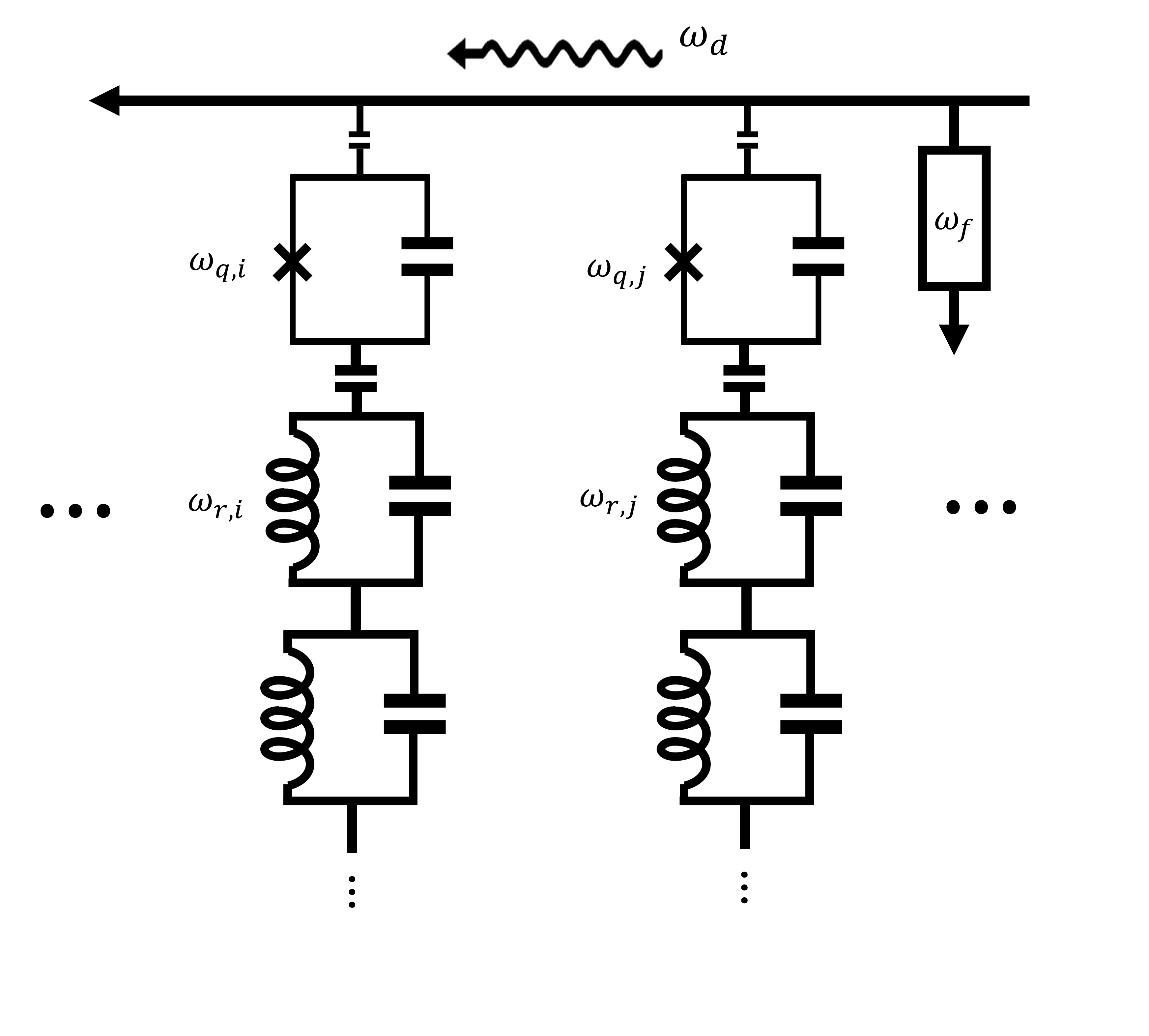
Figure S3: Schematic of qubit frequency tuning with a global charge line . Multiple superconducting qubits ($\omega_{q,n},n=0,1,...$) coupled to a global charge-line (horizontal straight arrow). The qubits are also dispersively coupled to resonator modes (LC circuits), and we use Lamb shift between qubits and resonator modes as additional degree of freedoms for qubit frequency tuning. Only the frequencies of the fundamental mode are presented ($\omega_{r,n},n=0,1,...$). We assume that $\omega_{q,n}$ are confined within a finite frequency band. Individual charge-lines to each qubit, couplers among qubits, readout resonators and readout-lines are not presented for simplicity. A rectangular box represents a filter blocking quantum noise near frequency $\omega_{f}$. We assume $\omega_{f}\approx\omega_{q,n}$.

Standard quantum processors based on fixed-frequency superconducting qubits are accompanied by individually assigned charge-lines to each qubit to implement single qubit gates, and readout resonators coupled to readout lines. The most trivial approach of tuning qubit frequencies is inducing AC Stark shift through each charge-lines. However, the couplings to these charge-lines should be small enough not to induce significant energy loss of the qubits. Furthermore, to avoid undesired renormalization in the strong drive limit, sufficient detunings between the qubits and Stark tones are needed. Introducing additional charge-lines to each qubit with sufficiently large couplings and noise filters around qubit frequencies can be a solution, but this approach requires significant overheads. Applying different AC Stark shifts to each qubit using additional global charge-lines, or readout lines is also not easy since normally the frequencies of qubits and resonators are confined within finite band for hardware efficiency. If some of qubits or readout resonators have similar frequencies, then differently inducing AC Stark shift becomes extremely challenging. The situation becomes more difficult if one wants to have sufficient detunings between the qubits and Stark tones to avoid undesired renormalization.

Our Lamb shift engineering scheme can solve these challenges readily. The proposed circuit design is presented in Fig. S3. An array of qubits is coupled to a global charge-line (horizontal arrow). A filter blocking quantum noise near frequency $\omega_{f}$ is installed. At the same time, qubits are dispersively coupled to the additional resonator modes depicted by LC circuits. We label the frequency of the fundamental modes by $\omega_{r,n}$ ($n=0,1,...$). We also denote the coupling between the qubit and fundamental modes by $g_{qr,n}$ ($n=0,1,...$). Here, readout resonators, readout-lines, couplers among the qubits, and individual charge-lines are omitted in the schematic. Let us assume that $\omega_{q,n}$ ($n=0,1,...$) are similar. By setting $\omega_{f}\approx\omega_{q,n}$, we can protect qubits from the noise channel made by the global charge-line. Thus, we can have sufficient coupling between the qubits and charge-line. There is almost no constrain in choosing $\omega_{r,n}$ and $g_{r,n}$ as long as they are in the dispersive regime. If we set $\omega_{d}$ close to $\omega_{r,i}$, but far-off resonant with $\omega_{r,n},n\neq i$. Then, only qubit $i$ will undergo different frequency shift due to the renormalization of Lamb shift. One can have more options to choose $\omega_{d}$ if using the other higher-order modes (LC circuits without mentioning frequencies beside).

Based on this approach, one can individually regulate the frequencies of multiple qubits using a single drive line, reducing the design complexities of multi-qubit devices and thereby improving the integrity of superconducting qubits. One of the greatest merits of this approach is that all the additional resonators do not need to have couplings to the global charge-line and any of other feedlines. Thus, the global charge-line and additional resonator modes can be easily designed without considering Purcell effect and undesired coupling. This dramatically simplifies the realization of circuits. Furthermore, for ordinary circuit QED systems, implementing more resonators does not make any fabrication overhead.

S0.2.6 Usage with qubit–resonator tunable couplers

Currently, tunable couplers are actively being investigated to enable more efficient on-demand Hamiltonian engineering [5]. The dispersive coupling between qubits and resonators, currently achieved through static capacitance, could potentially be replaced by tunable couplers in the future. This would allow for complete turning off of the coupling when it is not desired, which would be useful in minimizing unwanted cross-talk among qubits and resonators.

However, this plan will encounter challenges due to the back-action on the qubit frequencies that occur when the interaction is turned on. Turning on the coupling not only produces the desired effects but also leads to changes in the qubit frequencies, even when the resonators are empty due to Lamb shift. Avoiding such back-action solely through controlling the AC Stark shift requires updating the microwave tones for the AC Stark shift whenever the coupling is turned on and off. Furthermore, if the back-action shifts the qubit frequency downward, then a compensating Stark tone should be placed in the straddling regime [4], which introduces issues of eigenstate mixing and multi-photon transitions in the strong drive limit.

Obviously, our Lamb shift engineering scheme can overcome all the hurdles mentioned above. If one applies a drive tone with the proper power and frequency, as outlined in our paper, it is possible to keep the qubit frequency unchanged when turning the coupling on and off.

S0.2.7 Efficient engineering transition frequencies of higher energy levels

Due to the weakly anharmonic nature, a transmon’s each transition frequencies undergo simuilar shifts under far-off resonant drive fields. Consequently, the anharmonicities of transmons is relatively more difficult to engineer than fundamental transition frequencies [3]. To overcome this, one should use the drive frequency near resonance of transmons. However in this manner, the drive fields can induce undesired effects such as eigenstate mixing and multi-photon transitions in the strong drive limit.

By utilizing our Lamb shift engineering scheme, it becomes possible to more efficiently tune the higher energy levels of the transmon, even with far-off resonant drive fields. As shown in figure 3d, the anharmonicity of the transmon undergoes a dramatic change, almost doubling in value. This significant tuning of the anharmonicity is primarily caused by the DLC. The underlying principle behind this lies in the fact that the magnitudes of the DLC terms, denoted as $|\tilde{g}_{nn}|$, increase with $n$ for transmons. As a result, each energy level of the transmon experiences a different amount of frequency shift induced by the DLC terms. Therefore, our scheme can also be useful for efficient controls of the higher energy levels of transmons.

Extended data

Extended data sets to reinforce our arguments given in main text are presented in this section.

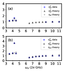
Figure S4: Extended data for figure 2 in the main text. The $g\rightarrow f$ and $g\rightarrow d$ transitions are shown in (a) and (b), respectively. The drive frequency $\omega_{d}/2\pi$ is swept from 3.5 to 11 GHz. We compare the experimental data (circles) with the theoretical calculation (triangles and crosses, respectively). The theory without the vacuum effect (crosses) fails to capture the data around $\omega_{d}\approx\omega_{r}$, clearly indicating the Lamb effect. Please refer to the main text for the definition of $\eta$.

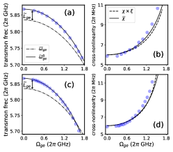
Figure S5: Extended data to figure 3 in main text. We present two cases: $\omega_{d}/2\pi=4.0$ GHz (a,b) and $\omega_{d}/2\pi=4.1$ GHz (c,d). In (a,b) and (c,d), one can clearly identify the changes in the Lamb shift and cross-nonlinearity, respectively. The agreements between the solid and dashed lines in (b) and (d) suggest that the renormalization of the transmon-resonator coupling strength is negligible.

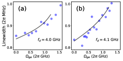
Figure S6: Extended data to figure 4 in main text. We present the cases of $\omega_{d}/2\pi=f_{d}=4.0$ GHz (a) and $\omega_{d}/2\pi=f_{d}=4.1$ GHz (b). The observed linewidth of the transmon is shown with respect to $\Omega_{ge}$ (circles). The theory plots (lines) are based on Eq.3 in the main text, which show good agreement with the experimental data. The proper values of $\Gamma_{1}^{r}(\omega_{d})$ to quantify other data set with $\omega_{d}/2\pi=$ 4.0 and 4.1 GHz seems not dramatically different.

Figure S7: Floquet-based calculation for the case of a transmon coupled with a blue-detuned resonator. In the main text, we only investigated the case of a red-detuned resonator. In this figure, we present numerical studies based on the other configuration. The parameters used for the calculation are identical to the experimental values, except that the resonator frequency is replaced with 7.344 GHz. Depending on the transmon-drive detuning, the Lamb shift varies differently with respect to $\Omega_{ge}$. The drive frequency is 7.5 GHz in (a) and 7.2 GHz in (b).

References

- [1] Byoung-moo Ann, Sercan Deve, Gary A. Steele Resolving Nonperturbative Renormalization of a Microwave-Dressed Weakly Anharmonic Superconducting Qubit Coupled to a Single Quantized Mode, Phys. Rev. Lett. 131, 193605 (2023).
- [2] D. J. Thoen, B. G. C. Bos, E. A. F. Haalebos, T. M. Klapwijk, J. J. A. Baselmans, Akira Endo, Superconducting NbTiN Thin Films with Highly Uniform Properties Over a Ø 100 mm Wafer, IEEE Transactions on Applied Superconductivity, 27, (2017).
- [3] Jayameenakshi Venkatraman, Xu Xiao, Rodrigo G. Cortiñas, Alec Eickbusch, and Michel H. Devoret, Static Effective Hamiltonian of a Rapidly Driven Nonlinear System , Phys. Rev. Lett. 129, 100601 (2022).
- [4] J. Koch et al., Charge-insensitive Qubit Design Derived from the Cooper Pair Box, Phys. Rev. A 76, 042319 (2007).
- [5] D. L. Campbell, A. Kamal, L. Ranzani, M. Senatore, M. LaHaye Modular tunable coupler for superconducting qubits, Phys. Rev. Appl. 19, 064043 (2023)
- [6] Mario F. Gely, Gary A. Steele, Daniel Bothner, The nature of the Lamb shift in weakly-anharmonic atoms: from normal mode splitting to quantum fluctuations, Phys. Rev. A 98, 053808 (2018).
- [7] S. Touzard, A. Kou, N. E. Frattini, V. V. Sivak, S. Puri, A. Grimm, L. Frunzio, S. Shankar, and M.H. Devoret, Gated Conditional Displacement Readout of Superconducting Qubits , Phys. Rev. Lett. 122, 080502 (2019).
- [8] Joni Ikonen et al., Qubit Measurement by Multichannel Driving, Phys. Rev. Lett. 122, 080503 (2019).