The Case for Hierarchical Deep Learning Inference at the Network Edge

Abstract.

Resource-constrained Edge Devices (EDs), e.g., IoT sensors and microcontroller units, are expected to make intelligent decisions using Deep Learning (DL) inference at the edge of the network. Toward this end, there is a significant research effort in developing tinyML models – Deep Learning (DL) models with reduced computation and memory storage requirements – that can be embedded on these devices. However, tinyML models have lower inference accuracy. On a different front, DNN partitioning and inference offloading techniques were studied for distributed DL inference between EDs and Edge Servers (ESs). In this paper, we explore Hierarchical Inference (HI), a novel approach proposed in (Moothedath et al., 2023) for performing distributed DL inference at the edge. Under HI, for each data sample, an ED first uses a local algorithm (e.g., a tinyML model) for inference. Depending on the application, if the inference provided by the local algorithm is incorrect or further assistance is required from large DL models on edge or cloud, only then the ED offloads the data sample. At the outset, HI seems infeasible as the ED, in general, cannot know if the local inference is sufficient or not. Nevertheless, we present the feasibility of implementing HI for machine fault detection and image classification applications. We demonstrate its benefits using quantitative analysis and argue that using HI will result in low latency, bandwidth savings, and energy savings in edge AI systems.

1. Introduction

Deep Learning (DL) models are compute and memory intensive and have been traditionally deployed in the cloud. However, recently, an increasing number of applications in Cyber-Physical Systems (CPS), remote healthcare, smart buildings, intelligent transport, etc. use DL inference at the edge of the network. This initiated a major research thrust in developing small-size ML models (S-ML) – ML models with reduced computation and memory storage requirements – and deploying them on resource-constrained Edge Devices (EDs) such as IoT sensors, wearable devices, mobile phones, drones, and robots. Such deployments are enabled by advancements in hardware and the rapid evolution of model compression techniques (Deng et al., 2020; Sanchez-Iborra and Skarmeta, 2020).

Research works on DL inference at the edge can be broadly classified into 1) tinyML, 2) DNN-partitioning, and 3) inference offloading. TinyML research focuses on enabling extremely resource-limited IoT devices such as micro-controller units (MCUs) to perform on-device DL inference using custom-designed S-ML models. Doing inference at the ED using S-ML saves network bandwidth, improves responsiveness and energy efficiency of the system (Zhang et al., 2017a; Fedorov et al., 2019). Recent advances in tinyML research enable sophisticated applications performing tasks on images and audio that go far beyond the prototypical IoT applications that include monitoring environmental conditions (e.g., temperature, carbon dioxide levels, etc.), machine vibrations for predictive maintenance, or visual tasks such as detecting people or animals (Njor et al., 2022). However, tinyML models have relatively poor inference accuracy due to their small size, which limits their generalization capability and robustness to noise.

The authors in (Kang et al., 2017a) proposed DNN partitioning that divides the inference execution of large-size DNNs between an ED and an Edge Server (ES). However, the benefits of this technique were only realized for computationally powerful EDs (such as smartphones) with mobile GPUs (Dong et al., 2021; Ebrahimi et al., 2022). Finally, works on inference/computation offloading propose load-balancing techniques that divide the inference computational load between the ED and the ES (Wang et al., 2019; Ogden and Guo, 2020; Nikoloska and Zlatanov, 2021; Fresa and Champati, 2022).

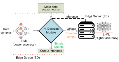
Figure 1. Schematic of HI framework.

a Full Offload

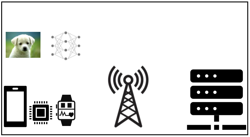
b TinyML

c Inference Offloading

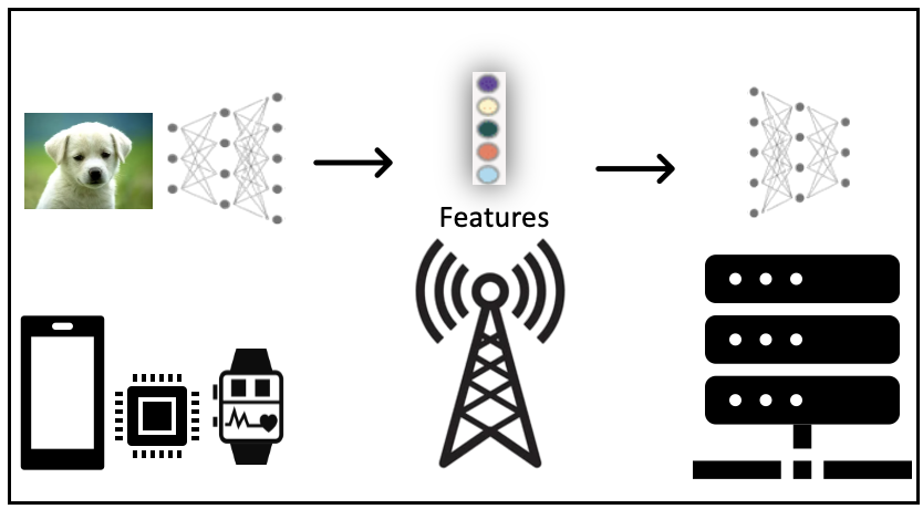
d DNN-partitioning

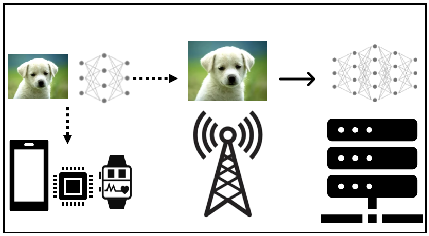
e Hierarchical Inference

Figure 2. Different approaches for DL inference at the Network Edge

In contrast to the above works, we propose Hierarchical Inference, a novel framework for performing distributed DL inference at the edge. Consider the system where the ED is embedded with an S-ML model and enlists the help of ES(s) or cloud on which a stat-of-the-art large-size ML model (L-ML) is available. HI differentiates data samples based on the inference provided by S-ML. A data sample is simple data sample if S-ML inference is sufficient, else it is a complex data sample requiring L-ML inference. The key idea of HI is that only complex data samples should be offloaded to the ES or cloud. Figure 1 shows the HI framework. The HI decision module takes as input the S-ML inference and uses the metadata about S-ML, L-ML, and the application QoS requirements to decide whether a sample is complex or simple and accordingly offload it or not.

Figure 2 illustrate different approaches for DL inference at the edge. In contrast to tinyML research, HI considers inference offloading. Further, HI examines the S-ML inference before making an offloading decision which is in stark contrast to existing inference offloading algorithms. Unlike DNN partitioning, HI is appealing for resource-constrained devices as one may design customized S-ML models for these devices and use off-the-shelf L-ML models on ESs or the cloud.

Advantages of HI

On the one hand, performing inference on EDs saves network bandwidth, improves responsiveness (reduces latency), and increases energy efficiency. On the other hand, doing inference on ESs results in high accuracy inference. HI reaps the benefits of performing inference on EDs without compromising on the accuracy that can be achieved at ESs. To see this, note that HI offloads only complex data samples which need further inference assistance and will (most likely) receive correct inference from L-ML at the ES, while simple data samples which are either redundant or receive correct inference from S-ML are not offloaded, thus saving bandwidth, reducing latency and energy for transmission and computation on L-ML. Although we use the term ‘S-ML’, it need not be an ML algorithm but can be any signal processing or statistical algorithm.

Note that, under HI, performing additional inference locally on all images incurs an extra cost. However, in scenarios where the cost of local computation is lower than that of transmission, this approach would eventually result in significant cost savings, especially since such scenarios are frequent.

Challenges of HI

There are a few challenges to implementing HI.

1. Differentiating simple and complex data samples is the key to HI. However, in general, it is hard to do this differentiation as the ED does not know a priori if the inference output by S-ML is the ground truth or not.

2. There are certain requirements for S-ML in order to enable HI. The S-ML should be small enough in size such that, 1) it should be viable for embedding on ED, 2) the computation energy required for S-ML inference should be less than the transmission energy required for transmitting a data sample, and 3) the S-ML should have reasonable inference accuracy such that for the application of interest the fraction of simple data samples should be higher than that of complex data samples.

Despite the above challenges, in this work, we demonstrate its feasibility by implementing it in three application scenarios: 1) rolling element fault diagnosis, 2) CIFAR-$10$ image classification, and 3) dog breed image classification. The first scenario is a specific example of machine fault detection, where the S-ML is a simple threshold rule on the statistical average of the vibration data. For image classification, we use TFLite and design a customized S-ML for performing inference on images. For each use case, we also provide a quantitative analysis of the benefits of HI. Finally, we also compare the accuracy and delay performance of HI with existing techniques for DL inference: 1) tinyML (no offload), 2) DNN-partitioning, 3) Offloading for Minimizing Delay (OMD), and 4) Offloading for Maximizing Accuracy (OMA).

2. Related Works

Since the advent of AlexNet (Krizhevsky et al., 2012) a decade ago, there has been an explosion in research on bigger DL models with an increasing number of layers and nodes per layer resulting in models with billions of parameters. Examples include the state-of-the-art image classification model BASIC-L (with 2.4 billion parameters) (Chen et al., 2023) and the revolutionary language model chat-GPT (with 175 billion parameters) (Brown et al., 2020). However, large DL models are often over-parameterized and there has been significant research on model compression techniques that reduce the model size by trading accuracy for efficiency, e.g., see (Han et al., 2016; He et al., 2018). Efficient model compression techniques have resulted in mobile-size DL models including SqueezeNets (Iandola et al., 2016), MobileNets (Howard et al., 2017; Sandler et al., 2018), ShuffleNet (Zhang et al., 2017b), and EfficientNet (Tan and Le, 2019). The efforts for designing small-size DL models were further fueled by the need to perform DL inference on edge devices, which span moderately powerful mobile devices to extremely resource-limited MCUs. In the following, we discussed the related work on DL inference at the edge.

TinyML

The tinyML research (Sanchez-Iborra and Skarmeta, 2020) focuses on embedded/on-device ML inference using small-size ML models on extremely resource-constrained EDs such as IoT sensors including micro-controller units (MCUs). The motivation for tinyML stems from the following drawbacks of sending data over a network (Njor et al., 2022): 1) security and privacy of data, 2) unreliable network connection, 3) communication latency, and 4) significant transmission energy consumption. A suite of tinyML models is now available for MCUs enabling a wide variety of complex inference tasks such as image classification, visual wake word, keyword spotting (Banbury et al., 2021), monitoring underwater water environments(Zhao et al., 2022), etc. However, tinyML models have poor inference accuracy (relative to large-size DL models) due to their small size, which limits their generalization capability and robustness to noise. Further, once a tinyML model is trained (on an edge server/cloud) and deployed on an IoT sensor or an MCU, improving its accuracy using active learning on each data sample may not be possible due to the resource constraints of the device. Therefore, to improve inference accuracy the EDs need to offload the data samples by enlisting the help of an Edge Server (ES) or a cloud, where L-ML models are deployed.

DNN Partitioning

For the scenarios where the ED is a powerful mobile device, such as a smartphone, the authors in (Kang et al., 2017a) proposed DNN partitioning, where the front layers of the DNN are deployed on mobile devices while the deep layers are deployed on Edge Servers (ESs) to optimize the communication time or the energy consumption of the mobile device. The premise of this technique is that the data that needs to be transmitted between some intermediate layers of a DNN is much smaller than the initial layers. Following this idea, significant research work has been done that includes DNN partitioning for more general DNN structures under different network settings (Hu et al., 2019; Li et al., 2020) and using heterogeneous EDs (Hu and Li, 2022), among others. However, as we will show later, for DNN partitioning to be beneficial, the processing times of the DNN layers on the mobile device should be small relative to the communication time of the data generated between layers. Thus, works on DNN partitioning (e.g., see (Dong et al., 2021; Ebrahimi et al., 2022)) require mobile GPUs making this technique infeasible for extremely resource-constrained IoT sensors and MCUs.

Inference Offloading

Inference offloading or computation offloading is a load-balancing technique for partitioning the set of data samples between the ED and the ES for computing the inference. It is worth noting that computation offloading between EDs and ESs was extensively studied in the literature, e.g., see (Mach and Becvar, 2017; Feng et al., 2022). However, the majority of the works studied offloading generic computation jobs, and the aspect of accuracy, which is relevant to offloading data samples, has only been studied recently (Wang et al., 2019; Ogden and Guo, 2020; Nikoloska and Zlatanov, 2021; Fresa and Champati, 2022). These works compute offloading decisions using one or more of the following quantities: job execution times, communication times, energy consumption, and average test accuracy of the ML models. Note, however, that the average test accuracy may not be the right indicator for the correct or incorrect inferences provided by an S-ML across different data samples and thus it may result in adversarial cases where most of the data samples that are scheduled on S-ML may receive incorrect inference. In contrast to inference offloading HI first examines the S-ML output to determine if the data sample is simple or complex and only offloads if it is a complex data sample. We note that early exiting within the layers of DNNs, proposed in (Teerapittayanon et al., 2016), received considerable attention recently. This technique could be used in conjunction with the above DL inference approaches, including HI, to further reduce the latency in reference.

In our previous work (Moothedath et al., 2023), we proposed the idea of HI and focused on a specific technique for realizing it for an image classification application by using an existing S-ML model. In contrast, in this paper, we provide a general definition of HI, consider multiple use cases (machine fault detection and dog breed image classification), design S-ML algorithms, and provide a quantitative comparison with existing DL inference at the edge.

3. HI for Rolling Element Fault Diagnosis

In order to demonstrate how HI can be used in machine fault detection we turn to the motor bearing dataset, provided by the Case Western Reserve University (CWRU) bearing data centre, a standard vibration-based dataset used in Rolling Element Bearings (REBs) fault diagnosis (Case Western Reserve University Bearing Dataset, [n.d.]; Smith and Randall, 2015). The failure of REBs is one of the most frequent reasons for the breakdown of rotating machines. In Figure 3, we show an REB that is located at the driver end of the rotating machine. At the other end of it lies the fan end REB. A faulty REB may have a fault on the inner lace or outer lace or in the rolling element.

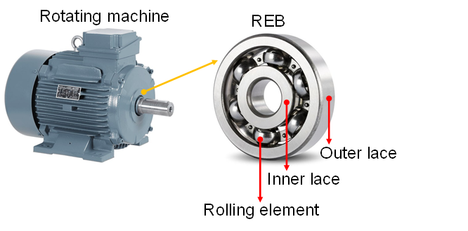
Figure 3. An REB at the driver end of a rotating machine.

The CWRU dataset consists of $161$ datasets, each collected for driver-end REB and fan-end REB under different settings, which includes samples collected at $12$ kHz and $48$ kHz frequencies under varying motor loads ($0-3$ hp), varying shaft speeds ($1730-1797$ rpm), and for three fault widths $0.18$, $0.36$, and $0.54$ mm. For a given motor load and shaft speed, the task is to identify $10$ states of the rotating machine, which include a normal functioning state and nine fault states resulting from three fault widths seeded on each inner lace, outer lace, and ball bearing.

A state-of-the-art CNN proposed in (Wen et al., 2018) identifies each of these states with $99.6$% accuracy. The CNN is trained on $64\times 64$ grey images created from batches of $4096$ consecutive samples. The CNN consists of $8$ layers and it cannot be deployed on resource-constrained sensors to do local inference. Instead, it needs to be deployed on an ES or in the cloud and transmit all the data from the sensors. Consider as an example that a factory floor consists of $100$ rotating machines. Since each rotating machine contains more than two REBs, the bandwidth required to transmit all the data to an ES or cloud (on which the CNN is deployed) in order to monitor the state of all REB is at least $76.8$ Mbps, assuming that the sampling frequency is $48$ kHz and each sample value is stored in a $2$ byte register. The question we ask is: can we achieve $99.6$% accuracy in classifying the states of the REBs without needing to use such high bandwidth?

Figure 4. Time series vibration data averaged over every $4096$ samples for aprox. 120,000 samples collected at $18$ mm fault width.

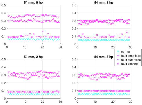
Figure 5. Time series vibration data averaged over every $4096$ samples for aprox. 120,000 samples collected at $54$ mm fault width.

In order to answer the above question, we make a simple observation that the REBs (or in general machines) work in a normal state for hundreds (or thousands) of hours. If we can differentiate normal state from not normal state (any of the faulty states) on the sensor, then we save almost the entire bandwidth by only offloading the samples to CNN when not in the normal state. To this end, we analyzed the CWRU dataset and computed the average for batches of $4096$ consecutive vibration samples with series lengths of approximately $120,000$ from different datasets. Note that to compute the average values a sensor doesn’t need to store all the $4096$ samples. Instead, it can use a simple moving average. In Figures 4 and 5, we plot the average values under normal state (in cyan) and under faulty states (in magenta) for different motor loads at $18$ mm and $54$ mm fault widths, respectively. For the dataset in Figure 4, it is easy to verify that by setting a threshold $0.07$ below which the REB is in normal state and not in normal state, otherwise, provides $100$% accuracy for normal vs not normal classification. Note that this simple threshold rule is the S-ML in our definition of HI. Further, for this scenario, all the states can be classified with $100$% accuracy as the data points are separable via thresholds.

In Figure 5, however, all the states are not separable. In particular, the inner lace and outer lace faults cannot be differentiated using thresholds. Nevertheless, normal and not normal states can still be differentiated using a threshold of $0.07$. Thus, the sensor only transmits data samples that correspond to one of the fault states, which of course can then be classified by the CNN at ES or cloud. Thus, from the above data analysis, we conclude that a sensor can make a local decision about normal state or not normal state of the REB using a basic computation of averages. Since an REB is in normal state for longer periods, significant bandwidth savings can be obtained using HI. It is worth noting that, here the samples collected in the normal state are indeed simple data samples and the samples collected in a faulty state are complex data samples. Furthermore, since computing a moving average is not compute-intensive, the sensor will save all the transmission energy that would have been spent in transmitting the simple data samples. Thus, using HI results in potential energy savings for IoT devices that in turn improves their battery lifetimes.

4. HI for CIFAR-10 Image Classification

We choose Image classification as our second use case as it is a fundamental task inherent to a variety of applications including object detection, image analysis, video analytics, and remote sensing. Significant efforts have been devoted to developing advanced classification approaches and techniques aiming to improve classification accuracy (e.g., see (Gong and Howarth, 1992), (FOODY, 1996), (Gallego, 2004)). We choose CIFAR-$10$ image dataset consisting of $50,000$ training samples, $10,000$ test samples and $10$ classes. We design and train an S-ML that can be embedded on a resource-constrained ED such as MCU with eflash memory size of order $1$ MB and SRAM of order few hundred KB. The details of the ML models are given below.

• S-ML: We build a convolutional neural network (CNN) with five layers: a convolutional layer, a max-pooling layer, a flatten layer, and two fully-connected dense layers. We use tensorFlow’s Keras API to train it on the CIFAR-$10$ dataset. Our final quantized TFLite mode has an inference accuracy of $62.58\%$ and is $0.45$ MB, a size suitable for deploying on MCUs.

• L-ML: Many existing state-of-the-art DNN models have already demonstrated top-1 accuracy on the CIFAR-$10$ dataset, in particular, with some models achieving up to $99.5\%$ (Dosovitskiy et al., 2020). For this work, we choose EfficeintNet (Ruseckas, nd), which achieves an accuracy of $95\%$.

Exploring the idea of HI, simple data samples in this context would be the images that the S-ML embedded on the IoT device is able to classify correctly, otherwise they are considered as complex data samples. The data sample will initially undergo inference by the S-ML. The ED will decide to either accept the inference or consider it incorrect and offload the data sample to the L-ML deployed on the ES.
For the ED to make this decision, we use two key ideas proposed in (Moothedath et al., 2023). The first idea is with regard to how to quantify the confidence of the S-ML’s inference. For image classification, a DNN outputs a probability mass function (pmf) over the classes. Note that one can obtain such pmf for other ML classification algorithms (such as linear classifier) by normalizing the output with the sum of the values output for each class. We use the maximum probability value, denoted by $p$, from the pmf as the confidence of S-ML. This is justified because it is a standard approach to declare the class corresponding to the maximum probability $p$ as the true class. The ED will utilize the same metric to examine or track the validity of the S-ML inference and decide whether to accept the inference or delegate it to the L-ML that resides on the ES. This means that the local inference of data sample $i$ will be accepted or rejected based on its associated $p_{i}$. The ED’s decision rule for data sample $i$, denoted by $\delta(i)$, will be based on comparing $p_{i}$ with a threshold $\theta\in[0,1)$:

$$\delta(i)=\left\{\begin{array}[]{lr}\text{Offload}&\text{if }p_{i}<\theta\\ \text{Do not offload}&\text{if }p_{i}\geq\theta\end{array}\right.$$

The second idea adopted from (Moothedath et al., 2023) is the cost model. If the S-ML’s inference is rejected and the data sample $i$ is offloaded to the ES, a fixed cost $0\leq\beta<1$ will be received for offloading. This offloading cost, $\beta$, can be adjusted to consider different factors that may be specific to the context of the task and the user, rather than being limited to a fixed cost tied to a specific metric. In practice, it may correspond to transmission energy consumption or data transfer cost or remote inference delay. We choose to introduce HI using an abstract cost for offloading to enhance flexibility in the decision-making process and make it adaptable to diverse scenarios and requirements. This abstract cost may differ across various setups, allowing our decision algorithm to make more informed decisions that balance various costs and benefits, such as network conditions, resource availability, battery life, and user’s personal preferences. Furthermore, denote by $\eta_{i}$ the additional cost obtained from the ES inference of the data sample $i$. It is equal to $1$ if the L-ML’s inference is incorrect and is equal to $0$, otherwise. Alternatively, if data sample $i$’s accepted local inference is correct, then the incurred cost, denoted by $\gamma_{i}$, is $0$; otherwise, it is $1$. Thus, the cost for data sample $i$ using HI is given by:

$$\mathcal{C}_{i}=\left\{\begin{array}[]{lr}\beta+\eta_{i}&\text{if }p_{i}<\theta\\ \gamma_{i}&\text{if }p_{i}\geq\theta\end{array}\right.$$

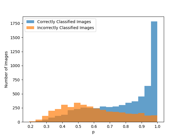
Figure 6. Classification of CIFAR-10 by the S-ML model.

Figure 6 shows the number of correctly and incorrectly classified images of the CIFAR-$10$ dataset using our S-ML model as a function of $p$. The figure clearly illustrates that for $p$ greater than $0.6$, the number of correctly classified images becomes higher than the incorrectly classified ones. Thus, it serves as an appropriate threshold candidate to decide whether to accept the local inference or not. In fact, brute-force search shows that the optimal probability threshold $\theta^{*}$ that yields the minimum cost for CIFAR-10 dataset is $0.607$.

HI Approach: The data samples will be subjected to inference using the S-ML embedded on the ED. The ED will decide to offload only the data whose inference’s associated $p$ is less that the optimal threshold $\theta^{*}=0.607$.

Results and Discussion

Implementing the complete offload approach, which involves running a state-of-the-art DNN on the Edge Server and offloading the whole data $(10000$ images$)$, the ES achieves an accuracy of $95\%$. Only $500$ out of $10000$ images were falsely classified, which is considered a top-tier accuracy. However, it comes at a cost of $10000\,\beta+500$, meaning that this approach is expensive. Conversely, the complete local approach, which involves accepting all of the local inferences produced by the S-ML embedded in the ED, can reduce the cost to $3742$, which is a significant reduction particularly when $\beta$ is large and close to one. However, it entails a significant trade-off in terms of inference accuracy $62.58\%$, which is insufficient to ensure reliability in the majority of use cases.

Following the HI approach with $\theta^{*}=0.607$, only $35.5\%$ of the data is offloaded $(3550$ images$)$ of which $71$ images of them were misclassified by the ES. This yields a cost of $(3550\beta+71)$. Moreover, out of the $6450$ accepted local inferences, $1577$ were misclassified (which contribute an extra $1577$ to the cost). This means that the total cost of HI is $3550\beta+1648$. Since $1648$ images are misclassified under HI, it has $83.52\%$ accuracy. HI can result in a cost reduction of $\big{(}\frac{6450\,\beta-1148}{10000\,\beta+500}\times 100\big{)}\%$ compared to offloading all of the images. Thus, HI can provide the best of both worlds, namely significant cost reduction while still achieving a dependable level of accuracy based on the cost $\beta$. The relative cost reduction for different values of $\beta$, is in the range $14-49\%$.

Approach	No Offload	Full Offload	Hierarchical Inference
Offloaded Images $(\%)$	$0(0\%)$	$10000(100\%)$	$3550(35.5\%)$
Misclassified Images $(\%)$	$3,742(37.42\%)$	$500(5\%)$	$1,577\,\textbf{ON ED}+71\,\textbf{ON ES}\;(16.48\%)$
Accuracy $(\%)$	$62.58\%$	$95\%$	$83.52\%$
Cost $(\beta)$	$3742$	$10000\,\beta+500$	$3550\,\beta+1648$

Table 1. Image classification performance comparison for CIFAR-10 dataset: number of offloaded images, misclassified ones and the total cost.

5. HI for Dog Breed Image Classification

In this section, we introduce another use case that comes in alignment with the concept of hierarchical inference naturally. Suppose that we have the same set-up (ED connected to an ES) and that we are only interested in classifying the dog breeds of the dogs present in CIFAR-$10$. On one hand, achieving high accuracy for this complicated task using tinyML models is still challenging due to the complex nature of dog breed classification and the limited resources of tinyML devices. On the other hand, fully offloading all of the images can result in high accuracy but is, however, very costly. Under HI, we propose to use an S-ML to classify dog images and non-dog images and only offload the dog images to ES for an L-ML to classify the dog breed. Note that, in this use case the dog images are complex as they require further assistance for classification at the ES. All non-dog images are simple.

The approach used in this use case generalizes to contexts where the data samples of interest would be sufficiently complex that almost none of them could be accurately inferred on the edge device. Then, the S-ML will not do any final inference for the data of interest. Instead, its job would be just to eliminate a large part of the irrelevant data and only delegate the data samples of interest. Table 2 summarizes the performance measures and the current use case details vs the previous ones.

Use Case		Rolling Element Fault Diagnosis	CIFAR-10 Image Classification	Dog Breed Classification
Data Description	Simple Data Sample	REB that are in normal state (normal functioning)	Images that would be correctly classified by SML	Images that are irrelevant, do not feature a dog
	Complex Data Sample	REB that are in any faulty state	Images that would be incorrectly classified by SML	Images that are of interest, feature a dog
Cost	Transmission Cost	-	$\beta$ per offloaded image	$\beta$ per offloaded image
	Inference Cost	-	1 per incorrect inference	1 per offloaded irrelevant image
Accuracy		Number of detected REB in faulty state / Total number of REB in faulty state	Number of correct inferences / Total number of images	Number of correctly classified dogs / total number of dogs

Table 2. Data description, cost and accuracy for the presented use cases.

• S-ML: The ED will embed a small binary ML model, where it must be able to recognize whether the image features a dog (and thus of our interest) or not. For the S-ML we train a small-size CNN for binary classification, i.e., dog or not dog. The model consists of five layers: $2D$ convolutional layer, MaxPooling2D layer, flatten layer, and two dense layers. The initial dense layer consists of $32$ neurons, utilizing the ReLU activation function. The final layer is a single neuron using the sigmoid activation function. The S-ML produces $p$, a probability score between $0$ and $1$, indicating the probability of the input image being classified as a positive class, which in this scenario is dogs. To make it adequate for resource-constrained devices, the model is afterwards converted to a quantized TFLite model. The resultant model’s size is $0.23$ MB and has $63.86\%$ accuracy.
  

• L-ML: For this use case, we assume that the L-ML has $100$ % accuracy, and therefore any image that is offloaded will be accurately classified. Once the S-ML classifies the image as a dog image, the ED will offload it to the ES and the correct dog breed will be determined. This assumption is made since the true labels of the dog breeds are not available for CIFAR-$10$ and thus it is necessary to enable us to make a comparison with respect to the ideal accuracy (ES). In fact, it is not an unrealistic assumption to consider a perfect L-ML, as there are multiple models that have already demonstrated exceptional state-of-the-art accuracy in dog breed classification for various datasets (Cui et al., 2023).

For data sample $i$, the S-ML outputs $p_{i}$, the probability that it features a dog. The ED will utilize this probability to decide whether to offload the sample or consider it irrelevant and disregard it. The ED’s objective is to offload only the dog images, and since the SML is a binary classification model, $p=0.5$ serves as a threshold for dog classification and thus the decision rule for data sample $i$, denoted by $\delta(i)$, will be the following:

$$\delta(i)=\left\{\begin{array}[]{lr}\text{Offload}&\text{if }p_{i}\geq 0.5\\ \text{Do not offload}&\text{if }p_{i}<0.5\end{array}\right.$$

If the data sample $i$ has to be offloaded to the ES, the cost received will depend on its L-ML’s inference. A fixed cost $0\leq\beta<1$ will be received for offloading a sample from the dataset of interest (if it was true dog image). Alternatively, if the data sample offloaded was irrelevant (does not feature a dog), a cost of 1 will be incurred.

Figure 7a represents the actual non-dog (simple data samples) and dog images (complex data samples) in our dataset distributed as a function of $p$. The images having $p\geq 0.5$ will be classified as dog images (complex) by the S-ML. The figure clearly shows that most of the dog images were correctly identified by the S-ML, i.e., the precision of the trained S-ML is high. Specifically, only $88$ dog images out of $1000$ dogs are misclassified and are not offloaded. These are the false negatives. This means that for the task of classifying the dog breeds of CIFAR-$10$, $912$ out of $1000$ dogs will be identified by the S-ML and delegated to the L-ML to determine their correct breed. This yields a $91.2\%$ accuracy. Moreover, the figure illustrates that the S-ML will incorrectly classify a substantial number of non-dog images, $3521$ to be precise, as dog images, leading to their unnecessary offloading to the L-ML. These misclassifications are false positives. An important note here is that these false positives will only affect the total cost incurred but not the accuracy of HI. Figure 7b presents the instances of false positives and false negatives as a function of $p$.

Using the full offload approach for such a scenario can yield maximal accuracy, but it comes with a significant cost of $9000\beta$ for offloading irrelevant images. On the other hand, implementing HI can tremendously reduce the accrued cost while maintaining a reliable level of accuracy. Table 3 compares HI with the full-offload approach. Using HI leads to an offload reduction by $55.67\%$ which reduces the cost by $(\frac{88\beta+5479}{10000\beta+9000}\crossproduct 100)\%$ while maintaining an accuracy of $91.2\%$. The relative cost reduction for different values of $\beta$, is in the range $50-60\%$.

From the above use case analysis, we conclude that HI offers a balanced solution that strikes a middle ground between the two extremes of no offload and full offload. On one end, fully offloading the samples can yield maximum accuracy but comes with high costs. On the other end, performing all inferences locally can reduce costs but requires significant compromises in accuracy. HI approach has the potential to offer the best of both worlds, allowing for a significant reduction in costs while still maintaining a reliable level of accuracy.

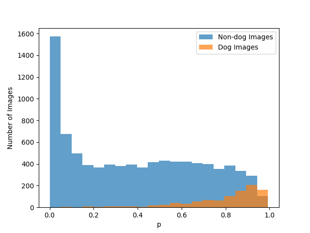
a Non-dog images (simple data samples) and Dog images (complex data samples) of CIFAR-10 dataset as a function of S-ML’s output $p$.

b False Negatives (miss-identified dogs) and False Positives (incorrectly classified as dogs) of CIFAR-$10$ by the S-ML.

Figure 7. Analysis of our S-ML output for dog breed classification.

Approach	Full offload	HI
Number of Offloaded Images	$10,000$	$4,433$
Accuracy $(\%)$	$100\%$	$91.2\%$
Cost	$1000\,\beta+9000$	$912\,\beta+3521$
Cost Reduction $(\%)$	$0\%$	$(\frac{88\beta+5479}{1000\beta+9000}\crossproduct 100)\%$

Table 3. HI binary classification for CIFAR-10 dataset performance comparison with Full offload.

6. Comparison with Existing Approaches

a Throughput of CIFAR-$10$ Image Classification
of different approaches vs $\beta$.

b Accuracy of CIFAR-$10$ Image Classification
of different approaches vs $\beta$.

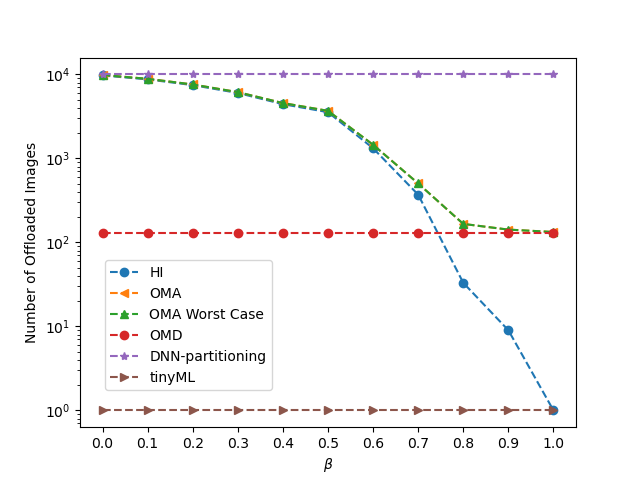
c Number of offloaded Jobs to ES of CIFAR-$10$ Image Classification of different approaches vs $\beta$.

Figure 8. Different approaches comparison for varying $\beta$.

This section presents a comparison of HI with tinyML, two algorithms related to inference offloading, and DNN partitioning. We choose the task of CIFAR-$10$ dataset image classification and throughput, accuracy and number of offloaded images as metrics for our comparison. We begin by introducing these algorithms and describing the experimental setup, followed by a discussion of the results.

1. TinyML: Embedded ML approach where all the inferences of the S-ML are accepted (no offload).

2. Offloading for maximizing accuracy (OMA): computation offloading approach that partitions inference jobs between the ED and the ES for maximizing accuracy given a time constraint. The time constraint we subject is equal to makespan of the HI approach. Two cases are investigated: 1) Partitioning the images between ED and ES randomly, and 2) OMA Worst Case scenario, where the algorithm accepts the local inference for complex samples and offloads the simple ones.

3. Offloading for Minimizing Delay (OMD): computation offloading approach that partitions the set of images such that S-ML and L-ML will have the same makespan resulting in the minimizing the total makespan for processing all images.

4. DNN-partitioning (Kang et al., 2017b): Since the CIFAR-$10$ dataset has $32\times 32$ images, the DNN-partitioning approach results in full offload. Further explanation and measurements of why this approach in our context is equivalent to full offload are provided in the Appendix.

We use the S-ML and L-ML described in Section 4 for all the above approaches. Our S-ML can fit on any IoT device but for the current work, we deploy it on a Raspberry Pi $4B$, which features a single CPU with $4$ cores, a frequency of $1.5\,GHz$, and $5\,GB$ of RAM. As for the L-ML, it is hosted on an ES featuring $2$ CPUs with $16$ cores each, a frequency of $2.4\,GHz$, an NVIDIA Tesla T4 GPU and $256\,GB$ of RAM. Both devices are connected to the same WLAN and are linked via $802.11$ operating on a $5\,GHz$ channel approved by ETSI for Multi-access Edge Computing (MEC) communication. The transmission of images from ED to ES is accomplished through TCP sockets. In order to estimate the communication time, we utilize iPerf to determine the communication bandwidth. We conduct a total of $30$ experiments, each lasting $60$ seconds, to derive our estimates. The average communication bandwidth between Raspberry Pi and ES recorded was $10.45\,MB/s$ (SD = 0.6 $MB/s$). The average inference time per one sample by the S-ML on the Raspberry Pi is $0.99\;msec$, which is significantly lower than the $74.34\;msec$ required to offload the image from the ED to the ES, and to execute the inference on the L-ML on ES with GPU processing.

We compare HI with the various approaches in terms of throughput (relating to the makespan and thus delay), accuracy and the number of offloaded images (which relates to the approach’s cost). Figure 8a (8b) shows the throughput (accuracy) of the four approaches vs HI for different values of $\beta$. Note that $\beta$ has an effect only on the results of HI, but since the chosen time constraint of OMA (and OMA worst case) is equal to the makespan of HI, we see that OMA (and thus OMA worst case) is also sensitive to the choice of $\beta$. Figure 8a shows that tinyML has maximum throughput and OMD has throughput close to tinyML throughput. In addition, tinyML scores the lowest number of offloaded images (lowest cost) but Figure 8b clearly states that their accuracy score is the lowest and not reliable for most of the DL inference tasks. On the other hand, DNN-partitioning has the top accuracy score but it is the worst in terms of throughput and the number of offloaded images. HI and OMA (OMA worst case) have, by design, similar throughput but HI provides significant gains in terms of accuracy and lower number of offloaded images (thus cost) compared to OMA.

Compared to other approaches, HI offers a significant reduction in latency and cost while maintaining high accuracy. In fact, HI approach was found for example to reduce latency and the number of offload images by approximately $63.15\%$ and $64.45\%$ respectively compared to the full offload approach, while still maintaining $83.52\%$ accuracy for $\beta=0.5$. In summary, HI has demonstrated its ability to provide the best of all worlds, including accuracy, delay, and cost. As a result, it represents a promising solution for real-time applications on resource-constrained devices.

7. Conclusion

In conclusion, this paper explored a novel approach, Hierarchical Inference (HI), for performing distributed DL inference between edge devices and edge servers. HI addresses the challenges of resource-constrained EDs in making intelligent decisions using DL inference. Through application use cases and quantitative analysis, we demonstrated the feasibility and benefits of HI. We presented three different use cases for HI: machine fault detection, CIFAR-$10$ dataset image classification and dog breeds classification. We provide a quantitative comparison between HI and existing techniques for DL inference at the edge which include, tinyML, inference offloading and DNN partitioning. Our results demonstrate that HI achieves significant cost savings while maintaining reliable accuracy. For instance, following HI’s approach for CIFAR-$10$ image classification reduces latency and the number of offloaded images compared to the full-offload approach, on average for values of $\beta$ ranging from $0$ to $1$, by $60.84\%$ and $62.179\%$ while maintaining an accuracy greater than $80\%$. With minimal compromise on accuracy, HI achieves low latency, bandwidth savings, and energy savings, making it a promising solution for edge AI systems.

8. APPENDIX

Device	Processing Unit	L1	L2	L3	L4	L5	L6	L7
Raspberry Pi	CPU	328.9	1640.7	1131.7	970	1561	1981	539.8
ES	GPU	1.01	2.51	1.50	2.16	2.31	2.89	0.91

Table 4. Time to process each layer of Efficentnet in milliseconds.

Input	Size (MB)	Time (msec)
Image	$0.003$	[$0.28$,$0.30$]
Output L1	$3.06$	[$276.92$, $310.65$]
Output L2	$1.64$	[$148.41$, $166.49$]
Output L3	$1.13$	[$102.26$, $114.72$]
Output L4	$0.97$	[$87.78$, $98.47$]
Output L5	$1.56$	[$141.17$, $158.37$]
Output L6	$1.98$	[$179.18$, $201.0$]
Output L7	$0.53$	[$47.96$, $53.80$]

Table 5. Communication time between Raspberry Pi and ES measured in milliseconds.

Approach		Time (msec)
No Offload		0.99
Full Offload		74.34
DNN-partitioning	Layer 1	[618.1 , 651.83]
	Layer 2	[2127.78 , 2145.86]
	Layer 3	[3211.83 , 3223.57]
	Layer 4	[4165.19 , 4175.88]
	Layer 5	[5787.27 , 5804.47]
	Layer 6	[7803.39 , 7825.21]
	Layer 7	[8211.06 , 8216.9]

Table 6. Time (in milliseconds) for one inference following different approaches: No Offload, Full Offload and DNN-partitioning at different layers

This section provides an explanation of why DNN-partitioning is considered equivalent to full offload approach in our context. We started by attempting to compare the performance of DNN partitioning when EfficientNet is divided between an Edge Device and an Edge Server. However, after measuring the processing time (as reported in Table 4) and the communication time for offloading the features (as reported in Table 5), we found that it is not feasible to partition the DNN model. Additionally, a single inference on the Edge Device for L-ML takes approximately 8 seconds to execute on the Raspberry Pi, based on the measurements in Table 4. The inference time required for different approaches, i.e., no offloading, full offloading, and DNN-partitioning at each layers, is presented in Table 6. The results indicate that even partitioning at a single layer and deploying a fraction of L-ML at the ED can result in a substantial delay compared to offloading the complete image. For instance, partitioning at a single layer increases the inference time from $74.34$ msec to $[618.1,651.83]$ msec. This proves that DNN-partitioning is not valid in our case and would lead to a full offload approach. It’s worth noting that the output size of each layer in MB is larger than the size of a CIFAR-10 $32\times 32$ image. This is because EfficientNet requires a $224\times 224\times 3$ input, so we up-scaled the CIFAR-10 images using padding. This padding doesn’t affect the semantic content of the image, but it does allow them to be scheduled on EfficientNet. Recall that we chose to use EfficientNet because it’s the state-of-the-art model for the classification problem with the CIFAR-10 dataset.

References

- (1)
- Banbury et al. (2021) Colby Banbury, Vijay Janapa Reddi, Peter Torelli, Nat Jeffries, Csaba Kiraly, Jeremy Holleman, Pietro Montino, David Kanter, Pete Warden, Danilo Pau, Urmish Thakker, antonio torrini, jay cordaro, Giuseppe Di Guglielmo, Javier Duarte, Honson Tran, Nhan Tran, niu wenxu, and xu xuesong. 2021. MLPerf Tiny Benchmark. In Thirty-fifth Conference on Neural Information Processing Systems Datasets and Benchmarks Track (Round 1).
- Brown et al. (2020) Tom B. Brown, Benjamin Mann, Nick Ryder, Melanie Subbiah, Jared Kaplan, Prafulla Dhariwal, Arvind Neelakantan, Pranav Shyam, Girish Sastry, Amanda Askell, Sandhini Agarwal, Ariel Herbert-Voss, Gretchen Krueger, Tom Henighan, Rewon Child, Aditya Ramesh, Daniel M. Ziegler, Jeffrey Wu, Clemens Winter, Christopher Hesse, Mark Chen, Eric Sigler, Mateusz Litwin, Scott Gray, Benjamin Chess, Jack Clark, Christopher Berner, Sam McCandlish, Alec Radford, Ilya Sutskever, and Dario Amodei. 2020. Language Models are Few-Shot Learners. CoRR abs/2005.14165 (2020). arXiv:2005.14165 https://arxiv.org/abs/2005.14165
- Case Western Reserve University Bearing Dataset ([n.d.]) Case Western Reserve University Bearing Dataset [n.d.]. Case Western Reserve University Bearing Datacenter. https://engineering.case.edu/bearingdatacenter/download-data-file.
- Chen et al. (2023) Xiangning Chen, Chen Liang, Da Huang, Esteban Real, Kaiyuan Wang, Yao Liu, Hieu Pham, Xuanyi Dong, Thang Luong, Cho-Jui Hsieh, Yifeng Lu, and Quoc V. Le. 2023. Symbolic Discovery of Optimization Algorithms. arXiv:2302.06675 [cs.LG]
- Cui et al. (2023) Ying Cui, Bixia Tang, Gangao Wu, Lun Li, Xin Zhang, Zhenglin Du, and Wenming Zhao. 2023. Classification of dog breeds using convolutional neural network models and support vector machine. bioRxiv (2023). https://doi.org/10.1101/2023.02.15.528581 arXiv:https://www.biorxiv.org/content/early/2023/02/15/2023.02.15.528581.full.pdf
- Deng et al. (2020) Lei Deng, Guoqi Li, Song Han, Luping Shi, and Yuan Xie. 2020. Model Compression and Hardware Acceleration for Neural Networks: A Comprehensive Survey. Proc. IEEE 108, 4 (2020), 485–532. https://doi.org/10.1109/JPROC.2020.2976475
- Dong et al. (2021) Chongwu Dong, Sheng Hu, Xi Chen, and Wushao Wen. 2021. Joint optimization with DNN partitioning and resource allocation in mobile edge computing. IEEE Transactions on Network and Service Management 18, 4 (2021), 3973–3986.
- Dosovitskiy et al. (2020) Alexey Dosovitskiy, Lucas Beyer, Alexander Kolesnikov, Dirk Weissenborn, Xiaohua Zhai, Thomas Unterthiner, Mostafa Dehghani, Matthias Minderer, Georg Heigold, Sylvain Gelly, Jakob Uszkoreit, and Neil Houlsby. 2020. An Image is Worth 16x16 Words: Transformers for Image Recognition at Scale. https://doi.org/10.48550/ARXIV.2010.11929
- Ebrahimi et al. (2022) Maryam Ebrahimi, Alexandre da Silva Veith, Moshe Gabel, and Eyal de Lara. 2022. Combining DNN partitioning and early exit. In Proceedings of the 5th International Workshop on Edge Systems, Analytics and Networking. 25–30.
- Fedorov et al. (2019) Igor Fedorov, Ryan P. Adams, Matthew Mattina, and Paul N. Whatmough. 2019. SpArSe: Sparse architecture search for CNNs on resource-constrained microcontrollers. Advances in Neural Information Processing Systems 32 (2019).
- Feng et al. (2022) Chuan Feng, Pengchao Han, Xu Zhang, Bowen Yang, Yejun Liu, and Lei Guo. 2022. Computation offloading in mobile edge computing networks: A survey. Journal of Network and Computer Applications 202 (2022), 103366.
- FOODY (1996) G. M. FOODY. 1996. Approaches for the production and evaluation of fuzzy land cover classifications from remotely-sensed data. International Journal of Remote Sensing 17, 7 (1996), 1317–1340. https://doi.org/10.1080/01431169608948706 arXiv:https://doi.org/10.1080/01431169608948706
- Fresa and Champati (2022) Andrea Fresa and Jaya Prakash Varma Champati. 2022. An Offloading Algorithm for Maximizing Inference Accuracy on Edge Device in an Edge Intelligence System. In Proc. ACM MSWiM. 15–23.
- Gallego (2004) F. J. Gallego. 2004. Remote sensing and land cover area estimation. International Journal of Remote Sensing 25, 15 (2004), 3019–3047. https://doi.org/10.1080/01431160310001619607 arXiv:https://doi.org/10.1080/01431160310001619607
- Gong and Howarth (1992) Peng Gong and Philip J. Howarth. 1992. Frequency-based contextual classification and gray-level vector reduction for land-use identification. Photogrammetric Engineering and Remote Sensing 58 (1992), 423–437.
- Han et al. (2016) Song Han, Huizi Mao, and William J. Dally. 2016. Deep Compression: Compressing Deep Neural Network with Pruning, Trained Quantization and Huffman Coding. In Proc. ICLR.
- He et al. (2018) Yihui He, Ji Lin, Zhijian Liu, Hanrui Wang, Li-Jia Li, and Song Han. 2018. AMC: AutoML for Model Compression and Acceleration on Mobile Devices. In Proc. ECCV. Springer International Publishing, Cham, 815–832.
- Howard et al. (2017) Andrew G. Howard, Menglong Zhu, Bo Chen, Dmitry Kalenichenko, Weijun Wang, Tobias Weyand, Marco Andreetto, and Hartwig Adam. 2017. MobileNets: Efficient Convolutional Neural Networks for Mobile Vision Applications. https://doi.org/10.48550/ARXIV.1704.04861
- Hu et al. (2019) Chuang Hu, Wei Bao, Dan Wang, and Fengming Liu. 2019. Dynamic Adaptive DNN Surgery for Inference Acceleration on the Edge. In IEEE INFOCOM 2019 - IEEE Conference on Computer Communications. 1423–1431. https://doi.org/10.1109/INFOCOM.2019.8737614
- Hu and Li (2022) Chenghao Hu and Baochun Li. 2022. Distributed Inference with Deep Learning Models across Heterogeneous Edge Devices. In Proc. IEEE INFOCOM. 330–339. https://doi.org/10.1109/INFOCOM48880.2022.9796896
- Iandola et al. (2016) Forrest N. Iandola, Song Han, Matthew W. Moskewicz, Khalid Ashraf, William J. Dally, and Kurt Keutzer. 2016. SqueezeNet: AlexNet-level accuracy with 50x fewer parameters and ¡ 0.5MB model size.
- Kang et al. (2017a) Yiping Kang, Johann Hauswald, Cao Gao, Austin Rovinski, Trevor Mudge, Jason Mars, and Lingjia Tang. 2017a. Neurosurgeon: Collaborative Intelligence Between the Cloud and Mobile Edge. In Proceedings of the Twenty-Second International Conference on Architectural Support for Programming Languages and Operating Systems (Xi’an, China) (ASPLOS ’17). Association for Computing Machinery, New York, NY, USA, 615–629. https://doi.org/10.1145/3037697.3037698
- Kang et al. (2017b) Yiping Kang, Johann Hauswald, Cao Gao, Austin Rovinski, Trevor Mudge, Jason Mars, and Lingjia Tang. 2017b. Neurosurgeon: Collaborative Intelligence Between the Cloud and Mobile Edge. SIGARCH Comput. Archit. News 45, 1 (apr 2017), 615–629. https://doi.org/10.1145/3093337.3037698
- Krizhevsky et al. (2012) Alex Krizhevsky, Ilya Sutskever, and Geoffrey E. Hinton. 2012. ImageNet Classification with Deep Convolutional Neural Networks. In Proceedings of the 25th International Conference on Neural Information Processing Systems - Volume 1 (Lake Tahoe, Nevada) (NIPS’12). Curran Associates Inc., Red Hook, NY, USA, 1097–1105.
- Li et al. (2020) En Li, Liekang Zeng, Zhi Zhou, and Xu Chen. 2020. Edge AI: On-Demand Accelerating Deep Neural Network Inference via Edge Computing. IEEE Transactions on Wireless Communications 19, 1 (2020), 447–457. https://doi.org/10.1109/TWC.2019.2946140
- Mach and Becvar (2017) Pavel Mach and Zdenek Becvar. 2017. Mobile Edge Computing: A Survey on Architecture and Computation Offloading. IEEE Communications Surveys Tutorials 19, 3 (2017), 1628–1656.
- Moothedath et al. (2023) Vishnu Narayanan Moothedath, Jaya Prakash Champati, and James Gross. 2023. Online Algorithms for Hierarchical Inference in Deep Learning applications at the Edge. arXiv:2304.00891
- Nikoloska and Zlatanov (2021) Ivana Nikoloska and Nikola Zlatanov. 2021. Data Selection Scheme for Energy Efficient Supervised Learning at IoT Nodes. IEEE Communications Letters 25, 3 (2021), 859–863. https://doi.org/10.1109/LCOMM.2020.3034992
- Njor et al. (2022) Emil Njor, Jan Madsen, and Xenofon Fafoutis. 2022. A Primer for tinyML Predictive Maintenance: Input and Model Optimisation. In Artificial Intelligence Applications and Innovations, Ilias Maglogiannis, Lazaros Iliadis, John Macintyre, and Paulo Cortez (Eds.). 67–78.
- Ogden and Guo (2020) Samuel S. Ogden and Tian Guo. 2020. MDINFERENCE: Balancing Inference Accuracy and Latency for Mobile Applications. In Proc. IEEE IC2E. 28–39.
- Ruseckas (nd) Julius Ruseckas. n.d.. EfficientNet on CIFAR10. https://juliusruseckas.github.io/ml/efficientnet-cifar10.html.
- Sanchez-Iborra and Skarmeta (2020) Ramon Sanchez-Iborra and Antonio F. Skarmeta. 2020. TinyML-Enabled Frugal Smart Objects: Challenges and Opportunities. IEEE Circuits and Systems Magazine 20, 3 (2020), 4–18.
- Sandler et al. (2018) Mark Sandler, Andrew G. Howard, Menglong Zhu, Andrey Zhmoginov, and Liang-Chieh Chen. 2018. MobileNetV2: Inverted Residuals and Linear Bottlenecks. In Proc. IEEE CVPR. Computer Vision Foundation / IEEE Computer Society, 4510–4520.
- Smith and Randall (2015) Wade A. Smith and Robert B. Randall. 2015. Rolling element bearing diagnostics using the Case Western Reserve University data: A benchmark study. Mechanical Systems and Signal Processing 64-65 (2015), 100–131. https://doi.org/10.1016/j.ymssp.2015.04.021
- Tan and Le (2019) Mingxing Tan and Quoc V. Le. 2019. EfficientNet: Rethinking Model Scaling for Convolutional Neural Networks. In Proc. ICML, Kamalika Chaudhuri and Ruslan Salakhutdinov (Eds.), Vol. 97. PMLR, 6105–6114.
- Teerapittayanon et al. (2016) Surat Teerapittayanon, Bradley McDanel, and H.T. Kung. 2016. BranchyNet: Fast inference via early exiting from deep neural networks. In Proc. ICPR. 2464–2469.
- Wang et al. (2019) Zizhao Wang, Wei Bao, Dong Yuan, Liming Ge, Nguyen H. Tran, and Albert Y. Zomaya. 2019. SEE: Scheduling Early Exit for Mobile DNN Inference during Service Outage. In in Proc. MSWIM. 279–288. https://doi.org/10.1145/3345768.3355917
- Wen et al. (2018) Long Wen, Xinyu Li, Liang Gao, and Yuyan Zhang. 2018. A New Convolutional Neural Network-Based Data-Driven Fault Diagnosis Method. IEEE Transactions on Industrial Electronics 65, 7 (2018), 5990–5998.
- Zhang et al. (2017b) Xiangyu Zhang, Xinyu Zhou, Mengxiao Lin, and Jian Sun. 2017b. ShuffleNet: An Extremely Efficient Convolutional Neural Network for Mobile Devices. CoRR abs/1707.01083 (2017).
- Zhang et al. (2017a) Yundong Zhang, Naveen Suda, Liangzhen Lai, and Vikas Chandra. 2017a. Hello Edge: Keyword Spotting on Microcontrollers. CoRR abs/1711.07128 (2017).
- Zhao et al. (2022) Yuchen Zhao, Sayed Saad Afzal, Waleed Akbar, Osvy Rodriguez, Fan Mo, David Boyle, Fadel Adib, and Hamed Haddadi. 2022. Towards battery-free machine learning and inference in underwater environments. In Proceedings of the 23rd Annual International Workshop on Mobile Computing Systems and Applications. ACM. https://doi.org/10.1145/3508396.3512877