Hier-RTLMP: A Hierarchical Automatic Macro Placer for Large-scale Complex IP Blocks

Abstract

In a typical RTL to GDSII flow, floorplanning or macro placement is a critical step in achieving decent quality of results (QoR). Moreover, in today’s physical synthesis flows (e.g., Synopsys Fusion Compiler or Cadence Genus iSpatial), a floorplan .def with macro and IO pin placements is typically needed as an input to the front-end physical synthesis. Recently, with the increasing complexity of IP blocks, and in particular with auto-generated RTL for machine learning (ML) accelerators, the number of macros in a single RTL block can easily run into the several hundreds. This makes the task of generating an automatic floorplan (.def) with IO pin and macro placements for front-end physical synthesis even more critical and challenging. The so-called peripheral approach of forcing macros to the periphery of the layout is no longer viable when the ratio of the sum of the macro perimeters to the floorplan perimeter is large, since this increases the required stacking depth of macros. In this paper, we develop a novel multilevel physical planning approach that exploits the hierarchy and dataflow inherent in the design RTL, and describe its realization in a new hierarchical macro placer, Hier-RTLMP. Hier-RTLMP borrows from traditional approaches used in manual system-on-chip (SoC) floorplanning to create an automatic macro placement for use with large IP blocks containing very large numbers of macros. Empirical studies demonstrate substantial improvements over the previous RTL-MP macro placement approach [51], and promising post-route improvements relative to a leading commercial place-and-route tool.

I INTRODUCTION

In today’s design flows, macro placement is typically performed by expert human designers. The resulting floorplan, with placed macros and pin locations, is used for both front-end physical synthesis and back-end P&R flows. The human designers use their knowledge of the RTL dataflow and perform grouping of the memories based on functionality, along with tiling of the macro groups. Historically, due to routing blockages within macros, macro tiling is typically done along the periphery of the floorplan outline. Such a peripheral methodology works quite well as long as the floorplan outline is not too large and the number of macros is limited, such that macro tiling/stacking depth does not become excessive. Peripheral placement can also be essential when routing resources over macros is limited, e.g., when the total number of routing layers is small. Grouping and tiling of macros further improves power planning and the layout of the power grids in the block.

However, today’s nanometer-era technology nodes have given rise to back-end-of-line stacks with more layers, and auto-generated RTL designs with complex logical hierarchies and large numbers of macros. In this modern context, the peripheral approach is neither feasible (due to increased stacking depth) nor optimal (due to a large penalty in wirelength from not following the dataflow topology). In this paper, we describe Hier-RTLMP, which solves these challenges by allowing macros to migrate to the core of the floorplan, while preserving the use of macro grouping and tiling to ease power grid generation.

Conceptually, we transform the logical hierarchy to a physical hierarchy and define outlines for the modules in the physical hierarchy (i.e., physical clusters). Macros are then automatically tiled along the internal boundaries of given physical cluster outlines. Hier-RTLMP is scalable to large RTL design blocks because its physical hierarchy can have multiple levels, based on size thresholds for physical clusters at each level in terms of both area and number of macros. Essentially, Hier-RTLMP mimics and extends the approach of an expert back-end designer in creating high-quality, routable floorplans. Our contributions are summarized as follows.

• We propose Hier-RTLMP, that extends RTL-MP [51] to handle large designs with complex RTL hierarchy and even hundreds of macros. Hier-RTLMP is able to tile macro groups in the core area of the floorplan. This enables high-quality outcomes for designs with large numbers of macros, unlike a pure peripheral macro placement approach that would see excessive stacking depth and destruction of the design dataflow. In addition, the tiling of macro groups in Hier-RTLMP allows for grouping of macros with similar functional interactions along with efficient power grid generation.

• We develop an autoclustering engine that transforms the logical hierarchy to a physical hierarchy. Unlike RTL-MP [51] where the physical hierarchy is a single level, Hier-RTLMP’s autoclustering engine creates a multilevel physical hierarchy of physical clusters. This enables handling of large RTLs with hundreds of macros, and allows for placement of macros within the core area.

• We develop a novel shaping engine that determines the allowable shapes of a given cluster in the physical hierarchy based on the contents of its child clusters and the outline of its parent cluster. A unique two-stage, bottom-up / top-down process is used to determine the allowable shapes for the clusters before macro placement at each level. Our macro placer performs placement and shaping of the clusters in the physical hierarchy, level by level.

• Extensive empirical studies using Cadence Innovus (v21.1) P&R, to validate floorplan routability and downstream PPA metrics, confirm advantages of Hier-RTLMP. Hier-RTLMP has been tested on both open-source and industrial large designs, and compared against a 2021 release of a state-of-the-art commercial macro placer and our previous work RTL-MP [51]. Hier-RTLMP outperforms the commercial macro placer and RTL-MP for almost all the testcases: (i) compared to the commercial macro placer, Hier-RTLMP achieves much better timing metrics (WNS and TNS) measured post-detailed route; and (ii) compared to RTL-MP, we extend Hier-RTLMP to handle complex designs with hundreds of macros on which RTL-MP fails, and reduce runtime by $13\times$ relative to RTL-MP for testcases which RTL-MP can handle.

• Our implementation is based on the open-source OpenROAD project infrastructure with permissive open-sourcing of Hier-RTLMP. Experimental runscripts [54] are available in the OpenROAD project [49] and the MacroPlacement project [50].

The rest of this paper is organized as follows. Section II reviews related work on macro placement. Section III describes the outline of our approach. Section IV details implementation of multilevel autoclustering, which transforms the RTL logical hierarchy into the physical hierarchy. Section V describes the generation of allowable shapes for physical clusters, which applies bottom-up analysis along with Section VI describes the macro placement engine. Section VII describes experimental results, and Section VIII concludes the paper and outlines future research directions.

II RELATED WORK

Broadly, previous works on floorplanning and macro placement can be classified into packing-based methods, analytical methods and, in the recent past, ML and reinforcement learning-based methods. Packing-based methods rely on the representation of the physical relationships among modules in the floorplan along with iterative-perturbative techniques to optimize them. Analytical approaches use numerical methods to optimize a floorplan layout directly. Both of these approaches optimize a customized cost function that captures area, congestion and timing.

Most macro placers in the research literature focus on legal placement of macros, and optimizing wirelength and/or routability - without considering design features such as design hierarchy, macro regularity, dataflow, macro guidance, pin access and notch area avoidance. On the other hand, chip experts do pay attention to these design features to produce high-quality macro placements. To automatically generate a competitive, closer to human-quality macro placement, some recent works have begun to consider these features. [28]-[31] and [34, 35, 38, 39, 44, 45] utilize design hierarchy to guide macro placement. [21]-[25] and [31, 34, 35] exploit dataflow and/or timing information to improve the quality of macro placement. [29]-[31], [34, 35] and [40]-[43] reduce macro displacement to honor the macro guidance given by placement prototyping, and [33, 36, 39] consider geometrical constraints directly. [29]-[31] and [39]-[43] can handle macro blockages and/or preplaced macros. [43, 44, 45] try to avoid notches during macro placement to improve routability. [30, 43] pay special attention to the effect of regular placement of macros. However, none of these previous works provides for all of the above features.

While our recent work, RTL-MP [51], exploits dataflow inherent in the logical hierarchy and provides many of the above desirable features, it still has limitations. A major drawback of RTL-MP is that it is not scalable: when there are hundreds of macros, its strategy of forcing the macros to the periphery to avoid routability issues incurs high QoR penalties.

Last, we note that the Google Brain reinforcement learning-based approach to macro placement [24] has stimulated a great deal of interest across academia and industry. As part of a broad discussion of the method and its replication, macro-heavy open-source benchmark designs in open enablements, along with implementations of missing or binarized code elements from [55], have been released via a public GitHub repository [50]. We apply Hier-RTLMP to the Ariane-133 (NG45, GF12) testcase from [50] in Section VII below. Table I summarizes the main differences between our Hier-RTLMP method and previous works.

TABLE I: Comparison with previous methods. Columns 2-8 respectively indicate use of design hierarchy; use of regular placement of macros; use of dataflow and/or timing; handling of macro guidance (preferred location or regions); handling of pin access; handling of macro blockages and/or preplaced macros; and handling of notches. Column 9 indicates the use of multi-level hierarchy to place macros in the core area.

Methods	Design Hier	Shape Reg	Dataflow Timing	Macro Guide	Pin Access	Macro Blockage	Notch Align	Multilevel
[1]-[18] [60], [61]
[28, 38]	✓
[21]-[25]			✓
[33, 36]				✓
[40]-[42]						✓
[29]	✓					✓
[44, 45]	✓						✓
[34, 35]	✓		✓	✓
[39]	✓			✓		✓
[43]		✓				✓	✓
[30]	✓	✓		✓		✓
[31]	✓		✓	✓		✓
RTL-MP	✓	✓	✓	✓	✓	✓	✓
Hier-RTLMP	✓	✓	✓	✓	✓	✓	✓	✓

III OUR APPROACH

A distinguishing aspect of our approach is that (i) we extract the dataflow inherent in the RTL description, and (ii) automatically map the RTL logical hierarchy to a multilevel physical hierarchy by performing hierarchical clustering based on the size (numbers of standard cells and macros) of each logical module. The logical-to-physical hierarchy mapping can be one to many: a single physical hierarchy cluster can group together multiple logical modules from different levels of the logical hierarchy, while a single logical module can be split into multiple physical clusters. Similar to logical hierarchy, the physical hierarchy can also be unbalanced. The logical modules at the same level of the logical hierarchy may belong to physical clusters at different levels of the physical hierarchy. We use the following terminology, some of which was previously introduced in  [51].

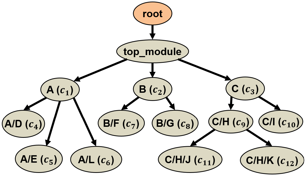
(a)

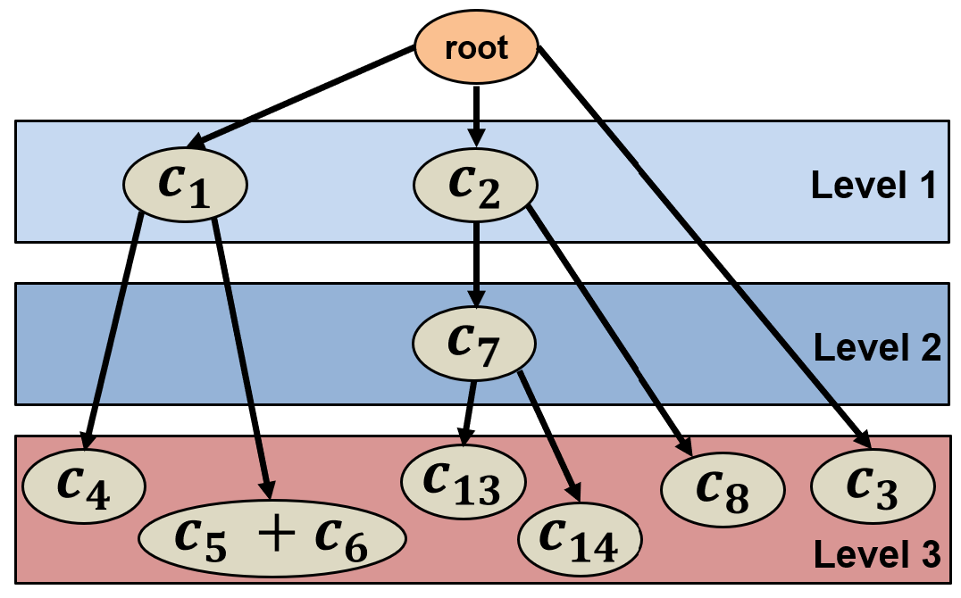
(b)

(c)

(d)

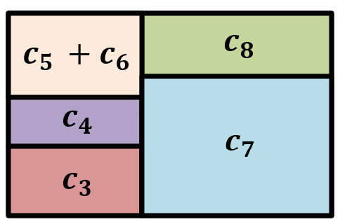
(e)

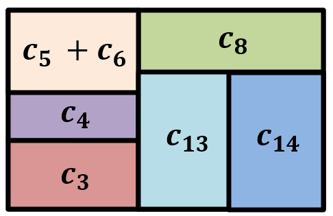
(f)

Figure 1: An illustrated example of a hierarchical floorplan scheme. (a) Logical hierarchy $T_{L}$. (b) Physical hierarchy $T_{P}$. In this example, the logical module $C$ is small and contains a limited number of instances. As a result, $c_{3}$ is classified as a leaf cluster. Any cluster within $c_{3}$ ($c_{9}$, $c_{10}$, $c_{11}$ and $c_{12}$) is not included in the final $T_{P}$. (c) Placed clusters in $T_{P}$ after visiting $root$ cluster. (d) Placed clusters in $T_{P}$ after visiting $c_{1}$ cluster. (e) Placed clusters in $T_{P}$ after visiting $c_{2}$ cluster. (f) Placed clusters in $T_{P}$ after visiting $c_{7}$ cluster, where $c_{7}$ is dissolved into $c_{13}$ and $c_{14}$. The placement of clusters is done in a pre-order DFS (depth-first search) manner.

• The logical hierarchy ($T_{L}$) is the original RTL hierarchy. Figure 1(a) shows an example of logical hierarchy $T_{L}$. Each node in $T_{L}$ represents a logical module in the netlist.

• The physical hierarchy ($T_{P}$) is the result of autoclustering and defines the physical clusters. The physical hierarchy can have multiple levels and is not necessarily balanced. Figure 1(b) shows an example of the physical hierarchy $T_{P}$.

• A physical cluster ($c$) is a module in the physical hierarchy. It can contain other physical clusters. In Figure 1(b), $c_{1},c_{2},{\color[rgb]{0,0,0}c_{3}},c_{4},c_{5}+c_{6},c_{7},c_{8},c_{13},c_{14}$ are the physical clusters. The top level of the design is the root physical cluster.

• A macro is a hard IP block, such as an SRAM block, which is predesigned and has a fixed layout. When placing a macro, we can change its location and orientation (typically, by mirroring and $180\text{\,}\mathrm{\SIUnitSymbolDegree}$ rotation, since the orientation of poly gates cannot be changed) but we cannot change anything inside it.

• A standard-cell cluster is a physical cluster that contains only standard cells.

• A macro cluster is a physical cluster that contains only macros.

• A mixed cluster is a physical cluster that contains both macros and standard cells.

• A leaf cluster is a standard-cell cluster or a macro cluster that does not have any children in the physical hierarchy $T_{P}$. In Figure 1(b), $c_{3}$, $c_{4}$, $c_{5}+c_{6}$, $c_{8}$, $c_{13}$ and $c_{14}$ are the leaf clusters.

• A bundled pin is the physical abstraction of a group of pins within the same boundary. All the pins belonging to a given bundled pin have the same physical location as the bundled pin.

Hier-RTLMP is built on top of the open-source OpenROAD infrastructure [26, 49] and works with the components within the OpenROAD flow, as shown in Figure 2. Our previous work, RTL-MP [51], partitions the top-level design into a set of leaf clusters, resulting in a single level of physical hierarchy. A known weakness of RTL-MP is that the single level of hierarchy makes it very difficult to generate decent macro placements for large, complex designs with hundreds of macros. By contrast, Hier-RTLMP’s multilevel physical hierarchy framework effectively scales the complexity of design blocks that can be handled, and incorporates tiling of macro groups along the periphery of physical clusters so as to honor the dataflow and produce a top-level floorplan with macros in the core area as needed.

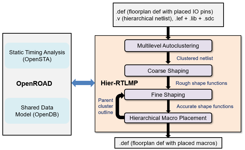
Figure 2: Hier-RTLMP flow.

The fundamental idea of Hier-RTLMP is that we first create a multilevel physical hierarchy, then shape and place the clusters in the physical hierarchy, one level at a time in a pre-order depth-first search manner. An overview of our Hier-RTLMP algorithm is presented in Algorithm 1. The input is a synthesized hierarchical gate-level netlist and a floorplan .def file that contains the block outline (width $canvas.width$ and height $canvas.height$), fixed IO pin or pad locations, along with macros that have been placed beforehand, if applicable. The output is a floorplan .def file that has legal macro placements for macros and region constraints for standard-cell clusters. Hier-RTLMP first converts the logical hierarchy $T_{L}$ of the netlist into a physical hierarchy $T_{P}$ (Section IV). Then, Hier-RTLMP determines the allowable shape functions for each of the clusters in a two-phase bottom-up and top-down manner (Section V). Finally, Hier-RTLMP works top-down from the root physical cluster in a pre-order depth-first search manner, and shapes and places the child clusters (Section VI).

Input: Hierarchical netlist $N$, Placed IO pins (or PAD)

   block outline ($canvas.width$, $canvas.height$)

Output: High-quality floorplan $F_{N}$ with fixed macro placements

1 initialize the floorplan $F_{N}$ with $canvas.width$ and $canvas.height$

2 update the positions of placed IO pins in $F_{N}$

3 convert the logical hierarchy $T_{L}$ of $N$ to the physical hierarchy $T_{P}$ (Section IV)

4 calculate the rough shape functions for each cluster in a bottom-up manner (Section V)

5 $c_{p}\leftarrow$ root cluster in $T_{P}$

6 $clusters\leftarrow c_{p}.GetChildren()$

7 adjust the possible shape functions for $clusters$ based on the outline of $c_{p}$ (Section V)

8 place $clusters$ within the outline of cluster $c_{p}$ (Section VI)

9 update the positions of $clusters$ in $F_{N}$

10 for leaf cluster $c_{f}\in clusters$ do

11       place the macros in leaf macro cluster $c_{f}$ (Section VI)

12      

13 end for

14for cluster $c\in c_{p}.GetChildren()$ do

15       $c_{p}\leftarrow c$; repeat Lines 5-15

16 end for

17return $F_{N}$

Algorithm 1 Hier-RTLMP

IV MULTILEVEL AUTOCLUSTERING

In this section, we describe the multilevel autoclustering approach. Subsection IV-A gives an overview, and Subsection IV-B provides a detailed explanation of how we perform autoclustering at each level.

IV-A Overview and Algorithm

In today’s design flows, expert human designers utilize clustering as an essential pre-processing step for macro placement. In this step the structural netlist representation of the design is converted to a clustered netlist in which the nodes are clusters and nets are bundled connections between the clusters. The clustering step is typically done by users interactively and in a top-down manner, by analyzing logical hierarchy, dataflow, connections between macros, IO pins, and critical timing paths [48]. Such analysis helps the user to understand the structure of the design and the dataflow, which provides insights into the ideal locations of the various clusters and macros. While it is useful for users to perform clustering manually and understand the physical implications of the design, it is also important to have an autoclustering engine that can fully and automatically generate meaningful clusters. This is especially true for designs produced by automatic RTL generators for ML applications; these can have complex RTL structures with long, inscrutable auto-generated module names. We therefore perform autoclustering based on the logical hierarchy of the design, connection signatures of clusters, and timing hops or indirect connections between macros and IO pins as outlined in RTL-MP [51] – and extend this to create a multilevel physical hierarchy.

The multilevel autoclustering engine in Hier-RTLMP extends the autoclustering engine in RTL-MP [51] to support multiple levels of physical hierarchy. It is essential for handling very large RTL blocks with multiple hundreds of macros. Moreover, the intermediate levels of physical hierarchy help preserve the global dataflow and allow for the placement of macros within the core of the floorplan. The multilevel autoclustering engine first converts logical hierarchy $T_{L}$ to physical hierarchy $T_{P}$ through a one-to-one mapping, i.e., transforming each logical module into a physical cluster directly. It then decides which clusters to merge and which clusters to dissolve level by level. Conceptually, peer clusters are merged if their individual sizes are below the minimum size threshold for the current level and if they have similar connection patterns to other clusters. A cluster is dissolved into its child clusters if its size is greater than the maximum size threshold for the current level.

In contrast to fully following the logical hierarchy, the operations of merging small peer clusters and dissolving large clusters enable us to extract the dataflow and functionality of the RTL. For example, some designs may have all the macros in a single logical module, even if these macros have completely different functionalities and connect to different standard-cell logical modules. Other designs could have the contents of a bus fabric, which connect to different sections of the block, in the same module of the logical hierarchy. In both these cases, it is obvious that fully following the logical hierarchy to create physical clusters will lead to suboptimal results from both the timing and congestion perspectives. However, the operations of merging and dissolving enable the multilevel autoclustering engine in Hier-RTLMP to effectively handle such scenarios from a physical floorplanning perspective.

Input: Hierarchical netlist $N$, Placed IO pins, Maximum depth of the physical hierarchy tree $num\_level$

Output: Physical hierarchy $T_{P}$ (depth $\leq num\_level$)

1 construct the logical hierarchy $T_{L}$ by traversing $N$

2 convert $T_{L}$ to the physical hierarchy $T_{P}$ by mapping each logical module in $T_{L}$ to a physical cluster $T_{P}$

3 divide each block boundary into $num\_segment$ segments and create a bundled pin for each segment to represent the preplaced IO pins (pads) lying on that segment

4 model each bundled pin as a child cluster of root cluster $root$ of $T_{P}$

5 $c_{p}\leftarrow root$ ; $level\_id\leftarrow 1$

6 while $level\_id<=num\_level$ and $level\_id>0$ do

7       single-level autoclustering($c_{p}$, $level\_id$) (Section IV-B)

8       for each child cluster $c$ of $c_{p}$ do

9             $c_{p}\leftarrow c$ ; $level\_id\leftarrow level\_id+1$

10             repeat the while loop [Lines 6-13]

11            

12       end for

13      $level\_id\leftarrow level\_id-1$

14      

15 end while

16 for each leaf cluster that is a mixed cluster, break it into a standard-cell cluster and a macro cluster

17 for each leaf cluster that is a macro cluster, mark its macros as single-macro macro clusters and group them based on connection signature. Then, for each newly formed macro cluster with macros of different sizes, break it down and group its macros based on their sizes

18 update connections between clusters by adding virtual connections between macro clusters and corresponding standard-cell clusters

19 update connections between clusters by adding virtual connections between clusters based on information flow and number of (latch) hops

return physical hierarchy $T_{P}$

Algorithm 2 Multilevel Autoclustering

The algorithm for multilevel autoclustering is shown in Algorithm 2. The entire autoclustering algorithm can be divided into the following steps.

Step 1: [Lines 1-2] We create the logical hierarchy $T_{L}$ by traversing the hierarchical netlist in a pre-order depth-first search manner. We then transform the logical hierarchy $T_{L}$ to the physical hierarchy $T_{P}$ based on a one-to-one mapping of each logical module to a physical cluster, i.e., $T_{P}$ = $T_{L}$. This one-to-one mapping between logical modules and physical clusters allows us to follow the logical hierarchy during the process of dissolving and merging physical clusters at each level. In the example of Figure 1(a), each logical module is mapped to a physical cluster directly, such as B/G to $c_{8}$ and C/H/J to $c_{11}$.

Step 2: [Lines 3-4] We create bundled pins by dividing each boundary edge evenly into $num\_segment$ segments, and assigning each bundled pin to the center of its corresponding segment (Section VII discusses the effect of $num\_segment$). Each bundled pin is treated as a physical cluster without physical area, and is added as a child cluster of the root node in the physical hierarchy $T_{P}$. A design may have thousands of IO pins. The bundled pin model can reduce the connection complexity significantly, while preserving the connections between clusters and IO pins and the affinity of clusters to related segments of boundaries in the floorplan.

Step 3: [Lines 5-13] We transform the physical hierarchy $T_{P}$ in a pre-order depth-first search manner. At each level, we create current-level clusters by breaking down the clusters from the parent level based on the size thresholds (the number of standard cells and the number of macros in a cluster) of the current level (see Section IV-B for details). After this step, we have a physical hierarchy $T_{P}$ with a depth less than or equal to $num\_level$. In the example of Figure 1, after Steps 1-3, we convert the logical hierarchy $T_{L}$ in Figure 1(a) into the physical hierarchy $T_{P}$ ($num\_level$ = 3) in Figure 1(b).

Step 4: [Line 14] Each leaf cluster that is a mixed cluster, is broken into a standard-cell cluster and a macro cluster. Separating into standard-cell clusters and macro clusters makes it easier to calculate the shape function for all the clusters (Section V). We also add a virtual weighted connection between each macro cluster and its corresponding standard-cell cluster to bias the macro placer to place them together.

Step 5: [Line 15] For each macro cluster, we mark each of its macros as a single-macro macro cluster (that is, a macro cluster consisting of only one macro) and group these single-macro macro clusters based on connection signatures (Section IV-B). This re-grouping of macros ensures that macros that have (near-)identical physical connectivity to other clusters are grouped together irrespective of where their instantiations occur in the logical hierarchy. If a newly-formed macro cluster has macros with different footprints, we break it down and regroup macros within it based on the footprints of the macros, which ensures that all the macros in the same macro cluster have the same shape. Grouping macros based on identical footprints enables better tiling of macros in macro groups with less wasted whitespace, thereby achieving regular placement of macros.

Step 6: [Line 17] We add virtual connections between clusters to capture the timing criticality between the clusters and to handle multiple pipeline stages in timing connections between clusters. The physical distances between components on critical timing paths should be minimized to improve performance. One approach is to determine all the critical timing paths (e.g., having negative slack) and overlay them on clusters. This is time-consuming and unnecessary since delay and slack calculation are not accurate at the floorplan stage. In this work, we use an approach similar to that of [34, 35] and define virtual (indirect) connections as

where information_flow corresponds to connection bitwidth and num_hops is the length of the shortest path of registers between clusters. However, unlike the Dataflow_Affinity defined in [34, 35], we use a more aggressive decaying factor as in [23, 24] to capture the most important indirect connections. If the register distance ($num\_hops)$ between clusters is greater than $num\_hop\_thr$ (default = 4), then no virtual connection is added. Also, in most designs, IO pins are registered before connecting to macros. It is important to capture this affinity during macro placement to ensure that the macros are placed close to “connected” IO pins. By treating each bundled pin as a cluster without physical area, indirect connections from primary inputs and to primary outputs can also be taken into account. As shown in Figure 3, in contrast to RTL-MP [51] which ignores the indirect connections between standard-cell clusters, Hier-RTLMP considers the indirect connections for all types of clusters (standard-cell clusters, macro clusters, mixed clusters and IOs), thus capturing the timing-critical paths more effectively. To more easily stop the calculation of indirect connections when the $num\_hops$ is larger than $num\_hop\_thr$, we start with all the macros and IO pins, and traverse the sequential graph in a breath-first search manner. Here we cannot use the topological order because the sequential graph of the netlist may contain cycles. Here, vertices of the sequential graph consist of all the flip-flops, macros and IO pins, and each edge in the sequential graph represents a directed combinational path, i.e., sequential adjacency in the netlist.

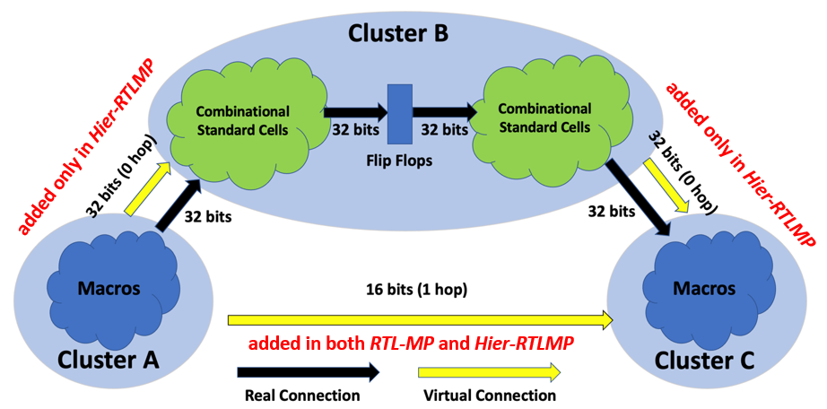
Figure 3: Virtual connections between clusters. Black arrows represent real connections and yellow arrows represent virtual connections. The virtual connections represented by yellow arrows can help capture critical timing paths between Clusters A, B and C. In RTL-MP, there is a virtual connection only between macro cluster A and macro cluster C. In Hier-RTLMP, the virtual connections between all the clusters are captured.

IV-B Single-level Autoclustering

At each level of the autoclustering process, we first create current-level clusters by breaking down the clusters from the parent level based on the size threshold of the current level, then merge small peer clusters and dissolve large clusters through traversing the logical hierarchy. We define four parameters related to the size threshold as described in [51]: max_num_inst and min_num_inst, the maximum and minimum number of standard-cell instances in a cluster; and max_num_macro and min_num_macro, the maximum and minimum number of macros in a cluster. The Hier-RTLMP flow takes $num\_level$ (the maximum depth of physical hierarchy tree) and $level\_ratio$ (the ratio of size threshold between the current level and its parent level) as inputs. Then the size threshold of each level decays exponentially as the $level\_id$ increases. For example, $max\_num\_inst$ of level $level\_id$ is the total number of instances of the design divided by $level\_ratio^{level\_id}$.

After determining the size threshold for the current level, we can create current-level clusters by breaking down the parent clusters from the upper level. Since we have created our physical hierarchy $T_{P}$ through a one-to-one mapping of each logical module to a physical cluster (Algorithm 2), we can further merge small peer clusters and dissolve large clusters through traversing the logical hierarchy.

In the example of Figure 1, logical modules $A$, $B$, $C$, $A/D$, $A/E$, $A/L$, $B/F$ and $B/G$ in logical hierarchy $T_{L}$ respectively correspond to physical clusters $c_{1}$, $c_{2}$, $c_{3}$, $c_{4}$, $c_{5}$, $c_{6}$, $c_{7}$ and $c_{8}$ in physical hierarchy $T_{P}$. Here, cluster $c_{7}$ which corresponds to logical module $B/G$ is between the minimum, maximum size thresholds of level $2$, but larger than the maximum size threshold of level $3$. Hence $c_{7}$ is dissolved into clusters $c_{13}$ and $c_{14}$ using a partitioner. Clusters $c_{5}$ and $c_{6}$ which correspond to logical modules $A/E$ and $A/L$ are smaller than the minimum size threshold of level $3$. Hence $c_{5}$ and $c_{6}$ are merged into cluster $c_{5}+c_{6}$. Cluster $c_{3}$ which corresponds to logical module $C$ is within the size thresholds of level $3$. Hence, $c_{3}$ is a leaf cluster, and any cluster within $c_{3}$ ($c_{9}$, $c_{10}$, $c_{11}$ and $c_{12}$) is not included in the final $T_{P}$.

Input: Parent cluster $c_{p}$, Level id $level\_id$

1 determine size thresholds for current level

2 $children\leftarrow c_{p}.GetChildren()$

3 initialize an empty cluster list $new\_children$

4 if $children.size()==0$ then

5       $new\_children\leftarrow$ recursively call TritonPart to bipartition $c_{p}$ until the number of standard cells in each child cluster is less than $max\_num\_inst$

6 else

7       initialize an empty cluster list $candidate\_clusters$

8       for each cluster $c\in children$ do

9             if $c.num\_macro>max\_num\_macro$ or $c.num\_std\_cell>max\_num\_inst$  then

10                   $c_{p}\leftarrow c$; repeat Lines 2-18

11             else if $c.num\_macro<min\_num\_macro$ and $c.num\_std\_cell<min\_num\_inst$ then

12                   $candidate\_clusters.push\_back(c)$

13                  

14             else

15                   $new\_children.push\_back(c)$

16                  

17             end if

18            

19       end for

20      merge clusters in $candidate\_clusters$ based on connection signature

21      

22 end if

23$c_{p}.SetChildren(new\_children)$

Algorithm 3 Single-level Autoclustering

The detailed algorithm is presented in Algorithm 3 and the entire single-level autoclustering algorithm can be divided into the following steps.

Step 1: [Line 1] Determine the size thresholds for the current level, including $max\_num\_inst$, $min\_num\_inst$, $max\_num\_macro$ and $min\_num\_macro$.

Step 2: [Lines 4-5] If the parent cluster $c_{p}$ is a leaf cluster, and its size is larger than the threshold for the current level, we recursively call the open-source partitioner TritonPart [49] in min-cut mode to bipartition the cluster $c_{p}$ into child clusters that meet the size threshold (number of standard cells) for the current level. Each instance in cluster $c_{p}$ is treated as a vertex. Here, we do not need to consider the size threshold for number of macros because the macros will be grouped separately later [Algorithm 2 Line 15].

Step 3: [Lines 6-18] We handle each child cluster of parent cluster $c_{p}$ based on the size thresholds in a pre-order depth-first search manner. During this step, we break down each large cluster (number of macros $>max\_num\_macro$ or number of standard cells $>max\_num\_inst$) according to the logical hierarchy, and merge the small clusters (number of macros $<min\_num\_macro$ and number of standard cells $<min\_num\_inst$) based on connection signature. Here, the connection signature is the connection topology of a cluster with respect to the other clusters in the physical hierarchy $T_{P}$, which calibrates the connection similarity of clusters. More specifically, for a cluster $c$ and a threshold $\epsilon_{net}$, the connection signature $conn\_hash(c)$ of cluster $c$ with respect to clusters $\{c_{1},c_{2},...,c_{n}\}$ (termed as reference clusters) is a vector of size $n$ such that

$$conn\_hash(c)[i]=\begin{cases}1\quad&\text{if the number of nets between}\\ &\text{$c$ and $c_{i}$ is larger than $\epsilon_{net}$},\\ 0\quad&\text{otherwise}\\ \end{cases}$$

The threshold $\epsilon_{net}$ (default $=50$) is introduced to remove spurious effects of common global nets such as scan or reset signals. The intuition behind merging clusters with the same connection signature is that clusters with similar connection patterns would want to stay together in the floorplan. Moreover, the small clusters being merged satisfy the following two criteria: (i) they belong to the same logical module; and (ii) they have similar bus structures, i.e., the number of nets connecting to any reference cluster should be similar.

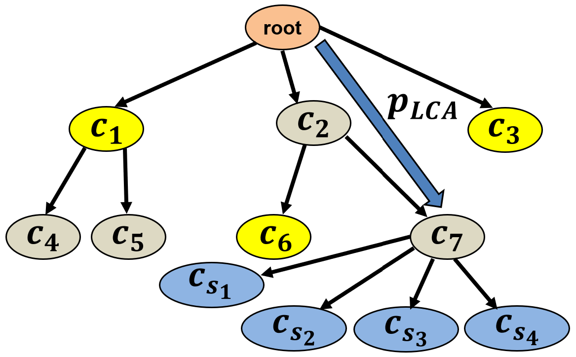
(a)

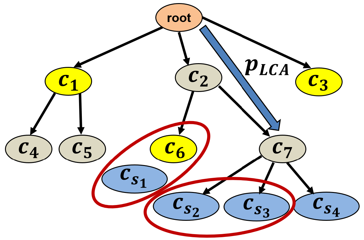
(b)

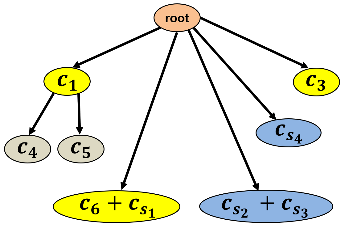
(c)

Figure 4: An example of merging clusters based on connection signature. $\{c_{s_{1}},c_{s_{2}},c_{s_{3}},c_{s_{4}}\}$ are the candidate clusters to be merged. $c_{7}$ is the least common ancestor and $p_{LCA}=\{root,c_{2},c_{7}\}$ the shortest path between root node $T_{P}$ and $c_{7}$. $\{c_{1},c_{3},c_{6}\}$ are the reference clusters. Notably, cluster $c_{s1}$ only connects to cluster $c_{6}$, and cluster $c_{s2}$ and cluster $c_{s3}$ have the same connection signature. Thus, $c_{s1}$ and $c_{6}$ will be merged into one cluster $c_{s1}+c_{6}$, and $c_{s2}$ and $c_{s3}$ will be merged into one cluster $c_{s2}+c_{s3}$, as indicated by red ellipses in (b). Shown in the figure: physical hierarchy $T_{P}$ (a) before merging; (b) during merging; and (c) after merging.

Input: Candidate clusters $\{c_{s_{1}},...,c_{s_{k}}\}$

1 find the least common ancestor $v_{LCA}$ of $\{c_{s_{1}},...,c_{s_{k}}\}$ in tree $T_{P}$

2 find the shortest path $p_{LCA}$ between root node of $T_{P}$ and $v_{LCA}$

3 $reference\_clusters=\{\}$

4 for each node $v\in p_{LCA}$ do

5       if $v{\color[rgb]{0,0,0}\neq}v_{LCA}$ then

6             for each node $u\in v.children()$ do

7                   if $u\not\in p_{LCA}$ then

8                         $reference\_clusters.append(u)$

9                        

10                   end if

11                  

12             end for

13            

14       end if

15      

16 end for

17calculate the connection signatures of $\{c_{s_{1}},...,c_{s_{k}}\}$ with respect to $reference\_clusters$

18 for each cluster $c\in\{c_{s_{1}},...,c_{s_{k}}\}$  do

19       if $c$ connects to only one of the reference clusters then

20             merge $c$ with that reference cluster

21       end if

22      

23 end for

24merge remaining clusters in $\{c_{s_{1}},...,c_{s_{k}}\}$ with the same connection signature

25 update tree $T_{P}$

Algorithm 4 Merge Clusters Based on Connection Signature

In contrast to RTL-MP [51], we extend the calculation of connection signature to a multilevel context. Details are given in Algorithm 4. The entire process is illustrated with the example shown in Figure 4. In this example, $\{c_{s_{1}},c_{s_{2}},c_{s_{3}},c_{s_{4}}\}$ are the candidate clusters to be merged. First, we find the least common ancestor of $\{c_{s_{1}},c_{s_{2}},c_{s_{3}},c_{s_{4}}\}$, i.e., $c_{7}$ [Line 1]. Second, we determine the shortest path $P_{LCA}={root,c_{2},c_{7}}$ between root node and $c_{7}$ [Line 2]. Third, we traverse $P_{LCA}$ and identify all the reference clusters $\{c_{1},c_{3},c_{6}\}$ [Lines 3-12]. We then calculate the connection signatures of $\{c_{s_{1}},c_{s_{2}},c_{s_{3}},c_{s_{4}}\}$ with respect to $\{c_{1},c_{3},c_{6}\}$ [Line 13]. Fourth, if a candidate cluster connects to only one of the reference clusters, we merge the candidate cluster with that reference cluster directly [Lines 14-18]. As shown in the figure, if cluster $c_{s1}$ only connects to cluster $c_{6}$, we will merge $c_{s1}$ with $c_{6}$. Finally, we merge remaining candidate clusters having the same connection signature and update the physical hierarchy tree $T_{P}$ [Lines 19-20]. For example, if cluster $c_{s2}$ and $c_{s3}$ have the same connection signature, we will merge $c_{s2}$ and $c_{s3}$. The final physical hierarchy is shown in Figure 4(c). As shown in the figure, the final physical hierarchy is different from the original logical hierarchy: (i) there are physical clusters in the physical hierarchy that correspond to multiple logical modules in the logic hierarchy; and (ii) the physical hierarchy tree $T_{p}$ is unbalanced and has a different structure from the logical hierarchy.

V SHAPE FUNCTIONS FOR CLUSTERS

Shape function calculation [19] determines the allowable rectangular shapes for each cluster. In RTL-MP [51], the physical hierarchy has a single level, and all clusters are leaf clusters; shape functions are continuous for standard-cell clusters and discrete for macro clusters. By contrast, in Hier-RTLMP, shape functions are calculated for all the intermediate levels of the physical hierarchy, leading up to the root, using a two-step process. First, shape functions are initially calculated bottom-up from leaf clusters. Second, once the shape functions for all clusters in the physical hierarchy have been calculated, they are further refined before the top-down macro placement of the clusters, starting from the root cluster. Conceptually, during bottom-up determination of the shape functions, we still do not know the outline nor the IO pin locations for the parent cluster. During the top-down macro placement of the physical clusters, starting from the root cluster (i.e., the top-level design), both the outline and the IO pin locations are fixed. Hence, the shape functions of child clusters can be further refined to better accommodate the parent cluster’s outline and IO pin locations. This enables improved convergence and outcomes (runtime and QoR) during the macro placement of a given parent cluster. The remainder of this section gives details of how cluster shape functions are determined.

Recall from Section III above that there are standard-cell, macro, and mixed types of clusters.

• A standard-cell cluster (containing only standard cells) has fixed area and continuous aspect ratio within given lower and upper bounds. As shown in Figure 5, the shape function of a standard-cell cluster is a continuous curve.

• A macro cluster (containing only macros) can have different areas and discrete aspect ratios. As shown in Figure 5, the shape function of a macro cluster is a set of discrete points.

• A mixed cluster (containing both macros and standard cells) has fixed area and piecewise-continuous aspect ratios. As shown in Figure 5, the shape function of a mixed cluster (red trace) is a piecewise-continuous curve.

Figure 5: Example shape curves for standard-cell, macro, and mixed cluster types, during coarse (stage 1) and fine (stage 2) shaping. The blue line represents the shape curve of a standard-cell cluster during fine (stage 2) shaping; the two red dots and two segments of red lines respectively represent the shape curves of a mixed cluster during coarse (stage 1) and fine (stage 2) shaping; and the two black dots represent the shape curve of a macro cluster during coarse (stage 1) shaping.

We calculate the shape functions of clusters in a “$\Lambda$-shaped” multilevel manner, i.e., following the traditional multilevel paradigm. This enables Hier-RTLMP to dynamically adjust the possible shapes for each cluster, based on the placement (Section VI). The overall shape function calculation can be divided into two stages, which respectively perform coarse shaping and fine shaping, as follows.

Coarse Shaping (Stage 1). During coarse shaping, we determine the rough shape function for each cluster in a bottom-up manner, which means the shapes of a cluster are based on the tilings of all its child clusters. This method of bottom-up calculation for shape functions guarantees that the determined shape of a macro or mixed cluster is always large enough to accommodate the tilings of all the included macros. Coarse shaping consists of the following steps. First, the shape of a standard-cell cluster is constrained by a user-specified parameter $min\_ar$ (default value = 0.33), i.e., the aspect ratio of a standard-cell cluster is in the range $[min\_ar,\frac{1.0}{min\_ar}]$. Second, for the shape function of a macro cluster, we use Simulated Annealing to calculate possible macro tilings, which have minimum area and can fit into the floorplan. Third, for the shape function of a mixed cluster, we ignore the area of standard cells, and use Simulated Annealing to calculate possible tilings of its child clusters. As applied in this phase, the Sequence Pair-based annealing supports four solution perturbation (move) operators with respective probabilities 0.3, 0.3, 0.3 and 0.1:

• Op1: Swap two clusters in the first sequence;

• Op2: Swap two clusters in the second sequence;

• Op3: Swap two clusters in each of both sequences; and

• Op4: Change the shape of a cluster by randomly picking one shape from its available shapes.

The details of Simulated Annealing are as follows: the number of moves per iteration is 500; the total number of iteration is 200; the initial acceptance probability is 0.9; and the minimum temperature is $1e^{10}$. Here we also force the aspect ratio of a mixed cluster to be within the range $[min\_ar,\frac{1.0}{min\_ar}]$ if there are multiple available possible tilings. As shown in Figure  5, after coarse shaping we know the shape functions for macro clusters, and the discrete approximation of the shape functions for mixed clusters, for the entire physical hierarchy.

Fine Shaping (Stage 2). Fine shaping is done in a top-down manner, starting from the root cluster, and before the macro placement of each given cluster to dynamically adjust the possible shapes of each of the child clusters. At this stage, we refine the possible shapes of each cluster based on the fixed outline and location of its parent cluster. For the root cluster, which is the top-level block, the fixed outline and the IO pin locations are the input constraints, usually derived from the starting floorplan .def file. Details are given in Algorithm 5. First, we remove the area occupied by placement blockages from the available area of parent cluster $c_{p}$ [Lines 1-2]. Second, for each macro cluster, we abandon the shapes that cannot fit into the outline of parent cluster $c_{p}$ [Lines 4-7]. Third, for each mixed cluster, we inflate the area of standard cells based on the target utilization $util$, then convert the discrete shapes into continuous shapes (see the example in Figure 5) by adding the area of standard cells [Lines 8-21]. Fourth, we check if there is enough empty space for standard-cell clusters [Lines 26-28]. Finally, we inflate the area of standard cells based on target dead space $t\_dead\_space$. Here we ignore the area of tiny clusters which only have tens of standard cells [Lines 29-38]. The target dead space controls the amount of whitespace in the floorplan.

Conceptually, the larger the $t\_dead\_space$ and $util$ (the smaller the area of mixed clusters and standard-cell clusters), the easier it is to generate a valid macro placement that optimizes wirelength, but this may cause significant routing issues. In order to avoid high congestion, physical clusters with higher macro density usually require lower utilization. Thus, in contrast to all previous works, we dynamically inflate the area of standard cells in mixed clusters and standard-cell clusters based on target utilization $util$ and target dead space $t\_dead\_space$, respectively. Furthermore, since it is difficult to find universal values of target utilization $util$ and target dead space $t\_dead\_space$ parameters that succeed for all designs, we sweep these two parameters within given user-specified computing resource and runtime constraints, and pick the best floorplan obtained from the given budget of trials. More specifically, for each target utilization $util$, we sweep the target dead space $t\_dead\_space$ parameter. The sweeping stops when the current shape functions for clusters result in a valid placement of clusters; in our experiments, this occurs within 10 to 30 trials. The runtime reported in Section VII includes the total runtime of all the trials. The runtime analysis in Section VII also suggests that the runtime overhead of sweeping the target dead space $t\_dead\_space$ and target utilization $util$ is not significant.

Input: Physical hierarchy tree $T_{P}$, Placed parent cluster $c_{p}$,

   Target utilization $util$,

   Target dead space $t\_dead\_space$,

   Minimum aspect ratio $min\_ar$

1 $avail\_area\leftarrow c_{p}.GetOutlineArea()$

2 $avail\_area\mathrel{{-}{=}}$ area occupied by placement blockages

3 for cluster $c$ $\in$ $c_{p}.GetChildren()$ do

4       if $c$ is a macro cluster then

5             abandon the shapes which cannot fit into $c_{p}$

6             $avail\_area\mathrel{{-}{=}}c.GetArea()$

7            

8       end if

9      if $c$ is a mixed cluster then

10             abandon the shapes which cannot fit into $c_{p}$

11             $shapes\leftarrow c.GetShapes()$

12             $area\leftarrow$ the minimum area of possible shapes

13             $area\leftarrow area+c.GetStdCellArea()/util$

14             initialize an empty list $aspect\_ratios$

15             for each $shape$ in $shapes$ do

16                   $ar=[\frac{shape.height}{area/shape.height},\frac{area/shape.width}{shape.width}]$

17                   $aspect\_ratios.push\_back(ar)$

18                  

19             end for

20            $c.SetArea(area)$

21             $c.SetAspectRatios(aspect\_ratios)$

22             $avail\_area\mathrel{{-}{=}}area$

23            

24       end if

25      

26 end for

27if $c_{p}.GetStdCellArea()==0.0$ then

28       return true

29      

30 end if

31if $avail\_area\leq 0.0$ then

32       return false

33      

34 end if

35$inflat\_ratio=\frac{c_{p}.GetStdCellArea()}{avail\_area*(1-t\_dead\_space)}$

36 for each child standard-cell cluster $c$ of $c_{p}$ do

37       if $c$ is a tiny cluster then

38             $c.SetArea(0.0)$

39            

40       end if

41      else

42             $c.SetArea(\frac{c.GetArea()}{inflat\_ratio})$

43             $c.SetAspectRatios([min\_ar,\frac{1.0}{min\_ar}])$

44            

45       end if

46      

47 end for

48return true

Algorithm 5 Fine Shaping

VI HIERARCHICAL MACRO PLACEMENT

In this section, we describe our approach to top-down hierarchical macro placement. Subsection VI-A describes how we place and shape the physical clusters, one level at a time, in a pre-order depth-first search manner. Subsection VI-B describes how we determine the location and orientation of macros in each leaf macro cluster.

VI-A Placement of Clusters

We shape and place the physical clusters, one level at a time, in a pre-order depth-first search manner starting from the root cluster. Before the placement of clusters at each level, we first determine the shape functions for all clusters based on the outline and location of the parent cluster (Fine Shaping in Section V). For example, in Figure 1, before we place and shape clusters $c_{7}$ and $c_{8}$, we adjust the shape functions of $c_{7}$ and $c_{8}$ based on the outline and location of their parent cluster $c_{2}$. We then calculate the connections between clusters, IO pins and other clusters of the parent level. The other clusters of the parent level are the reference clusters described in Section IV-B. The actual IO pins are modeled by the bundled pins along the block boundary, as described in Section IV. At the top level (i.e., root cluster of $T_{P}$), there are no other clusters of the parent level. Below the top level, i.e., when we are working on the physical clusters at intermediate levels of the physical hierarchy, the outlines and locations of clusters of the parent level have already been calculated, and behave like fixed terminals. For example, in Figure 1, when we place clusters $c_{13}$ and $c_{14}$, other clusters of the parent level ($c_{1}$, $c_{3}$ and $c_{8}$) behave like fixed terminals. In our implementation, we assume that the bundled pin of each cluster is at the center of the cluster. We use Sequence Pair [14] to represent a given (floorplanned) arrangement of clusters, and Simulated Annealing [27] to optimize a heuristic cost function. Further, we adopt “multi-start” scheme to improve the performance of Simulated Annealing and we set the number of threads to 10 in our experiments. As applied in this phase, the Sequence Pair-based annealing supports four solution perturbation (move) operators with respective probabilities 0.3, 0.3, 0.3 and 0.1:

• Op1: Swap two clusters in the first sequence;

• Op2: Swap two clusters in the second sequence;

• Op3: Swap two clusters in each of both sequences; and

• Op4: Resize a cluster. For standard-cell clusters and mixed clusters, we use the same resizing algorithm as in [6]; for macro clusters, we randomly pick one shape of its shapes.

To improve the QoR of the floorplan, we handle the following constraints as RTL-MP does.

• Fixed outline: All clusters should be placed within the fixed outline. At the top level (root cluster of the physical hierarchy $T_{P}$), the outline is the block boundary defined in the input .def file. Below the top level, for an intermediate level physical cluster, the outline is determined by the shape and location of its parent cluster.

• Peripheral bias: To take routing blockages (e.g., due to internal routing within macros) into account, leaf clusters with macros should be pushed to peripheries of the boundary. This simplifies the routing process by reducing congestion in the center region.

• Blockage: Instances including both macros and standard cells should not overlap with placement blockages. Since preplaced macros can be treated as placement blockages, our macro placer can also handle preplaced macros.

• Guidance: All clusters should be placed near specified regions if users provide such constraints. The cluster’s guidance is determined by the bounding box that encompasses the guidance for all constituent macros. We do not consider the guidance for macros or clusters during multilevel autoclustering.

• Notch avoidance: A decent floorplan should avoid dead space which cannot be used effectively by P&R tools.

• Pin access: Macros should be kept from blocking the access of IO pins.

In summary, the final cost function of our macro placer is

$$\begin{split}cost&=\alpha\times Area+\beta\times WL+\gamma\times p_{outline}\\ &+\zeta\times p_{bias}+\eta\times p_{blockage}\\ &+\theta\times p_{guidance}+\lambda\times p_{notch}\end{split}$$ (2)

where $Area$ is the area of the current floorplan, $WL$ is the wirelength (HPWL), $p_{outline}$ is the penalty for violating the fixed outline constraint, $p_{bias}$ is the penalty to promote macro peripheral bias, $p_{blockage}$ is the penalty for pin access and macro blockage, $p_{guidance}$ is the penalty for macro guidance, $p_{notch}$ is the penalty for notch regions, and $\alpha$, $\beta$, $\gamma$, $\zeta$, $\eta$, $\theta$ and $\lambda$ are the corresponding weights. $Area$, $WL$, $p_{outline}$, $p_{bias}$, $p_{blockage}$, $p_{guidance}$ and $p_{notch}$ are all normalized by the corresponding initial value. The default values of these weights are available in [62], and the effects of tuning these weights are studied in Section VII.

VI-B Placement of Macros

After the placement of clusters, we know the position and shape for each cluster. We next determine the location and orientation of macros in each leaf macro cluster, one macro cluster at a time. For a given macro cluster A, we extract the connections between macros in A and in other clusters. Here, other clusters behave like fixed terminals. We use Sequence Pair [14] to represent macro placement in A and Simulated Annealing [27] to optimize the cost function. We use four solution perturbation (move) operators in the annealing, with respective probabilities 0.3, 0.3, 0.3 and 0.1:

• Op1: Swap two macros in the first sequence;

• Op2: Swap two macros in the second sequence;

• Op3: Swap two macros in each of both sequences; and

• Op4: Flip all the macros.

The cost function used in this step is

$$cost=\alpha\times Area+\beta\times WL+\gamma\times p_{outline}+\theta\times p_{guidance}$$ (3)

where $Area$ is the area of the current macro packing, $WL$ is the wirelength (HPWL), $p_{outline}$ is the penalty for violating the fixed-outline constraint, $p_{guidance}$ is the penalty for macro guidance, and $\alpha,\beta$, $\gamma$ and $\theta$ are corresponding weights.

VII EXPERIMENTAL VALIDATION

Hier-RTLMP is implemented with approximately 12K lines of C++ with a Tcl command line interface on top of the OpenROAD [26, 49] infrastructure. We have validated our macro placer using multiple designs including Ariane [57], BlackParrot (Quad-Core) [58], MemPool Group [59], Tabla09 [52], Tabla01 [52] and Arm Cortex-A53 (CA53), in both open NanGate45 (NG45) and commercial GlobalFoundries 12nm (GF12) enablements. Tabla09 and Tabla01 are machine learning accelerators generated by an open-source machine learning hardware generator [52]. We use the bsg_fakeram [56] memory generator to generate SRAMs for NanGate45 enablement. The commercial GlobalFoundries 12nm enablement is a commercial foundry 12nm technology (13 metal layers) with cell library and memory generators from a leading IP provider. Table II summarizes information about our designs.

TABLE II: Benchmarks. The clock periods for testcases implemented in GF12 are not specified, to protect foundry IP. $Min\_AR$ and $Max\_AR$ respectively denote the minimum and maximum aspect ratios of macros within the testcase. Area Ratio refers to the ratio between the maximum and minimum areas of macros in the testcase.

Designs	Enablements	Macros	Std Cells	Clock Period	Utilization	Min_AR Max_AR	Area Ratio
Ariane	NG45	133	118K	1.3 ns	0.70	1.53 / 2.31	2.37
BlackParrot	NG45	220	769K	5.2 ns	0.69	0.61 / 3.24	14.14
CA53	GF12	25	445K	—–	0.73	0.90 / 4.80	8.83
Ariane	GF12	133	95K	—–	0.68	0.95 / 0.95	1.00
BlackParrot	GF12	196	827K	—–	0.75	1.38 / 4.54	3.96
Tabla09	GF12	368	245K	—–	0.75	0.88 / 3.38	11.74
Tabla01	GF12	760	431K	—–	0.75	1.55 / 3.38	18.52
MemPool	GF12	326	2529K	—–	0.62	1.35 / 3.77	2.79

To show the effectiveness of our macro placer, the following three scenarios are evaluated and compared.

• Comm: Macro placement is performed using a 2021 release of a state-of-the-art commercial P&R tool (unnamed due to EULA restrictions) with its latest macro placement option.

• RTL-MP: Macros are placed by our previous work, RTL-MP [51].

• Hier-RTLMP: Results are obtained using our new macro placer.

Our experiments use the following flow. (1) We first synthesize the design using a state-of-the-art commercial synthesis tool, preserving the logical hierarchy. (2) Next, we determine the core size of the testcase, and place all the IO pins according to the determined core size using a manually-developed script. The utilization for each testcase is presented in Table II. (3) Then, the macros are placed using different methods (Comm, RTL-MP and Hier-RTLMP). (4) Last, all standard cells are placed, and all nets are routed, using Cadence Innovus v21.1. Our scripts for power delivery network generation and standard-cell placement and routing are similar to those publicly visible in the MacroPlacement GitHub repository [50].

VII-A Comparison of Hier-RTLMP with Other Macro Placers

Table III and Table IV show the experiment results after completion of post-routing optimization (postRouteOpt) starting from different macro placers’ solutions on our testcases. All the macro placers are executed using their default parameter settings. The effect of parameter tuning is discussed in Section VII-C. Rows represent designs, enablements and macro placement flows; columns give metrics of number of standard cells, total routed wirelength, power, worst negative slack (WNS), total negative slack (TNS) and turnaround time for a single run. The metrics in GF12 are normalized to protect foundry IP: (i) standard-cell area is normalized to core area; (ii) wirelength and power are normalized to the Comm result; and (iii) timing metrics (WNS, TNS) are normalized to the clock period which we leave unspecified. In all experiments that we report, we allow Hier-RTLMP to sweep the target dead space $t\_dead\_space$ from 0.05 to 1.0 with step 0.05, and target utilization $util$ from 0.25 to 1.0 with step 0.1. To reduce the runtime of $t\_dead\_space$ and $util$ sweeping, we set the number of threads to 10.

As noted in Section V, the parameter sweep stops with the first valid placement of clusters (in practice, within 10 to 30 trials). The turnaround time for a single run reported includes the total runtime of all the trials (see Section VII-D for detailed runtime analysis). Hier-RTLMP outperforms the commercial macro placer and RTL-MP for almost all the testcases.

Compared to RTL-MP. Table III shows that Hier-RTLMP reduces runtime compared to RTL-MP by at least $13\times$. For CA53 (GF12), Hier-RTLMP generates worse results than RTL-MP. However, Hier-RTLMP can achieve similar TNS through applying autotuning enhancement (see Section VII-C). For Ariane (GF12), Hier-RTLMP generates better results than RTL-MP. The corresponding layouts of CA53 (GF12) and Ariane (GF12) are presented in Figure 6.

TABLE III: Metrics of Comm, RTL-MP and Hier-RTLMP for designs in commercial GF12 enablements. We highlight best values of timing metrics in blue bold font. Data points for GF12 are normalized.

Design (Enablement)								Macro Placer	Std Cell Area ($mm^{2}$)	WL ($m$)	Power ($mW$)	WNS (ps)	TNS (ns)	TAT ($min$)
CA53 (GF12)	Comm	0.166	1.00	1.00	-0.23	-277	68
	RTL-MP	0.167	1.04	1.01	-0.23	-145	71
	Hier-RTLMP	0.168	1.08	1.03	-0.26	-167	5
Ariane (GF12)	Comm	0.045	1.00	1.00	-0.17	-156	11
	RTL-MP	0.045	1.29	1.02	-0.13	-108	200
	Hier-RTLMP	0.045	1.21	1.01	-0.09	-63	9

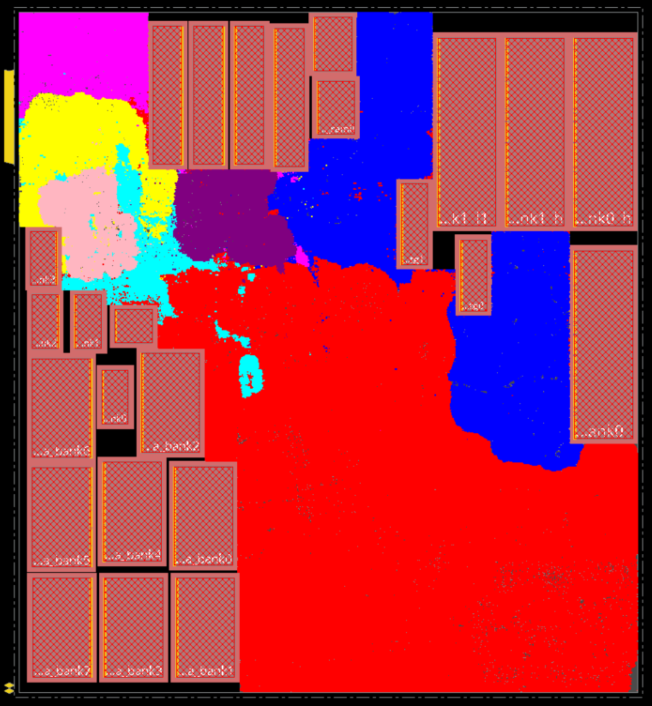
(a) CA53 (GF12) / Comm

(b) CA53 (GF12) / RTL-MP

(c) CA53 (GF12) / Hier-RTLMP

(d) Ariane (GF12) / Comm

(e) Ariane (GF12) / RTL-MP

(f) Ariane (GF12) / Hier-RTLMP

Figure 6: Macro placements generated by Comm, RTL-MP and Hier-RTLMP.

Compared to commercial macro placers. Table IV shows that Hier-RTLMP achieves much better timing in terms of WNS and TNS within similar or less runtime. Besides, Hier-RTLMP can identify the dataflow of design and place macros following the dataflow. For example, for the Tabla09 design, Figure 7(b) shows the layout for the macro placement generated by Hier-RTLMP and Figure 7(c) shows the placement for the child clusters of the root (top-level) cluster. At the root level of the physical hierarchy, five clusters are mixed clusters containing both macros and standard cells. There is one IO cluster containing memories ($mem$, yellow rectangle), and four functional units each of which is an individual mixed cluster ($PU0$ to $PU3$, red rectangles). The standard-cell clusters at the top level, which are “tiny clusters” (Section V), contain muxing logic that processes the IOs and interfaces with the four functional units. As can be seen from Figure 7(b), the placement follows the dataflow with the IO cluster close to the IOs and the standard-cell cluster in the middle of the four functional unit clusters. The black lines in Figure 7(c) show the bundled net connections. The Tabla01 design has a similar architecture as Tabla09, but with eight functional units ($PU0$ to $PU7$). The results are presented in Figure 7(d)-(f). The layouts for Mempool (GF12) are presented in Figure 7(g)-(h).

TABLE IV: Metrics of Comm and Hier-RTLMP for designs in open NG45 and commercial GF12 enablements. We highlight best values of timing metrics in blue bold font. Data points for GF12 are normalized.

Design (Enablement)								Macro Placer	Std Cell Area ($mm^{2}$)	WL ($m$)	Power ($mW$)	WNS ($ps$)	TNS ($ns$)	TAT ($min$)
Ariane (NG45)	Comm	0.247	4.35	835	-258	-629	4
	Hier-RTLMP	0.247	5.27	833	-97	-55	8
BlackParrot (NG45)	Comm	1.926	24.62	4461	-193	-2113	23
	Hier-RTLMP	1.924	28.73	4509	-100	-170	28
BlackParrot (GF12)	Comm	0.21	1.00	1.00	-0.10	-1147	118
	Hier-RTLMP	0.21	1.20	1.02	-0.08	-444	69
Tabla09 (GF12)	Comm	0.05	1.00	1.00	-0.52	-180	36
	Hier-RTLMP	0.05	0.89	0.95	-0.18	-74	37
Tabla01 (GF12)	Comm	0.06	1.00	1.00	-0.51	-125	40
	Hier-RTLMP	0.06	0.92	0.93	-0.04	0	105
MemPool (GF12)	Comm	0.34	1.00	1.00	-0.17	-1305	554
	Hier-RTLMP	0.34	1.12	1.05	-0.16	-1227	167

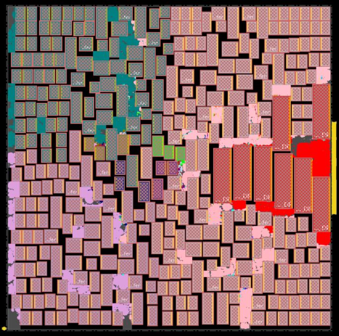
(a) Tabla09 (GF12) / Comm

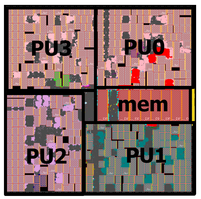
(b) Tabla09 (GF12) / Hier-RTLMP

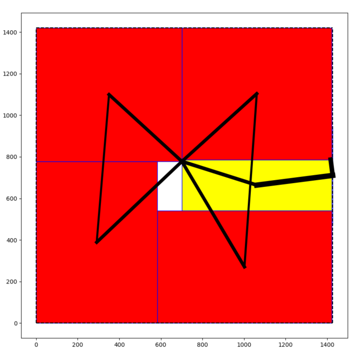
(c) Tabla09 (GF12) dataflow

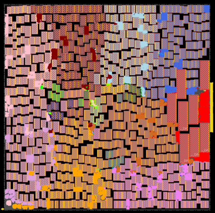
(d) Tabla01 (GF12) / Comm

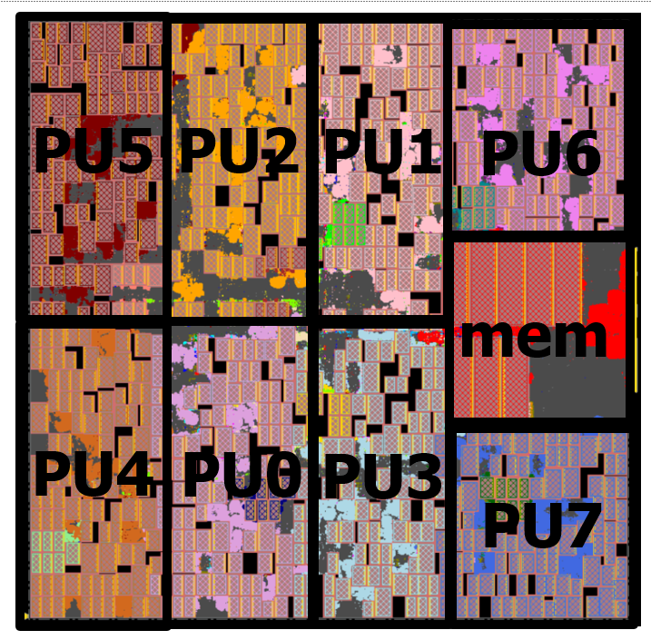
(e) Tabla01 (GF12) / Hier-RTLMP

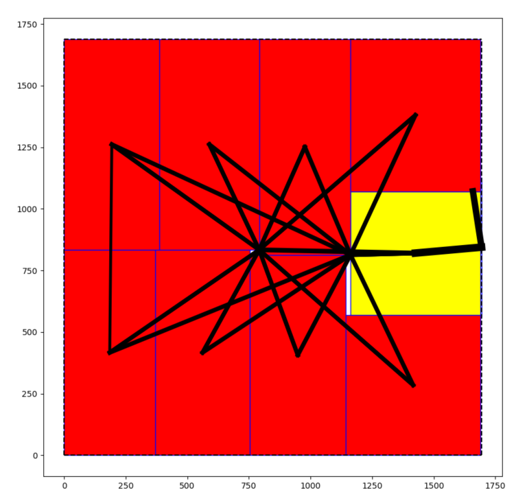
(f) Tabla01 (GF12) dataflow

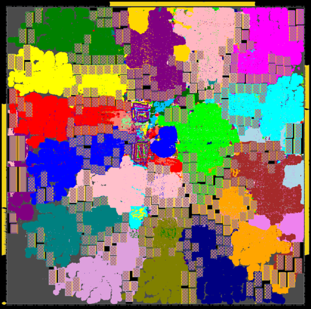
(g) MemPool (GF12) / Comm

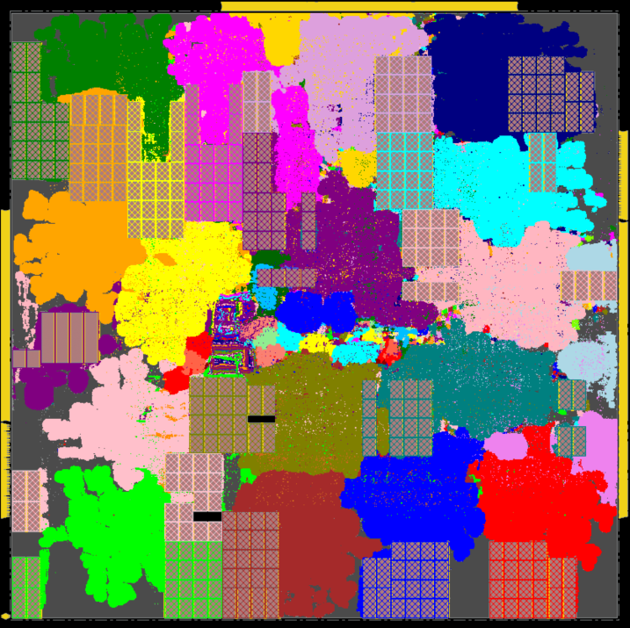
(h) MemPool (GF12) / Hier-RTLMP

Figure 7: Macro placements generated by Comm and Hier-RTLMP.

VII-B Effect of Timing Awareness

Hier-RTLMP captures the multiple stages of timing paths between clusters through adding virtual connections between clusters (Section IV-A). Figure 8 shows the effect of varying the threshold of $num\_hops$ (the length of the shortest path of registers between paths) in Equation (1), which affects the computation of timing-related virtual connections between clusters. Here we use Ariane (NG45), CA53 (GF12) and BlackParrot (GF12) as our testcases, and sweep $num\_hops\_thr$ across values {0, 1, 2, 3, 4, 5}, where $num\_hops\_thr=0$ means that no multiple stages of timing paths are considered. We can see that $num\_hops\_thr=4$ (default value) gives consistently good results in terms of postRouteOpt TNS.

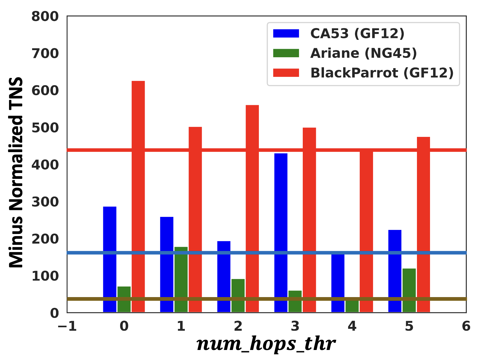
Figure 8: The effect of the threshold $num\_hops\_thr$ applied for timing closure in Equation (1).

VII-C Ablation Study and Autotuning Enhancement

We now discuss the effect of tuning parameters on Hier-RTLMP. There are two common approaches for tuning parameters: (i) ablation study, i.e., sweeping the value of one parameter, the remaining parameters being fixed at their default values; and (ii) autotuning, i.e., applying optimization algorithms like Bayesian optimization [37] to tune multiple parameters simultaneously and figure out the “optimal” parameter combination. In this work, we study both approaches and show the possible PPA (power, performance and area) improvement contributed by parameter tuning. In the following parameter tuning experiments, we use Ariane (NG45) and CA53 (GF12) as our testcases, and tune the parameters $num\_segment$ $(\phi)$ (Section IV-A) and $boundary\_weight$ $(\zeta)$ (Equation (3)). The range of $num\_segment$ $(\phi)$ is [1, 10], and the range of $boundary\_weight$ $(\zeta)$ is [0, 50). Both $num\_segment$ and $boundary\_weight$ are integers, thus there are possible 500 configurations in the search space.

Ablation study. We sweep $num\_segment$ $(\phi)$ values $\{1,2,3,4,5,6,7,8,9,10\}$ and $boundary\_weight$ $(\zeta)$ values $\{0,5,10,15,20,25,30,35,40,45\}$. The best values of $\phi$ and $\zeta$, noted as $\phi^{*}$ and $\zeta^{*}$ respectively, are shown in Table V.

Autotuning. We apply the hyperparameter tuning tool Tune [37] to autotune parameters $\phi$ and $\zeta$. An appropriate loss function is needed to guide the search process [37]. In our use of Tune, we define the loss function as

$$\centering WL\_norm=\frac{1}{|nets|}\sum_{net}{\frac{length(net)}{core.width+core.height}}\@add@centering$$ (4)

$$\centering TNS\_norm=TNS/clock\_period\ \@add@centering$$ (5)

$$\centering Cong=avg\_cong\_hor+avg\_cong\_ver\@add@centering$$ (6)

$$\centering cost=w_{l}\cdot WL\_norm-w_{t}\cdot TNS\_norm+w_{c}\cdot Cong\@add@centering$$ (7)

where wirelength ($WL\_norm$), TNS ($TNS\_norm$) and congestion ($Cong$) are all collected after clock tree synthesis, $core.width$ and $core.height$ are respectively width and height of the fixed outline (Section VI), and $avg\_cong\_hor$ and $avg\_cong\_ver$ are respectively the horizontal and vertical congestion reported by Cadence Innovus 21.1. $w_{l}$, $w_{t}$ and $w_{e}$ are corresponding weights to adjust the values of $WL\_norm$, $TNS\_norm$ and $Cong$ so that they contribute equally to the final cost. Specifically, for Ariane (NG45), $w_{l}$, $w_{t}$ and $w_{e}$ are respectively set to 1.0, 0.1 and 1.0, while for CA53 (GF12), the corresponding values are respectively set to 100, 0.1 and 100. The number of trials allowed to Tune affects QoR: more trials achieve better QoR at the cost of longer tuning time. In our experiments, we set the number of trials to 10 and 50, denoted as $autotune_{10}$ and $autotune_{50}$ respectively. We use 5 threads to obtain an acceptable tuning walltime equal to 2 ($autotune_{10}$) or 10 ($autotune_{50}$) times that of a single Hier-RTLMP run, without any undue CPU needs. The best configurations with respect to loss function found by $autotune_{10}$ and $autotune_{50}$, noted as $autotune_{10}^{*}$ and $autotune_{50}^{*}$ respectively, are shown in Table V. Figure 9 shows the design space explored by $autotune_{50}$. The corresponding best postRouteOpt layouts are presented in Figure 10.

TABLE V: The effects of ablation study and autotuning for Ariane (NG45) and CA53 (GF12). We highlight best values of timing metrics in blue bold font. Data points for GF12 are normalized.

Design (Enablement)	Macro Placer	Std Cell Area ($mm^{2}$)	WL ($m$)	Power ($mW$)	WNS ($ps$)	TNS ($ns$)
Ariane (NG45)	default	0.247	5.27	833	-97	-55
	$\phi^{*}=3$	0.247	5.27	833	-97	-55
	$\zeta^{*}=45$	0.245	5.16	831	-99	-42
	$autotune_{10}^{*}$	0.247	5.28	834	-73	-29
	$autotune_{50}^{*}$	0.247	4.89	837	-76	-30
CA53 (GF12)	default	0.43	1.08	1.03	-0.26	-167
	$\phi^{*}=7$	0.43	1.07	1.03	-0.25	-140
	$\zeta^{*}=15$	0.43	1.08	1.03	-0.26	-167
	$autotune_{10}^{*}$	0.43	1.08	1.03	-0.26	-167
	$autotune_{50}^{*}$	0.43	1.07	1.03	-0.25	-140

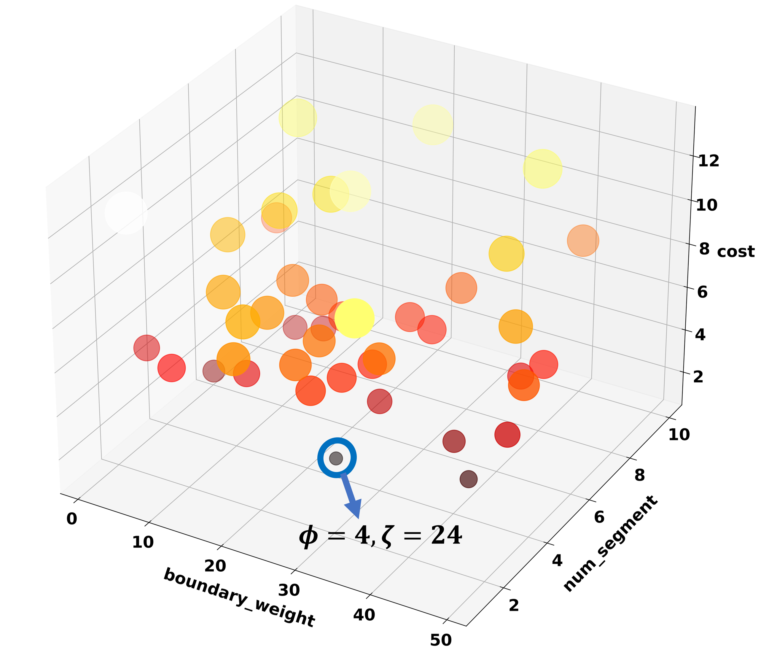
(a)

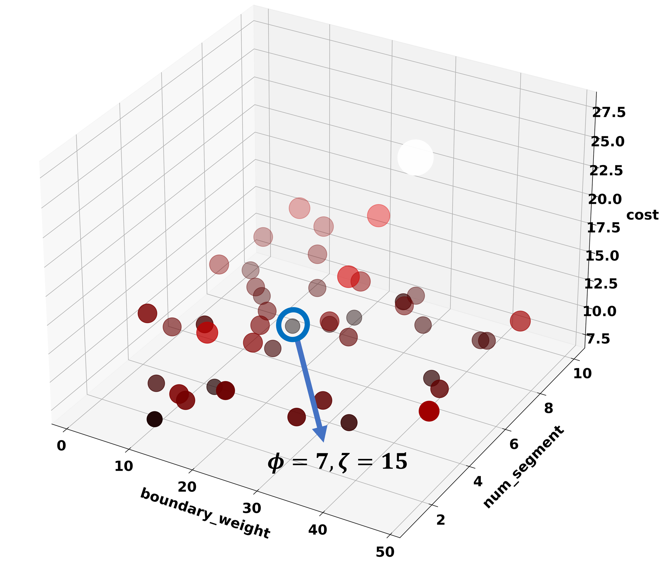
(b)

Figure 9: Design space explored by the $autotune_{50}$. (a) shows the design space explored for Ariane (NG45). The best configuration (num_segment $\phi$ = 4, boundary_weight $\zeta$ = 24) is highlighted in blue circle; and (b) shows the design space explored for CA53 (GF12). The best configuration (num_segment $\phi$ = 7, boundary_weight $\zeta$ = 15) is highlighted in blue circle.

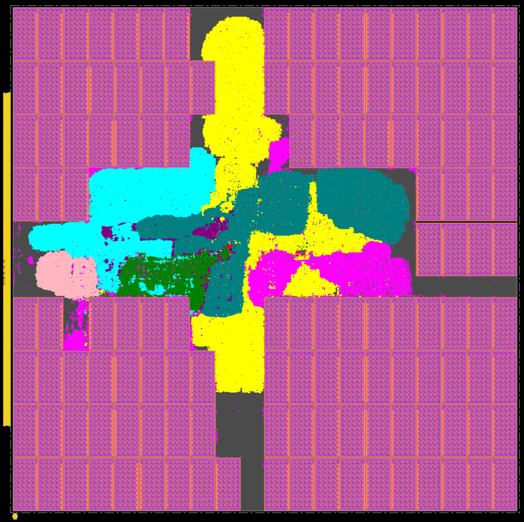
(a)

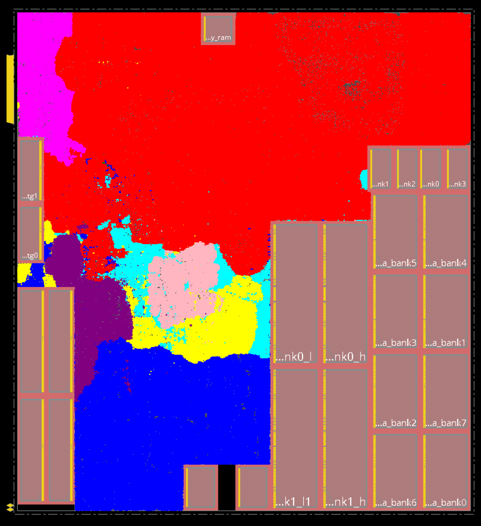
(b)

Figure 10: postRouteOpt layouts corresponding to $autotune_{50}^{*}$, i.e., the best results from autotuning with 50 trials. (a) Ariane (NG45) and (b) CA53 (GF12).

VII-D Runtime Analysis

From Table III, we can see that Hier-RTLMP is much faster than RTL-MP. The profiling result for our macro placer on the Tabla01 (GF12) is shown in Figure 11. We can see that the runtime of sweeping the target dead space $t\_dead\_space$ and target utilization $util$ (Section V) is not significant.

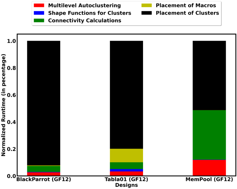
Figure 11: Runtime profiling of Hier-RTLMP on BlackParrot (GF12), Tabla01 (GF12) and MemPool (GF12).

VIII CONCLUSION AND FUTURE WORK

In this work, we propose Hier-RTLMP, which extends RTL-MP to support multilevel physical hierarchy and hierarchical macro placement. Extensions to Hier-RTLMP that we are currently exploring include (i) more intelligent selection of intermediate modules of the logical hierarchy as hierarchical physical clusters based on dataflow and functionality, as well as user tagging of logical modules as hierarchical clusters; (ii) fine tuning of the utilization setting for standard-cell clusters based on the structural complexity, to reduce sweeps and runtime; (iii) autotuning of the cost function based on the level of the physical hierarchy and the contents of clusters, to better preserve dataflow; (iv) enhancing the autoclustering engine to simultaneously identify the appropriate groupings of macros and the clusters of standard cells that “stay together” through the backend flow; and (v) addition of new infrastructure to automatically backtrack up the hierarchy to redo a floorplan placement at a higher-level physical cluster, based on metrics from a lower-level physical cluster.

Acknowledgments. Research at UCSD is partially supported by DARPA IDEA HR0011-18-2-0032 and RTML FA8650-20-2-7009.

Andrew B. Kahng is a distinguished professor in the CSE and ECE Departments of the University of California at San Diego. His interests include IC physical design, the design-manufacturing interface, large-scale combinatorial optimization, AI/ML for EDA and IC design, and technology roadmapping. He received the Ph.D. degree in Computer Science from the University of California at San Diego.

Ravi Varadarajan is currently pursuing the Ph.D. degree at the University of California at San Diego, La Jolla. His research interests include physical design implementation and methodologies.

Zhiang Wang received the M.S. degree in electrical and computer engineering from the University of California at San Diego, La Jolla, in 2022. He is currently pursuing the Ph.D. degree at the University of California at San Diego, La Jolla. His current research interests include partitioning, placement methodology and optimization.

References

- [1] S. N. Adya and I. L. Markov, “Fixed-outline floorplanning: enabling hierarchical design”, IEEE Trans. VLSI 11(6) (2003), pp. 1120-1135.
- [2] R. Bruck, K.-H. Temme and H. Wronn, “FLAIR-a knowledge-based approach to integrated circuit floorplanning”, Proc. Intl. Workshop on Artificial Intelligence for Industrial Applications, 1988, pp. 194-199.
- [3] Y.-C. Chang, Y.-W. Chang, G.-M. Wu, et al., “B*-trees: a new representation for non-slicing floorplans”, Proc. DAC, 2000, pp. 458-463.
- [4] W. Choi and K. Bazargan, “Hierarchical global floorplacement using simulated annealing and network flow area migration”, Proc. DATE, 2003, pp. 1104-1105.
- [5] J. Cong, M. Romesis and J. R. Shinnerl, “Fast floorplanning by look-ahead enabled recursive bipartitioning”, IEEE Trans. CAD 25(9) (2006), pp. 1719-1732.
- [6] T.-C. Chen and Y.-W. Chang, “Modern floorplanning based on -tree and fast simulated annealing”, IEEE Trans. CAD 25(4) (2006), pp. 637-650.
- [7] T. Chen, Y. Chang and S. Lin, “A new multilevel framework for large-scale interconnect-driven floorplanning”, IEEE Trans. CAD 27(2) (2008), pp. 286-294.
- [8] G. Chen, W. Guo, H. Cheng, et al., “VLSI floorplanning based on particle swarm optimization”, Proc. Intl. Conf on Intelligent System and Knowledge Engineering, 2008, pp. 1020-1025.
- [9] C.-C. Hu, D.-S. Chen and Y.-W. Wang, “Fast multilevel floorplanning for large scale modules”, Proc. ISCAS, 2004, pp. 205-208.
- [10] B. H. Gwee and M. H. Lim, “A GA with heuristic-based decoder for IC floorplanning”, Integration 28(2) (1999), pp. 157-172.
- [11] Z. He, Y. Ma, L. Zhang, et al., “Learn to floorplan through acquisition of effective local search heuristics”, Proc. ICCD, 2020, pp. 324-331.
- [12] J. Lu, H. Zhuang, P. Chen, et al., “ePlace-MS: electrostatics-based placement for mixed-size circuits”, IEEE Trans. CAD 24(5) (2015), pp. 685-698.
- [13] M.-C. Kim, N. Viswanathan, C. J. Alpert, et al., “MAPLE: multilevel adaptive placement for mixed-size designs”, Proc. ISPD, 2012, pp. 193–200.
- [14] H. Murata, K. Fujiyoshi, S. Nakatake, et al., “VLSI module placement based on rectangle-packing by the sequence-pair”, IEEE Trans. CAD 15(12) (1996), pp. 1518-1524.
- [15] R. H. J. M. Otten, “Automatic floorplan design”, Proc. DAC, 1982, pp. 261-267.
- [16] K.-H. Temme and R. Bruck, “Chip-architecture planning based on expert knowledge”, Proc. Intl. Workshop on Artificial Intelligence for Industrial Applications, 1998, pp. 188-193.
- [17] J. Z. Yan and C. Chu, “DeFer: Deferred decision making enabled fixed-outline floorplanner”, Proc. DAC, 2008, pp. 161-166.
- [18] Y. Zhan, Y. Feng and S. S. Sapatnekar, “A fixed-die floorplanning algorithm using an analytical approach”, Proc. ASP-DAC, 2006, pp. 771-776.
- [19] A. B. Kahng, J. Lienig, I. L. Markov, et al., VLSI physical design: from graph partitioning to timing closure, Springer, 2nd edition, 2022.
- [20] A. B. Kahng, “Classical floorplanning harmful?”, Proc. ISPD, 2000, pp. 207-213.
- [21] D. H. Kim and S. K. Lim, “Bus-aware microarchitectural floorplanning”, Proc. ASP-DAC, 2008, pp. 204-208.
- [22] M. Ekpanyapong, J. R. Minz, T. Watewai, et al., “Profile-guided microarchitectural floorplanning for deep submicron processor design”, IEEE Trans. CAD 25(7) (2006), pp. 1289-1300.
- [23] A. Mirhoseini, A. Goldie, M. Yazgan, et al., “Chip placement with deep reinforcement learning”, arXiv 2004.10746, 2020.
- [24] A. Mirhoseini, A. Goldie, M. Yazgan, et al., “A graph placement methodology for fast chip design”, Nature 594 (2021), pp. 207-212.
- [25] V. Nookala, Y. Chen, D. J. Lilja, et al., “Microarchitecture-aware floorplanning using a statistical design of experiments approach”, Proc. DAC, 2005, pp. 579-584.
- [26] A. B. Kahng and T. Spyrou, “The OpenROAD project: unleashing hardware innovation”, Proc. GOMACTech, 2021.
- [27] S. Kirkpatrick, C. D. Gelatt and M. P. Vecchi, “Optimization by simulated annealing”, Science 220(4598) (1983), pp. 671-680.
- [28] J. Lin, S. Li and Y. Wang, “Routability-driven mixed-size placement prototyping approach considering design hierarchy and indirect connectivity between macros”, Proc. DAC, 2019, pp. 1-6.
- [29] J.-M. Lin, Y.-L. Deng, Y.-C. Yang, et al., “A novel macro placement approach based on simulated evolution algorithm”, Proc. ICCAD, 2019, pp. 1-7.
- [30] J. Lin, Y. Deng, S. Li, et al., “Regularity-aware routability-driven macro placement methodology for mixed-size circuits with obstacles”, IEEE Trans. VLSI 27(1) (2019), pp. 57-68.
- [31] J.-M. Lin, Y.-L. Deng, Y.-C. Yang, et al., “Dataflow-aware macro placement based on simulated evolution algorithm for mixed-size designs”, IEEE Trans. VLSI 29(5) (2021), pp. 973-984.
- [32] J. K. Ousterhout, “Corner stitching: a data-structuring technique for vlsi layout tools”, IEEE Trans. CAD 3(1) (1984), pp. 87-100.
- [33] X. Tang and D. F. Wong, “FAST-SP: a fast algorithm for block placement based on sequence pair”, Proc. ASP-DAC, 2001, pp. 521-526.
- [34] A. Vidal-Obiols, J. Cortadella, J. Petit, et al., “RTL-aware dataflow-driven macro placement”, Proc. DATE, 2019, pp. 186-191.
- [35] A. Vidal-Obiols, J. Cortadella, J. Petit, et al., “Multi-level dataflow-driven macro placement guided by RTL structure and analytical methods”, IEEE Trans. CAD 40(12) (2020), pp. 2542-2555.
- [36] J. Z. Yan, N. Viswanathan and C. Chu, “An effective floorplan-guided placement algorithm for large-scale mixed-size design”, ACM TODAES 19(3) (2014), pp. 1-25.
- [37] Tune. https://docs.ray.io/en/latest/tune/index.html
- [38] Y. Chuang, G. Nam, C. J. Alpert, et al., “Design-hierarchy aware mixed-size placement for routability optimization”, Proc. ICCAD, 2010, pp. 663-668.
- [39] T.-C. Chen, P.-H. Yuh, Y.-W. Chang, et al., “MP-trees: a packing-based macro placement algorithm for modern mixed-size designs”, IEEE Trans. CAD 27(9) (2008), pp. 1621-1634.
- [40] Y.-C. Liu, T.-C. Chen, Y.-W. Chang, et al., “MDP-trees: multi-domain macro placement for ultra large-scale mixed-size designs”, Proc. ASP-DAC, 2019, pp. 557-562.
- [41] Y. Chen, C. Huang, C. Chiou, et al., “Routability-driven blockage-aware macro placement”, Proc. DAC, 2014, pp. 1-6.
- [42] C.-H. Chiou, C.-H. Chang, S.-T. Chen, et al., “Circular-contour-based obstacle-aware macro placement”, Proc. ASP-DAC, 2016, pp. 172-177.
- [43] C.-H. Chang, Y.-W. Chang and T.-C. Chen, “A novel damped-wave framework for macro placement”, Proc. ICCAD, 2017, pp. 504-511.
- [44] M. Hsu, Y. Chen, C. Huang, et al., “Routability-driven placement for hierarchical mixed-size circuit designs”, Proc. DAC, 2013, pp. 1-6.
- [45] M.-K. Hsu, Y.-F. Chen, C.-C. Huang, et al., “NTUplace4h: A novel routability-driven placement algorithm for hierarchical mixed-size circuit designs”, IEEE Trans. CAD 33(12) (2014), pp. 1914-1927.
- [46] L.-T. Wang, Y.-W. Chang and K.-T. T. Cheng, “Electronic design automation: synthesis, verification, and test”, The Morgan Kaufmann Series in Systems on Silicon, 2009.
- [47] D. F. Wong and C. L. Liu, “A new algorithm for floorplan design”, Proc. DAC, 1986, pp. 101-107.
- [48] Team VLSI, “Floorplan strategies for macro dominating blocks”, 2014. https://www.teamvlsi.com/2021/02/floorplan-strategies-for-macro.html
- [49] The OpenROAD Project. https:github.com/The-OpenROAD-Project/OpenROAD
- [50] TILOS AI Institute, MacroPlacement repository. https://github.com/TILOS-AI-Institute/MacroPlacement
- [51] A. B. Kahng, R. Varadarajan and Z. Wang, “RTL-MP: toward practical, human-quality chip planning and macro placement”, Proc. ISPD, 2022, pp. 3-11.
- [52] H. Esmaeilzadeh, S. Ghodrati, J. Gu, et al., “VeriGOOD-ML: an open-source flow for automated ML hardware synthesis”, Proc. ICCAD, 2021, pp. 1-7.
- [53] Birds-of-a-feather session: open-source EDA and benchmarking summit, Proc. DAC, 2022. https://open-source-eda-birds-of-a-feather.github.io/
- [54] D. Junkin, “Supporting the Scientific method for the next generation of innovators”, DAC-2022 Birds-of-a-Feather presentation. https://open-source-eda-birds-of-a-feather.github.io/doc/slides/BOAF-Junkin-DAC-Presentation.pdf
- [55] Google research “circuit training”. https://github.com/google-research/circuit_training
- [56] BSG black-box SRAM generator repo. https://github.com/jjcherry56/bsg_fakeram
- [57] Ariane RISC-V CPU repo. https://github.com/openhwgroup/cva6
- [58] BlackParrot repo. https://github.com/black-parrot/black-parrot
- [59] MemPool repo. https://github.com/pulp-platform/mempool
- [60] P. Liao, S. Liu, Z. Chen, et al., “DREAMPlace 4.0: Timing-driven global placement with momentum-based net weighting”, Proc. DATE, 2022, pp. 939-944.
- [61] A. Agnesina, P. Rajvanshi, T. Yang, G. Pradipta A. Jiao, et al., “AutoDMP: automated DREAMPlace-based macro placement”, Proc. ISPD, 2023, pp. 149-157.
- [62] Hier-RTLMP, https://github.com/The-OpenROAD-Project/OpenROAD/tree/master/src/mpl2.
- [63] M. Fogaça, A. B. Kahng, E. Monteiro, et al., “On the superiority of modularity-based clustering for determining placement-relevant clusters”, Integration: The VLSI Journal 74 (2020), pp. 32-44.