Computing Controlled Invariant Sets of Nonlinear Control-Affine Systems

Abstract

In this paper, we consider the computation of controlled invariant sets (CIS) of discrete-time nonlinear control-affine systems. We propose an iterative refinement procedure based on polytopic inclusion functions, which is able to approximate the maximal controlled invariant set to within a guaranteed precision. In particular, this procedure allows us to guarantee the invariance of the resulting near-maximal CIS while also computing sets of control inputs which enforce the invariance. Further, we propose an accelerated version of this procedure which refines the CIS by computing backward reachable sets of individual components of set unions, rather than all at once. This reduces the total number of iterations required for convergence, especially when compared with existing methods. Finally, we compare our methods to a sampling based approach and demonstrate the improved accuracy and faster convergence.

I Introduction

Invariance is an important concept for ensuring robustness and safety of control systems. For a dynamical system, a set is (forward) invariant if every trajectory starting in that set remains in the set for all time. For control systems, this notion can be generalized with the determination of a control input which is able to render a set invariant, leading to the notion of a controlled invariant set (CIS). For systems which are subject to uncertainty or noise, the concept of a robust controlled invariant set (RCIS) is critical for safety, as it guarantees invariance in the presence of disturbances.

Controlled invariant sets have been thoroughly studied for linear systems, e.g., [1, 2, 3, 4, 5]. Many of these methods employ iterative procedures based on a one-step backward operator [2, 3] to find backward reachable sets of the system for computing the CIS with high precision. In order to improve the computation time for high-dimensional systems, other non-iterative techniques have also been proposed which rely on lifting to a higher dimensional space to compute the CIS in closed form and projecting the resulting set to the original domain, e.g., [4, 5].

On the other hand, determining controlled invariant sets of nonlinear systems remains a significant challenge. Some works employ convex or zonotopic approximations, e.g., [6, 7], in order to reduce the computational complexity. However, as the maximal controlled invariant sets are nonconvex in general, these methods can be overly conservative.

Another related work pertains to the study of invariant sets of switched systems, e.g., [8, 9, 10], where the input controls switching between a finite number of modes. In that case, the input is easily determined by considering all possible modes and selecting those which lead to invariance [9]. By sampling a continuous set of inputs, these methods can be applied to more general nonlinear systems, but the accuracy and scalability may be limited [10]. These methods result in sets that are guaranteed to be invariant, but the sampling is an additional source of computational complexity as it must be fine enough to properly capture the nonlinear behavior of the system. As a result, these methods are difficult to apply to systems with multiple inputs.

In this paper, we propose two iterative algorithms to compute the near-maximal (non-convex) controlled invariant set of control affine systems up to a guaranteed precision, without sampling the set of allowable inputs. Inspired by [9], our methods use a bisection approach to over- and under-approximate the one-step backward reachable set operator. The main idea of the approach is to compute the forward reachable set of the region of interest, which is described by a union of intervals. The parts of this forward set that are entirely contained in the original set are used as an under-approximation of the backward reachable set. To check the containment, we use polyhedral over-approximations of reachable sets, which allows us to cast the problem of determining the control input as a translation of a polyhedron. This technique allows us to determine a continuous, rather than sampled, set of invariance enforcing control inputs. In addition, we leverage the structure of set unions in the accelerated version, which has the potential to significantly reduce the total number of iterations required for convergence, when compared with existing methods.

I-A Notation

Let $\mathbb{Z}_{\geq 0}$ be the set of nonnegative integers, and ⁿ and ^n×p be the $n$-dimensional Euclidean space, and the set of $n\times p$ matrices, respectively. By means of $\mathcal{B}_{r}$, we denote the $\infty$-norm hyperball of radius $r$. We make use of $\mathbb{I}{}^{n}$ to denote the collection of (multidimensional) intervals of ⁿ, and denote its elements as $[x]\triangleq[\underline{x},\overline{x}]\in\mathbb{I}{}^{n}$ with lower and upper bounds $\underline{x}$ and $\overline{x}$. The function $w([x])$ measures interval width (i.e., $w([x])=\|\overline{x}-\underline{x}\|$ with any vector norm $\|\cdot\|$), $\operatorname{mid}([x])$ selects the midpoint of $[x]$ (i.e., $\operatorname{mid}([x])=\frac{1}{2}(\overline{x}+\underline{x})$), and a function in brackets $[f]([x])$ represents an interval inclusion function (cf. Definition 1). The operator $\oplus$ denotes the Minkowski sum of two sets, and $\ominus$ denotes the Pontryagin difference. For a function $f:{}^{n}\to{}^{m}$ and a set $\mathcal{S}\subset{}^{n}$, $f_{0}(\mathcal{S})$ denotes the image of $\mathcal{S}$ under $f_{0}$. For a bounded polyhedron (polytope) $\mathcal{P}$, we use $H_{\mathcal{P}}$ and $b_{\mathcal{P}}$ to denote the components defining the halfspace representation $\mathcal{P}=\{x\ :\ H_{\mathcal{P}}x\leq b_{\mathcal{P}}\}$. The symbol $V_{\mathcal{P}}$ denotes the vertices of $\mathcal{P}$. Finally, $\operatorname{conv}\mathcal{X}$ denotes the convex hull of the set $\mathcal{X}$.

II Preliminaries

This section introduces preliminary notions that will be used throughout the paper. We begin by defining inclusion functions, which are critical for tractably approximating the images of sets under nonlinear functions.

Definition 1.

Given a function $f:{}^{n}\to{}^{m}$, an inclusion function is an interval function $[f]:\mathbb{I}{}^{n}\to\mathbb{I}{}^{m}$ that satisfies

$$[f]([x])\supseteq f([x]),\ \forall[x]\in\mathbb{I}{}^{n},$$

where $f([x])$ denotes the exact image of $[x]$ under $f$.

The reader is referred to [11, Section 2.4] and [12] for a thorough discussion of different types of inclusion functions, such as natural, centered, etc., as well as mixed-monotone decomposition-based inclusion functions. The results of this paper are not specific to any one type of inclusion function. However, different inclusion functions may produce more or less precise approximations depending on the system.

II-A Translating Polytopes

This section defines two different operations on polytopes: translating one into another, and translating one so it intersects another. These will be used in our algorithm to determine safe control inputs.

Definition 2.

Given two polytopes $\mathcal{P}$ and $\mathcal{Q}$, the set of translations of $\mathcal{P}$ that insert $\mathcal{P}$ into $\mathcal{Q}$ is denoted by

$$\mathcal{I}(\mathcal{P},\mathcal{Q})\triangleq\{r\in{}^{n}:\mathcal{P}\oplus\{r\}\subseteq\mathcal{Q}\}.$$

Similarly, the set of translations of $\mathcal{P}$ that overlap $\mathcal{P}$ with $\mathcal{Q}$ is defined as

$$\mathcal{O}(\mathcal{P},\mathcal{Q})\triangleq\{s\in{}^{n}:\mathcal{P}\oplus\{s\}\cap\mathcal{Q}\neq\emptyset\}.$$

Proposition 1 ([13, Theorem 2.3]).

For polytopes $\mathcal{P}$ and $\mathcal{Q}$,

$$\mathcal{I}(\mathcal{P},\mathcal{Q})=\{r\in{}^{n}:H_{\mathcal{Q}}r\leq b_{\mathcal{Q}}-\beta\},$$

where $\beta_{i}=\max_{v\in V_{\mathcal{P}}}(H_{\mathcal{Q}})_{i}v$. If $\mathcal{P}$ cannot be embedded into $\mathcal{Q}$, then this results in $\mathcal{I}(\mathcal{P},\mathcal{Q})=\emptyset$.

Proposition 2.

Given two polytopes $\mathcal{P}$ with $\mathcal{Q}$,

$$\mathcal{O}(\mathcal{P},\mathcal{Q})=\left\{s\in{}^{n}:\begin{bmatrix}H_{\mathcal{Q}}\\ -H_{\mathcal{P}}\end{bmatrix}s\leq\begin{bmatrix}b_{\mathcal{Q}}-\alpha\\ b_{\mathcal{P}}-\gamma\end{bmatrix}\right\},$$

where $\alpha_{i}=\min_{v\in V_{\mathcal{P}}}(H_{\mathcal{Q}})_{i}v$ and $\gamma_{i}=\min_{v\in V_{\mathcal{Q}}}(H_{\mathcal{P}})_{i}v$.

Proof.

See Appendix -A. ∎

III Invariance Control Problem

Here we introduce the class of systems under consideration and define the concept of controlled invariance. Specifically, we consider nonlinear control affine systems of the form

$$x_{k+1}=f(x_{k},u_{k})\triangleq f_{0}(x_{k})+\sum_{i=1}^{m}g_{i}(x_{k})u_{i,k},$$ (1)

where $x\in{}^{n}$ is the state and $u\in\mathcal{U}\subset{}^{m}$ is the input. We assume that $\mathcal{U}$ is a compact interval, and we will restrict our attention to a region of interest, $\Omega\subset{}^{n}$, which we assume to be given as a finite union of compact intervals.

Assumption 1.

The functions $f_{0}$, and $g_{1}$, $\dots$, $g_{m}$ are Lipschitz continuous, i.e.,

$$\forall i\in\{1,\dots,m\},\ \exists L_{i}\text{ s.t. }\|g_{i}(x)-g_{i}(y)\|\leq L_{i}\|x-y\|,$$

and $$L\text{ s.t. }\|f_{0}(x)-f_{0}(y)\|\leq L\|x-y\|,$$

for every $x,y\in\Omega$.

Next we define the precise notions of invariance which we will consider in this work.

Definition 3.

A set $\mathcal{X}\subset{}^{n}$ is controlled invariant with respect to the dynamics (1) if for every $x_{0}\in\mathcal{X}$, there exists an input $u$ such that $f(x_{0},u)\in\mathcal{X}$.

There are many computational challenges associated with computing controlled invariant sets, many of which arise due to the infinite precision required to adequately handle regions near the boundary of the set. As such, it is convenient to modify the definition to incorporate a robustness margin $r$.

Definition 4.

A set $\mathcal{X}\subset{}^{n}$ is $r$-robustly controlled invariant for system (1) if for every $x_{0}\in\mathcal{X}$, there exists an input $u$ such that $f(x_{0},u)\in\mathcal{X}\ominus\mathcal{B}_{r}$.

Intuitively, in order to be robustly invariant, every point must be mapped into the interior of the set, at some distance $r$ from the boundary.

We are ready to formally state the problem which we aim to address in this paper.

Problem 1 (Controlled Invariant Set Computation).

For a system (1) that satisfies Assumption 1 and a region of interest $\Omega\subset{}^{n}$, given by a union of compact intervals, compute the maximal controlled invariant set contained in $\Omega$ up to a guaranteed precision. Additionally, compute the corresponding set of control inputs that enforces this invariance.

Remark 1.

For ease of exposition, we do not consider any noise or uncertainty in the system dynamics (1). However, it is straightforward to include robustness to bounded noise in our algorithm by increasing the robustness margin $r$.

IV Computation of Controlled Invariant Sets

This section starts by reviewing a well-known iterative procedure for computing maximal controlled invariant sets [14]. After this, we describe our main contribution, which approximates the operator used in each iteration.

Definition 5.

The pre-set, or the one-step backward reachable set of a set $\Omega\subset{}^{n}$ is defined as

$$Q(\Omega)\triangleq\left\{x\in{}^{n}:\exists u\in\mathcal{U}\text{ s.t. }f(x,u)\in\Omega\right\}.$$

We further define the operator

$$I(\Omega)\triangleq Q(\Omega)\cap\Omega,$$

which will enable computation of the maximal controlled invariant set. Repeated application is denoted as $I^{i}(\Omega)=I(I^{i-1}(\Omega))$, $i\in\mathbb{Z}_{\geq 0}$, with $I^{0}(\Omega)=\Omega$. We also define $I_{r}(\Omega)\triangleq Q(\Omega\ominus\mathcal{B}_{r})\cap\Omega$.

Lemma 1 ([14, Special Case of Proposition 4]).

If $\Omega\subset{}^{n}$ is closed, then

$$I^{\infty}\triangleq\lim_{i\to\infty}I^{i}(\Omega)$$

is the maximal controlled invariant set contained in $\Omega$.

This result is the basis for many iterative algorithms, e.g., [2, 3, 14], but there are several computational challenges when dealing with nonlinear systems. In addition to operations involving backward reachability, our algorithm also utilizes operations related to forward reachability, which we define here.

Definition 6.

The one-step forward reachable set of a set $\Omega\subset{}^{n}$ is defined as

$$P(\Omega)\triangleq\{x\in{}^{n}:\exists x_{0}\in\Omega,u\in\mathcal{U}\text{ s.t. }x=f(x_{0},u)\}.$$

The following definition restricts the previous reachable set to that of a particular input, which is used later for determining a suitable controller.

Definition 7.

For a given $u\in\mathcal{U}$, the fixed-control one-step forward reachable set of a set $\Omega\subset{}^{n}$ is defined as

$$P_{u}(\Omega)\triangleq\{x\in{}^{n}:\exists x_{0}\in\Omega\text{ s.t. }x=f(x_{0},u)\}.$$

From the definitions, it is clear that $\bigcup_{u\in\mathcal{U}}P_{u}(\Omega)=P(\Omega)$.

IV-A Polyhedral Approximation of Reachable Sets

Our algorithm will employ polyhedral over-approximations of $P(\Omega)$ and $P_{u}(\Omega)$ to determine feasible control inputs that can lead to invariance.

To this end, we use a decomposition of the function $f$, which we will show to satisfy certain properties. This decomposition will vary depending on the interval $[x]$ under consideration. We first compute $A$ and $\phi$ such that

$$f_{0}(x)=Ax+\phi(x),\ \forall x\in[x],$$ (2)

decomposing $f$ into a linear term plus a remainder. This is always possible (since we can let $A=0$) and can be done in multiple different ways. For example, if $f$ is differentiable, this can be done via linearization about the midpoint of the interval. Another possibility is that $f$ has a bounded Jacobian matrix on $[x]$, in which case we can apply a Jacobian sign-stable decomposition [15, Proposition 2] to compute (2). The method of decomposition will affect the accuracy of the final approximation, as we will discuss at the end of this section. Then, by using an inclusion function $[\Phi]:\mathbb{I}{}^{n}\to\mathbb{I}{}^{n}$ satisfying $[\Phi]([x])\supseteq\phi([x])$, we can guarantee that

$$f_{0}([x])\subseteq A[x]\oplus[\Phi]([x]),$$ (3)

where $A[x]$ denotes the exact (polytope) image of $[x]$ under the linear map $A$.

We also decompose the individual input functions $g_{i}$. For an inclusion function $[g_{i}]$, let $s_{i}=\operatorname{mid}([g_{i}]([x]))$ and $[\Psi_{i}]([x])=[g_{i}]([x])\ominus\{s_{i}\}$, so that

$$g_{i}([x])\subseteq\{s_{i}\}\oplus[\Psi_{i}]([x]),$$ (4)

and $[\Psi_{i}]([x])$ is centered at the origin. A centered $[\Psi_{i}]([x])$ will result in a better approximation later on. We will use the notation $S\in{}^{n\times m}$ and $[\Psi]:\mathbb{I}{}^{n}\to\mathbb{I}{}^{n\times m}$ to denote the matrices with columns $s_{i}$ and $[\Psi_{i}]$, respectively.

In order to guarantee the accuracy of the algorithm, we must first compute bounds on the error of these overapproximations. Assumption 1 allows us to upper bound the width of the resulting inclusion functions.

Proposition 3.

Under Assumption 1, inclusion functions $[\Phi]$ and $[\Psi_{i}]$, $i\in\{1,\dots,m\}$, and constants $\tilde{L}_{i}>0,\ i\in\{0,\dots,m\}$ can be found so that

$$w([\Phi]([x])\leq\tilde{L}_{0}w([x])\ \text{ and }\ w([\Psi_{i}]([x])\leq\tilde{L}_{i}w([x]).$$

for every interval $[x]\subseteq\Omega$.

Proof.

We can, for example, use inclusion functions based on mixed-monotone decompositions (cf. [16, Lemma 1]) or the mean-value form (cf. [11] and [9, Eq. (3)]) that can be shown to satisfy these bounds. ∎

With these decompositions in mind, we can define our approximations of the forward reachable sets. Let

$$\overline{P}([x])\triangleq A[x]\oplus[\Phi]([x])\oplus S\mathcal{U}\oplus[\Psi]([x])\mathcal{U}$$

be the polyhedral overapproximation of the one-step forward reachable set, and let

$$\overline{P}_{u}([x])\triangleq A[x]\oplus[\Phi]([x])\oplus Su\oplus[\Psi]([x])\mathcal{U}$$

be the polyhedral overapproximation of the fixed-control reachable set. The expression $S\mathcal{U}$ denotes the polytopic image of $\mathcal{U}$ under the linear transformation $S$, and $[\Psi]([x])\mathcal{U}$ denotes the interval-valued product of two interval matrices that can be computed using interval arithmetic.

Lemma 2.

Let $\rho\triangleq\tilde{L}_{0}+\max_{1\leq i\leq m}\tilde{L}_{i}w(\mathcal{U}_{i})$. Then for all intervals $[x]\subset\Omega$, the polytopic approximations of the forward reachable sets satisfy

$$P_{u}([x]) \subseteq\overline{P}_{u}([x])\subseteq P_{u}([x])\oplus\mathcal{B}_{\rho w([x])}$$

and

$$P([x]) \subseteq\overline{P}([x])\subseteq P([x])\oplus\mathcal{B}_{\rho w([x])}.$$

Proof.

The inclusion $P_{u}([x])\subseteq\overline{P}_{u}([x])$ is guaranteed by construction, since

$$P_{u}([x])=A[x]\oplus\phi([x])\oplus Su\oplus\sum_{i=1}^{m}\hat{g}_{i}([x]))u_{i},$$

$\phi([x])\subseteq[\Phi]([x])$, and $\hat{g}_{i}([x])\subseteq[\Psi_{i}]([x])$. The inclusion $\overline{P}_{u}([x])\subseteq P_{u}([x])\oplus\mathcal{B}_{\rho w([x])}$ follows from Proposition 3 and the definition of the Minkowski sum. The second statement is proved in the same way. ∎

IV-B Interval Approximation of Pre-Sets

We describe our main contribution next, which is a novel algorithm for approximating the operator $I$ for systems of the form (1). Given a union of compact intervals $\Omega$, we propose an iterative refinement procedure that approximates $I(\Omega)$ by another union of compact intervals. Algorithm 1 summarizes the main steps of this process, described in detail next.

Algorithm 1 $\underline{I}(\Omega)$

1:$\Omega$, $\varepsilon$

2:$Q\leftarrow\{\Omega\}$, $N\leftarrow\emptyset$, $\underline{I}\leftarrow\emptyset$, $\mathcal{E}\leftarrow\emptyset$, $\mathcal{U}_{I}\leftarrow\emptyset$

3:while $Q\neq\emptyset$ do

4:     $[x]\leftarrow\operatorname{pop\_front}(Q)$

5:     Compute $A$, $\Phi$, $s_{i}$, and $\Psi_{i}$ on $[x]$

6:     if $\overline{P}([x])\cap\Omega=\emptyset$ then

7:         $N\leftarrow N\cup[x]$

8:     else if $\exists u\in\mathcal{U}\text{ s.t. }\overline{P}_{u}([x])\subseteq\Omega$ then

9:         $\underline{I}\leftarrow\underline{I}\cup[x]$

10:         $\mathcal{U}_{I}\leftarrow\mathcal{U}_{I}\cup([x],S^{\dagger}(S\mathcal{U}([x])))$

11:     else if $w([x])\leq\varepsilon$ then

12:         $\mathcal{E}\leftarrow\mathcal{E}\cup[x]$

13:     else

14:         $(l,r)\leftarrow\operatorname{bisect}([x])$

15:         $\operatorname{push\_front}(Q,l)$

16:         $\operatorname{push\_front}(Q,r)$

17:     end if

18:end while

19:return $\underline{I}$, $\mathcal{U}_{I}$

The algorithm is a loop that operates on a queue ($Q$) of intervals. An element of the queue is retrieved (and removed) from the front of the queue using the $\operatorname{pop\_front}$ operation, while an element is added to the front of the queue using the $\operatorname{push\_front}$ operation. The following steps are implemented until the queue is empty. Every interval $[x]$ is checked to see whether it may be part of the pre-set of $\Omega$. Two tests are performed:

1. Is the forward reachable set from $[x]$ disjoint with $\Omega$? If so, $[x]$ is disjoint from $I(\Omega)$.

2. Can an input $u$ be found so that the reachable set from $[x]$, restricted to the input $u$, lies entirely within $\Omega$? If so, $[x]\subset I(\Omega)$.

If either condition is satisfied, then the set $[x]$ is saved in lists labeled $\mathcal{N}$ (the collection of intervals disjoint with $I(\Omega)$) and $\mathcal{S}$ (the collection of intervals contained in $I(\Omega)$).

If neither condition is satisfied and the $[x]$ is wider than the specified tolerance, it is bisected along its largest dimension and both resulting intervals are added to the front of the queue using the $\operatorname{push\_front}$ operation. Otherwise, $[x]$ is added to $\mathcal{E}$, which is a collection of the so-called “indeterminate” sets, which are neither disjoint from nor subsets of $I(\Omega)$.

Line 8 of Algorithm 1 requires checking the condition

$$\exists u\in\mathcal{U}\text{ s.t. }\overline{P}_{u}([x])\subseteq\Omega,$$ (5)

which is a nonconvex feasibility problem, due to the nonconvexity of $\Omega$. Luckily, we can exploit the structure of both $\overline{P}_{u}([x])$ and $\Omega$ in order to efficiently and precisely compute the set of $u$ that satisfy (5).

Notice that, in the definition of $\overline{P}_{u}$, the term $A[x]\oplus[\Phi]([x])\oplus[\Psi]([x])\mathcal{U}$ is a convex polyhedron, and the additive term $Su$ serves only to translate the resulting polyhedron. On the other hand, $\Omega$ is a union of intervals, and also more generally a union of polyhedra. Therefore, we can reduce the feasibility problem in (5) to a problem of translating a polyhedron into a union of polyhedra. We describe here an equivalence which helps solve this problem, inspired by [17].

Lemma 3.

Let $\mathcal{P}=\operatorname{conv}(\Omega\cap\overline{P}([x]))$ and $\mathcal{Q}=\mathcal{P}\setminus(\Omega\cap\overline{P}([x]))$. Then, the following statements are equivalent:

1. $\exists u\in\mathcal{U}\text{ s.t. }\overline{P}_{u}([x])\subseteq\Omega$;

2. $S\mathcal{U}([x])\triangleq\mathcal{I}(\overline{P}_{0}([x]),\mathcal{P})\setminus\mathcal{O}(\overline{P}_{0}([x]),\mathcal{Q})\neq\emptyset.$

Proof.

By defining $\overline{P}_{0}([x])\triangleq A[x]\oplus[\Phi]([x])\oplus[\Psi]([x])\mathcal{U}$, we obtain that for any $u$, $\overline{P}_{u}([x])=\overline{P}_{0}([x])\oplus\{Su\}$. Furthermore, $\overline{P}([x])=\overline{P}_{0}([x])\oplus S\mathcal{U}$. This gives rise to the equivalance

$$\exists u\in\mathcal{U}\text{ s.t. }\overline{P}_{u}([x])\subseteq\Omega$$

$$\iff\exists r\in{}^{n}\text{ s.t. }\overline{P}_{0}([x])\oplus\{r\}\subseteq\Omega\cap\overline{P}([x]),$$

where it must be true that $r=Su$. We see that by intersecting with $\overline{P}([x])$ on the right hand side, we can identify a translation by a vector $r$, which is automatically restricted to the range of $S$. To find the $r$ in the latter expression, we first find the translations into the convex hull of $\Omega\cap\overline{P}([x])$ (i.e., $\mathcal{I}(\overline{P}_{0}([x]),\mathcal{P})$), then remove the translations that cause overlap with parts of the convex hull that are not in the original set (i.e., $\mathcal{O}(\overline{P}_{0}([x]),\mathcal{Q})$). This gives the set of translations $r$ that result in containment in $\Omega\cap\overline{P}([x])$, therefore yielding the expression for $S\mathcal{U}([x])$. ∎

Since $S\mathcal{U}([x])$ is the difference between a polytope and a union of polytopes, it can be expressed as the union of a finite number of polytopes. The equivalence in Lemma 3 gives us a tractable method of solving the feasibility problem in (5), using procedures to efficiently compute $\mathcal{I}$ and $\mathcal{O}$. Finally, since $\forall r\in S\mathcal{U}([x]),\ \exists u\in\mathcal{U}$ such that $r=Su$, we can recover the set of inputs with the Moore-Penrose pseudoinverse, $\mathcal{U}([x])=S^{\dagger}(S\mathcal{U}([x]))$, which is stored/saved in $\mathcal{U}_{I}$ as pairs $([x],\mathcal{U}([x]))$.

Remark 2.

The computation of the set difference between two polyhedra can be represented as a union of polyhedra. This procedure is computationally expensive, especially when considering the difference between a polyhedron and a union of polyhedra, for which the best algorithms [18] have exponential complexity. In fact, the computation of set differences is the largest computaional burden of our method. Caching of results from previous iterations may reduce the number of differences that must be computed in the final implementation, although these details are not described here for the sake of brevity. $\bullet$

We finish this section by proving that Algorithm 1 returns a useful approximation of $I(\Omega)$, which is within some known bound of the maximal CIS.

Lemma 4.

Let $\Omega$ be a finite union of compact intervals. Then, for any precision $\varepsilon>0$, Algorithm 1 terminates in a finite number of iterations. Furthermore, letting $\underline{I}(\Omega)$ denote the output of Algorithm 1, it holds that

$$I(\Omega\ominus\mathcal{B}_{\rho\varepsilon})\subseteq I_{\rho\varepsilon}(\Omega)\subseteq\underline{I}(\Omega)\subseteq I(\Omega).$$ (6)

Proof.

The proof is similar to [9, Lemma 1], relying on the bounds provided by Lemma 2. ∎

IV-C Near-Maximal Controlled Invariant Sets

With the ability to compute $\underline{I}(\Omega)$ using Algorithm 1, all that remains is to repeat this operation until convergence is achieved. Algorithm 2 describes this simple procedure, which is guaranteed to terminate in finite time.

Algorithm 2 Approximation of $I^{\infty}(\Omega)$

1:$\Omega$, $\varepsilon$

2:$I_{0}\leftarrow\Omega$, $I_{1}\leftarrow\emptyset$

3:while $I_{0}\neq I_{1}$ do

4:     $I_{1}\leftarrow I_{0}$

5:     $I_{0}\leftarrow\underline{I}(I_{0})$ $\triangleright$ via Algorithm 1

6:end while

7:return $I_{0}$

Theorem 1.

For any finite union of compact intervals $\Omega$ and precision $\varepsilon>0$, Algorithm 2 terminates in a finite number of iterations. Furthermore, denoting the output of the algorithm as $\underline{I}^{\infty}(\Omega)$, the following inclusions hold:

$$I_{r}^{\infty}(\Omega)\subseteq\underline{I}^{\infty}(\Omega)\subseteq I^{\infty}(\Omega),$$

where $r=\rho\varepsilon$. Finally, $\underline{I}^{\infty}(\Omega)$ is controlled invariant.

Note that it is possible for the algorithm to return an empty set only if the system does not admit an $r$-robustly controlled invariant set, meaning $I_{r}^{\infty}=\emptyset$.

Proof.

Let $\underline{I}^{k}(\Omega)$ denote the value of $\underline{I}(\underline{I}^{k-1}(\Omega))$ in the $k$-th iteration, with $\underline{I}^{0}(\Omega)=\Omega$. Since the algorithm terminates if $\underline{I}^{k-1}(\Omega)=\underline{I}^{k}(\Omega)$, we only need to consider the case when they are not equal. In this case, the structure of Algorithm 1 is such that $\underline{I}^{k}(\Omega)\subsetneq\underline{I}^{k-1}(\Omega)$. Since $\Omega$ is compact, $\underline{I}^{k}(\Omega)$ contains only a finite number of intervals which will be considered using the bisection method for a given $\varepsilon$. Then $\exists K\geq 0$ such that $\underline{I}^{k}(\Omega)=\emptyset,\ \forall k\geq K$, meaning the algorithm terminates in finite time.

To prove the inclusions, note that by Lemma 4, $I_{r}(\Omega)\subseteq\underline{I}(\Omega)\subseteq I(\Omega)$. Also, for any two sets $A\subseteq B\subseteq{}^{n}$, we know that $\underline{I}(A)\subseteq\underline{I}(B)$ and $I_{r}(A)\subseteq I_{r}(B)$. Therefore by applying Lemma 4 and induction, we can determine that $I_{r}^{k}(\Omega)\subseteq\underline{I}^{k}(\Omega)\subseteq I^{k}(\Omega)$ for all $k\geq 0$.

Finally, to prove invariance of $\underline{I}^{\infty}(\Omega)$, note that by Lemma 4, $\underline{I}^{\infty}(\Omega)=\underline{I}(\underline{I}^{\infty}(\Omega))\subseteq I(\underline{I}^{\infty}(\Omega))$. ∎

Remark 3 (An Outside-In Approach).

The method described in this paper is commonly known as an outside-in method, since we start with a region of interest $\Omega$ and search for the largest invariant set $\mathcal{X}=I^{\infty}(\Omega)$ which it contains. It is also possible to use an inside-out approach, which starts with a known invariant set, and iteratively grows that set [10]. Our method can be easily adapted for this case, as well. $\bullet$

To conclude this section, we state a result that has the potential to significantly reduce the number of iterations required by Algorithm 2, hence, accelerating convergence. Let $\{\Omega_{i}\}_{i=1}^{N}$ be any ordered collection of sets such that $\Omega=\bigcup_{i=1}^{N}\Omega_{i}$. Define the operator

$$I_{i}(\Omega)\triangleq\bigcup_{j\neq i}\Omega_{j}\cup\left(Q(\Omega)\cap\Omega_{i}\right),$$

and let $I_{1:N}\triangleq I^{N}(\cdots(I^{1}(\Omega))$. We let the $I_{i}$ operator preserve the order of the constituent subsets by defining

$$(I_{i}(\Omega))_{i}=Q(\Omega)\cap\Omega_{i}\quad\text{and}\quad(I_{i}(\Omega))_{j}=\Omega_{j},\ j\neq i.$$

Theorem 2.

For a closed set $\Omega\subseteq{}^{n}$, $I_{1:N}$ satisfies

$$I_{1:N}(\Omega)\subseteq I(\Omega),\text{ and }$$

$$\lim_{k\to\infty}(I_{1:N})^{k}(\Omega)=\lim_{k\to\infty}I^{k}(\Omega)=I^{\infty}(\Omega).$$ (7)

Proof.

By definition, for any $i\neq j$,

$$I_{i}(I_{j}(\Omega)) =\bigcup_{\ell\neq i}I_{j}(\Omega)_{\ell}\cup\left(Q(I_{j}(\Omega))\cap I_{j}(\Omega)_{i}\right)$$

$$=\bigcup_{\ell\neq i,\ell\neq j}\Omega_{\ell}\,\cup\left(Q(\Omega)\cap\Omega_{j}\right)\cup\left(Q(I_{j}(\Omega))\cap I_{j}(\Omega)_{i}\right)$$

$$\subseteq\bigcup_{\ell\neq i,\ell\neq j}\Omega_{\ell}\cup\left(Q(\Omega)\cap(\Omega_{i}\cup\Omega_{j})\right),$$

since $I_{j}(\Omega)_{i}\subseteq\Omega_{i}$ and $Q(I_{j}(\Omega))\cap I_{j}(\Omega)_{i}\subseteq Q(\Omega)\cap\Omega_{i}$. By applying this statement recursively, we arrive at

$$I_{1:N}(\Omega)\subseteq\bigcup_{i=1}^{N}\Omega_{i}\cap Q(\Omega)=I(\Omega).$$ (8)

In (7), since $I_{1:N}$ is monotonically decreasing and closed, the limit exists. We will show by induction that for all $k\geq 0$, $(I_{1:N})^{k}(\Omega)\supseteq I^{\infty}(\Omega)$. Consider a point $x\in I^{\infty}(\Omega)$. We know $x\in Q(I^{\infty}(\Omega))\subseteq Q(\Omega)$. Therefore, by the definition of $I_{1}$, $x\in I_{1}(\Omega)$, meaning $I_{1}(\Omega)\supseteq I^{\infty}(\Omega)$. By repeating this reasoning for $I_{2},\dots,I_{N}$, we can see that $I_{1:N}(\Omega)\supseteq I^{\infty}(\Omega)$. For the step case, assume that $(I_{1:N})^{k-1}(\Omega)\supseteq I^{\infty}(\Omega)$. Then by the same argument as the base case, for any $x\in I^{\infty}(\Omega)$, $x\in Q(I^{\infty}(\Omega))\subseteq Q((I_{1:N})^{k-1}(\Omega))$, implying $(I_{1:N})^{k}(\Omega)\supseteq I^{\infty}(\Omega)$. Using this fact in combination with (8), monotonicity of $I$ and $I_{1:N}$, and an induction argument proves (7). ∎

Theorem 2 is useful because it allows us to independently consider individual regions of the invariant set, rather than approximating the $I$ operator all at once. Essentially, our procedure can focus on $I_{i}(\Omega)$ without needing to compute all of $Q(\Omega)$, which is more expensive. Using the $I_{i}$ operator often leads to a reduction in the total number of iterations required. Algorithm 3 describes the modified procedure that takes advantage of this fact. In the algorithm, $\Omega$ is updated whenever an interval is determined to not be a part of the invariant set. The loop terminates if every interval in the queue has been checked since $\Omega$ was last changed, meaning every interval is contained in the invariant set. The function $\operatorname{checked}$ tracks whether a given $[x]$ has been tested against the current $\Omega$. It defaults to $0$, and is assigned a value of $1$ after $[x]$ is processed. Note that $\operatorname{push\_back}$ places an item in the back of the queue.

Algorithm 3 Accelerated Approximation of $I^{\infty}(\Omega)$

1:$\Omega$, $\varepsilon$

2:$Q\leftarrow\{\Omega\}$, $N\leftarrow\emptyset$, $\underline{I}\leftarrow\emptyset$, $\mathcal{E}\leftarrow\emptyset$, $\mathcal{U}_{I}\leftarrow\emptyset$

3:while $\exists[x]\in Q$, $\operatorname{checked}([x],\Omega)=0$ do

4:     $[x]\leftarrow\operatorname{pop\_front}(Q)$

5:     Compute $A$, $\Phi$, $s_{i}$, and $\Psi_{i}$ on $[x]$

6:     if $\overline{P}([x])\cap\Omega=\emptyset$ then

7:         $N\leftarrow N\cup[x]$

8:         $\Omega\leftarrow\Omega\setminus[x]$

9:     else if $\exists u\in\mathcal{U}\text{ s.t. }\overline{P}_{u}([x])\subseteq\Omega$ then

10:         $\operatorname{checked}([x],\Omega)\leftarrow 1$

11:         $\operatorname{push\_back}(Q,[x])$

12:         $\mathcal{U}_{I}\leftarrow\mathcal{U}_{I}\cup([x],S^{\dagger}(S\mathcal{U}([x])))$

13:     else if $w([x])\leq\varepsilon$ then

14:         $\mathcal{E}\leftarrow\mathcal{E}\cup[x]$

15:         $\Omega\leftarrow\Omega\setminus[x]$

16:     else

17:         $(l,r)\leftarrow\operatorname{bisect}([x])$

18:         $\operatorname{push\_front}(Q,l)$

19:         $\operatorname{push\_front}(Q,r)$

20:     end if

21:end while

22:$\underline{I}^{\infty}\leftarrow\bigcup_{[x]\in Q}[x]$

23:return $\underline{I}^{\infty}$, $\mathcal{U}_{I}$

Lemma 5.

For any finite union of compact intervals $\Omega$ and precision $\varepsilon>0$, Algorithm 3 returns the same result as Algorithm 2. Furthermore, the number of iterations required by Algorithm 3 is less than or equal to the number required by Algorithm 2.

Proof.

The first statement can be proved by the same reasoning as Theorem 1. The second statement arises from the inclusion $I_{1:N}(\Omega)\subseteq I(\Omega)$ (cf. Theorem 2) and can also be seen by direct comparison of the algorithms. ∎

V Examples and Comparisons

In this section, we demonstrate the effectiveness of our approach on a numerical example, i.e., an inverted pendulum on a cart. We also compare our approach to the method for switched systems in [9], where the input space is sampled/gridded and considered as controlled modes.

As in [9], we consider an inverted pendulum on a cart, discretized using forward Euler with a sampling time of $0.01\text{s}$. The dynamics are

$$\dot{x}_{1} =x_{2},$$

$$\dot{x}_{2} =\frac{mgl}{J}\sin(x_{1})-\frac{b}{J}x_{2}+\frac{l}{J}\cos(x_{1})u,$$

with parameters $m=0.2$ kg, $g=9.8$ $\text{m}/\text{s}^{2}$ , $l=0.3$ m, $J=0.006$ $\text{kg}\cdot\text{m}^{2}$, and $b=0.1$ $\text{N}/\text{m}/\text{s}$. This system and its discretization are control affine. We consider a region of interest $\Omega=[-0.05,-0.05]\times[-0.01,0.01]$ and an input set $\mathcal{U}=[-0.1,0.1]$.

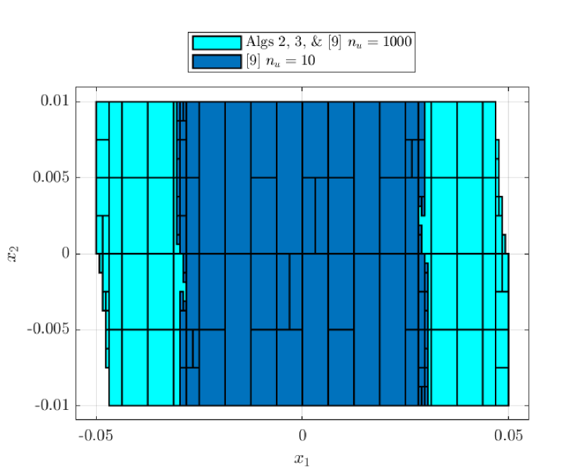
Figure 1: Controlled invariant sets of the inverted pendulum system.

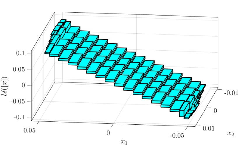
Figure 2: Union of invariance-enforcing inputs $\mathcal{U}([x])$ identified by Lemma 3.

Figure 1 shows the identified controlled invariant sets for our approaches, i.e., using Algorithms 2 and 3, and that of [9], with $n_{u}=10$ and $n_{u}=1000$ sampled inputs. All methods were run with a precision $\varepsilon=0.001$. On the other hand, Figure 2 shows the union of all invariance-enforcing control inputs $\mathcal{U}([x])$ identified by Algorithms 2 and 3. Finally, Table I shows a comparison of computation times with different parameters.

Method	$\varepsilon$	Iterations	Time (s)	Volume
Algorithm 2	$10^{-3}$	703	0.54	97.9%
Algorithm 3	$10^{-3}$	618	0.63	97.9%
[9] ($n_{u}=10$)	$10^{-3}$	10729	0.12	59.8%
[9] ($n_{u}=1000$)	$10^{-3}$	485	0.59	97.9%

TABLE I: Computational comparison between Algorithm 2, Algorithm 3, and [9]. $n_{u}$ denotes the number of input samples taken uniformly across $\mathcal{U}$. The volume is given in % of the original $\Omega$.

Evidently, our method is able to identify a larger CIS in fewer iterations than the sampling and interval arithmetic based approach in [9], when the number of samples is small. This is presumably due to the higher accuracy of our polytopic approximations, and the fact that we consider the entire continuous range of control inputs. Increasing the number of sampled inputs results in a better approximation of the CIS, at the cost of some additional computation time.

VI Conclusion

We proposed two methods for approximating controlled invariant sets of nonlinear control-affine systems using an iterative refinement approach. We used techniques from computational geometry involving translations of polyhedra to allow us to efficiently compute continuous sets of feasible control inputs, rather than using a sampling approach with switched dynamics. We demonstrated the effectiveness of our method on a numerical example, which showed improved accuracy over existing methods and led to faster convergence in some cases. In the future, we will further explore the extension of our approach to continuous time, as well as the control synthesis problem, including some notions of optimality, while also investigating ways to improve the accuracy and efficiency of our algorithms. We also will test our approaches on a wide variety of nonlinear systems.

-A Proof of Proposition 2

We begin by stating two intermediate results which will be used to prove the proposition. The first allows us to determine whether two polytopes intersect by examining the hyperplanes defining each polytope.

Proposition 4.

Given two polytopes $\mathcal{P}$ and $\mathcal{Q}$, $\mathcal{P}\cap\mathcal{Q}\neq\emptyset$ if and only if both of the following statements are true

1. $\mathcal{P}$ intersects every halfspace defining $\mathcal{Q}$, i.e., $\forall i\in\{1,\dots,N_{\mathcal{Q}}\},\ \exists p_{i}\in\mathcal{P}$ such that $(H_{\mathcal{Q}})_{i}p_{i}\leq(b_{\mathcal{Q}})_{i}$.

2. $\mathcal{Q}$ intersects every halfspace defining $\mathcal{P}$, i.e., $\forall i\in\{1,\dots,N_{\mathcal{P}}\},\ \exists q_{i}\in\mathcal{Q}$ such that $(H_{\mathcal{P}})_{i}q_{i}\leq(b_{\mathcal{P}})_{i}$.

Proof.

Necessity is simple, since if $\mathcal{P}\cap\mathcal{Q}\neq\emptyset$, every $v\in{\mathcal{P}\cap\mathcal{Q}}$ will satisfy the existence conditions in 1) and 2).

To prove sufficiency, note that $\mathcal{P}\cap\mathcal{Q}=\emptyset$ if and only if there exists a separating hyperplane, defined by some $h_{*}\in{}^{n}$ and $b_{*}\in\real$, such that $\forall v\in\mathcal{P},\ h^{\top}v\leq b$ and $\forall v\in\mathcal{Q},\ h^{\top}v>b$. Conditions 1) and 2) preclude the existence of this separating hyperplane, implying $\mathcal{P}\cap\mathcal{Q}\neq\emptyset$. ∎

The second intermediate result tells us how to translate a polytope so that it intersects a given halfspace.

Proposition 5.

Given a polytope $\mathcal{P}$ and halfspace $\mathcal{H}=\{x:h^{\top}x\leq b\}$, the set of translations, i.e., of $\mathcal{P}$ that intersect $\mathcal{H}$; i.e. $\mathcal{O}(\mathcal{P},\mathcal{H})\triangleq\{s\in{}^{n}:\mathcal{P}\oplus\{s\}\cap\mathcal{H}\neq\emptyset\}$, is given by

$$\mathcal{O}(\mathcal{P},\mathcal{H})=\{s\in{}^{n}:\ h^{\top}s\leq b-\alpha\},$$

where $\alpha=\min_{v\in V_{\mathcal{P}}}h^{\top}v$.

Proof.

The reasoning is similar to [13, Theorem 2.3], with $\min$ replacing $\max$ because intersection, rather than containment, is required. ∎

Proposition 2 follows from the combination of Proposition 4 with repeated application of Proposition 5 to every halfspace defining both $\mathcal{P}$ and $\mathcal{Q}$ (with $-s$ replacing $s$ in the second part, as the translation is applied to $\mathcal{P}$, not $\mathcal{Q}$).

References

- [1] F. Blanchini, “Set invariance in control,” Automatica, vol. 35, no. 11, pp. 1747–1767, 1999.
- [2] M. Fiacchini and M. Alamir, “Computing control invariant sets in high dimension is easy,” arXiv preprint, 2018.
- [3] M. Rungger and P. Tabuada, “Computing robust controlled invariant sets of linear systems,” IEEE Transactions on Automatic Control, vol. 62, no. 7, pp. 3665–3670, 2017.
- [4] T. Anevlavis and P. Tabuada, “Computing controlled invariant sets in two moves,” in 2019 IEEE 58th Conference on Decision and Control (CDC), 2019, pp. 6248–6254.
- [5] T. Anevlavis, Z. Liu, N. Ozay, and P. Tabuada, “An enhanced hierarchy for (robust) controlled invariance,” in 2021 American Control Conference (ACC), 2021, pp. 4860–4865.
- [6] M. Fiacchini, T. Alamo, and E. Camacho, “On the computation of convex robust control invariant sets for nonlinear systems,” Automatica, vol. 46, no. 8, pp. 1334–1338, 2010.
- [7] L. Schäfer, F. Gruber, and M. Althoff, “Scalable computation of robust control invariant sets of nonlinear systems,” submitted to IEEE Transactions on Automatic Control. Available from https://mediatum.ub.tum.de/doc/1663416/document.pdf, 2022.
- [8] S. Jang, N. Ozay, and J. L. Mathieu, “An invariant set construction method, applied to safe coordination of thermostatic loads,” arXiv preprint, 2022.
- [9] Y. Li and J. Liu, “Invariance control synthesis for switched nonlinear systems: An interval analysis approach,” IEEE Transactions on Automatic Control, vol. 63, no. 7, pp. 2206–2211, 2018.
- [10] J. Bravo, D. Limon, T. Alamo, and E. Camacho, “On the computation of invariant sets for constrained nonlinear systems: An interval arithmetic approach,” Automatica, vol. 41, no. 9, pp. 1583–1589, 2005.
- [11] L. Jaulin, M. Kieffer, O. Didrit, and E. Walter, “Applied interval analysis,” ed: Springer, London, 2001.
- [12] M. Khajenejad and S. Z. Yong, “Tight remainder-form decomposition functions with applications to constrained reachability and guaranteed state estimation,” IEEE Transactions on Automatic Control, pp. 1–16, 2023.
- [13] I. Kolmanovsky and E. Gilbert, “Theory and computation of disturbance invariant sets for discrete-time linear systems,” Mathematical Problems in Engineering, vol. 4, pp. 317–367, 01 1998.
- [14] D. Bertsekas, “Infinite time reachability of state-space regions by using feedback control,” IEEE Transactions on Automatic Control, vol. 17, no. 5, pp. 604–613, 1972.
- [15] M. Khajenejad, F. Shoaib, and S. Z. Yong, “Interval observer synthesis for locally Lipschitz nonlinear dynamical systems via mixed-monotone decompositions,” in American Control Conference (ACC), 2022, pp. 2970–2975.
- [16] M. Khajenejad and S. Z. Yong, “Simultaneous input and state interval observers for nonlinear systems with full-rank direct feedthrough,” in IEEE Conference on Decision and Control, 2020, pp. 5443–5448.
- [17] B. Baker, S. Fortune, and S. Mahaney, “Polygon containment under translation,” Journal of Algorithms, vol. 7, no. 4, pp. 532–548, 1986.
- [18] M. Baotic, “Polytopic computations in constrained optimal control,” Automatika, vol. 50, pp. 119–134, 04 2009.