Silent Abandonment

Silent Abandonment in Contact Centers: Estimating Customer Patience from Uncertain Data Antonio Castellanos, Galit B. Yom-Tov, Yair Goldberg antonio.cas@campus.technion.ac.il, gality@technion.ac.il, yairgo@technion.ac.il Technion—Israel Institute of Technology

In the quest to improve services, companies offer customers the opportunity to interact with agents through contact centers, where the communication is mainly text-based. This has become one of the favorite channels of communication with companies in recent years. However, contact centers face operational challenges, since the measurement of common proxies for customer experience, such as knowledge of whether customers have abandoned the queue and their willingness to wait for service (patience), are subject to information uncertainty. We focus this research on the impact of a main source of such uncertainty: silent abandonment by customers. These customers leave the system while waiting for a reply to their inquiry, but give no indication of doing so, such as closing the mobile app of the interaction. As a result, the system is unaware that they have left and waste agent time and capacity until this fact is realized. In this paper, we show that 30%–67% of the abandoning customers abandon the system silently, and that such customer behavior reduces system efficiency by 5%–15%. To do so, we develop methodologies to identify silent-abandonment customers in two types of contact centers: chat and messaging systems. We first use text analysis and an SVM model to estimate the actual abandonment level. We then use a parametric estimator and develop an expectation-maximization algorithm to estimate customer patience accurately, as customer patience is an important parameter for fitting queueing models to the data. We show how accounting for silent abandonment in a queueing model improves dramatically the estimation accuracy of key measures of performance. Finally, we suggest strategies to operationally cope with the phenomenon of silent abandonment.

Missing Data, Service Operations, Abandonment, Customer Patience, Information Uncertainty, Expectation Maximization, Survival Analysis

1 Introduction

The field of service engineering relies on the ability to measure proxies for customer experience in a service system. Two of the most common operational measures that are used as such proxies are customer waiting and abandonment of the queue. Both are crucial measures of performance for understanding customer’s willingness to wait for service, which in turn is crucial for making operational decisions (Mandelbaum and Zeltyn 2013, Garnett et al. 2002). Waiting happens when a customer enters the service system, but the system does not have an available service agent to serve her. Abandonment (Ab) naturally occurs when such waiting is too long and exceeds the customer’s willingness to wait (henceforth, patience). Different streams of literature study different aspects of customer patience, such as its distribution (e.g., Gans et al. 2003), its connection to service utility (e.g., Aksin et al. 2013), its manipulation (e.g., Armony et al. 2009, Aksin et al. 2017), and more. But, the literature on the estimation of customer patience and its implications for the optimization of operational decisions (e.g., staffing and routing) assumes accurate and complete knowledge of customer abandonment. However, when studying some contact centers, we face the problem of not being able to know whether a customer abandoned or received service, as we will explain shortly. This uncertainty creates a situation where the company is unsure of the service quality they provide to their customers and how efficiently they use their resources. This in turn may lead to problematic operational decisions.

In this paper, we concentrate on a specific type of uncertainty that relates to a specific type of customer behavior in contact centers. We term the behavior in question silent abandonment (Sab). A Sab customer is a customer that leaves the system while waiting in the queue but gives no indication of doing so in real time (i.e., she does not close the chat window/application when abandoning). Therefore, when an agent becomes available, the (abandoning) customer is assigned to that agent. Only after all of the agent’s inquiries go unanswered for some time does the agent (or system) realize that the customer has abandoned the queue without notifying the system and the agent (or system) closes the chat. We find that this situation creates two problems of information uncertainty: (a) missing data: the system may not be aware (even in retrospect) whether a customer silently abandoned the queue or was served. Most companies assume the latter, thereby biasing quality measurements (for a detailed definition of the concept of missing data see Little and Rubin 2002); and (b) censored data: the system may be aware that the customer silently abandoned the queue but it does not know exactly when, thereby censoring the data on customer patience (for a discussion of censored data see Smith 2002). In addition, Sab customers create two operational problems of agent efficiency: (a) idleness: the agent waits for inquiries from a customer that is no longer there; and (b) wasted work: the agent tries to solve problems that have already been solved by the customer herself or by another agent (such as when the customer writes an inquiry before entering the queue and then abandons the queue and uses a different channel of communication such as a phone call), thereby, creating confusion, frustration, and wasted effort. We note that silent abandonment is more likely to happen when the system is overloaded with customers and waits are long. During such periods a significant number of the agents are likely to be either idle or “busy” with abandoning customers, wasting critically needed capacity. Moreover, during these times, the Sab customers are taking the places of customers that want service and are actually waiting in the queue. Finally, we note that silent abandonment results in inaccurate measurements of queue length. Therefore, any algorithm that uses that information (e.g., for delay announcement; see Armony et al. 2009, Ibrahim and Whitt 2009) would need to be adjusted to allow for silent abandonment.

The context of this research is contact centers, which are an important part of the digital revolution the service industry is undergoing. Services are becoming ever more automatic and easy to use, as service companies branch into more accessible service channels such as mobile applications. Technology allows modern-day companies to replace traditional service encounters (face-to-face, telephone) with technology-mediated service encounters (Massad et al. 2006, van Dolen and de Ruyter 2002), which allow customers and service employees to be in different locations and connect via a technological interface (Schumann et al. 2012, Froehle and Roth 2004). Nowadays employees and customers can interact through social media (e.g., Twitter or Facebook), corporate websites (e.g., chats), or messaging applications (e.g., WhatsApp and WeChat). This enables customers to interact with agents through contact-center platforms similar to those that they use to contact their family and friends. Therefore, it should come as no surprise that contact centers are slowly substituting call centers as the preferred way for customers to communicate with companies. Indeed, a survey conducted by a cloud-based communications provider found that 78% of the customers preferred to text with the company rather than call their call center (RingCentral 2012).

Our paper uses data from two types of contact centers: chat and messaging service systems. In chat services the customers communicate with the company via a web browser while in messaging services the communication is typically through a mobile application. Even though they are very similar in the sense that customers communicate with agents via short text messages, there are important differences between the two that relate to the main challenges of this paper regarding information uncertainty. In Section 2 we describe in detail how the operations of these two systems differ and present the data we have from each one.

It is worthy noting that the digital revolution provides the service industry with new opportunities to improve services (Rafaeli et al. 2017, Altman et al. 2019) but also with new operational challenges. Operating chat- and messaging-based contact centers is substantially different from operating call centers. For example, in chat and messaging service systems, unlike in call centers or face-to-face services, agents can provide service to multiple customers concurrently (Goes et al. 2018, Tezcan and Zhang 2014, Luo and Zhang 2013). We claim that the information uncertainty that results from the phenomenon of silent abandonment creates a need to redefine the basic methods of measuring quality and efficiency, as well as to develop methodologies to estimate customer patience. This is the focus of this paper. We also show that models that account for the silent-abandonment phenomenon and incorporate the methodologies we develop here fit the data of chat and messaging centers much more accurately than a regular Erlang-A model (Palm 1957). Finally, we measure and discuss the implications of silent abandonment on system performance and managerial practices.

The phenomenon of silent abandonment may appear also in healthcare systems. For example, in emergency departments (ED) a patient may abandon the queue but tell no one, leaving without being seen (LWBS) by a medical practitioner. ED abandonment increases the risk of a patient suffering an adverse outcome, increases the probability of the patient returning (in the study of Baker et al. 1991, 51% of the abandoning patients saw a physician within a week of leaving the system), and impacts hospital revenue (Batt and Terwiesch 2015). According to Medicare (2018), the national average of LWBS patients was 2% during 2018, for US EDs.

Closely related to the phenomenon of silent abandonment in contact centers is the phenomenon of patients’ no-shows to medical appointments. A no-show customer does not arrive to a scheduled appointment and fails to notify the system in advance. This creates censored data similar to silent abandonment, but not missing data, since in hindsight complete information is observed regarding patient service (or lack thereof). The scope of no-show customers can be as high as 23% to 34% (Liu 2016). Ho and Lau (1992) showed that no-shows strongly affect system performance because of loss of capacity and forced idleness of physicians. This is something that we claim happens also in contact centers. Several methodologies have been suggested to cope with no-show customers, such as overbooking (Vissers 1979) and reminders (Geraghty et al. 2008). However, in contact centers arrivals are not known in advance, and therefore other mechanisms are needed to cope with the phenomenon. Another difference between no-show customers and Sab customers relates to our points (a) and (b) regarding agent efficiency, presented above. In medical appointments it can be observed whether a patient shows or does not show up for her appointment, and this information is realized as soon as her service is supposed to start (without delay). Therefore, in the no-show case the agent can immediately start serving the next patient instead of waiting for the one who does not show up (assuming that there is a next patient at the clinic). But in contact centers, since the customer is not physically present in front of the agent, there is no indication that the customer has abandoned the queue and this information is realized only after a few minutes of wasted agent effort. Therefore, overbooking can mitigate the efficiency loss of no-shows, whereas silent abandonment requires other solutions, as we suggest in Section 5.

Another closely related phenomenon is service failure. For example, Carmeli et al. (2019) analyzed the impact of service failure (they called it abandonment during service) on the design of Interactive Voice Response (IVR) systems and websites, where a customer may or may not successfully complete a self-service. They show the impact of estimating the proportion of customers that had an unsuccessful service (17%) on system design. In the present paper, we only consider queue abandonment, and make a similar claim that silent abandonment has an impact on system design.

Our research can also be related to research on queue inference, where queue statistics are deduced from limited information; e.g., Larson (1990). However, to the best of our knowledge no work has addressed the problem of missing data in our context.

1.1 Research Goals

The present paper concentrates on the following goals:

Estimate the scope of the silent-abandonment phenomenon. We want to estimate how many customers silently abandon the queue in contact centers. This is similar to estimating the scope of queue abandonment in healthcare. In fact, our goal is to be more precise than prior studies, by analyzing silent abandonment at the level of the individual customer. Hence, we attempt to solve the missing data problem. In Section 3 we construct classification models that estimate the probability of silent abandonment by a specific customer. Using data on customer and agent behavior, we analyze, among other things, customer sojourn time as well as the text messages of the customer and agent. We find that around one-third of the abandoning customers in the chat system dataset, and around two-thirds in the messaging system dataset, are Sab customers.

Create an algorithm to estimate customer patience in the presence of silent abandonment. Gans et al. (2003) reviewed methods for estimating customer patience, based on call-center applications. As we mentioned, customer behavior in contact centers differs from customer behavior in call centers. To our knowledge no paper has attempted to estimate customer patience in contact centers, although finite patience has been considered in optimization models of contact centers (cf. general patience in Long et al. 2018 and exponential patience in Tezcan and Zhang 2014). To estimate call-center patience, Mandelbaum and Zeltyn (2013) assumed that customer patience time, $T$, and virtual wait time, $W$, are exponentially distributed with rates $\theta$ and $\gamma$, respectively. Specifically, they developed a maximum likelihood estimator for estimating customer patience from right-censored data. Inspired by the LWBS phenomenon in EDs, Yefenof et al. (2018) extended their estimator to left-censored patience data, which is created by patients who do not announce their abandonment time. (To that end, they developed both parametric and non-parametric methods.) As we will demonstrate later, their estimators are suitable for estimating customer patience in chat systems, where the only type of information uncertainty that exists is censored data. However, in messaging systems, system design and silent abandonment create both of the above-mentioned types of uncertainty in the data (i.e., censored data and missing data). Therefore, we develop a new method for estimating customer patience that addresses the additional problem of missing data. In Section 4, we develop an expectation-maximization algorithm to estimate customer patience given both types of information uncertainty. It is important to estimate system parameters as accurately as possible, since performance measures of queueing systems are sensitive to inaccuracies in such estimations (Whitt 2006). We show in Section 5 that, indeed, a more accurate estimation of customer patience, one that takes into account the phenomenon of silent abandonment, significantly improves the fit of the queueing model to the data.

Analyze the operational implications of silent abandonment. In Section 5, we develop a queueing model that captures the dynamics of contact centers in the presence of silent abandonment. We estimate the amount of time companies waste due to the phenomenon of silent abandonment, and analyze the implications of such wasted time on system performance. We conclude with a discussion of how a bot or a classification model for identifying silent abandonment in real time may be used to reduce the impact of Sab customers on the system.

2 Data and Research Setting

For the purposes of our research we have acquired and analyzed data from both of the aforementioned contact centers, namely, chat and messaging systems. The data was provided by LivePerson Inc., a company that builds computational infrastructures for the contact-center industry. As mentioned above, the differences in the way chat and messaging contact centers operate and in the way people use them have an impact on information uncertainty. Therefore, both environments will be used for this research. The description of the two systems and their data is given in the following two subsections.

2.1 Chat Systems

Chat systems are used for browser-based, one-time, short interactions (around 12 minutes on average) with service companies. The process of communication is as follows: a customer requests service by pressing a “contact us” button on the company website. Once the request for service arrives to the system, the system assigns the customer to a service agent. If no service agent is available, the customer enters a queue and waits for an assignment to an available agent. An agent can serve multiple customers concurrently: the maximal level of concurrency in the chat data is three customers per agent. The agent sends a greeting to indicate to the customer that she can proceed to write her inquiry. The full interaction contains several agent and customer messages that the two parties send one another. Due to concurrency, agent response time may also include short waits (if the agent is busy answering another customer).

The data is extracted from 18,497 service interactions conducted in February 2017. The data includes general information on each chat as well as on each line written. Each chat is identified by chat ID, employee ID, date, the amount of time the customer waited in the queue before the chat started, whether the customer abandoned the queue by closing the chat window and at what time, the time an agent was assigned to that chat, the time the chat ended, the device used for the communication, type of service (e.g., sales or support), and more. Each chat line in the data contains the following information: a time-stamp of when the line was sent, a notation of who wrote that line (customer, agent, or system), and the number of words written in the line. The data also includes information on the work status of each service agent (online, offline, on break, or idle) during the workday. Each agent’s load is estimated by analyzing the agent’s activities with customers when the agent is online.

The contact center is open 7 days a week from 8:00 to 22:00. The average number of arrivals per hour is 51.58 customers. The arrival rate varies with the hours of the day. The pattern of the hourly arrival rate is typical of service systems. The mean number of agents working per hour is 12.45. Within our data, the average customer length of stay (LOS), or chat duration, is 11.65 minutes ($SD=9.98$) (the average includes the LOS of the Sab customers). The average wait time in queue is 2.37 minutes ($SD=3.88$).

2.2 Messaging Systems

Messaging systems are typically used for interacting with known customers, i.e., as part of a long-term relationship the company has with that customer. The communication is usually conducted through smart-phone applications, such as Facebook, WeChat, or iMessage. Compared to chats, we observe that messaging interactions generally have a much longer duration: around 49.2 minutes. The interaction is more casual than in chat systems, and the messaging service reinforces this notion to customers by sending them an automatic message instructing them to address the service as if “talking to a friend.” A very important difference between messaging and chat systems is that in messaging systems a customer initiates a service request by writing a detailed inquiry. As a result, explicit information regarding the customer’s problem is known before she enters the queue. This small difference is the first source of information uncertainty we mentioned in the Introduction: missing data. Because operational data does not indicate whether a service was provided or not, we need to analyze the written text in order to gain such an indication. We will elaborate on this fact in more detail in Section 3.

We acquired, from a messaging contact center, data on 337,224 service interactions conducted during the month of May 2017. It includes detailed information on all the conversations (exactly as with the chat data). The messaging system operates 24/7, and it has a higher load than the chat system. The average number of arrivals is 594.79 per hour. The arrival rate varies with the hours of the day in accord with a typical service system pattern. The mean number of online agents per hour is 134.69. The mean concurrency level of agents is around 5.4 customers per agent ($SD=4$). Average customer LOS (from entering the queue until the last message was written in that conversation) is 49.2 minutes ($SD=64$), including LOS of Sab customers. The average wait in the queue is 9.28 minutes ($SD=20.4$).

3 Estimating the Scope of Silent Abandonment as a Source of Information Uncertainty

In this section we aim to build models to define which conversations can be classified as silent abandonment with high probability. This will enable us to estimate the percentage of Sab customers. In addition, such information also enables us to estimate the time it takes for the service agents to realize that a Sab customer has abandoned the queue. We conduct separate analyses of the two types of contact centers we are working with (chat systems and messaging systems) due to the difference in their service process.

3.1 Estimating the Scope of Silent Abandonment in Chat Systems

The company that provided us with the chat system dataset erroneously estimates the percentage of abandoning customers by counting only customers that left the system by closing the window of the interaction. Indeed, those customers provided a clear indicator that they abandoned the system. We refer to this type of customer abandonment as known abandonment (Kab). The proportion of Kab customers in the chat data is 14%. We claim that this is an underestimation of the proportion of abandoning customers since it ignores the phenomenon of silent abandonment. That is, the chat company does not account for the customers that arrived to the system, got assigned to an agent, but did not communicate with that agent at all—but instead clearly abandoned the system during wait time. Since these customers gave no indication that they were leaving, the system was unaware of their abandonment and assigned them to an agent. Therefore, we can identify the conversations in which customers silently abandoned the queue by indicating whether the conversations include system and agent messages but do not include any customer messages. Using this method, we found that Sab customers constitute 6% of all customers arriving to the chat system. Therefore, the correct estimation of the probability of abandonment is 20%, emphasizing our claim that the company is unaware of the actual service level it provides. Moreover, out of all the abandoning customers, 30% abandon the queue silently.

We can use the silent-abandonment classification to estimate the time it takes for an agent to realize that the customer actually (silently) abandoned the queue. It takes, on average, 4.32 minutes ($SD=7.15$) for it to happen. This is the time in which the agent keeps trying to communicate with the customer and gets no reply, i.e., the time the agent “wastes” on that customer. Therefore, if we subtract the silent-abandonment conversations from the conversation data we see that the average served customer LOS is 12.25 minutes ($SD=10.683$). Of those 12.25 minutes, 51% are customer response time and 49% are agent response time. From the agent’s perspective, 7% of the chats she handles during the day are silent-abandonment chats and 93% are served customer chats. We can compute the percentage of time agents spent on silent-abandonment chats by dividing the time spent on Sab conversations by total work time. Hence,

$$\text{Effort}=\frac{0.07*4.32}{0.07*4.32+0.93*12.25*0.49}=0.05,$$

i.e., agents spent 5% of their work time engaging in Sab conversations. We will show the impact of this effort in Section 5.

3.2 Estimating the Scope of Silent Abandonment in Messaging Systems

In the case of the messaging system, the company also underestimates the proportion of abandoning customers by taking into account only the known abandonments. The proportion of Kab customers in the messaging dataset is 7.2% of the customer population, much lower than in the chat dataset. Here the classification of silent abandonment is much more problematic due to the problem of missing data. As mentioned, in messaging systems, the customers usually write down their problems before entering the queue and, therefore, it is hard to distinguish between short conversations in which the customer was shortly served—those with at least one agent reply to the customer inquiry but no customer reaction—and conversations in which the customer silently abandoned the queue before the agent replied—those with agent requests for further details from the customer but no customer reaction. In other words, a customer who is shortly served is a customer who writes an inquiry, the agent solves the problem (as is clear from the agent’s reply), but the customer is impolite and does not even say “Thank you.” By contrast, the Sab customer writes an inquiry, the agent replies but does not solve the problem (e.g., the agent asks for additional information), and the customer does not respond any further. With this description in mind, we can see that to know which customer silently abandons the queue, in messaging systems, we need to take a closer look at the conversation text.

We refer to the whole group of uncertain conversations in messaging systems, which includes both the short-service and the silent-abandonment conversations, as uncertain silent abandonment (uSab) conversations. In the messaging dataset, this group accounts for 26.2% of all the conversations. Figure 1 presents two examples of uncertain silent abandonment conversations. Figure 1(a) gives an example of a short-service conversation where the customer inquiry was solved, while Figure 1(b) gives an example of a silent-abandonment conversation where the customer abandoned the queue without indication.

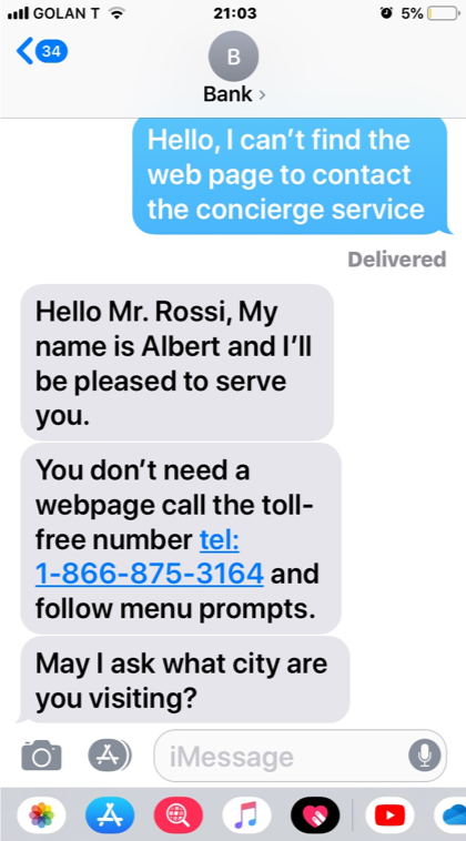
(a) Short-service Conversation

(b) Silent-abandonment Conversation

Figure 1: Examples of Uncertain Silent-Abandonment Messaging Conversations

Next, we build an automated classification model to distinguish the conversations of customers who silently abandoned the queue. The dataset we use comprises a random sample of 550 uSab conversations. We manually tag those conversations into the two groups—short-service or silent abandonment—by reading the text of the whole service interaction. We compare the performance of several machine-learning classification methods: logistic regression (stepwise backward and with a ridge penalty), support-vector machines (SVM), k-nearest neighbors (k-NN), and classification tree (additionally, we pruned the tree). The classification models use textual features extracted from the conversation transcript as well as meta-data, such as wait time and system load, as described in Section 2.2. The data is randomly separated into training and test sets containing 75% and 25% of the conversations, respectively. We denote by $\pi_{i}$ the probability that customer $i$ silently abandoned the queue, given that this conversation is part of the uncertain silent abandonment group. Formally, $\pi_{i}\triangleq Pr\left\{silent\;abandonment_{i}\mid uncertain\;silent\;abandonment_{i}\right\}$. Using the above methods, we are able to estimate $\pi_{i}$, for each individual conversation $i$.

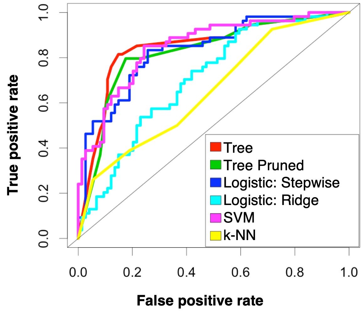
Figure 2: ROC Curve

Table 1: Area under the ROC

Model	AUC
SVM	0.85
Tree	0.85
Logistic Regression: Stepwise	0.83
Tree Pruned	0.82
Logistic Regression: Ridge	0.71
k-NN	0.65

We compare the classification models using the Receiver Operating Characteristic (ROC) curve, presented in Figure 2. The ROC plots the True Positive Rate (TPR) against the False Positive Rate (FPR) for varying threshold levels. The ROC curve is a recognized method for comparing performance of different classification methods in a visualized way and for selecting the best threshold to work with (Fawcett 2006). A standard characteristic in that regard is the area under the ROC curve (AUC), presented in Table 1. Using this criterion, we conclude that the best classification methods for our problem are the SVM model and the classification tree, for which the AUC is 0.85. Models with an AUC above 0.80 are considered “excellent” classification models (Hosmer and Lemeshow 2002). Details about SVM and the classification tree can be found in Appendix 7. The SVM model includes, among other things, the following features: specific words written in the conversation, customer experience (e.g., amount of time the customer waited in the queue), and agent’s work time (e.g., amount of time the agent engaged with the customer). To select a specific threshold level for the SVM model, we find the threshold that maximizes the sensitivity (TPR) and specificity (1-FPR) proportions, i.e., maximizes the proportion of silent-abandonment and short-service conversations that are correctly identified. We find that the optimal threshold is 0.47 with a sensitivity proportion (TPR) of 85% and a specificity proportion (1-FPR) of 76%.

With this information, we are able to obtain $\hat{\pi_{i}}$ for every uSab conversation in our full messaging dataset and to state that out of the group of uSab conversations, which constituted 26.2% of all the conversations in the messaging data, 55% are silent-abandonment conversations and 45% are short-service conversations. This means that the actual proportion of abandoning customers in this dataset is 21.6%, far above the estimation of 7.2% abandonment that the company currently has. Moreover, out of all the abandoning customers, we find that 67% are Sab customers (14.4% of all arriving customers). This information highlights the importance of taking Sab customers into account in order to correctly evaluate performance levels in contact centers.

To estimate the LOS of a customer that (silently) abandoned the queue and could not be served, we calculate the average conversation duration of the silent-abandonment conversations (using the above 0.47 threshold). We find that it takes, on average, 19.37 minutes ($SD=26.68$) for an agent to identify a silent-abandonment conversation. This is the average time that channel capacity is wasted while the agent tries to communicate with the departed customer (note that she might be serving other customers concurrently). Given the uncertain conversation classification, we can estimate that the average duration of short-service conversations is 55.63 minutes ($SD=105.77$). This finding reveals that shortly served customers have a longer LOS than Sab customers, which is not easily observed in the distribution of the LOS.

Measuring agent effort in treating Sab customers, we find that 15.5% of the inquiries that the agent answers are from Sab customers, 12.7% from short-service customers and 71.8% are from served customers. Dividing the time spent on Sab conversations by the total work time reveals that agents spent 11% of their work time dealing with Sab conversations:

$$\text{Effort}=\frac{0.155*19.37}{0.155*19.37+0.127*55.63+0.718*49.2*0.4891}=0.11.$$ (1)

The effort wasted on Sab customers in the messaging system is two times higher than in the chat system, showing how a small change in the service process in contact centers can drive system inefficiency. This finding highlights the importance of identifying silent abandonment as soon as possible, to improve system efficiency.

4 Estimating Customer Patience with Silent Abandonment

Our next problem is to estimate customer patience in contact centers. As mentioned in Section 1.1, data on customer patience is censored. When the customer abandons the queue and provides an indication of doing so—a known abandonment—she provides exact information regarding her patience. Indeed, her patience equals her wait time. However, how long the customer would be required to wait if she were to stay in the queue, i.e., her virtual wait time, is unknown. Therefore, patience acts as a lower bound for virtual wait time. When the customer is served, her wait time is actually a lower bound for her true patience. Therefore, the data is right-censored by the virtual wait time (itself uncensored). This type of right-censoring was studied by Mandelbaum and Zeltyn (2013) using call-center data; we refer to their estimator as Method 1. In contrast to call centers, in contact centers data on patience is also left-censored due to the silent-abandonment phenomenon. Indeed, when a customer abandons the queue without indicating that she has done so—a silent abandonment—her wait time equals her virtual wait time (itself uncensored); thus, the wait time is an upper bound for her real patience as her patience was clearly less than her wait time. Yefenof et al. (2018) addressed this situation, motivated by LWBS in EDs; we refer to their estimator as Method 2. As we mentioned, in chat systems we have complete data; therefore, Method 2 can be used to estimate customer patience since similar conditions exist. We apply Method 2 to chat data in Section 5. But messaging systems require a new methodology for patience estimation, because of the added complexity missing data brings to customer classification. Indeed, this situation requires a different approach, which will be the focus of this section. In Section 4.1 we develop our expectation-maximization (EM) algorithm for estimating customer patience in messaging systems, and in Section 4.2 we validate its accuracy, sensitivity, and robustness.

4.1 The EM Algorithm: Model Assumption and Formulation

The problem of missing information on uSab customers stems from the fact that we do not know whether they received short service, in which case their patience would be right-censored, or whether they silently abandoned, in which case their patience would be left-censored. Nonetheless, we know that the length of time these customers waited in the queue, and hence their virtual wait time is uncensored.

Following the formulation of Yefenof et al. (2018), let $T$ be customer patience time (failure time) and assume that it has a cumulative distribution function (cdf) $F$ and a probability distribution function (pdf) $f$. Assume that $T\sim exp(\theta)$. This assumption follows Brown et al. (2005) who showed, using call-center data on served and abandoning customers, that patience distribution has an exponential tail. We also show, in Section 5, that queueing models with exponentially distributed patience fit contact-center data better compared to queueing models with generally distributed patience, providing further support for our assumption. Let $W$ be the virtual wait time (censoring time), i.e., the time the customer is required to wait by the system, and assume that it has a cdf $G$ and a pdf $g$. We know from queueing theory that in overloaded systems, like the contact centers we are investigating, wait time is close to exponentially distributed (Kingman 1962). In addition, Brown et al. (2005) showed that in call-center data with served and abandoning customers, virtual wait time is close to exponentially distributed. In our dataset we have served and abandoning customers; hence, we can make a realistic assumption that the virtual wait time is exponentially distributed. This assumption is confirmed by fitting an exponential distribution to the simulated virtual wait time distribution in the queueing model in Section 5. Formally, assume that $W\sim exp(\gamma)$. Let $\Delta$ be an indicator for the case where the customer lost patience before the agent replied, i.e., $\Delta\triangleq 1_{\{T\leq W\}}$. Conversations in which information regarding $\Delta_{i}$ is missing are assigned a null value. Let $Y$ be a random variable indicating whether the customer will inform the system when abandoning. We assume that $Y\sim Bernoulli(q)$, where $q$ is the probability that the customer will inform the system when abandoning; formally, $q\triangleq Pr\left\{Indicate\;abandonment\right\}$.

Assume that $W$ and $T$ are independent, as is frequently done in right-censoring survival analysis (e.g., Smith 2002, Mandelbaum and Zeltyn 2013, Yefenof et al. 2018). Moreover, this is a natural assumption in contact centers since patience is decided by the individual customer while the virtual wait time is decided by the company. This is indeed the case in our contact centers where no delay information is provided to the customer, such as her place in queue (that may remind her that she is waiting in the queue). Additionally, we assume that $Y$ and $W$ are independent. That is, the decision of a customer to indicate whether she is abandoning the queue is independent of her wait time. For example, a customer might tend to leave windows open in the computer even if she is not using them; therefore, this tendency would be independent of the wait time. We assume that $Y$ and $W$ are independent for tractability reasons; currently we don’t have evidence to support this assumption and suggest that it be relaxed in future research. Finally, let $U$ be the system’s observed time. For each arriving customer $i$ we observe the vector of data $(U_{i},Y_{i},\Delta_{i})$, $i=1,...,n$.

Summarizing, our model rests on the following assumption:

1. Patience time is $T\sim exp(\theta)$.

2. Virtual wait time is $W\sim exp(\gamma)$.

3. Customer abandonment indicator is $Y\sim Bernoulli(q)$.

4. $W$ and $T$ are independent.

5. $Y$ and $W$ are independent.

4.1.1 Customer Classes with Complete Data.

In Table 2 we formally define three customer classes under the assumption of complete data on which customers abandoned. The table identifies each customer class by type, notation indicator, and formal definition (based on values $\Delta$ and $Y$, and observed time $U$).

Table 2: Classes of Customers: Complete Data

Class Type	Notation Indicator	Formal Definition	$\Delta$	$Y$	$U$
Service	$C_{1}=1$	$1-\Delta$	0	0	$W$
Known Abandonment	$C_{2}=1$	$Y\Delta$	1	1	$T$
Silent Abandonment	$C_{3}=1$	$(1-Y)\Delta$	1	0	$W$

Remark: Note that in chat systems the data on which customers abandoned is complete; i.e., there are no missing values in $\Delta$. Therefore, we can categorize the conversations into the above three classes with complete certainty; i.e., we know exactly to which class each customer belongs.

4.1.2 Customer Classes with Missing Data.

Due to the problem of missing data on the uSab conversations in the messaging system, we are not able to categorize all the conversations into just one of the classes we defined in Section 4.1.1. Therefore, we need to formulate additional class indicators. Let $M$ denote the customer classes in a system in which there is missing data on which individual customers abandoned. These classes are defined in Table 3.

Table 3: Classes of Customers: Missing Data

Class Type	Notation	Formal Definition	$\Delta$	$Y$	$U$
Service	$M=1$	$1-\Delta$	0	0	$W$
Known Abandonment	$M=2$	$Y\Delta$	1	1	$T$
Uncertain Silent Abandonment	$M=0$	$1-\Delta$ or $(1-Y)\Delta$	null	0	$W$

Formally:

$$M^{i}=1 \Longrightarrow C_{1}^{i}=1.$$

$$M^{i}=2 \Longleftrightarrow C_{2}^{i}=1.$$

$$M^{i}=0 \Longrightarrow C_{1}^{i}=1\text{ or }C_{3}^{i}=1.$$

4.1.3 The EM Algorithm Formulation.

The EM algorithm estimates the following parameters simultaneously: the rate at which customers lose patience, $\theta$, the probability of informing the system when abandoning, $q$, and the rate of the virtual wait time distribution, $\gamma$. The optimization problem is defined to maximize the likelihood function. The likelihood function measures the probability that the observations are given from the assumed distributions given the parameters ($\theta,q,\gamma$). We write the likelihood of the observed data $D\triangleq\{(U_{i},Y_{i},\Delta_{i}),$ $i=1,...,n\}$ as follows:

$$L(D;\theta,q,\gamma)= \prod_{i=1}^{n}\left\{e^{-\theta U_{i}}\gamma e^{-\gamma U_{i}}\right\}^{C_{1}^{i}}\left\{q\theta e^{-\theta U_{i}}e^{-\gamma U_{i}}\right\}^{C_{2}^{i}}\left\{(1-q)(1-e^{-\theta U_{i}})\gamma e^{-\gamma U_{i}}\right\}^{C_{3}^{i}}$$ (2)

$$= \prod_{i=1}^{n}\left\{e^{-\theta U_{i}}\gamma e^{-\gamma U_{i}}\right\}^{1-\Delta_{i}}\left\{q\theta e^{-\theta U_{i}}e^{-\gamma U_{i}}\right\}^{\Delta_{i}Y_{i}}\left\{(1-q)(1-e^{-\theta U_{i}})\gamma e^{-\gamma U_{i}}\right\}^{(1-Y_{i})\Delta_{i}.}$$

The function is formulated following Yefenof et al. (2018): the first part is for the the served customer ($C_{1}^{i}=1$), where we multiply the survival function of the customer patience ($1-F_{T}\left(u\right)$) by the pdf of the customer’s wait time. The second part is for the known-abandonment customer ($C_{2}^{i}=1$), where we multiply the probability of informing when abandoning by the pdf of the customer patience and the survival function of the customer’s wait time ($1-G_{W}\left(u\right)$). Finally, the third part is for the Sab customer ($C_{3}^{i}=1$), where we multiply the probability of not informing when abandoning by the cdf of the customer patience and the pdf of the customer’s wait time.

However, this likelihood function depends on knowing the complete data. Recall that some of the observations belong to the class $M=0$ since they have missing data in $\Delta$. Therefore, we cannot find the parameters by simply solving the maximization problem. Instead, we need to formulate an EM algorithm (see Algorithm 1), a well-known computing strategy for dealing with problems of missing data including censoring, since censoring is a special case of missing data (see Chapters 7 and 8 of Little and Rubin 2002). The algorithm estimates the parameters ($\theta,q$, $\gamma$), using Theorems 4.1 and 4.2. Specifically, it estimates starting parameter values and subsequently iterates between the expectation step (E-step)—using Theorem 4.1—and the maximization step (M-step)—using Theorem 4.2—and updates these estimators until convergence. In the $t$th iteration, the E-step consists of finding a surrogate function (given in Equation (3)) that is a lower bound on the log-likelihood function (given in Equation (7)) and is tangent to the log-likelihood at $(\widehat{\theta^{(t)}},\widehat{q^{(t)}},\widehat{\gamma^{(t)}})$. In practice, it is enough to compute the expectation of the log-likelihood given the information of the previous iteration, which is presented in Equation (LABEL:eq:ci) of Theorem 4.1.

$$l(D,\theta,q,\gamma) =\sum_{i=1}^{n}\left\{\left(\widehat{C_{1,t}^{i}}\right)\left(\log\gamma-\gamma U_{i}-\theta U_{i}\right)\right\}$$ (3)

$$+\sum_{i=1}^{n}\left\{\left(\widehat{C_{2,t}^{i}}\right)\left[\log\theta-\theta U_{i}-\gamma U_{i}+\log q\right]\right\}$$

$$+\sum_{i=1}^{n}\left\{\left(\widehat{C_{3,t}^{i}})\right)\left[\log\left(1-q\right)+\log(1-e^{-\theta U_{i}})+\log\gamma-\gamma U_{i}\right]\right\}.$$

Result: $\widehat{\theta^{(t+1)}}$, $\widehat{q^{(t+1)}}$ and $\widehat{\gamma^{(t+1)}}$.

Initialization: For every customer $i$, use Equation (LABEL:eq:ci) to calculate $\widehat{C_{1,0}^{i}}$ and $\widehat{C_{2,0}^{i}}$ and $\widehat{C_{3,0}^{i}}=\hat{\pi}_{i}1_{\{M^{i}=0\}}$, where $\hat{\pi_{i}}\in\left[0,1\right]$ is chosen randomly.

To obtain the starting parameters, $(\widehat{\theta^{(1)}},\widehat{q^{(1)}},\widehat{\gamma^{(1)}})$, solve Equations (6) and (LABEL:eq:PartialDGammaq), respectively.

while  $\mid\widehat{\theta^{(t)}}-\widehat{\theta^{(t+1)}}\mid+\mid\widehat{q^{(t)}}-\widehat{q^{(t+1)}}\mid+\mid\widehat{\gamma^{(t)}}-\widehat{\gamma^{(t+1)}}\mid>\epsilon$ do

       E-step: Compute given the observed data $D=\{(U_{i},Y_{i},\Delta_{i})$ $i=1,...,n\}$ and the current estimations of the parameters $(\widehat{\theta^{(t)}},\widehat{q^{(t)}},\widehat{\gamma^{(t)}})$, $\widehat{C_{j,t}^{i}}$, $j=1,2,3$ $\forall i=1,...,n$ using Equation (LABEL:eq:ci).

M-step: Maximize to obtain $(\widehat{\theta^{(t+1)}},\widehat{q^{(t+1)}},\widehat{\gamma^{(t+1)}})$. That is, update the estimations of the parameters using Equations (6) and (LABEL:eq:PartialDGammaq), respectively.

end while

Algorithm 1 The EM Algorithm

Theorem 4.1

Under Assumption 4.1, $\widehat{C_{1,t}^{i}}$, $\widehat{C_{2,t}^{i}}$ and $\widehat{C_{3,t}^{i}}$ are given by

$$\begin{split}&\widehat{{C_{1,t}^{i}}}=(1-\widehat{C_{3,j}^{i}})1_{\{M^{i}=0\}}+1_{\{M^{i}=1\}};\\ &\widehat{C_{2,t}^{i}}=1_{\{M^{i}=2\}};\\ &\widehat{C_{3,t}^{i}}=1_{\{M^{i}=0\}}\left(1-e^{-\widehat{\theta^{(t)}}U_{i}}\right).\end{split}$$ (4)

The proof is given in Appendix 8.1.

The notations $\widehat{C_{1,t}^{i}}$, $\widehat{C_{2,t}^{i}}$, and $\widehat{C_{3,t}^{i}}$ represent the probabilities (weights) for the $i$th customer to belong to class $C_{1},C_{2},$ or $C_{3}$, respectively, given the parameters from the iteration $t-1$, $(\widehat{\theta^{(t)}},\widehat{q^{(t)}},\widehat{\gamma^{(t)}})$, and the observed data. Note that the EM’s update of the weights with missing data in the $t-1$ iteration, $\widehat{C_{j,t-1}^{i}}$ $j=1,3$, is different for each observation $i$ in the data class $M^{i}=0$. That is, $\widehat{C_{3,t-1}^{i}}$ need not to equal $\widehat{C_{3,t-1}^{k}}$, given that $M^{i}=M^{k}=0.$ In the M-step of the $t$th iteration, $(\widehat{\theta^{(t+1)}},\widehat{q^{(t+1)}},\widehat{\gamma^{(t+1)}})$ are found (in Equations (6) and (LABEL:eq:PartialDGammaq), respectively) to be the maximizers of the surrogate function Equation (3).

Theorem 4.2

Under Assumption 4.1, the parameters $\widehat{q^{(t+1)}}$, $\widehat{\gamma^{(t+1)}}$ are given by

$$\begin{split}&\widehat{q^{(t+1)}}=\left\{\sum_{i=1}^{n}\widehat{C_{2,t}^{i}}\right\}\left\{\sum_{i=1}^{n}\left(1-\widehat{C_{1,t}^{i}}\right)\right\}^{-1},\\ &\widehat{\gamma^{(t+1)}}=\left\{\sum_{i=1}^{n}\left(1-\widehat{C_{2,t}^{i}}\right)\right\}\left\{\sum_{i=1}^{n}U_{i}\right\}^{-1},\end{split}$$ (5)

and the parameter $\widehat{\theta^{(t+1)}}$ is given as a solution to the following equation:

$$\widehat{\theta^{(t+1)}}\left\{\sum_{i=1}^{n}\left(\widehat{C_{3,t}^{i}}-1\right)U_{i}\right\}+\sum_{i=1}^{n}\widehat{C_{2,t}^{i}}+\widehat{\theta^{(t+1)}}\left\{\sum_{i=1}^{n}\widehat{C_{3,t}^{i}}\frac{U_{i}e^{-\widehat{\theta^{(t+1)}}U_{i}}}{1-e^{-\widehat{\theta^{(t+1)}}U_{i}}}\right\}=0.$$ (6)

The proof is given in Appendix 8.2.

We repeat the E-step and the M-step until convergence for some predetermined $\epsilon>0$. The procedure ends when we find a maximum of the likelihood function that yields estimators for the parameters $(\widehat{\theta^{(t+1)}},\widehat{q^{(t+1)}},\widehat{\gamma^{(t+1)}})$.

More details on the EM algorithm are provided in Appendix 8.

4.2 Validation of the EM Algorithm

We perform several performance evaluations to validate the use of our EM algorithm in practice. In Section 4.2.1, we compare the accuracy of the EM algorithm to previous methods of estimating customer patience. In Section 4.2.2, we examine the sensitivity of the algorithm under the initial conditions, and in Section 4.2.3 we validate the accuracy of the EM estimators using real data. (In all the tests throughout this paper we set $\epsilon=10^{-6}$.)

4.2.1 Accuracy.

As a first examination, we want to evaluate the accuracy of the estimations provided by the EM algorithm, and to compare them with the accuracy of previous methods suggested in the literature, i.e., Mandelbaum and Zeltyn (2013) (Method 1) and Yefenof et al. (2018) (Method 2). For this purpose we simulate data for $T$, $W$, and $Y$, with specific parameters, $\theta$, $q$, and $\gamma$. We compute $\Delta$ from the realization of $T$ and $W$ according to its definition ($\Delta=1_{\{T\leq W\}}$). We then estimate $\widehat{\theta}$, $\widehat{q}$, and $\widehat{\gamma}$ using the EM algorithm to evaluate accuracy. Hence, in this validation strategy, all the assumptions of the EM algorithm hold.

As mentioned, the EM algorithm can cope with the missing data, but the other two methods cannot. In order to use them for this comparison, therefore, we need to make certain assumptions to enable them to cope with the conversations in the uSab class ($M=0$). To apply Yefenof et al. (2018) we have three options of how to classify $M=0$ conversations: either as served (Sr) customers ($C_{1}=1$), as silent-abandonment customers ($C_{3}=1$), or classify them using an SVM model as suggested in Section 3.2. Here, we simulate the last option by classifying correctly 85% of the silent-abandonment conversations and 76% of the short-service conversations—which are the same as the sensitivity and specificity proportions of the optimal cutoff of the SVM model (see §3). To apply the method of Mandelbaum and Zeltyn (2013), we have two options of how to classify $M=0$ conversations either as served customers ($C_{1}=1$) or as (known) abandonments ($C_{2}=1$), since this method cannot deal with left-censored conversations.

We generate 200 samples of 2,000 customer conversations. For each sample we estimate the parameters using the six methods mentioned above. We use 100 repetitions of the estimation of the parameters with the six methods to create the boxplots (Figure 4). Figure 3 presents the accuracy results for estimating $\theta$ in a logarithmic scale. Figure 3(a) presents the mean squared errors (MSE) for each model, while Figure 3(b) shows the ratio between the MSE of the specific model and the MSE of the EM algorithm (the EM is the baseline). The x-axis, in both figures, is the proportion of silent abandonments of all arriving customers. Note that we do not report the results of any proportion of silent abandonments that is greater than 45%, since we would not expect any company to find itself in such a position.

Most of the parameters of these simulations are taken from Yefenof et al. (2018) (Chapter 6), namely, $\theta=4$ and $\gamma=10$ customers per hour (i.e., $E[T]=15$ and $E[W]=6$ minutes). We set $q$ to be in the set $\{1,0.9,...,0.1\}$, resulting in a proportion of silent abandonments between 0% and 26%. To create higher proportions of Sab customers between 27% and $44\%$, we need to reduce $\gamma$; we use $\gamma\in\{9,7,5,4.1\}$ to achieve those abandonment rates. Note that the setting where $\theta<\gamma$ is plausible, since Brown et al. (2005) found that in call centers, average customer patience is greater than average virtual wait time, $E[T]>E[W]$. This result has been confirmed to hold in other service environments by several empirical studies, e.g., Yefenof et al. (2018) who obtained this result when analyzing data from an ED. All the parameter combinations we choose are designed to keep the simulation within the same $\theta$ less than $\gamma$ setting.

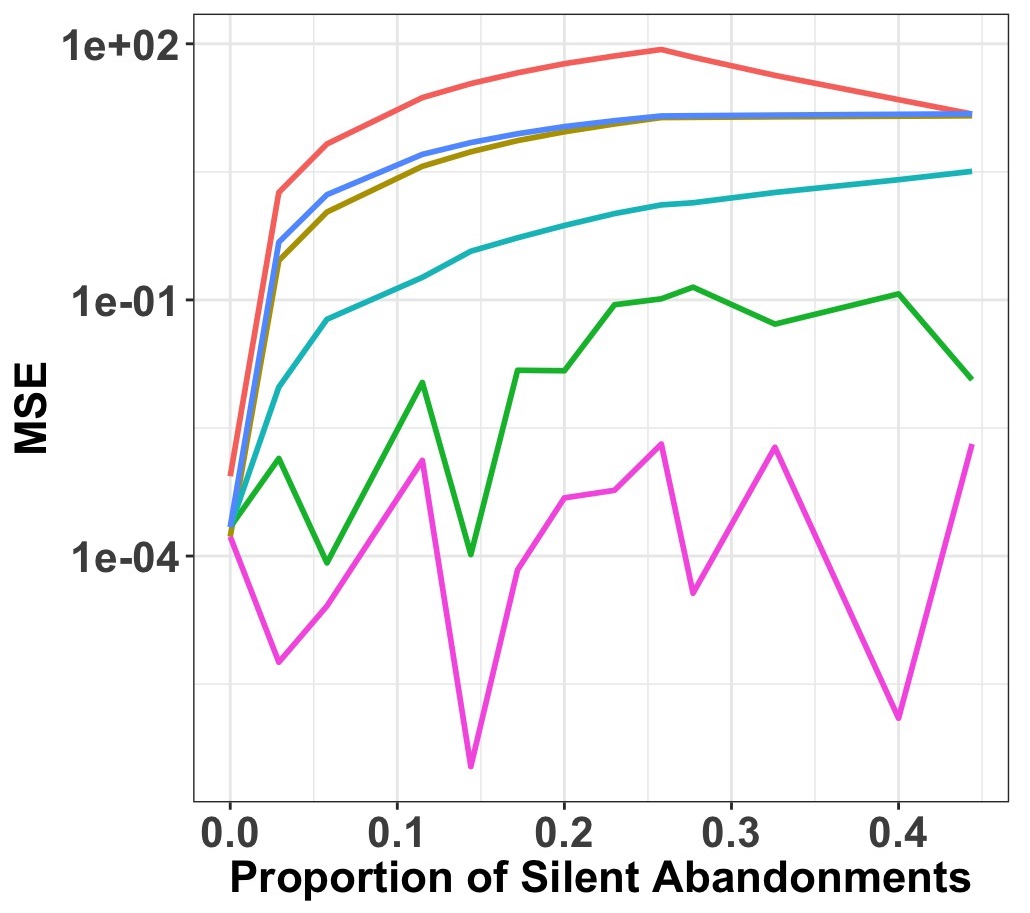
(a) MSE

(b) MSE Ratio (Baseline of the EM Algorithm)

Figure 3: Comparison of Accuracy of Customer Patience Estimations (Log Scale)

Figure 3(a) shows that the errors of the EM are quite small (less than 0.2%) in all of the parameter combinations. Figure 3(b) shows that both ways of implementing Method 1 (which accounts only for right-censored data) are very inaccurate. Specifically, estimating customer patience while ignoring the silent-abandonment phenomenon altogether results in an error rate that is $O(10^{8})$ higher than the error rate in the EM baseline. A similar picture emerges when implementing Method 2, which assumes that all the uncertain conversations as served. Here too the error rate is $O(10^{8})$ higher than the error rate in the EM. If we take silent-abandonment conversations into account to the extent that we regard them as left-censored conversations but ignore the missing data we obtain a (relatively) lower error rate. This is apparent when we look at the other two ways of implementing Method 2: either by considering all missing data to be silent-abandonment conversations or by completing the data with an SVM model. The problem with the latter approach is that the classification is considered correct, whereas a classification model is not completely accurate but has certain sensitivity and specificity proportions. However, both of the above-mentioned options yield less accurate results than the EM: the respective error rates are $O(10^{5})$ and $O(10^{7})$ greater than the error rate of the EM. To conclude, our algorithm outperforms all other methods for estimating customer patience. Note that when there is no silent abandonment in the system (0% in Figure 3), all methods achieve the same performance level; this suggests that the EM algorithm can be used also in cases where the company does not have Sab customers or is unsure whether they exist. Accuracy results for $q$ and $\gamma$ are presented in Appendix 9.1. Our algorithm provides an accurate estimation of $\gamma$ and $q$ too. Since $q$ is a unique feature of our algorithm, we include there only an MSE graph without comparison to other methods.

(a) 2% Sab ($\theta=4$, $\gamma=10$, $q=0.9$)

(b) 17% Sab ($\theta=4$, $\gamma=10$, $q=0.4$)

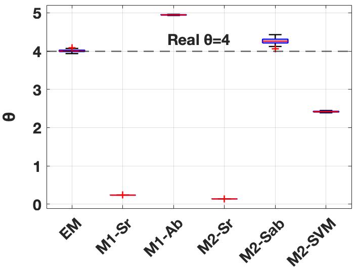
(c) 40% Sab ($\theta=4$, $\gamma=5$, $q=0.1$)

Figure 4: Accuracy of Customer Patience Estimations for Low, Moderate, and High Sab Proportions

In order to analyze whether the estimations are biased or just have larger variance, we present the boxplots in Figure 4. Due to space constraints, we include boxplots only for three of the parameter combinations we simulated. The parameters were chosen to enable comparison of estimations of parameters that result in low (2%), moderate (17%), and high (40%) levels of silent abandonment (the parameters are stated in each figure). We see that regardless of the level of silent abandonment, the EM algorithm produces the most accurate estimation of customer patience, followed by Method 2 taking uSab as Sab (M2-Sab), which overestimates $\theta$ (underestimates average customer patience).

4.2.2 Sensitivity analysis.

The next tests are designed to investigate the sensitivity of the EM algorithm under the initiation conditions. In addition, we would like to know whether starting the algorithm under some sophisticated initial conditions, for example, by using a classification model, such as the one we developed in Section 3.2, helps the model to converge to a more accurate estimation. Accordingly, we first investigate the sensitivity of the EM to $\hat{\pi_{i}}$. Note that by Algorithm 1, $\hat{\pi_{i}}$ affects $\widehat{C_{3,0}^{i}}$ and $\widehat{C_{1,0}^{i}}$ only for the class of uSab customers since the data classes of known-abandonment customers and served customers is complete.

We generated 200 samples of 2,000 customer conversations, with the following parameters: $\theta=4,\gamma=10$, and $q=0.5$. For each sample we estimate the parameters ($\widehat{\theta},\widehat{q}$, $\widehat{\gamma}$) using the EM algorithm (with 100 repetitions), and consider the average of those parameters as the final estimator for that sample. We present here four variants for the starting weights, for all the conversations for which $M^{i}=0$.

• Setting all $M^{i}=0$ conversations to be silent-abandonment conversations with probability 1. Formally, $\widehat{C_{3,0}^{i}}=1$ and $\widehat{C_{1,0}^{i}}=0$ for all conversations with $M^{i}=0$.

• Setting all $M^{i}=0$ conversations to be short-service conversations with probability 1. Formally, $\widehat{C_{3,0}^{i}}=0$ and $\widehat{C_{1,0}^{i}}=1$ for all conversations with $M^{i}=0$.

• Setting 50% of the conversations to be short-service conversations and 50% to be Sab conversations, i.e., for 50% of the conversations with $M^{i}=0$ we set $\widehat{C_{3,0}^{i}}=1$ and for the rest of $M^{i}=0$ we set $\widehat{C_{1,0}^{i}}=1$. We choose this option because within our data about 50% of the conversations are Sab and about 50% are short service (see §3).

• For conversations with $M^{i}=0$, we simulate a classification with sensitivity and specificity proportions according to our best classification model from Section 3; therefore, 85% of the Sab conversations are classified correctly and 76% of the short-service conversations are classified correctly. That is, 85% of the actual $C_{3}=1$ are identified as such and 76% of the actual $C_{1}=1$ are identified as such and, therefore, we set the correct values to $\widehat{C_{3,0}^{i}}$ and $\widehat{C_{1,0}^{i}}$. For the remainder of the conversations we set wrong values on $\widehat{C_{3,0}^{i}}=1$ and $\widehat{C_{1,0}^{i}}=1$; e.g., for an actual $C_{3}=1$: $\widehat{C_{3,0}^{i}}=0$, $\widehat{C_{1,0}^{i}}=1$.

Figure 5: Sensibility Analysis (Setting: $\theta=4$)

Figure 5 shows that the estimations of customer patience are stable and do not change when different initial values are inserted in the EM algorithm.This suggests that one may not need to use the output of the classification model we developed in Section 3 (or any model with similar sensitivity and specificity proportions) as starting probabilities in the EM algorithm. Appendix 9.2 presents the same type of analysis of the sensitivity of the EM algorithm under the initiation conditions when estimating $q$ and $\gamma$. We show there that these estimations are not sensitive to the starting weights either.

4.2.3 Real messaging system data and robustness.

All previous tests used simulated data that clearly adhered to our model assumptions. In this section we perform tests that rely on real data that may not adhere to those assumptions. This will provide us with greater confidence in applying the method we developed here in practice. Using the messaging contact center dataset described in Section 2, we compare the same six methods for estimating customer patience as in the previous accuracy test (§4.2.1). The results are presented in Table 4. The differences between the patience estimations are huge (13–188 minutes). Note that the estimations are consistent with previous tests, where Method 1 and Method 2 overestimate and underestimate customer patience depending on the variation of the method.

The main challenge we are confronted with in this comparison is the lack of ground truth, because we do not know the true value of customer patience. We overcome this challenge by using the manually tagged data described in Section 3.2. Since this data is tagged it has complete data on which customers abandoned, allowing us to apply the method of Yefenof et al. (2018). The resulting estimation of customer patience, based on that data, is 81.9 minutes (row 1 of Table 4). This is very similar to the EM algorithm estimation of customer patience that is based on the monthly data: 81.11 minutes (row 6 of Table 4). On the other hand, it is very far from the estimations done using the other methods. Therefore, we can conclude that the EM algorithm (Algorithm 1) is able to cope with the missing data and obtains an accurate estimation of customer patience.

Going back to Table 4, we notice the large bias missing data generates in the estimations. When we ignore both silent abandonment and missing data by regarding all uncertain silent abandonment ($M=0$) as service ($C_{1}$=1) and by estimating customer patience using either Method 1 or Method 2, we overestimate patience by twice or more (rows 2 and 3 of Table 4). Note that this is the current practice of many companies. They use Method 1 (row 2) while ignoring the concept of silent abandonment that creates left-censoring and missing data. A more advanced company may have a better understanding of its system and an awareness of silent abandonment. However, if it is still unaware of the existence of missing data, it will consider all of the conversations in class $M=0$ to be silent-abandonment conversations ($C_{3}=1$) and apply either Method 1 (i.e., and ignore left-censoring) or Method 2 (i.e., and not ignore the left-censoring). In both cases it underestimates customer willingness to wait (rows 4 and 5).

One might comment on our finding that the customers in messaging systems are willing to wait for more than 1 hour (row 1 of Table 4). We think such enduring patience is reasonable for three reasons. (a) When reading the content of the conversations, we saw that in this particular contact center customers receive an automatic message instructing them to “go on with their daily activities” (while waiting for a reply) and to address the service as if “talking to a friend.” These customers therefore expect longer waits and adjust their patience accordingly. (b) Messaging systems are used to support the continuance of the relationship between customers and companies. As a result, they have a high proportion of returning customers that are expected to have realistic expectations of the virtual wait time, which was found to be 8.77 minutes. The fact that customer patience outlasts the virtual wait time is consistent with similar results from call centers (Brown et al. 2005). (c) Mandelbaum and Zeltyn (2013) showed that customers are willing to wait around 2 (or more) times longer than their service requirement. Recall that here service time is 49.2 minutes, which fits our findings well.

A potential problem with EM algorithms is that they might converge to a saddle point (Chapter 8 of Little and Rubin 2002). To verify that this does not happen here, we started our EM algorithm with different weights. Specifically, we estimated the parameters by using the EM and taking the starting weights $\widehat{C_{3,0}^{i}}$ for the conversations for which $M^{i}=0$ to be $1$, $0$, $.5$, or $\hat{\pi_{i}}$ from the SVM model, as in Section 4.2.2. Note that in the last case the classification model is not simulated; it is the real SVM presented in Section 3. In every case the obtained parameters ($\widehat{\theta},\widehat{q}$, $\widehat{\gamma}$) were consistent, verifying that the algorithm did not converge to a saddle point when applied to the real messaging data.

Table 4: Comparison of Estimations of Average Customer Patience: Messaging System Dataset (May 2017)

Row	Method	Average Patience (Minutes)
1	Method 2—Using sample of labeled conversations	81.90
2	Method 1—Uncertain silent abandonment is service	166.42
3	Method 2—Uncertain silent abandonment is service	188.07
4	Method 1—Uncertain silent abandonment is abandonment	28.27
5	Method 2—Uncertain silent abandonment is silent abandonment	13.17
6	EM	81.11

Finally, we performed several robustness checks, by dividing the data set into 10–15 samples and estimating patience in each one of them, using the EM 100 times. We performed these tests to make sure that the results that we obtained from the monthly data ($\hat{\theta}=0.739$, $\hat{q}=0.58$, and $\hat{\gamma}=6.78$) are robust. We find that the estimations of $\theta$ from subsamples of the dataset are consistent with those of the whole dataset corpus (Figure 6). We present our results for the estimations of $q$ and $\gamma$ in Appendix 9.3, which are as accurate.

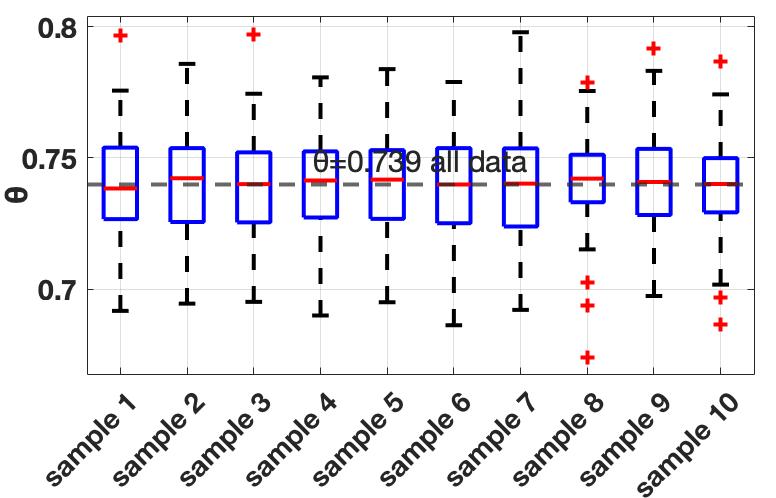
Figure 6: Estimations of the Parameter of Customer Patience ($\theta$) using EM Algorithm in Subsamples of the Messaging Dataset (May 2017). Horizontal Line Indicates Estimation Based on the Entire Dataset $\hat{\theta}=0.739$

In Appendix 9.4 we provide a final validation in a more realistic setting, with the help of a simulated queueing model with parameters from real data. In this setting the assumptions of the EM algorithm (Assumption 4.1) may not necessarily be true. We find that in this setting too the EM estimation of $\theta$ is the most accurate among the compared methods. We also find that the differences with the other methods are more pronounced than with the previous validations in the present section. Additionally, we find that the EM estimations of $q$ and $\gamma$ are also the most accurate among the compared methods.

5 Incorporating Silent Abandonment into a Queueing Model and Managerial Implications

In this section we analyze how the phenomenon of silent abandonment affects system efficiency and what decision-makers can do about it. As explained, silent abandonment affects system efficiency in two ways: (a) the Sab customer holds a service slot within the concurrency system, preventing other customers from entering service while idling the agent who is waiting for the customer’s response. (b) The agent may waste time on solving the no longer relevant problem of the Sab customer. Both forms of system inefficiency reduce the system’s capacity in high-load moments, when available capacity is most crucial. In our chat and messaging system datasets, system capacity is reduced by 5% and 11%, respectively. According to queueing theory, such a reduction in agent availability should have a huge impact on system performance in overloaded systems (Koole and Mandelbaum 2002). The aims of the present section are as follows. First, we introduce a queueing model that takes the Sab phenomenon into account. Then we show that such a queueing model is able to predict contact-center performance measures better than models that neglect to account for silent abandonment. Finally, we use the model to analyze how much the loss of capacity due to Sab harms system performance, and discuss several ways one might avoid such a problem.

We propose the queueing model presented in Figure 7 to capture the phenomenon of silent abandonment. We assume that the arrival rate is according to a Poisson process with rate $\lambda$. Customers entering the queue have finite patience that is exponentially distributed at rate $\theta$. The probability that an abandoning customer will indicate her abandonment is denoted by $q$. Customers who don’t provide that indication stay in the queue and are assigned to a service agent (when one becomes available). Queueing policy is first-come, first-served (FCFS). The company can provide service to $n$ customers in parallel; i.e., there are $n$ service slots of statistically identical agents. Service time is exponentially distributed with rate $\mu_{Sr}$ for served customers (i.e., those who belong to class $C_{1}$) and rate $\mu_{Sab}$ for Sab customers (i.e., those who belong to class $C_{3}$). This model is very similar to the Erlang-A (M/M/N+M) model, with the important difference that a customer that abandons the queue, but does not notify the system of her abandonment, is assumed by the system to be in the queue (e.g., the gray customer in Figure 7) and, when assigned to an agent, receives some service time, albeit at a different service rate. This enables us to capture the loss of capacity that results from Sab customers.

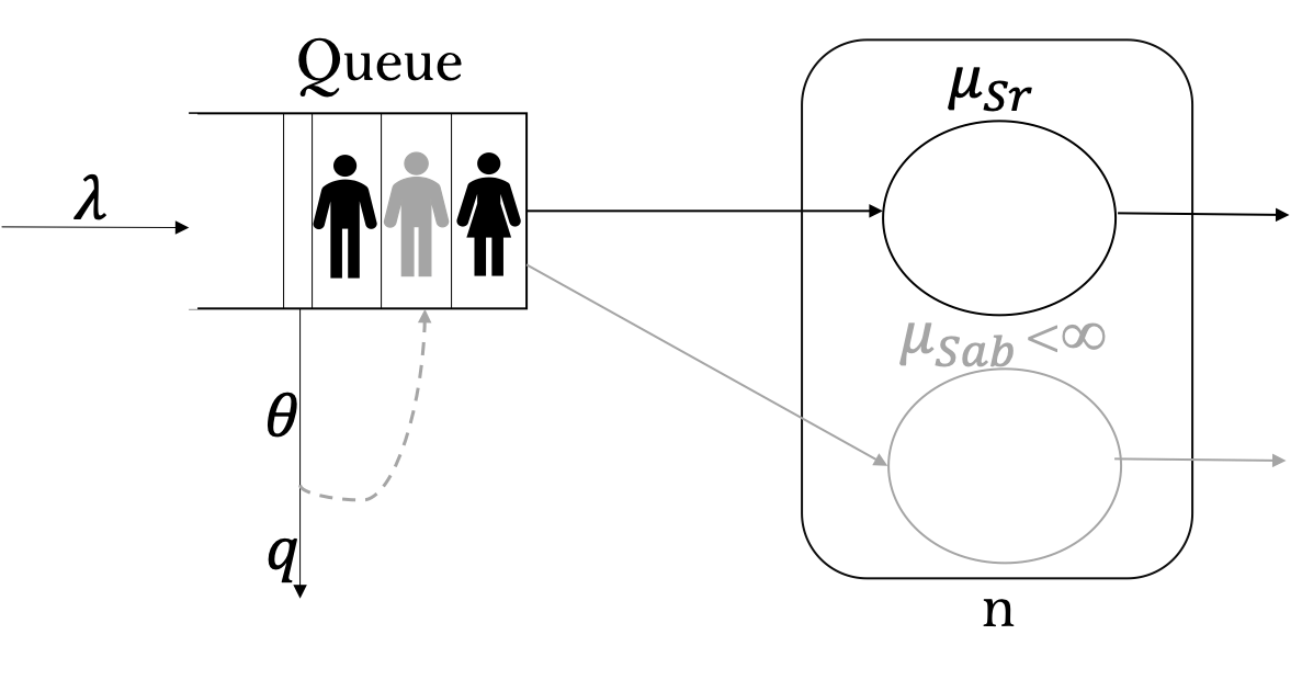
Figure 7: Queueing Model with Silent Abandonment

To verify that this queueing model is of merit, we fit the model to the chat system dataset described in Section 2.1. The Erlang-A (M/M/N+M) model which takes into account Kab customers (Palm 1957, Mandelbaum and Zeltyn 2007) is used as a baseline. We then test new models by gradually adding features of silent abandonment. We consider the following five variants of fitting a queueing model to the chat dataset:

• An Erlang-A queueing model that ignores Sab both in the queue dynamics and in the parametric estimation of customer patience. Labeled as “(1) Ignoring Sab.”

• An Erlang-A queueing model that ignores Sab in the queue dynamics, but considers it in the parametric estimation of customer patience. Labeled as “(2) Considering Sab as Kab”.

• A queueing model with Sab, no loss of capacity due to Sab, and that considers Sab in the estimation of customer patience, i.e., the model in Figure 7 with $\mu_{Sab}=\infty$. We check two versions of this model: one with a nonparametric estimation of customer patience (Model (3)) and the other with a parametric estimation of customer patience (Model (4)). Labeled as “(3) Sab as left-censored, nonparametric” and “(4) Sab as left-censored, parametric,” respectively.

• A queueing model with Sab, loss of capacity due to Sab, and that considers Sab in the parametric estimation of customer patience, i.e., the model in Figure 7. Labeled as “(5) Considering Sab as time-consuming.”

In Model (1) we estimate customer patience based on Mandelbaum and Zeltyn (2013) (Method 1), and the service rate is calculated by averaging the service time of all the customers that were assigned to an agent, regardless of whether they were served or silently abandoned the queue. In Model (2) we estimate customer patience based on Method 1 as well, and the service rate is estimated only for served customers ($C_{1}=1$), i.e., $\mu=\mu_{Sr}$. In Models (3) and (4) we estimate customer patience based on Yefenof et al. (2018) (Method 2). In both models service time is calculated only for served customers. Finally, in Model (5) we estimate customer patience based on Yefenof et al. (2018) (Method 2). Service time is calculated separately for served customers and Sab customers. (Note that using the EM in the case of Models (4) and (5) gives the same customer patience estimation.)

Table 5 provides the estimations of customer patience from real chat data used in this section. This dataset has complete data, which is consistent with the assumption of both versions of Method 2 (rows 3 and 4). We will show next, with the help of our simulation experiments which estimator works better.

Table 5: Comparison of Estimations of Average Customer Patience: Chat System Dataset (February 2017)

Row	Method	Average Patience (Minutes)
1	Method 1—Ignoring Sab	33.9
2	Method 1—Considering Sab as Kab	17.1
3	Method 2—Sab as left-censored, nonparametric	7.8
4	Method 2—Sab as left-censored, parametric	2.0

We compared the differences between the simulated performance measures of the five queueing models described above and the real performance measures calculated from the dataset (shown in Appendix 10). Table 6 presents the differences using the root mean square error (RMSE) score. The simulation parameters $\lambda_{t}$, $\mu_{t}$, and $n_{t}$ were estimated for each hour over the month, while the parameters of customer patience distribution were kept constant over time. The parameters $\theta$ and $\mu_{t}$ were estimated differently for each model according to the description above. Note that $n_{t}$ is the number of available slots, i.e., the number of online agents times a fixed concurrency level of 3 customers per agent. (As mentioned in Section 2.1, the concurrency level is the maximal number of customers that can be served in parallel, such that if all the slots are occupied and an additional customer enters the system, she will need to wait in the queue.)

Table 6: RMSE between Queueing Models and Chat System Dataset (February 2017)

Performance	(1) Ignoring	(2) Considering	(3) Sab as left-censored	(4) Sab as left-censored	(5) Considering Sab as
Measure	Sab	Sab as Kab	nonparametric	parametric	time-consuming
$P\{\text{Wait}>0\}$	0.27	0.26	0.28	0.31	0.27
$P\{\text{Ab}\}$	0.12	0.11	0.09	0.08	0.07
E[Queue]	3.27	1.68	1.18	0.96	0.87
E[Wait]	169.56	85.13	75.69	70.29	63.44
E[Wait$|$Served]	198.29	103.04	83.63	63.44	62.47

Model (1) (in Table 6) was designed to provide a baseline of the fit between the model and the data when the phenomenon of silent abandonment is ignored altogether. We see that the fit of the queueing model to the data in this case is the worst among all the compared models. Model (2) is designed to represent a case where the company acknowledges the presence of Sab customers, but does not deal with them correctly when estimating customer patience. That is, instead of understanding that they represent left-censored data, they simply consider them as Kab occurring before the assignment time. We see that this strategy is too simplistic, and yields a poor fit of the queueing model to the data. In Models (3) and (4) the company understands that silent abandonment occurs and that the data is left-censored, but ignores the impact of Sab on the available capacity. By comparing the two versions we note that the fit of the parametric model to the data is much better than that of the nonparametric model. This give us higher confidence that the assumptions we made in Assumption 4.1 are actually very reasonable for the contact-center environment. Finally, we observe that Model (5) which considers Sab both in terms of patience estimation and in terms of efficiency loss, is the best fit, emphasizing the importance of taking the phenomenon of silent abandonment into account when modeling contact centers.

Figure 8(a) presents a comparison of the estimation of E[Wait] for Models (4) and (5), and the real E[Wait] in the dataset of the chat system, as a function of the hour of the day (with 95% confidence intervals). We clearly see that Model (4) underestimates customers’ wait time relative to Model (5). Comparing Models (4) and (5) enables us to understand the impact of the capacity loss, caused by the Sab customers, on performance measures. If the company is able to eliminate all capacity loss (5% in our case), the expected wait time of all customers would be reduced by 1.6 minutes (67% in absolute percentage), the expected wait time of served customers would be reduced by 1.5 minutes (83%), the probability of waiting by 3% (8%), the probability of abandonment by 4% (16%), and the expected number of people waiting in queue—E[Queue]—by 0.16 (21%). Figure 8(b) illustrates what happens if this capacity loss is partially reduced. To create this figure we simulated Model (5) with various LOS of Sab customers ($1/\mu_{Sab}$); as $1/\mu_{Sab}$ increases it takes more time to understand that the Sab customer indeed abandoned the queue. For this graph we use the parameters on a typical Monday (13:00–14:00), where $\lambda=56$ customers per hour, LOS of served customers is $12.3$ minutes, $q=0.7$, and average patience is 2 minutes ($\theta=30$ customers per hour). The case where LOS of Sab is 0 is in fact Model (4), and the highest LOS value of Sab (5.6 minutes) resembles Model (5).

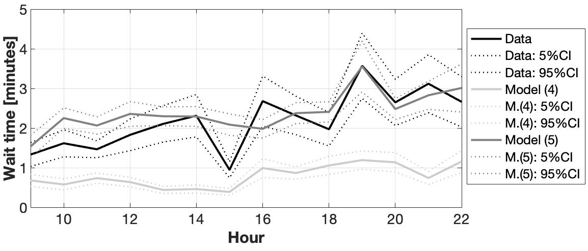
(a) As a Function of Time (Models (4) and (5) and Real)

(b) As a Function of $\mu_{Sab}$ (Models (4)–(5))

Figure 8: Estimations of E[Wait]

How can the company eliminate capacity loss? The first way is to design a bot that is able to identify cases of silent abandonment without the involvement of an agent. Such a bot can manage the beginning of the interaction automatically and transfer the conversation to the agent only after the customer reacts. In chat systems (where the customer does not write anything before joining the queue) such a bot can manage the initiation stages of the chat, namely, the introduction and an inquiry about the customer’s problem. In messaging systems (in which the customer writes an inquiry before joining the queue) the bot can ask whether the customer’s inquiry is still relevant. As some customers might find such a question annoying, the bot can be programmed to use that method only for suspected Sab customers.

To identify suspected Sab customers, the company can design a prediction model in the spirit of the classification model we presented in Section 3, where information about customers’ wait time, class, and initial messages is used to identify Sab customers. As all classification models have some margin of error, even the best such system will assign some Sab customers to agents and waste agent time, but hopefully to a lesser extent than before.

Another way to reduce capacity loss is for the system, when computing agent concurrency levels, to consider suspected Sab customers as fractional customers (as opposed to full ones) until they write something. For example, as long as a customer writes nothing she will be considered a suspected Sab customer and be assigned a value of 0.5, but as soon as she writes something she will be assigned a value of 1. Therefore, an agent that has 2 suspected Sab customers and 2 in-service ones is equivalent to an agent that handles 3 customers. This will reduce the amount of blocking that Sab customers impose on the other customers in the queue.

A final possible solution is to handle queue priorities according to existing information on suspected Sab customers. For example, the bot can send a suspected Sab customer to the end of the queue. Therefore, when the Sab customer’s turn for service arrives, the agent will have reached his idle period, which means that the effect of the Sab customer on system performance would be diminished. We think that this solution is appropriate mostly for customers who enter the queue when the contact center is closed (e.g., at night) and who would be loading the agent’s capacity at the beginning of the workday without actually being there, thereby delaying the new arrivals significantly. In such a scenario, the “cost” imposed by this unfair policy of requiring suspected Sab customers to wait for one extra busy period may be worth it.

6 Discussion

In this article we identified and defined the phenomenon of silent abandonment as an important source of uncertainty in contact centers. Our work exposed and analyzed how a small difference in the service process of two environments of contact centers—chat systems and messaging systems—changes the way we estimate performance and patience for each one. Specifically, we showed that the timing of the submission of a customer’s inquiry (i.e., before entering the queue or after being assigned to an agent) and the customer’s management of her service window/application create uncertainty that affects a company’s ability to know which customers have abandoned the queue and which have been served. We argued that although enabling/denying customer messages before entering the queue is a design decision of the company, the fact that not all people close their application or are impolite (i.e., abandoning without indication) is a behavioral phenomenon that the company cannot control, but needs to deal with.

We further analyzed the impact of silent abandonment on estimations of customer patience and abandonment estimations. We showed that silent abandonment needs to be considered as left-censored observations of customer patience and as time-consuming tasks in order to obtain more accurate measures of performance in contact centers. We suggested a queueing model that takes Sab customers into account, and showed that it captures system dynamics well, whereas queueing models that ignore Sab customers do not fit the data. Using our queueing model we showed the impact of capacity loss, caused by customer behavior, on performance measures. We then made several suggestions for operational changes in concurrency management and prioritization to avoid that problem. We are in the process of analytically analyzing this queueing model. We believe that it can be used as a tool to evaluate further the operational implications of silent abandonment, as well as a tool to validate recommendations of new operational policies that will be able to cope better with those implications.

When comparing customer patience in chat and messaging systems, we notice a huge difference. The EM algorithm estimated customer patience in the messaging system to be 81.1 minutes and customer patience in the chat system to be much shorter, only 2 minutes. The higher patience in the messaging system is consistent with previous literature that shows a connection between customer LOS and willingness to wait; e.g., in Mandelbaum and Zeltyn (2013), customer LOS in the messaging system is much longer than in the chat system, 49.2 and 11.65 minutes, respectively. Even so, patience in chat systems seems short. We conjecture that the difference in customer patience between the two contact-center environments is related to the different nature of the service in those systems. In the messaging system, the communication is usually through a smart phone, which are always with us, whereas, in the chat system, the communication is usually through a desktop computer, which obligates us to remain stationary. This conjecture relates to the work of Westphal (2018) who shows that a customer is more likely to abandon the queue when waiting for an online service when forced to focus on a waiting screen on a computer than when waiting for an online service when free to shift attention to other websites.

When analyzing the total percentage of abandoning customers in both environments we see that it is almost the same, around 20%. However, the percentage of Sab customers is higher in the messaging system, where the wait is longer too. This is somewhat similar to the increase in the no-show rate as the wait time from appointment booking to physician visit increases (Folkins et al. 1980, Galucci et al. 2005, Liu et al. 2010). The authors of the first of these articles claim that in the setting of a mental health center, it may be the case that no-shows happen due to customers having to wait longer solve their problems on their own. We conjecture that this may also be true for textual services. This raises the question whether there is a connection between $q$ and wait time. We therefore think that future research on patience estimation can relax the assumptions we made for the EM algorithm on the independence between $q$ and wait time.

Another interesting comparison can be made between silent abandonment and no-shows vis-à-vis the scope of these phenomena and their operational implications. Our findings suggest that 6%–14.3% of the customers abandon queues of contact centers without notification, compared to 23%–34% of no-shows in medical appointments. In terms of operational implications, Moore et al. (2001) found that in a family medical practice no-shows are responsible for 25.4% of scheduled wasted time. Here too we showed that silent abandonment reduces system capacity, but at a lower magnitude of 5%–11%. However, here it translates to wasted tasks performed by the agent and occupied slots held by the silent-abandonment customers in the system.

From a different perspective we note that agents may use the silent-abandonment phenomenon to their advantage. If a Sab customer is assigned to an agent, the agent seems to be busy while in practice she may rest a little. Therefore, agents may lack incentive to close suspected Sab conversations quickly. The company will want to prevent such strategic behavior by agents, but should proceed carefully in order to avoid situations where a long-waiting customer conversation is prematurely terminated. For example, it is possible that the customer did not notice that the agent finally answered. Hence, finding technological answers to handling capacity loss, like the ones we suggested in Section 5, is important. Investigating the strategic behavior of agents may be interesting in its own right and a worthy topic of future research.

To conclude, we believe that the phenomenon of silent abandonment has an impact beyond the framework discussed in this paper, and therefore calls for further mathematical and behavioral modeling in the context of chat- and messaging-based services.

7 Classification models

We provide here details on the two best classification models described in Section 3: the SVM model and the classification tree.

7.1 Support vector machines

The fitted model has 259 support vectors. Significant variables included in this model are:

1. AgentChars: the number of characters written by the agent in the conversation.

2. AgentDuration: the time it takes the agent to write her messages.

3. QueueTime: the time the customer waits for agent assignment in the queue.

4. TotalDuration: the time from agent assignment until manual closure of the conversation by the agent or automatically by the system.

5. wordag46, wordag1, wordag20, wordag31: specific words written by the agent during the conversation. (We provide only coded words due to privacy concerns of the company providing the dataset.)

6. wordcust1: a specific word written by the customer in her initial inquiry.

7.2 Classification tree

The fitted classification tree is presented in Figure 9. Significant variables included in this model are:

1. AgentChars, AgentDuration, QueueTime, TotalDuration, wordag46: see 7.1

2. SessionStartHour: the hour that the customer arrived to the system.

3. SessionStartDayofWeek: the day of the week on which the customer arrived to the system.

4. InnerWait: the time the customer waits for the agent’s reply during service (i.e., after assignment to the agent).

5. SessionEndHour: the hour that the conversation was closed; the conversation may be closed manually by the agent (usually within a few hours of no customer reply) or automatically by the system (after a threshold time has passed).

6. SessionEndDayofWeek: the day of the week on which the conversation is closed.

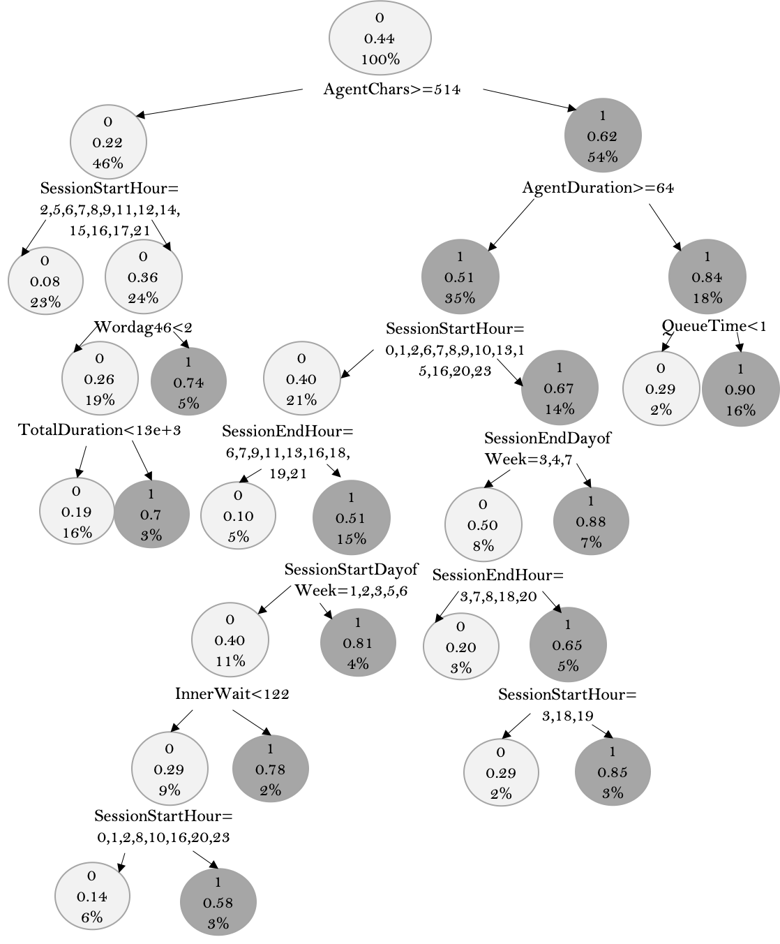
Figure 9: Classification Tree for the Probability of a Conversation Being a Silent Abandonment. Splitting Variable on the Bottom of the Nodes. Nodes Show 1 for Silent Abandonment (Grey) and 0 for Short Service (Light Grey); Probability of Obtaining that Classification; Percentage of the Data that Falls into That Node.

8 EM Algorithm: Proof and Explanation

The log of the likelihood in Eq. (2) is

$$\begin{split}l(D,\theta,q,\gamma)=\sum_{i=1}^{n}\left\{\left(1-\Delta_{i}\right)\left(\log\gamma-\gamma U_{i}-\theta U_{i}\right)\right\}+\sum_{i=1}^{n}\left\{\left(\Delta_{i}Y_{i}\right)\left[\log\theta-\theta U_{i}-\gamma U_{i}+\log(q)\right]\right\}\\ +\sum_{i=1}^{n}\left\{\left(\Delta_{i}(1-Y_{i})\right)\left[\log(1-q)+\log(1-e^{-\theta U_{i}})+\log\gamma-\gamma U_{i}\right]\right\},\end{split}$$ (7)

where, if the data is complete, the possible classes for conversation $i$ are $C_{1}^{i}=1-\Delta_{i}$, $C_{2}^{i}=Y_{i}\Delta_{i}$, and $C_{3}^{i}=(1-Y_{i})\Delta_{i}$. Therefore, the log-likelihood in Eq. (7) when the data is complete can be written as

$$\begin{split}l(D,\theta,q,\gamma)=\sum_{i=1}^{n}\left\{\left(C_{1}^{i}\right)\left(\log\gamma-\gamma U_{i}-\theta U_{i}\right)\right\}+\sum_{i=1}^{n}\left\{\left(C_{2}^{i}\right)\left[\log\theta-\theta U_{i}-\gamma U_{i}+\log(q)\right]\right\}\\ +\sum_{i=1}^{n}\left\{\left(C_{3}^{i})\right)\left[\log(1-q)+\log(1-e^{-\theta U_{i}})+\log\gamma-\gamma U_{i}\right]\right\}.\end{split}$$ (8)

In the case of missing data in $\Delta$ we cannot maximize the log-likelihood in Equation (8) because some of the observations might belong to class $C_{1}=1$ or $C_{3}=1$. To solve this problem we use the expectation-maximization (EM) algorithm. It calculates starting parameters with random starting weights for conversation classes (see Algorithm 1) and then iterates between two steps—the expectation and the maximization steps—until convergence. (The convergence criterion is given in Algorithm 1.)

8.1 Expectation Step, Proof of Theorem 4.1

In the $t$th iteration the expectation step consists of finding a surrogate function that is a lower bound on the log-likelihood in Eq. (8) but is tangent to the log-likelihood at $(\widehat{\theta^{(t)}},\widehat{q^{(t)}},\widehat{\gamma^{(t)}})$, the vector of the parameters of the latest iteration, $t-1$. We achieve this by computing the expectation given what we know up to the $t$th iteration, i.e. the $t-1$th estimations of the parameters $(\widehat{\theta^{(t)}},\widehat{q^{(t)}},\widehat{\gamma^{(t)}})$ and the data that is complete. Formally,

$$E\left[l(D,\theta,\gamma,q)\mid U_{i},M^{i},\widehat{\theta^{(t)}},\widehat{\gamma^{(t)}},\widehat{q^{(t)}}\right],$$ (9)

where $M$ is defined as in 4.1.2.

When $M^{i}=2$ the data is complete, implying that for that conversation $C^{i}_{2}=1$. Therefore, we can compute (9) for such $i$th observations as follows:

$$E\left[C_{2}^{i}=1\mid U_{i},M^{i},\widehat{\theta^{(t)}},\widehat{q^{(t)}},\widehat{\gamma^{(t)}}\right]=E\left[\Delta_{i}Y_{i}\mid U_{i},M^{i},\widehat{\theta^{(t)}},\widehat{q^{(t)}},\widehat{\gamma^{(t)}}\right] =1_{\{M^{i}=2\}}+\left(0\right)\left(1_{\{M^{i}\neq 2\}}\right).$$

We define $\widehat{C_{2,t}^{i}}$ as the probability that the $i$th conversation is a known abandonment in the $t$th iteration. This is exactly what the previous function represents. Therefore,

$$\widehat{C_{2,t}^{i}}=1_{\{M^{i}=2\}}.$$

When $M^{i}=0$ there is missing data. This implies that for conversation $i$ either $C^{i}_{1}=1$ or $C^{i}_{3}=1$. We first compute Eq. (9) by conditioning on knowing that the $i$th observation is a member of class $C_{3}=1$:

$$E\left[C_{3}^{i}=1\mid U_{i},M^{i},\widehat{\theta^{(t)}},\widehat{q^{(t)}},\widehat{\gamma^{(t)}}\right] =E\left[\Delta_{i}\left(1-Y_{i}\right)\mid U_{i},M^{i},\widehat{\theta^{(t)}},\widehat{q^{(t)}},\widehat{\gamma^{(t)}}\right]$$

$$=\left(1_{\{M_{i}=0\}}\right)Pr\left\{\Delta_{i}=1\mid U_{i},M^{i}=0,\widehat{\theta^{(t)}},\widehat{q^{(t)}},\widehat{\gamma^{(t)}}\right\}+\left(0\right)\left(1_{\{M_{i}\neq 0\}}\right)$$

$$=\left(1_{\{M_{i}=0\}}\right)Pr\left\{T_{i}\leq W_{i}\mid U_{i}=W_{i},\widehat{\theta^{(t)}},\widehat{\gamma^{(t)}}\right\}$$

$$=\left(1_{\{M_{i}=0\}}\right)Pr\left\{T_{i}\leq U_{i}\mid U_{i},\widehat{\theta^{(t)}}\right\}$$

$$=1_{\{M_{i}=0\}}\left(1-e^{-\widehat{\theta^{(t)}}U_{i}}\right).$$

The first equality follows since a customer $i$ for which $M^{i}=0$ does not give an indicator when abandoning the queue, i.e., $Y_{i}=0$, and by the independence of $\Delta_{i}$ and $Y_{i}$. The second equality follows since for a customer $i$ that belongs to class $C_{3}=1$ must have $M^{i}=0$ and clearly they are customers that abandoned. Hence, by definition $\Delta_{i}=1$, which formally means that $T_{i}\leq W_{i}$. Additionally, when $M^{i}=0$, the observed time $U_{i}$ is their wait time $W_{i}$; hence, the third equality follows. The fourth equality is implied from the third. The fifth equality follows since the fourth equality represents the cdf $F$ of patience time $T$ that has an exponential distribution by Assumption 4.1.

We define $\widehat{C_{3,t}^{i}}$ as the estimated probability that an $i$ customer is a silent abandonment in the $t$th iteration, which by the above calculation is

$$\widehat{C_{3,t}^{i}}=1_{\{M^{i}=0\}}\left(1-e^{-\widehat{\theta^{(t)}}U_{i}}\right).$$

Note that in the case where $M^{i}=0$ for conversation $i$, we need to consider also that the customer might belong to $C_{1}^{i}=1$. In addition, we have another group that belongs to class $C_{1}=1$, namely, the conversations where $M=1$. For them the data is complete. So the computation of Eq. (9) for an $i$ customer that belongs to class $C_{1}^{i}=1$ is as follows:

$$E\left[C_{1}^{i}=1\mid U_{i},M^{i},\widehat{\theta^{(t)}},\widehat{q^{(t)}},\widehat{\gamma^{(t)}}\right] =E\left[1-\Delta_{i}\mid U_{i},M^{i},\widehat{\theta^{(t)}},\widehat{q^{(t)}},\widehat{\gamma^{(t)}}\right]$$

$$=\left(1_{\{M^{i}=0\}}\right)Pr\left\{\Delta_{i}=0\mid U_{i},M^{i}=0,\widehat{\theta^{(t)}},\widehat{q^{(t)}},\widehat{\gamma^{(t)}}\right\}+1_{\{M^{i}=1\}}$$

$$=\left(1-\widehat{C_{3,t}^{i}}\right)1_{\{M^{i}=0\}}+1_{\{M^{i}=1\}}.$$

The second term on the right-hand side of the second equality ($1_{\{M^{i}=1\}}$) follows since for the customers that are classified as $M=1$ the data is complete. The first term follows since some of the customers in $M=0$ belong as well to $C_{1}=1$ and these customers are the ones who do not abandon, i.e., $\Delta=0$. The third equality follows since the probability of a customer $i$ in $M^{i}=0$ being served (not abandoned) is exactly the complement of $\widehat{C_{3,t}^{i}}$.

We define $\widehat{C_{1,t}^{i}}$ as the probability that an $i$ customer is a served customer, which by the above computation is

$$\widehat{C_{1,t}^{i}} =\left(1-\widehat{C_{3,t}^{i}}\right)1_{\{M^{i}=0\}}+1_{\{M^{i}=1\}}.$$

Finally, we can rewrite our log-likelihood, Eq. (7), in the $t$th iteration with missing data as Eq. (3). This is exactly the surrogate function that is a lower bound on the log-likelihood: the E-step in Algorithm 1.

$\blacksquare$

8.2 Maximization Step, Proof of Theorem 4.2

In the $t$th iteration of the maximization step, the parameters $(\widehat{\theta^{(t+1)}},\widehat{q^{(t+1)}},\widehat{\gamma^{(t+1)}})$ are found to be the maximizers of the surrogate function defined in Eq. (7). We obtain the parameters $(\widehat{\theta^{(t+1)}},\widehat{q^{(t+1)}},\widehat{\gamma^{(t+1)}})$, where the partial derivatives of the the surrogate function (3) are equal to zero.

The partial derivative with respect to $q$ is

$$\begin{split}\frac{\partial\ell}{\partial q}&=\end{split}\left(\frac{1}{q}\right)\sum_{i=1}^{n}\widehat{C_{2,t}^{i}}-\left(\frac{1}{1-q}\right)\sum_{i=1}^{n}\widehat{C_{3,t}^{i}},$$

which yields

$$\widehat{q^{(t+1)}}=\left\{\sum_{i=1}^{n}\widehat{C_{2,t}^{i}}\right\}\left\{\sum_{i=1}^{n}\left(1-\widehat{C_{1,t}^{i}}\right)\right\}^{-1}.$$

The partial derivative with respect to $\gamma$ is

$$\frac{\partial\ell}{\partial\gamma}=\frac{1}{\gamma}\sum_{i=1}^{n}\left(1-\widehat{C_{2,t}^{i}}\right)-\sum_{i=1}^{n}U_{i},$$

which yields

$$\widehat{\gamma^{(t+1)}}=\left\{\sum_{i=1}^{n}\left(1-\widehat{C_{2,t}^{i}}\right)\right\}\left\{\sum_{i=1}^{n}U_{i}\right\}^{-1}.$$

The partial derivative with respect to $\theta$ is

$$\frac{\partial\ell}{\partial\theta} =\sum_{i=1}^{n}\left(\widehat{C_{1,t}^{i}}\right)\left(-U_{i}\right)+\sum_{i=1}^{n}\left(\widehat{C_{2,t}^{i}}\right)\left(-U_{i}+\frac{1}{\theta}\right)+\sum_{i=1}^{n}\widehat{C_{3,t}^{i}}\frac{U_{i}e^{-\theta U_{i}}}{1-e^{-\theta U_{i}}}$$

$$=\sum_{i=1}^{n}\left(U_{i}\right)\left(-\widehat{C_{1,t}^{i}}-\widehat{C_{2,t}^{i}}\right)+\sum_{i=1}^{n}\left(\frac{\widehat{C_{2,t}^{i}}}{\theta}\right)+\sum_{i=1}^{n}\widehat{C_{3,t}^{i}}\frac{U_{i}e^{-\theta U_{i}}}{1-e^{-\theta U_{i}}}$$

$$=\sum_{i=1}^{n}\left(U_{i}\right)\left(\widehat{C_{3,t}^{i}}-1\right)+\sum_{i=1}^{n}\left(\frac{\widehat{C_{2,t}^{i}}}{\theta}\right)+\sum_{i=1}^{n}\widehat{C_{3,t}^{i}}\frac{U_{i}e^{-\theta U_{i}}}{1-e^{-\theta U_{i}}}.$$

The second equality follows from simplifying the terms. The third equality follows from the relation $-\widehat{C_{1,t}^{i}}-\widehat{C_{2,t}^{i}}-\widehat{C_{3,t}^{i}}=-1$ for the $i$th customer in the $t$th iteration.

Finally, we set the derivative to zero and multiply by $\widehat{\theta^{(t+1)}}$

$$\widehat{\theta^{(t+1)}}\left\{\sum_{i=1}^{n}\left(\widehat{C_{3,t}^{i}}-1\right)U_{i}\right\}+\sum_{i=1}^{n}\widehat{C_{2,t}^{i}}+\widehat{\theta^{(t+1)}}\left\{\sum_{i=1}^{n}\widehat{C_{3,t}^{i}}\frac{U_{i}e^{-\widehat{\theta^{(t+1)}}U_{i}}}{1-e^{-\widehat{\theta^{(t+1)}}U_{i}}}\right\}=0.$$

$\blacksquare$

9 EM Algorithm Validation

9.1 Accuracy with Regard to the Estimation of $q$ and $\gamma$

In this appendix we provide the MSE of the estimation of $q$ using the simulated data described in Section 4.2.1. Note that here we cannot compare to other methods since only the EM algorithm estimates this parameter. Figure 10(a) presents the MSE of $q$ as a function of the proportion of silent abandonment customers (out of all the arriving customers) in logarithmic scale. We show here that the error rate is very small; therefore, the estimation is very accurate.

Figure 10(b) presents the MSE results for estimating $\gamma$ in a logarithmic scale. The x-axis is the proportion of silent-abandonment customers (out of all the arriving customers). We note that the estimation of most of the methods is exactly the same, except for the method of Mandelbaum and Zeltyn (2013), where we take the uncertain conversations ($M=0$) to be $C_{2}$. For this reason, most of the lines in Figure 10(b) are exactly the same as in the estimation of the EM. We conclude that the error rate of the EM as well as for most of the other methods is quite small.

(a) $q$

(b) $\gamma$

Figure 10: Accuracy of Probability of Indicating Abandonment ($q$) and Virtual Wait Time Parameter ($\gamma$) Estimations (Log Scale). Note that the $\gamma$ Estimation of all the methods (except one) is exactly the same as the EM

9.2 Sensitivity to Initial Values in Estimating $q$ and $\gamma$.

In this appendix we provide a sensitivity estimation for $q$ and $\gamma$ (see Figures 11(a) and 11(b), respectively). This is complementary to the results provided in Section 4.2.2, and uses the same simulated data. The results are consistent, showing that the EM algorithm is not sensitive to the initiation values.

(a) $q=0.5$

(b) $\gamma=10$

Figure 11: Sensitivity Analysis

9.3 Robustness Check of Estimation $q$ and $\gamma$ in Real Data

In this section we provide consistency results for estimating $q$ and $\gamma$ in samples of the messaging data. The comparison is to the estimations of those parameters using the whole sample (May 2017). We see in Figures 12(a) and 12(b) that both estimators are consistent, though estimating $q$ using a smaller sample results in a small bias.

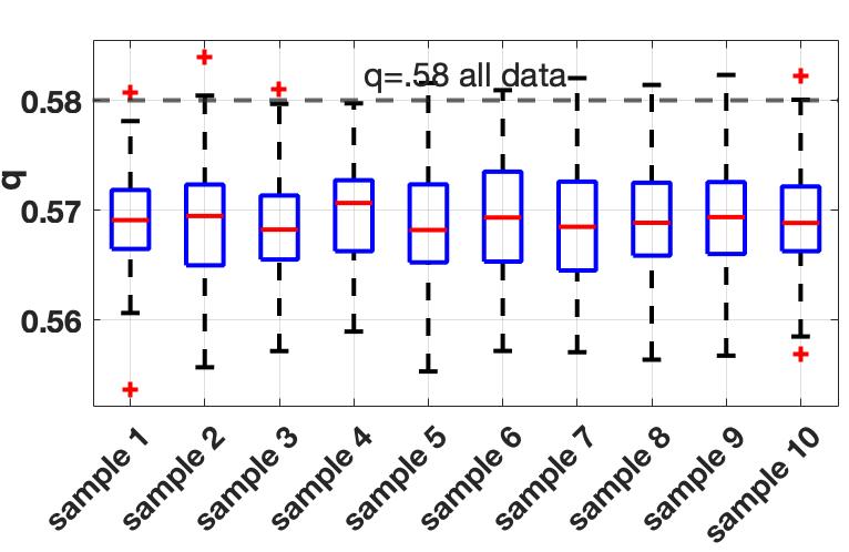
(a) Probability of Indicating Abandonment ($q$)

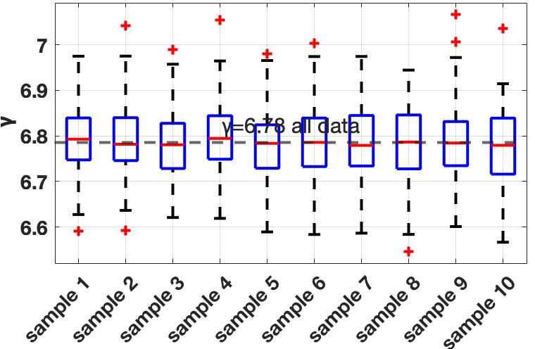
(b) Virtual Wait Time Parameter ($\gamma$)

Figure 12: Estimated $q$ and $\gamma$ Using the EM Algorithm in Samples of the Messaging Data

9.4 Accuracy of Estimations Using the Queueing Model

The accuracy analysis presented in in Sections 4.2.1 and 4.2.2 of the main paper assumed that customer patience and virtual wait time are independent and exponentially distributed, just like the EM algorithm assumption. However, the queueing model developed in Section 5 assumed a more realistic setting in which the data may incorporate some dependencies arising from the system dynamics. Specifically, the queueing simulation does not impose the exponential assumption on the virtual wait time; instead this variable is determined by the waiting and serving dynamics of the queueing system itself. Using this model we can test the robustness of the EM algorithm to the assumptions we made in Assumption 4.1. To do so, we check here the EM performance using simulated data obtained by that queueing model in two settings: (a) with the parameters of Yefenof et al. (2018) (§9.5) and (b) with the parameters of our messaging dataset (§9.6).

9.5 Queueing Simulation with the Parameters of Yefenof et al. (2018)

First we place ourselves in the setting found in Yefenof et al. (2018), where the parameters used in the simulation are $\theta=4$ and $q=0.5$. Since the queueing simulation does not impose a specific virtual wait time (i.e, a specific $\gamma$), we need to set this variable using the queueing dynamics. To do so, we calibrate $\mu$ so that the virtual wait time parameter is $\gamma=10$ (as in Yefenof et al. 2018). Figure 13(a) shows the accuracy of estimating $\theta$ using the five methods we compared in Section 4.2.1. The results are consistent with our previous results, suggesting that only the EM algorithm is able to estimate $\theta$ accurately. Figures 13(b) and 13(c) show the accuracy of estimating $q$ and $\gamma$, respectively. It can be seen that the EM estimates accurately $q$, whereas for $\gamma$ estimates it as accurately as most of the other methods.

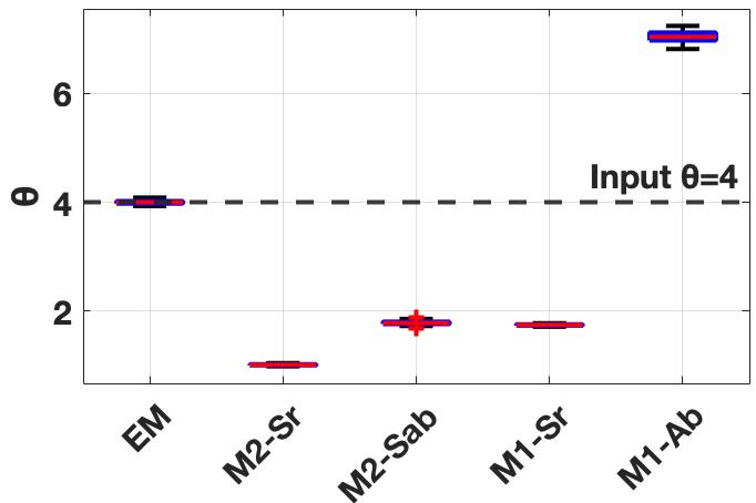
(a) Patience Parameter ($\theta$)

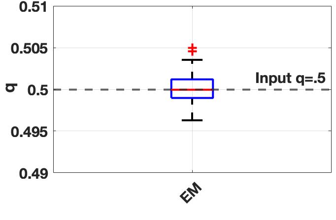
(b) Probability of Indicating Abandonment ($q$)

(c) Virtual Wait Time Parameter ($\gamma$)

Figure 13: Queueing Model Simulation ($\theta=4,q=0.5$, $\gamma=10$ as Determined by System Dynamics)

9.6 Queueing Simulation with the Parameters of the Messaging Dataset

In this simulation we used parameters that were evaluated from the real messaging data at a highly loaded time of the day (weekdays at 12:00). Specifically, the arrival rate is $\lambda=753$ customers per hour and the service rate is $\mu_{Regular}=1.22$; the service rate is calculated using the net time a conversation stayed open in the system (from agent assignment until the last message written by either the customer or the agent). For simplicity, we first assume that $\mu_{Sr}=\mu_{Sab}$. The number of full-time equivalent “agents” is $n=452$; it is taken to be the average number of online agents ($113$) per hour (either idling or serving customers) times 4, a typical average concurrency level in the system. Thus, $n$ represents the number of slots available for service and $q$ is taken to be 0.332, a result that follows from the following calculation:

$$q=\frac{Pr\left\{C_{2}=1\right\}}{Pr\{C_{2}=1\}+Pr\{C_{3}=1\}}=\frac{Pr\left\{C_{2}=1\right\}}{Pr\left\{C_{3}=1\mid M=0\right\}Pr\left\{M=0\right\}+Pr\left\{C_{2}=1\right\}},$$ (10)

where $Pr\left\{C_{2}=1\right\}=0.0716$ and $Pr\left\{M=0\right\}=0.2616$ are calculated using data on conversations without uncertainty (with complete data). $Pr\left\{C_{3}=1\mid M=0\right\}=0.55$ is obtained from the classification model of Section 3.2. The patience parameter $\theta$ is 0.739 hours; this is the result we obtained from the estimation of the EM algorithm in Section 4.2.3. We simulate our queueing model for a period of 1 month (with 100 repetitions), excluding a warm-up period of 2 hours till the system achieves steady state.

We estimate $\theta$, $q$, and $\gamma$ from the simulated data, using the EM algorithm, as well as the methods described in the main text (Mandelbaum and Zeltyn 2013, Yefenof et al. 2018). The results are presented in Figure 14(a). Again, the EM algorithm is the only method that is able to estimate accurately the customer patience rate, $\theta$, and it has no close competitor. The closest estimator to the EM is Yefenof et al. (2018) with $M=0$ considered as silent abandonment. However, note that this model estimates the average customer patience rate to be $\hat{\theta}=0.113$, implying that the average customer patience is $E[Patience]=\frac{60}{\hat{\theta}}=\frac{60}{0.113}=531.45$ minutes. We find this number to be unrealistic since to claim that a customer may be willing to wait almost 9 hours to be served is not reasonable; moreover, it is very far from the real average customer patience that we input into the simulation, which is 81.81 minutes. Accuracy results for the estimation of $q$ and $\gamma$ in this simulation are presented in Figures 14(b) and 14(c), respectively.

(a) Patience Parameter ($\theta$)

(b) Probability of Indicating Abandonment ($q$)

(c) Virtual Wait Time Parameter ($\gamma$)

Figure 14: Queueing Model Simulation, with Messaging System Parameters

10 Performance Measures Chat System Dataset

Table 7: Performance Measures Chat System Dataset (February 2017)

Performance Measure	Avg.	SD
$P\{\text{Wait}>0\}$	0.59	0.03
$P\{\text{Ab}\}$	0.23	0.04
E[Queue]	1.72	0.46
E[Wait]	2.41	0.72
E[Wait$|$Served]	2.04	0.58

References

- Aksin et al. (2013) Aksin Z, Ata B, Emadi SM, Su CL (2013) Structural estimation of callers’ delay sensitivity in call centers. Management Science .
- Aksin et al. (2017) Aksin Z, Ata B, Emadi SM, Su CL (2017) Impact of delay announcements in call centers: An empirical approach. Operations Research .
- Altman et al. (2019) Altman D, Ashtar S, Olivares M, Yom-Tov GB (2019) Do customer emotions affect worker speed? An empirical study of emotional load in online customer contact centers, Technion Working Paper.
- Armony et al. (2009) Armony M, Shimkin N, Whitt W (2009) The impact of delay announcements in many-server queues with abandonment. Operations Research 57(1):66–81.
- Baker et al. (1991) Baker DW, Stevens CD, Brook RH (1991) Patients who leave a public hospital emergency department without being seen by a physician: Causes and consequences. JAMA: The Journal of the American Medical Association 266(8):1085–1090.
- Batt and Terwiesch (2015) Batt RJ, Terwiesch C (2015) Waiting patiently: An empirical study of queue abandonment in an emergency department. Management Science 61(1):39–59.
- Brown et al. (2005) Brown L, Gans N, Mandelbaum A, Sakov A, Shen H, Zeltyn S, Zhao L (2005) Statistical analysis of a telephone call center: A queueing-science perspective. Journal of the American Statistical Association 100(469):36–50.
- Carmeli et al. (2019) Carmeli N, Mandelbaum A, Caspi H (2019) Modeling and analyzing voice-response systems, as a special case of self-services, Technion Working Paper.
- Fawcett (2006) Fawcett T (2006) An introduction to ROC analysis. Pattern Recognition Letters 27(8):861–874.
- Folkins et al. (1980) Folkins C, Hersch P, Dahlen D (1980) Waiting time and no-show rate in a community mental health center. American Journal of Community Psychology 8(1):121–123.
- Froehle and Roth (2004) Froehle CM, Roth AV (2004) New measurement scales for evaluating perceptions of the technology-mediated customer service experience. Journal of Operations Management 22(1):1–21.
- Galucci et al. (2005) Galucci G, Swartz W, Hackerman F (2005) Impact of the wait for an initial appointment on the rate of kept appointments at a mental health center. Psychiatric Services 56(3):344–346.
- Gans et al. (2003) Gans N, Koole G, Mandelbaum A (2003) Telephone call centers: Tutorial, review, and research prospects. Manufacturing and Service Operations Management 5(2):79–141.
- Garnett et al. (2002) Garnett O, Mandelbaum A, Reiman M (2002) Designing a call center with impatient customers. Manufacturing and Service Operations Management 4(3):208–227.
- Geraghty et al. (2008) Geraghty M, Glynn F, Amin M, Kinsella J (2008) Patient mobile telephone “text” reminder: A novel way to reduce non-attendance at the ENT out-patient clinic. Journal of Laryngology and Otology 122(3):296–298.
- Goes et al. (2018) Goes PB, Ilk N, Lin M, Zhao JL (2018) When more is less: Field evidence on unintended consequences of multitasking. Management Science 64(7):2973–3468.
- Ho and Lau (1992) Ho CJ, Lau HS (1992) Minimizing total cost in scheduling outpatient appointments. Management Science 38(12):1750–1764.
- Hosmer and Lemeshow (2002) Hosmer DW, Lemeshow S (2002) Applied Logistic Regression (John Wiley and Sons).
- Ibrahim and Whitt (2009) Ibrahim R, Whitt W (2009) Real-time delay estimation in overloaded multiserver queues with abandonments. Management Science .
- Kingman (1962) Kingman JFC (1962) On queues in heavy traffic. Journal of the Royal Statistical Society: Series B (Methodological) 24(2):383–392.
- Koole and Mandelbaum (2002) Koole G, Mandelbaum A (2002) Queueing models of call centers: An introduction. Annals of Operations Research 113(1):41–59.
- Larson (1990) Larson RC (1990) The queue inference engine: Deducing queue statistics from transactional data. Management Science 36(5):586–601.
- Little and Rubin (2002) Little R, Rubin D (2002) Statistical Analysis with Missing Data. Probability and Mathematical Statistics (Wiley).
- Liu (2016) Liu N (2016) Optimal choice for appointment scheduling window under patient no-show behavior. Production and Operations Management 25:128–142.
- Liu et al. (2010) Liu N, Ziya S, Kulkarni VG (2010) Dynamic scheduling of outpatient appointments under patient no-shows and cancellations. Manufacturing and Service Operations Management 12(2):189–370.
- Long et al. (2018) Long Z, Tezcan T, Zhang J (2018) Customer service chat systems with general service and patience times, Working Paper.
- Luo and Zhang (2013) Luo J, Zhang J (2013) Staffing and control of instant messaging contact centers. Operations Research 61(2):328–343.
- Mandelbaum and Zeltyn (2007) Mandelbaum A, Zeltyn S (2007) Service engineering in action: The Palm/Erlang-A queue, with applications to call centers. Spath D, Fähnrich KP, eds., Advances in Services Innovations, 17–45 (Springer).
- Mandelbaum and Zeltyn (2013) Mandelbaum A, Zeltyn S (2013) Data stories about (im)patient customers in tele-queues. Queueing Systems 75(2–4):115–146.
- Massad et al. (2006) Massad N, Heckman R, Crowston K (2006) Customer satisfaction with electronic service encounters. International Journal of Electronic Commerce 10(4):73–104.
- Medicare (2018) Medicare (2018) The official u.s. government site for medicare, hospital compare. Press Release, URL https://www.medicare.gov/hospitalcompare/, accessed: 2019-08-12.
- Moore et al. (2001) Moore CG, Wilson-Witherspoon P, Probst JC (2001) Time and money: Effects of no-shows at a family practice residency clinic. Family Medicine 33(7):522–527.
- Palm (1957) Palm R (1957) Research on Telephone Traffic Carried by Full Availability Groups (Tele).
- Rafaeli et al. (2017) Rafaeli A, Altman D, Gremler DD, Huang MH, Grewal D, Iyer B, Parasuraman A, de Ruyter K (2017) The future of frontline research: Invited commentaries. Journal of Service Research 20(1):91–99.
- RingCentral (2012) RingCentral (2012) Texting for work on the rise per ringcentral survey. Press Release, URL https://www.ringcentral.com/whyringcentral/company/pressreleases/pressreleases-2012/131212.html.
- Schumann et al. (2012) Schumann JH, Wünderlich NV, Wangenheim F (2012) Technology mediation in service delivery: A new typology and an agenda for managers and academics. Technovation 32(2):133–143.
- Smith (2002) Smith PJ (2002) Analysis of Failure and Survival Data (CRC Press).
- Tezcan and Zhang (2014) Tezcan T, Zhang J (2014) Routing and staffing in customer service chat systems with impatient customers. Operations Research 62(4):943–956.
- van Dolen and de Ruyter (2002) van Dolen WM, de Ruyter K (2002) Moderated group chat: An empirical assessment of a new e-service encounter. International Journal of Service Industry Management 13(5):496–511.
- Vissers (1979) Vissers J (1979) Selecting a suitable appointment system in an outpatient setting. Medical Care 17(12):1207–1220.
- Westphal (2018) Westphal M (2018) An experimental study of customer patience and abandonment in online customer service. Master’s thesis, Technion—Israel Institute of Technology.
- Whitt (2006) Whitt W (2006) Fluid models for multiserver queues with abandonments. Operations Research 54(1):37–54.
- Yefenof et al. (2018) Yefenof J, Goldberg Y, Wiler J, Mandelbaum A, Ritov Y (2018) Self-reporting and screening: Data with current-status and censored observations, Working Paper.