IDLL: Inverse Depth Line based Visual Localization in Challenging Environments

Abstract

Precise and real-time localization of unmanned aerial vehicles (UAVs) or robots in GNSS denied indoor environments are critically important for various logistics and surveillance applications. Vision-based simultaneously locating and mapping (VSLAM) are key solutions but suffer location drifts in texture-less, man-made indoor environments. Line features are rich in man-made environments which can be exploited to improve the localization robustness, but existing point-line based VSLAM methods still lack accuracy and efficiency for the representation of lines introducing unnecessary degrees of freedoms. In this paper, we propose Inverse Depth Line Localization (IDLL), which models each extracted line feature using two inverse depth variables exploiting the fact that the projected pixel coordinates on the image plane are rather accurate, which partially restrict the lines. This freedom-reduced representation of lines enables easier line determination and faster convergence of bundle adjustment in each step, therefore achieves more accurate and more efficient frame-to-frame registration and frame-to-map registration using both point and line visual features. We redesign the whole front-end and back-end modules of VSLAM using this line model. IDLL is extensively evaluated in multiple perceptually-challenging datasets. The results show it is more accurate, robust, and needs lower computational overhead than the current state-of-the-art of feature-based VSLAM methods.

I Introduction

Precisely positioning in large, challenging indoor environments is a key problem for robots, autonomous car parking, and mobile phone locating applications. Global navigation satellite systems (GNSSs) [1] cannot cover indoor areas where satellite signals are blocked [2]. Lidar-based methods require lidar devices and even multi-line lidar devices which generally have small view angle because indoor walls are very close, and have reflection problem for objects with glass surfaces[3]. As a result, vision-based methods, especially the visual–inertial fusion based localization systems, have drawn widespread attentions for accurate location and environment perception[4] in indoor environments. Moreover, the mono-cameras and inertial measurement units (IMUs) are both light-weight and low-cost, and as such they are the most widely used in civilian indoor localization applications.

However, recent works on visual–inertial odometry (VIO) have revealed the challenges of VIO in low-texture, low-light and fast movement scenarios. In the corridors, or parking lots etc., where the environments are structural similar and low-texture, the VIO system suffers drifting problem and provides unsatisfactory localization performances. Recent work solve localization problems in these scenarios by pursuing more contextual features from the environment.

One way is the semantic-based visual SLAM[5][6], which however needs much higher computation cost to detect and to track the visual objects. Therefore, another important approach for both accuracy and efficiency is to extract and utilize the line features [7, 8], because there are rich line features in the man-made indoor environments. However, the utilizing of the line features also introduce a large number of variables to determine the lines, since the directions and locations of lines need to be jointly determined with the ego-motions of the camera. For pursuing accurate and real-time state estimation, how to effectively utilize the line features is still a key problem. In this work, we represent each line via inverse depth line model and present several algorithmic innovations. This reduces the representation complexity of each line and makes the real-time localization in challenging environments feasible while also demonstrates superiority in terms of accuracy and efficiency when comparing to the state-of-the-arts of existing point-line based VIO methods.

More specifically, current VIO algorithms estimate a vehicle’s ego-motion in two stages: the front-end and the back-end. The front-end module is to pre-process the measurements from IMU and camera and the back-end module is to estimate the camera’s ego-motion trajectories and the states of point and line features. The front-end is generally classified into two categories, i.e., feature-based (indirect)[9, 10, 11] and direct methods[12]. Feature based methods show great success in widely used VIO systems, such as VIORB[10], ORB-SLAM3[11]. But in low-texture environments, the point based methods cannot extract a sufficient number of feature points. Line features are rich in these man-made environments. Previous work used OpenCV’s Line Segment Detector (LSD) algorithm[13] to detect line features. We observe that a large number of short line features are usually detected by LSD. However, they are difficult to match and may disappear in the next frame. As a result, computational resources to detect, describe, and match line features are wasted. Based on this observation, we focus on the main feature lines to improve the efficiency for feature line detection and matching. In the back-end optimization process, factor graph based optimization[14] methods demonstrate better accuracy than the extended Kalman filter (EKF) based methods[15]. This paper therefore focuses on the graph optimization based method.

After detection of the line features, the variables representing the features increase a large amount. This triggers the requirement of more observation functions to determine the variables and therefore makes the back-end optimization inefficient [7, 8]. The existing mainstream line representation is the orthonormal representation[7, 8, 16] with four parameters. But in fact, the projected line on the image plane is known in the line capturing instance, i.e., the normal vector formed by the spatial line and the camera origin is determined and its error is only related to the resolution of the image. So what we should optimize is the direction of the spatial line and its distance to the origin. We therefore propose to use the inverse depths of two endpoints to represent the spatial line, which need only two parameters. This dimension-reduced line representation is more robust and efficient. Also, because the inverse depths of the two endpoints are related to the camera pose, a two-step optimization method is proposed to speed up the optimization of the camera poses as well.

By integrating the aforementioned line extraction and representation with mono-camera based VIO method [14], an Inverse Depth Line based Localization method (IDLL) is proposed, whose key features include:

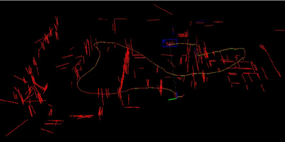
(a)

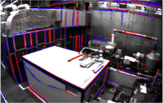
(b)

Figure 1: Trajectory and point-line feature map of IDLL on the MH-04-Difficult sequence. The two pictures are the screenshots of ROS Rviz window, where the green line denotes the motion trajectory, the red lines represent space tracked lines and the blue lines represent space non-tracked lines. (a) VIO trajectory and feature map window. (b) Feature tracked window.

• IDLL is a real-time optimization-based monocular VIO method using point and line features, which demonstrates accuracy and efficiency in challenging environments.

• A two-parameter representation for line based on endpoints’ inverse depth is presented. This dimensionally reduced line representation makes the line residual edges more robust and efficient in back-end optimization.

• Points, lines, and IMU information are fused efficiently in an optimization-based sliding window for high accuracy pose estimation.

• We present a two-step optimization method to further limit the computational complexity by introducing the long-term line association into the optimization process. Each step of optimization is easy to solve and we prove that this method can always converge.

• Experiments on the benchmark dataset EuRoc[17] show our method yields much higher localization accuracy in various challenging cases than state-of-the-arts methods.

II Related Work

Monocular vo and vslam algorithms have been studied for decade years, and achieved a lot. Such as direct method: DSO[18], LSD-SLAM[19], SVO[20], DPLVO[21] and EDPLVO[22] etc; featured-based method: PTAM[23], ORB-SLAM[24], PL-SLAM[25] etc. Although the monocular visual method has achieved good results, the monocular-based systems need a more complex system’s initialization, and the estimation of depth and scale often has some problems. For fix the monocular vision’s deficiency, other categories of cameras are used, such as RGBD, stereo[26]. Another way is multi sensor fusion, using monocular and IMU(inertial measurement unit) together is the common way which is our work method. Thus, we don’t introduce the other fusion methods of sensors too much. Adding an IMU may increase the information richness of the environment and make odometer estimation more accurate.

VI-SLAM or VIO algorithms can be divided in two stages: the front end and the back end. Table I provides a comparison of recent representative monocular VIO methods. The front end methods are generally classified into two categories, i.e., feature-based (indirect)[9, 10, 11] and direct methods[12].

TABLE I: Comparison of recent representative monocular VIO methods

Methods	Visual Feature		Framework		Coupled Mode		Loop Closure
	Point	Point+Line	Filter	Optimation	Loosely	Tightly
MSCKF[27]	✓		✓			✓
SR-ISWF[28, 29]	✓		✓			✓
ROVIO[30]	✓		✓			✓
OpenVINS[15]	✓		✓			✓	✓
VINS-Mono[14]	✓			✓		✓	✓
VIORB[10]	✓			✓		✓	✓
PL-VIO[7]		✓		✓		✓
PL-VINS[16]		✓		✓		✓	✓

The direct method uses the assumption of photometric invariance to estimate the camera motion by optimizing to minimize the photometric error at two corresponding locations in the image[31][30][12]. The direct method saves a lot of time in feature extraction and matching, and is easy to be ported to embedded systems and fused with IMUs. However, the photometric invariance is a strong assumption, which leads to the fact that the movement cannot be too fast or the illumination cannot change too much. Also if the gradient of the image alone is used to find the locus pose, it is easy to fall into local optimum due to the non-convexity of the image. We want to apply the real-time SLAM system in challenging indoor scenes, which require insensitivity to changes in ambient light and can meet the requirements of fast movement. Therefore, the feature-based methods are chosen to solve the visual localization problem in challenging indoor scenes.

The feature-based method estimates the camera pose by matching feature points to obtain the pose transformation[10][11][16][7][32]. The pose is further optimized by a nonlinear optimization method or extended Kalman filter (EKF) by landmarks (feature points). In the presence of loopback detection, the bag of words model [33] of feature points can be used to determine whether the robot detects loopback or not. The feature-based algorithm is less susceptible to the effects of illumination and movement speed because there are descriptors that are stable and robust to the visual features. Also, the bag of words model created by feature points can be used for loopback detection determination to correct errors. However, this method has difficulty in matching feature points for non-textured or weak textures, such as within tubular cavities, white walls, and indoor parking lots. Also the key points and descriptors consume more computational resources and the real-time performance is not as good as the direct methods.

Point-based methods: Most of existing methods exploit point-based features. OKVIS[9] extracted point features by using customized multi-scale SSE-optimized Harris corner detector[34]. It has good rotation invariance, scale invariance and robustness. BRISK algorithm[34] performs well in the registration of images with large blurring. VINS-Mono[14] is a monocular VIO benchmark as it produces highly competitive localization accuracy. It extracts point features by using Shi-Tomasi[35]. This algorithm is faster and more accurate than Harris corner detector[36]. Thus these works[31, 37, 38] use Shi-Tomasi to extract point features. The ORB-SLAM series [24][26][11], VIORB[10] mainly use ORB feature[39] which combines a FAST key-point detector[40] and a BRIEF descriptor[41]. ORB have good invariance to viewpoint. This allows to match them from wide baselines, boosting the accuracy of BA. And it a fast and lightweight alternative to SIFT. Now, neural networks are also used to extract point features[5]. But in challenging, textureless scenes reliable point features are hard to detect and track.

Point and line-based methods: Line features are also exploited in literature. PL-VIO[7] is the first optimization-based monocular VIO system using both points and lines as the landmarks. PL-VINS[16], another real-time and high-efficiency optimization-based monocular VINS method with point and line features, is developed based on VINS-Mono[14]. PL-VIO and PL-VINS both use KLT optical flow algorithm[42] to track point features. If the number of tracked point features is less than a threshold, new corner features will be detected by the FAST detector[40]. For line features, PL-VIO detected line segments by the LSD detector[13] in new frame, and matched with those in the previous frame by LBD descriptor[43]. This thread is slow, so PL-VIO does not support real-time. For efficiency of line detection, PL-VINS introduces a hidden parameter tuning and length rejection strategy to improve the performance of LSD algorithm. The modified LSD algorithm runs at least three times faster than the original LSD algorithm[13]. PL-VIO and PL-VINS perform frame-to-frame line feature matching between all the last and the current frame. Lines are represented by Plücker form [44] which consists of six parameters, line direction vector and the normal vector of the plane in line feature initialization step. PL-VIO and PL-VINS use orthonormal representation in optimization step because the Plücker coordinates are over-parameterized . It represents a line by four DoF (Degrees of Freedom) parameters, and has a superior performance in terms of convergence. When optimizing, PL-VIO only use feature constraints in reprojection error, but PL-VINS used the loop closure thread to correct drift error. PL-VIO and PL-VINS achieved good results in general cases. But the representation of lines in them uses redundant parameters. The accuracy and efficiency of point-line based method is further improved in this paper.

The backend module can be divided into two categories: filter-based methods[27, 28, 29] and optimization-based methods.

Filter-based methods: usually process a measurement only once in the updating step and based on EKF. A famous EKF based VIO approach is MSCKF[27]. MSCKF adds camera pose (position and pose quaternion) at different times to the state vector. The feature points seen by multiple cameras form geometric constraints between multiple camera states. SR-ISWF[28, 29] is an extension of MSCKF, which uses square root form to achieve single precision representation and avoids cross numerical characteristics. ROVIO[30] tracks multilevel patch features within the EKF, and introduces intensity errors as an innovation terms during the update step. Recently OpenVINS[15] is developed, an open platform, for visual-inertial estimation research for both the academic community and practitioners from industry. Some new works[8, 32, 45] introduce line features or plane features to improve localization accuracy of OpenVINS.

Optimization-based methods: Optimization-based methods minimize a joint nonlinear cost function with IMU measurement residuals and visual re-projection residuals to get the optimal result. Thus, optimization-based approaches can generally achieve better accuracy than the filtering-based methods. Previous methods mainly use point features to calculate the re-projection error [9, 14, 31, 37, 38, 10] and have achieved good results. However, in textureless environments and illumination-changing scenes, point features become unreliable. Poor feature tracking will lead to localization failure. More visual information needs to be introduced into the optimization method. Line segments are a proper alternative in challenging environments. Besides, line segments provide more structural information in the challenging environments than points. So, more work began to introduce line feature into the optimization-based method[7][16].

Nowadays, deep learning techniques outperform traditional methods in various computer vision tasks. In terms of VIO, learning-based approaches have made significant progress in recent years. However, these methods generally require a powerful GPU. Readers may refer to the recent surveys [46][47] for deep learning based VIO methods.

Overall, seeing the remaining challenges of visual localization in challenging environments, this paper presents IDLL, a real-time optimization-based monocular visual-inertial SLAM method with point and line features, in which we exploit the inverse depth representation of lines to improve the accuracy, robustness and efficiency of visual inertial localization.

III Problem Model and Inverse Depth Line Geometry

We consider an autonomous agent, such as a UAV, a UGV, or a robot is moving in an GNSS denied indoor environment. The agent is equipped with a monocular camera and an embedded IMU, which takes images in frequency $f_{c}$ and takes accelerator and gyroscope readings in frequency $f_{i}$ for estimating the agent’s ego-motion and the surrounding environments simultaneously.

Before introducing the structure, we define three necessary coordinate frames: world frame ${\pi_{w}}$, IMU body frame ${\pi_{b}}$, and camera frame ${\pi_{c}}$. The gravity direction is aligned with the $z$-axis of ${\pi_{w}}$.

For each incoming image captured by the camera, point and line features are detected and tracked. For the point features, we use Shi-Tomasi[35] to detect, KLT[42] to track, and RANSAC-based epipolar geometry constraint[48] to identify inliers. As to the line features, line segments in new frame are detected by the LSD detector[13] and described by LBD descriptor[43]. We match the line segments with LBD descriptors in two consecutive frames by KNN[49] to track them and use geometric constraints to remove outliers of line matches. We use $\{c_{1},c_{2},\cdots,\}$ to represent the camera poses at different time instances. $F^{i}_{c_{1}}$ and $L^{i}_{c_{1}}$ are used to represent the $i$th point feature and the $i$th line feature captured by a camera at $c_{1}$ respectively. The superscript will be omitted if we refer to a specific point or a line. The transformation from the world frame to the camera frame at $c_{1}$ is denoted by $\mathbf{T}_{wc_{1}}=\left(\begin{matrix}\mathbf{R}_{wc_{1}}&\mathbf{t}_{wc_{1}}\\ \mathbf{0}^{T}&1\\ \end{matrix}\right)$. For the IMU, we pre-integrate new IMU measurements [50] between two consecutive frames to update the newest body states. We then introduce the different representation of the line features.

III-A Line Feature Representation

Traditionally, a line in 3D space is widely represented by six parameter Plücker coordinates[44]. In 2015, Zhang et al. [51] proposed four parameter orthonormal representation for 3D line, for the purpose of state optimization. They show the four parameter model for a 3-D line shows a superior performance in terms of accuracy and convergence in iterative line state optimization.

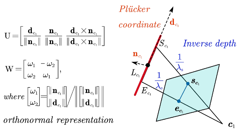
Figure 2: Different representation of a line.

III-A1 Plücker Coordinate Representation

We consider a 3-D line is captured at two camera poses $c_{1}$ and $c_{2}$ as shown in Fig. 2. We firstly consider the line representation for ${L_{{c_{1}}}}\in{\pi_{{c_{1}}}}$ in the first camera frame. The Plücker coordinates describe the line with ${L_{{c_{1}}}}=(\mathbf{n}_{{}_{{c_{1}}}}^{\top},\mathbf{d}_{{}_{{c_{1}}}}^{\top})^{\top}\in{\mathbb{R}^{6}}$, where $\mathbf{n}_{{c_{1}}}\in{\mathbb{R}^{3}}$ denotes the normal vector of the plane determined by $L_{{c_{1}}}$ and the origin of ${\pi_{{c_{1}}}}$. $\mathbf{d}_{{c_{1}}}\in{\mathbb{R}^{3}}$ denotes the direction vector determined by the two endpoints of ${L_{{c_{1}}}}$. The Plücker coordinates are over-parameterized with a constraint $\mathbf{n}_{{}_{{c_{1}}}}^{\top}\mathbf{d}_{{}_{{c_{1}}}}=0$, so their dimension can be further reduced.

III-A2 Orthonormal Representation

Zhang et al. verified that the Plücker coordinates can be described with a minimal four-parameter orthonormal representation[51]. In the orthonormal representation, $(\mathrm{U},\mathrm{W})\in SO(3)\times SO(2)$ can be calculated from ${L_{{c_{1}}}}=(\mathbf{n}_{{}_{{c_{1}}}}^{\top},\mathbf{d}_{{}_{{c_{1}}}}^{\top})^{\top}$ as:

$$\mathrm{U}=\left[\frac{\mathbf{d}_{c_{1}}}{\left\|\mathbf{n}_{c_{1}}\right\|}\,\,\frac{\mathbf{n}_{c_{1}}}{\left\|\mathbf{n}_{c_{1}}\right\|}\,\,\frac{\mathbf{d}_{c_{1}}\times\mathbf{n}_{c_{1}}}{\left\|\mathbf{d}_{c_{1}}\times\mathbf{n}_{c_{1}}\right\|}\right]$$ (1)

$$\mathrm{W}=\left[\begin{matrix}\omega_{1}&\!\!-\omega_{2}\\ \omega_{2}&\!\!\omega_{1}\\ \end{matrix}\right],\!where\!\,\,\left[\!\!\begin{array}[]{c}\omega_{1}\\ \omega_{2}\\ \end{array}\!\!\right]\!\!=\!\!{{\left[\!\!\begin{array}[]{c}\left\|\mathbf{n}_{c_{1}}\right\|\\ \left\|\mathbf{d}_{c_{1}}\right\|\\ \end{array}\!\!\right]}\Bigg{/}{\left\|\left[\!\!\begin{array}[]{c}\left\|\mathbf{n}_{c_{1}}\right\|\\ \left\|\mathbf{d}_{c_{1}}\right\|\\ \end{array}\!\!\right]\right\|}}$$ (2)

In practice, $\mathrm{U},\mathrm{W}$ can be computed using the QR decomposition of $\left[\begin{matrix}\mathbf{n}_{c_{1}}&\mathbf{d}_{c_{1}}\\ \end{matrix}\right]$:

$$\left[\begin{matrix}\mathbf{n}_{c_{1}}&\mathbf{d}_{c_{1}}\\ \end{matrix}\right]=\mathrm{U}\left[{\begin{array}[]{*{20}{l}}{{\omega_{1}}}&0\\ 0&{{\omega_{2}}}\\ 0&0\end{array}}\right],and~{}\mathrm{W}=\left[{\begin{array}[]{*{20}{c}}{{\omega_{1}}}&{{\omega_{2}}}\\ {-{\omega_{2}}}&{{\omega_{1}}}\end{array}}\right]$$ (3)

where $\mathrm{U}$ and $\mathrm{W}$ denote a three and a two dimensional rotation matrix $R(\bm{\theta})$ and $R(\theta)$ respectively. So the line is essentially represented by four parameters $\mathbf{p}^{\top}=(\bm{\theta}^{\top},\theta)$. Converting from the orthonormal representation to Plücker coordinates is easy, which is:

$$\left[\begin{matrix}\mathbf{n}_{c_{1}}&\mathbf{d}_{c_{1}}\\ \end{matrix}\right]=\left[\omega_{1}\mathbf{u}_{1}^{\top},\omega_{2}\mathbf{u}_{2}^{\top}\right]$$ (4)

where $\mathbf{u}_{i}$ is the $i$th column of $\mathrm{U}$.

Although the orthonormal representation of line reduces dimension and can speed up convergence, both it and the Plücker coordinates haven’t considered the context provided by the projected line in the captured image.

III-A3 Inverse Depth Representation

Because two points determine a straight line, we exploit the inverse depth representation of two end points to further reduce the parameter dimension of a 3-D line. Considering the 3-D line $L_{c_{1}}$ when it is captured by the camera $c_{1}$ as shown in Fig.2. Suppose two points on the line under the camera $c_{1}$’s coordinate system are $S_{c_{1}}=(x_{s}^{{c_{1}}},y_{s}^{{c_{1}}},z_{s}^{{c_{1}}})$ and $E_{c_{1}}=(x_{e}^{{c_{1}}},y_{e}^{{c_{1}}},z_{e}^{{c_{1}}})$. They are represented in the normalized camera coordinate system as $s_{c_{1}}=(u_{s}^{{c_{1}}},v_{s}^{{c_{1}}},1)$ and $e_{c_{1}}=(u_{e}^{{c_{1}}},v_{e}^{{c_{1}}},1)$ as shown in Fig.2. In the same way as the space point, the following equation can be obtained.

$$\begin{gathered}S_{c_{1}}=(x_{s}^{{c_{1}}},y_{s}^{{c_{1}}},z_{s}^{{c_{1}}})=\frac{1}{{{\lambda_{s}}}}(u_{s}^{{c_{1}}},v_{s}^{{c_{1}}},1)=\frac{1}{{{\lambda_{s}}}}s_{c_{1}}\hfill\\ E_{c_{1}}=(x_{e}^{{c_{1}}},y_{e}^{{c_{1}}},z_{e}^{{c_{1}}})=\frac{1}{{{\lambda_{e}}}}(u_{e}^{{c_{1}}},v_{e}^{{c_{1}}},1)=\frac{1}{{{\lambda_{s}}}}e_{c_{1}}\hfill\\ \end{gathered}$$ (5)

where $\lambda_{s}$ and $\lambda_{e}$ are the inverse depth of the two endpoints. According to the geometric principle, the normal vector $\mathbf{n}_{{c_{1}}}$ is the cross product of the vectors formed by the origin and the two points, and the direction vector $\mathbf{d}_{{c_{1}}}$ is the vector obtained by subtracting the two points. Because the endpoints’ projected pixels on the image plane, i.e., $(u_{s}^{{c_{1}}},v_{s}^{{c_{1}}})$, $(u_{e}^{{c_{1}}},v_{e}^{{c_{1}}})$ are known, given two inverse depth parameters $l=(\lambda_{s},\lambda_{e})$, we can recover the Plücker coordinates by:

$$\begin{gathered}\mathbf{n}_{{c_{1}}}=\frac{1}{{{\lambda_{s}}}}(u_{s}^{{c_{1}}},v_{s}^{{c_{1}}},1)\times\frac{1}{{{\lambda_{e}}}}(u_{e}^{{c_{1}}},v_{e}^{{c_{1}}},1)\hfill\\ \mathbf{d}_{{c_{1}}}=\frac{1}{{{\lambda_{e}}}}(u_{e}^{{c_{1}}},v_{e}^{{c_{1}}},1)-\frac{1}{{{\lambda_{s}}}}(u_{s}^{{c_{1}}},v_{s}^{{c_{1}}},1)\hfill\\ \end{gathered}$$ (6)

In this way we have reduced the line representation from 6 degrees of freedom to 2 degrees of freedom, i.e., $\lambda_{s}$ and $\lambda_{e}$. Comparing with the orthonormal representation which uses 4 degrees of freedom to optimize, the inverse depth representation utilizes the knowledge that the endpoints’ projected coordinate $\{(u_{s},v_{s}),(u_{e},v_{e})\}$ on the camera plane are known and are rather accurate. The uncertainty of $u,v$ depends on the resolution of the image. So that the line is restricted in the plane formed by the projected line and the camera optical center. The two endpoints depth value $d_{s},d_{e}$, and so that the reverse depth parameters $\lambda_{s}=\frac{1}{d_{s}}$, $\lambda_{e}=\frac{1}{d_{e}}$ are the key parameters to determine the 3-D line in this scenario.

Given a detected line feature and its endpoints’ projected coordinates on the image, the 3-D line can then be determined by optimizing the two inverse depth scalar values. Since there are many line features can be detected in each frame, by reducing each line’s degree of freedom, the problem’s state dimension is greatly reduced, which provides better overall accuracy and efficiency to the point-line based VSLAM.

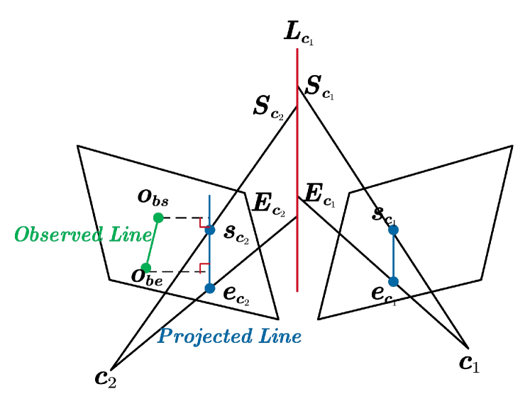
Figure 3: Line residual of a observed line in sliding window. The line reprojection residual is modeled in terms of point-to-line distance.

III-B Line’s Reprojection Residual Error Model

During the frame-to-frame simultaneously camera ego-motion and point-line coordinate determination, VSLAM sets up residual error minimization objective and uses graph optimization to solve the optimization problem [9]. The point-based reprojection residual error and the IMU’s pre-integration residual error have been thoroughly introduced in [14]. In this subsection, we only introduce the line feature’s reprojection residual error model using the inverse depth representation of lines.

The line reprojection residual is modeled in terms of point-to-line distance as shown in Fig.3. At first, we define line geometry transformation. Let ${\mathbf{R}_{w{c_{1}}}},{\mathbf{R}_{w{c_{2}}}}\in SO(3)$ and ${\mathbf{t}_{w{c_{1}}}},{\mathbf{t}_{w{c_{2}}}}\in\mathbb{R}^{3}$ be the rotation matrices and translation vectors from $\pi_{w}$ to $\pi_{c_{1}}$, and from $\pi_{w}$ to $\pi_{c_{2}}$ respectively. With these matrices, by knowing the line $L_{c_{1}}$ captured by $c_{1}$, represented by (6), we can transform $L_{c_{1}}$ in $\pi_{c_{1}}$ to $L_{c_{2}}$ in $\pi_{c_{2}}$ by the line transformation equation [44]:

$$\begin{gathered}L_{w}\!=\!\left[\!\begin{array}[]{c}\mathbf{n}_{w}\\ \mathbf{d}_{w}\\ \end{array}\!\right]\!=\!\mathbf{T}_{wc_{1}}L_{c_{1}}\!=\!\left[\!\begin{matrix}\mathbf{R}_{wc_{1}}\!\!&\!\!\left[\mathbf{t}_{wc_{1}}\right]_{\times}\mathbf{R}_{wc_{1}}\\ 0\!\!&\!\!\mathbf{R}_{wc_{1}}\\ \end{matrix}\!\right]\left[\!\begin{array}[]{c}\mathbf{n}_{c_{1}}\\ \mathbf{d}_{c_{1}}\\ \end{array}\!\right]\hfill\\ L_{c_{2}}=\left[\begin{array}[]{c}\mathbf{n}_{c_{2}}\\ \mathbf{d}_{c_{2}}\\ \end{array}\!\right]=\mathbf{T}_{c_{2}w}L_{w}={\mathbf{T}_{wc_{2}}}^{-1}L_{w}\hfill\\ =\left[\begin{matrix}\mathbf{R}_{wc_{2}}^{\top}\!\!&\!\!-{\mathbf{R}_{wc_{2}}}^{\top}\left[\mathbf{t}_{wc_{2}}\right]_{\times}\\ 0\!\!&\!\!{\mathbf{R}_{wc_{2}}}^{\top}\\ \end{matrix}\right]\left[\begin{matrix}\mathbf{R}_{wc_{1}}\!\!&\!\!\left[\mathbf{t}_{wc_{1}}\right]_{\times}\mathbf{R}_{wc_{1}}\\ 0\!\!&\!\!\mathbf{R}_{wc_{1}}\\ \end{matrix}\right]\left[\!\!\begin{array}[]{c}\mathbf{n}_{c_{1}}\\ \mathbf{d}_{c_{1}}\\ \end{array}\!\!\right]\hfill\\ \end{gathered}$$ (7)

Next, the estimated projection line $\mathbf{l}$ on $c_{2}$’s image frame is obtained by transforming $L_{c_{2}}$ to the image plane[51]:

$$\mathbf{l}=\left[l_{1},l_{2},l_{3}\right]^{\top}={\mathbf{K}_{L}}{\mathbf{n}_{{c_{2}}}}$$ (8)

where ${\mathbf{K}_{L}}=\left[{\begin{array}[]{*{20}{c}}{{f_{y}}}&0&0\\ 0&{{f_{x}}}&0\\ {-{f_{y}}{c_{x}}}&{-{f_{x}}{c_{y}}}&{{f_{x}}{f_{y}}}\end{array}}\right]$ denotes the line projection matrix and $\mathbf{n}_{c_{2}}$ can be extracted from (7). Note that $L_{c_{1}}=[\mathbf{n}_{c_{1}}^{\top},\mathbf{d}_{c_{i}}^{\top}]^{\top}$ is determined by the two inverse depth parameters in (6).

Finally, assume that $L^{i}_{c_{1}}$ corresponds to the $i$-th matched line feature which is simultaneously observed by $c_{1}$ and $c_{2}$, denoted by $\mathbf{l}_{i}$ on $c_{1}$ . Suppose the measured endpoints of this line on $c_{2}$ image plane is $s_{c_{2}}$ and $e_{c_{2}}$ respectively. Then this line’s re-projection error can be calculated by the point to line distance.

$$r_{l}(z_{\mathbf{l}_{i}}^{c_{1}},\mathcal{X})=\left[\begin{array}[]{c}d(s_{c_{2}},\mathbf{l})\\ d(e_{c_{2}},\mathbf{l})\\ \end{array}\right]=\left[\begin{array}[]{c}\frac{{s_{c_{2}}}^{\top}\mathbf{l}}{\sqrt{l_{1}^{2}+l_{2}^{2}}}\\ \frac{{e_{c_{2}}}^{\top}\mathbf{l}}{\sqrt{l_{1}^{2}+l_{2}^{2}}}\\ \end{array}\right]$$ (9)

where $d({s_{{c_{2}}}},\mathbf{l})$ and $d({e_{{c_{2}}}},\mathbf{l})$ denote the point-to-line distance function. $s_{{c_{2}}}$ and $e_{{c_{2}}}$ are the homogeneous coordinates of the endpoints of the line in $c_{2}$’s image frame. In calculating the residual error, an important property should be noted.

Although we use the inverse depth of the two endpoints to represent the line feature, we use the distance from the endpoint of the observation line to the line feature projection line to represent the reprojection error. This is because as the camera angle of view moves, line features will have problems such as endpoint repeatability, occlusion, or line segment deformation caused by the change of angle of view. In this way, the use of endpoint alignment is not accurate.

Theorem 1.

In calculating the frame-to-frame line re-projection residual error using the matched line segment captured by $c_{1}$ and $c_{2}$, denoted by $L_{c_{1}}$ and $L_{c_{2}}$, these two captured line segements don’t need to have common end vertices in the world frame.

Proof.

Suppose $L_{c_{1}}$ and $L_{c_{2}}$ are the captured line segments of $c_{1}$ and $c_{2}$ to a world frame line $L_{w}$. As can be seen from Fig.3, even if the observed endpoints $S_{c_{1}},E_{c_{1}}$’s world coordinates are different from the world coordinates of $S_{c_{2}},E_{c_{2}}$, the line re-projection error in (9) can be correctly calculated. This is because the residual error is calculated by the point-to-line distance instead of endpoint-to-endpoint distance. So $L_{c_{1}}$ and $L_{c_{2}}$ don’t need to observe the common endpoints of the line $L_{w}$. ∎

This property gives high flexibility in constructing the line re-projection residual errors using LSD-based line features, since the LSD detector provide two endpoints of the line in the image frame[13]. No matter whether the endpoints are from common points, only if they are from the same line, the residual error can be successfully constructed.

Knowing the residual error function, in graph optimization, we need to further calculate the corresponding Jacobian matrix $J$ for updating the line parameter $\lambda_{e}$ and $\lambda_{s}$. The derivation of the Jacobian matrix can be obtained by the chain rule, which is given in Appendix Appendix.

III-C Inverse Depth Line State Initialization

After setting the graph optimization model, the state variables needs to be initialized before conducting the iterative optimization. The camera poses can be initialized by IMU integration and the feature point locations can be initialized by triangulation method[14]. In this subsection, we mainly introduce how to initialize the two endpoints inverse depth $\lambda_{s},\lambda_{e}$ for each line segment.

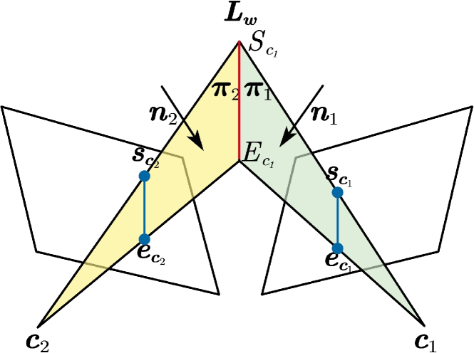
Figure 4: Initialization of a newly observed line. The straight line $L_{c_{1}}$ can be seen as the intersection of two planes $\pi_{1}$ and $\pi_{2}$ to obtain, that is, this line is in both planes and the distance to both planes is 0.

Consider the instance showing in Fig.4 when a line is captured by two camera frames. let’s assume that $L_{w}$ is observed by two camera poses, whose camera centers are $c_{1}$ and $c_{2}$ respectively. Then two planes are determined by the two camera positions and $L_{w}$, which are denoted $\pi_{1}=(c_{1},L_{w})$ and $\pi_{2}=(c_{2},L_{w})$. The line $L_{w}$ is the intersection of the two planes, so its distance to both planes is 0.

As shown in the Fig.4, the normal vector of the plane $\pi_{2}$ in $c_{2}$’s coordinate system can be represented by $\mathbf{n}_{2}=s_{c_{2}}\times e_{c_{2}}$, which is the cross product of the two vectors on the plane. Then the normal vector of the plane $\pi_{2}$ in $c_{1}$’s coordinate system can be represented by $\mathbf{n}_{2}^{c_{1}}=\mathbf{R}_{{c_{1}}{c_{2}}}s_{c_{2}}\times e_{c_{2}}$, where $\mathbf{R}_{{c_{1}}{c_{2}}}$ is the rotation matrix from $\pi_{c_{1}}$ to $\pi_{c_{2}}$. Then plane $\pi_{2}$ can be expressed in point-normal form as $\pi_{2}=\{{{\mathbf{n}_{2}}^{c_{1}}},-{{\mathbf{n}_{2}}^{c_{1}}}\cdot{c_{2}}\}$. We can then convert $\pi_{2}$’s representation to its general representation [52] which has four parameters $(\pi_{A}^{c_{2}},\pi_{B}^{c_{2}},\pi_{C}^{c_{2}},\pi_{D}^{c_{2}})$: where

$$\pi_{A}^{c_{2}},\pi_{B}^{c_{2}},\pi_{C}^{c_{2}}=\mathbf{n}_{2}^{c_{1}},\pi_{D}^{c_{2}}=-\mathbf{n}_{2}^{c_{1}}\cdot c_{2}$$ (10)

The observation of $L_{w}$ is $L_{c_{1}}$ in $c_{1}$’s coordinate frame. We then conduct following analysis in $c_{1}$’s coordinate frame. The two endpoints of $L_{c_{1}}$, i.e., $S_{c_{1}}$ and $E_{c_{1}}$ are on $L_{c_{1}}$, which is on plane $\pi_{2}$. So the distance from each endpoint to the plane $\pi_{2}$ is $0$. So we get the two endpoints’ inverse depth $\lambda_{s},\lambda_{e}$ from the following equation.

$$\begin{array}[]{c}d\left(S_{c_{1}},\pi_{2}\right)=\frac{|(\pi_{A}^{c_{2}},\pi_{B}^{c_{2}},\pi_{C}^{c_{2}})\cdot S_{c_{1}}+\pi_{D}^{c_{2}}|}{\sqrt{{\pi_{A}^{c_{2}}}^{2}+{\pi_{B}^{c_{2}}}^{2}+{\pi_{C}^{c_{2}}}^{2}}}=0\\ d\left(E_{c_{1}},\pi_{2}\right)=\frac{|(\pi_{A}^{c_{2}},\pi_{B}^{c_{2}},\pi_{C}^{c_{2}})\cdot E_{c_{1}}+\pi_{D}^{c_{2}}|}{\sqrt{{\pi_{A}^{c_{2}}}^{2}+{\pi_{B}^{c_{2}}}^{2}+{\pi_{C}^{c_{2}}}^{2}}}=0\\ \end{array}$$ (11)

where $d\left(S_{c_{1}},\pi_{2}\right)$ and $d\left(E_{c_{1}},\pi_{2}\right)$ are the distances from the two endpoints to the plane $\pi_{2}$. $S_{{c_{1}}}=\frac{1}{{{\lambda_{s}}}}(u_{s}^{{c_{1}}},v_{s}^{{c_{1}}},1)$ and $E_{{c_{1}}}=\frac{1}{{{\lambda_{e}}}}(u_{e}^{{c_{1}}},v_{e}^{{c_{1}}},1)$ are the spatial coordinates of the two endpoints. So (11) sets up two equations for two variables and the initial values of $\lambda_{s}$ and $\lambda_{e}$ can be calculated.

In reality, we often observe the same line in multiple frames, so we can get overdetermined equations(12).

$$\left[{\begin{array}[]{*{20}{c}}{\begin{array}[]{*{20}{c}}{d({S_{{c_{1}}}},{\pi_{2}})}\\ {d({E_{{c_{1}}}},{\pi_{2}})}\end{array}}\\ \vdots\\ {\begin{array}[]{*{20}{c}}{d({S_{{c_{1}}}},{\pi_{i}})}\\ {d({E_{{c_{1}}}},{\pi_{i}})}\end{array}}\end{array}}\right]=0$$ (12)

We can use the nonlinear least squares method [53] to optimize the solution $\lambda_{s},\lambda_{e}$ of the equations.

Remark: The initialization method in (11) avoid the effect caused by the inability to find the direction vector in the Plücker matrix method [48] when the transformation between $c_{1}$ and $c_{2}$ contains only rotation. The Plücker matrix method uses the following equation.

$$\left[{\begin{array}[]{*{20}{c}}{{{\left[{{\mathbf{d}_{{c_{1}}}}}\right]}_{\times}}}&{{\mathbf{n}_{{c_{1}}}}}\\ {-\mathbf{n}_{c_{1}}^{\top}}&0\end{array}}\right]={\pi_{1}}{\pi_{2}^{\top}}-{\pi_{2}}{\pi_{1}^{\top}}$$ (13)

where $\left[\cdot\right]_{\times}$ denotes the skew-symmetric matrix of a 3-vector. If the rotation-only case occurs, the wrong initialization value will be given to the arbitrary direction vector $\mathbf{d}_{{c_{1}}}$[48]. But for the inverse depth initialization in (12), in rotation-only case, the distances $d\left(S_{c_{1}},\pi_{i}\right)$ and $d\left(E_{c_{1}},\pi_{i}\right)$ in the iteration of the least squares method will always be 0, no residual edges will be introduced. Our method will not introduce wrong results, and the initialization result is better.

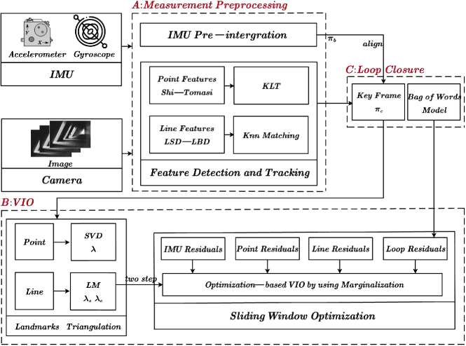
Figure 5: System overview of IDLL. It implements three threads including measurement preprocessing, VIO, and loop closure.

IV IDLL: Inverse Depth Line based Point-line VISLAM

Based on the inverse depth line representation, the residue error function, and the initialization method, we integrate the inverse depth line features in VISLAM and develop IDLL. This section will introduce the IDLL framework. The system architecture of IDLL is shown in Fig.5. IDLL contains three threads: (1) measurement processing, which conducts IMU pre-integration, point, and line feature extraction and matching; (2) the Vision Inertial Odometry (VIO) thread, which calculates the camera ego-motion and point-line locations by graph optimization in a sliding window; (3) the loop closure thread, which uses the bag-of-words model of points to conduct loop detection.

IV-A Measurement Processing

The first thread of IDLL extracts and aligns information from the raw measurements of the camera and IMU. For the image obtained from the camera, our algorithm will detect and track point and line features. For the point features, we use the method proposed by Shi-Tomasi[35] to detect, KLT[42] to track, and RANSAC-based epipolar geometry constraint[48] to identify inliers. As to the line features, line segments in the new frame are detected by the LSD detector[13] and described by LBD descriptor[43]. We match the line segments with LBD descriptors in two consecutive frames by KNN[49] to track them, and remove outliers of line matches geometric constraints. The sampling frequency of IMU is higher than the publishing frequency of image frames, so the IMU information between two adjacent image frames needs to be integrated to align with the visual information. We pre-integrate new IMU measurements between two consecutive frames to update the newest body states.

With these two types of preprocessed information, IDLL initializes some necessary parameters for triggering the visual-inertial odometry thread. First, it constructs a graph structure of poses, including the points and lines of the environment in the selected keyframes. The keyframes are selected to reduce the number of estimated states and the amount of optimization calculation. Here, we still use the VINS-Mono[14] keyframe selection method. There are two criteria for the selection of keyframes:

• The average parallax of the previous frame. If the average parallax of the tracking feature exceeds a certain threshold, we will choose it as a keyframe.

• The tracking quality. If the number of tracking features is less than a threshold, we will select this frame as a new keyframe.

Next, the graph is aligned with the pre-integrated IMU states using the initialization method in VINS-Mono[14]. The newest body states are used as the initial value in the sliding window optimization and the point-line triangulation.

IV-B Visual-Inertial Odometry

IDLL uses a two-step tightly-coupled optimization-based visual-inertial odometry (VIO) thread for high-accuracy pose estimation by minimizing all measurement residuals. VIO mainly consists of three parts: construction of sliding window, initialization of features, and optimization calculation of states. The specific process of VIO is as follows:

• First, judge whether the system is initialized. For monocular systems, the vision system can only obtain two-dimensional information and lose one-dimensional information (depth), so it needs to move, that is, triangulation to regain the lost depth information. However, the depth information recovered by triangulation is a ”pseudo depth”, and its scale is random and not real, so IMU is required to calibrate this scale. If you want the IMU to calibrate this scale, you need to move the IMU to get the state $p$ of $p,v,q$. We continue to use the SFM method[54] in VINS-Mono[14] for initialization calibration, which only be performed once.

• Then we use the sliding window algorithm to save the observation information and construct the residual edge of the state to be optimized. When a new frame comes, if the second new image frame in the sliding window is a key frame, the oldest frame and the above road marking point will be marginalized; If the second new image frame in the sliding window is not a key frame, the visual measurement information on this frame is discarded, and the IMU pre integration is transmitted to the next frame. Ensure that the key frame in the window always has a fixed value of 10 frames.

• After that, our system initializes the features, giving the initial value of the states to be optimized, and waiting for optimization.

• Finally, if the sliding window is full, optimize the states; otherwise, wait until the sliding window is full.

The detailed introduction of specific steps are in the followings:

IV-B1 Sliding Window Formulation

First, we adopt a fixed-size sliding window to find the optimal state vector, while achieving both computation efficiency and high accuracy, The full state variables in a sliding window at time $i$ are defined as:

$$\begin{gathered}\mathcal{X}=\left[{{\mathbf{x}_{0}},{\mathbf{x}_{1}},...,{\mathbf{x}_{n}},\mathbf{x}_{bc},{\lambda_{0}},{\lambda_{1}},...,{\lambda_{{n_{p}}}},{\mathbf{l}_{0}},{\mathbf{l}_{1}},...,{\mathbf{l}_{{n_{l}}}}}\right]\hfill\\ {\mathbf{x}_{k}}=\left[{{p_{wb_{k}}},{q_{wb_{k}}},{v_{wb_{k}}},{b_{a}},{b_{g}}}\right],k\in\left[{0,n}\right]\hfill\\ {\mathbf{x}_{bc}}=\left[{{p_{bc}},{q_{bc}}}\right]\hfill\\ {\mathbf{l}_{m}}=\left[{\lambda_{s_{m}},\lambda_{e_{m}}}\right],m\in\left[{0,{n_{l}}}\right]\hfill\\ \end{gathered}$$ (14)

where $\mathbf{x}_{k}$ contains the $k$-th IMU body position ${p_{wb_{k}}}$, orientation ${q_{wb_{k}}}$, velocity ${v_{wb_{k}}}$ in $\pi_{w}$, acceleration bias $b_{a}$, gyroscope bias $b_{g}$. $n$, $n_{p}$, and $n_{l}$ denote the total number of keyframes, space points and lines in the sliding window, respectively. $\lambda$ is the inverse distance of a point feature from its first observed keyframe. $\mathbf{l}$ is the inverse depth representation of a 3D line feature from its first observed keyframe.

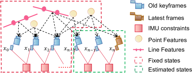
Figure 6: Factor graphs of visual–inertial SLAM with point and line landmarks.

Figure 7: A schematic of our algorithm for one 3D line and the sliding window of size three and Hessian matrix. For our two-step minimization algorithm, the Hessian matrix become smaller, iterations become faster.

For vision-inertial fusion, we use a factor-graph-based tightly-coupled framework to optimize all state variables as shown in Fig.6. The nodes are the IMU body states to be optimized or the 3D landmarks to be optimized. The edges represent the measurements from IMU pre-integration and the visual observations. The edges serve as constraints between the nodes. The pre-integrated IMU measurements constrain the continuous IMU body states and provide initial values for bundle adjustment (the image is non-convex with multiple local optimal solutions). The visual measurements use bundle adjustment to constrain the camera poses and 3D map landmarks. The factor-graph-based minimization is used to optimize the body poses and 3D map landmarks by minimizing the re-projection error in image planes and in the continuous IMU body states.We optimize all the state variables in this sliding window by minimizing the sum of cost terms from all the measurement residuals:

$$\begin{array}[]{l}\mathop{min}\limits_{\mathcal{X}}\rho(\left\|r_{p}-J_{p}\mathcal{X}\right\|_{\sum{p}}^{2})+\sum\limits_{i\in B}{\rho(\left\|r_{b}(z_{b_{i}b_{i+1}},\mathcal{X})\right\|_{\sum{b_{i}b_{i+1}}}^{2})}\\ +\sum\limits_{(i,j)\in F}{\rho(\left\|r_{f}(z_{{}_{f_{j}}}^{c_{i}},\mathcal{X})\right\|_{\sum_{f_{j}}^{c_{i}}}^{2})}+\sum\limits_{(i,j)\in L}{\rho(\left\|r_{l}(z_{{}_{l_{j}}}^{c_{i}},\mathcal{X})\right\|_{\sum_{l_{j}}^{c_{i}}}^{2})}\\ +\sum\limits_{(i,j)\in Loop}{\rho(\left\|r_{L}(\hat{z}_{i}^{j},\mathcal{X},\hat{q}_{v}^{w},\hat{p}_{v}^{w})\right\|_{\sum^{j}_{i}}^{2})}\\ \end{array}$$ (15)

where ${{r_{b}}({z_{{b_{i}}{b_{i+1}}}},\mathcal{X})}$ is an IMU measurement residual between the body state $x_{i}$ and $x_{i+1}$. $B$ is the set of all pre-integrated IMU measurements in the sliding window. ${{r_{f}}(z_{{}_{{f_{j}}}}^{{c_{i}}},\mathcal{X})}$ and ${{r_{l}}(z_{{}_{{l_{j}}}}^{{c_{i}}},\mathcal{X})}$ are the point feature re-projection residual and the line feature re-projection residual, respectively. $F$ and $L$ are the sets of point features and line features observed by camera frames. ${{r_{L}}(\hat{z}_{i}^{j},\mathcal{X},\hat{q}_{v}^{w},\hat{p}_{v}^{w})}$ is loop re-projection residual and $Loop$ is the set of loop closure frames. $\{r_{p},J_{p}\}$ is prior information that can be computed after marginalizing out a frame in the sliding window[55], and $J_{p}$ is the prior Jacobian matrix from the resulting Hessian matrix after the previous optimization. $\rho$ is the Cauchy robust function used to suppress outliers. Here we make changes based on the residual edges of VINS-Mono, from the original BA optimization of feature points to the BA optimization of point-line combination.

When inputting a new frame, we marginalize the last frame in the sliding window[55] to maintain the window size.

IV-B2 Initialization Features

Next, in the sliding window, space points and lines are reconstructed by triangulating the 2D point and line feature correspondences between frames. Space points are parameterized by the inverse depth[56], and space lines are parameterized by the inverse depth of the two endpoints of the first observed frame in (12).

Among them, the initial camera poses of the $i$-th and $j$-th frames are obtained through IMU pre-integration, so that we can focus on optimizing the inverse depth values of the feature points and feature lines. Giving the initial values, optimization the residual edges converge quickly during the back-end optimization.

IV-B3 Two-step Graph Optimization

We use Levenberg–Marquard algorithm to solve the nonlinear optimization problem(15). The optimal state estimates $\mathcal{X}$ can be obtained by iteratively updating the variables from an initial guess $\mathcal{X}_{0}$ as:

$$\mathcal{X}_{t+1}^{{}^{\prime}}={\mathcal{X}_{t}}\oplus\delta\mathcal{X}$$ (16)

where $\oplus$ is the operator used to update parameters with increment $\delta\mathcal{X}$. At each iteration, the increment $\delta\mathcal{X}$ can be solved by Equation (15):

$$({H_{p}}+{H_{b}}+{H_{f}}+{H_{l}}+{H_{L}})\delta\mathcal{X}=({b_{p}}+{b_{b}}+{b_{f}}+{b_{l}}+{b_{L}})$$ (17)

where ${H_{p}}$, ${H_{b}}$, ${H_{f}}$, ${H_{l}}$ and ${H_{L}}$ are the Hessian matrices for prior residuals, IMU measurement residuals, point and line re-projection residuals ,and loop residuals, respectively. For residual $r_{(\cdot)}$, we have ${H_{\left(\cdot\right)}}={J_{\left(\cdot\right)}^{\top}}\Sigma_{\left(\cdot\right)}^{-1}{J_{\left(\cdot\right)}}$ and ${b_{\left(\cdot\right)}}=-{J_{\left(\cdot\right)}^{\top}}\Sigma_{\left(\cdot\right)}^{-1}{r_{\left(\cdot\right)}}$ , where $J_{\left(\cdot\right)}$ is the Jacobian matrix of residuals vector $r_{(\cdot)}$ with respect to $\delta\mathcal{X}$, and $\Sigma_{\left(\cdot\right)}$ is the covariance matrix of measurements.

Note that adding the line features in the cost function (15) enlarges the number of unknown variables. Besides, the line features states are correlated with camera poses. Thus jointly optimizing lines with points and poses will increase the computational cost as shown in Fig.7. Fig.7 shows the correlation relationships among the states’ and line parameters Hessian matrix.

To make the optimization more efficient, we introduce a two-step solving approach to minimize the residual error in (15). We first focus on the line re-projection residual, i.e., $\sum_{(i,j)\in L}{\rho(\left\|r_{l}(z_{{}_{l_{j}}}^{c_{i}},\mathcal{X})\right\|_{\sum^{c_{i}}_{l_{j}}}^{2})}$. In this residual term, we optimize the camera pose, the line feature representation, and the inverse depth of the line’s endpoints. But inverse depths of endpoints, lines and poses are correlated in this term. Given the camera poses and the inverse depths of the 2D endpoints, this problem is equivalent to fitting 3D lines to sets of points. So we can directly use the inverse depth representation of line features to replace inverse depths of endpoints and lines as the optimization parameter, and use two-step optimization method to reduce the dimension of Hessian matrix. We can obtain an approximate solution using a two-step optimization in Algorithm1. First fix the camara pose and use least squares optimization in to obtain the line features’ two endpoint inverse depths in (15). As we can see from Fig.7, the Jacobi matrix based on this residual term to optimize the line parameters is more complex. As for the distance from a point to a line is equivalent to the distance from a point to a plane. So we can convert the loss function $r_{l}$ to Equation (11) optimized in the first step to reduce the calculation difficulty.

We use least squares optimization in the initialization to obtain the line feature two endpoint inverse depths by (11) in the first step and the parameters’ Hessian matrix is shown in Fig.7. Then, in the second step, the two endpoint inverse depths of the line features are fixed and the camera poses and external parameters are optimized. We use Levenberg–Marquard algorithm to solve the nonlinear optimization problem[30]. Because the given initial solution is obtained by IMU pre-integration, the two-step minimization algorithm will converge in the optimal solution which is proven in the AppendixAppendix.

Algorithm 1 Two-step minimization for $r_{l}$.

  while not converge do

     1) Use the latest poses to fit 3D lines by $\hat{\mathbb{L}}=\{\hat{L}|\hat{L}=\arg{\min_{L}}(d\left(S_{c_{i}},\pi_{j}\right),d\left(E_{c_{i}},\pi_{j}\right)),L\in\mathbb{L}\}$;

     2) Fix $\hat{\mathbb{L}}$ and conduct one Levenberg-Marquardt step to update poses to reduce the cost $r_{l}$;

  end while

IV-C Loop Closure

Once current frame is selected as a keyframe, IDLL activates the loop closure thread to search and decide if loop closure has occurred. This thread follows the original VINS-Mono’s loop closure process[14, 57]. It uses the bag-of-words model[33] constructed by the point feature descriptors to detect loop closure and use PnP RANSAC[58] to eliminate outliers. If loop closure occurs, relocation residual edge is added to the tightly-coupled optimization-based VIO.

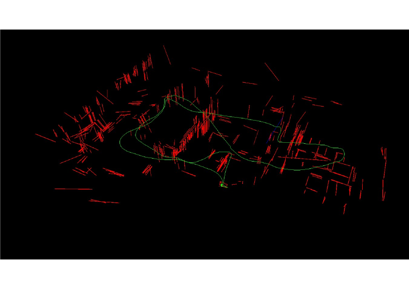
Figure 8: Line feature map generation by IDLL on MH-05-difficult.

V Experiments

In this section, we use the public benchmark datasets, i.e., the EuRoc MAV Dataset[17] to evaluate algorithm performances. Our IDLL method as shown in Fig.9 is compared with three state-of-the-art monocular VIO methods to validate its advantages. The three compared methods are VINS-Mono[14](Point-based methods), PL-VINS[16] and PL-VIO[7] (Point and line-based methods). All of the experiments were performed on a computer with an Intel Core i7-11700 with 2.50GHz, and implemented on Ubuntu 18.04 with ROS Melodic. The screen window is shown as Fig.9.

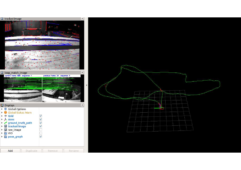
Figure 9: The screen window when running IDLL.

V-A Accuracy Performance

We use two indexes, i.e., the root mean square error (RMSE) of the absolute trajectory error (ATE) and the relative pose error (RPE) to test the localization accuracy of the compared methods. The open-source package EVO (https://michaelgrupp.github.io/evo/) provides an easy-to-use interface to evaluate the trajectories of odometry and SLAM algorithms.

ATE comparison: We test the medium and difficult sequences in EuRoc datasets which include 7 sequences. Table II shows the results of root mean square error (RMSE) of different algorithms. This indicator mainly evaluates the matching accuracy of frame to map, that is, the result of sliding window optimization. From Table II, we can conclude that:

TABLE II: RMSE ATE [M] Comparison of different methods

Datasets	w/o loop				w/ loop
	VINS-Mono	PL-VIO	PL-VINS	IDLL	VINS-Mono	PL-VINS	IDLL
MH-03-Medium	0.236	0.263	0.231	0.204$(\downarrow 11.7\%)$	0.104	0.099	0.071$(\downarrow 28.3\%)$
MH-04-Difficult	0.376	0.360	0.282	0.270$(\downarrow 4.26\%)$	0.220	0.202	0.170$(\downarrow 15.8\%)$
MH-05-Difficult	0.295	0.279	0.272	0.239$(\downarrow 12.1\%)$	0.242	0.226	0.137$(\downarrow 39.4\%)$
V1-02-Medium	0.169	Fail	0.123	0.112$(\downarrow 8.94\%)$	0.091	0.079	0.073$(\downarrow 7.59\%)$
V1-03-Difficult	0.251	0.187	0.182	0.170$(\downarrow 6.59\%)$	0.225	0.180	0.141$(\downarrow 21.7\%)$
V2-02-Medium	0.166	0.156	0.151	0.113$(\downarrow 25.2\%)$	0.139	0.133	0.074$(\downarrow 44.4\%)$
V2-03-Difficult	0.297	0.270	0.237	0.225$(\downarrow 5.60\%)$	0.215	0.196	0.143$(\downarrow 27.0\%)$

• IDLL yields better localization accuracy in medium and difficult environments. For example, the ATE of our method can be as much as $28.2\%(0.376\to 0.270)$ less than that of VINS-Mono on the MH-04-difficult sequence. This shows that the point-line combination approach can indeed increase the number of features extracted in the case of weak texture and low illumination, thus improving SLAM accuracy. Also our method is $4.3\%(0.282\to 0.270)$ accurate than PL-VINS, which shows that the inverse depth representation of line features is indeed more robust than the orthonormal representation.

• loop closure (loop) is a necessary step to eliminate accumulative error, which works on all the seven sequences. Taking VINS-Mono as an example, ATE is reduced from 0.376 to 0.220 on the MH-04-difficult sequence by using loop closure.

RPE comparison: In relative pose error estimation, we also test the medium and difficult sequences in EuRoc dataset, which consist of seven sequences. Table III and Table IV show the results of different algorithms. RPE includes two parts: translational error and rotational error. This index mainly evaluates the matching accuracy from frame to frame. It reveals the performance of frame relative pose optimization, which has a close relationship with the initial triangulation performance of the line features.

From Table III and Table IV, we can conclude that:

• IDLL yields better performance than the other three methods in terms of the RPE performance. However, since IDLL discards two degrees of freedom, it can be seen that the estimation of rotation is not as good as that of translation.

• All point line methods can detect about $2\times 10^{2}$ line features per frame, but only about $1\times 10^{2}$ of them have completed the initialization of line features in our method, which are added to the back-end optimization. However, only about $5\times 10^{1}$ line features can be retained when using the Plücker matrix initialization. This makes the line segments we participate in the calculation more abundant and the results more accurate.

TABLE III: RMSE RPE [M] or [RAD] Comparison of different methods Without Loop

Datasets	w/o loop
	VINS-Mono		PL-VIO		PL-VINS		IDLL
	Trans.	Rot.	Trans.	Rot.	Trans.	Rot.	Trans.	Rot.
MH-03-Medium	0.01174	0.00206	0.006935	0.000456	0.006569	0.000433	0.006388	0.000471
MH-04-Difficult	0.01258	0.001431	0.011454	0.001274	0.008322	0.000871	0.00722	0.000456
MH-05-Difficult	0.01145	0.001048	0.007189	0.000544	0.007174	0.000321	0.006675	0.000333
V1-02-Medium	0.012745	0.00278	Fail	Fail	0.01197	0.001598	0.005159	0.0019277
V1-03-Difficult	0.126693	0.00193	0.00597	0.002394	0.007986	0.006758	0.006186	0.003094
V2-02-Medium	0.013071	0.002729	0.115221	0.002006	0.004547	0.000658	0.004209	0.000938
V2-03-Difficult	0.126455	0.002271	0.012743	0.0054	0.006894	0.002344	0.006122	0.002287

TABLE IV: RMSE RPE [M] or [RAD] Comparison of different methods With Loop

Datasets	w/ loop
	VINS-Mono		PL-VINS		IDLL
	Trans.	Rot.	Trans.	Rot.	Trans.	Rot.
MH-03-Medium	0.013592	0.002459	0.010582	0.001157	0.009249	0.000678
MH-04-Difficult	0.01521	0.001806	0.017375	0.002498	0.009842	0.000954
MH-05-Difficult	0.01601	0.000823	0.020025	0.002436	0.014695	0.001394
V1-02-Medium	0.010025	0.002839	0.011136	0.004869	0.009248	0.001629
V1-03-Difficult	0.134445	0.002084	0.009435	0.003023	0.007862	0.007036
V2-02-Medium	0.125121	0.002058	0.006793	0.003306	0.005904	0.002136
V2-03-Difficult	0.132729	0.002382	0.011246	0.005627	0.010067	0.004776

MH-03-Medium                   MH-05-Difficult                   V1-02-Medium                   V2-03-Difficult

VINS-MONO

(a)

(b)

(c)

(d)

PL-VIO

(e)

(f)

(g)

(h)

PL-VINS

(i)

(j)

(k)

(l)

IDLL

(m)

(n)

(o)

(p)

Figure 10: Comparison of the proposed method. The four colorful trajectories of the first row are run with VINS-Mono on the (a) MH-03-medium; (b) MH-05-difficult; (c) V1-02-medium; and (d) V2-03-difficult sequences. The second row is run with PL-VIO. The third row is run with PL-VINS and the last row is our method(IDLL). Colors encodethe corresponding absolute pose errors.

To demonstrate the results intuitively, several trajectories estimated by IDLL and other methods are shown in Fig.10. The trajectories are colored by heat-map of translation errors. The redder the color is, the larger the translation error is. Comparing trajectories obtained by three methods, we can conclude that IDLL with line features gives the smallest errors comparing with that of the other methods even when the camera was moving with rapid rotations. Furthermore, we found that these sequences with rapid rotation cause large changes in the viewing directions, and the lighting conditions are especially challenging for tracking the point features.

V-B Calculation efficiency Comparison

TABLE V: Thread Time(ms) Comparison of different methods

Method	PL-VIO		PL-VINS		IDLL
	Thread 1 Times	Thread 2 Times	Thread 1 Times	Thread 2 Times	Thread 1 Times	Thread 2 Times
Mean	100	48	46	46	46	36.4

In the part, we compare the computation times of different methods. We also use all EuRoc datasets to calculate the result. “Rate” denotes the pose update frequency whose value is determined by the highest execution time in Thread 2(VIO). We follow the real-time criterion in VINS-Mono which is that if the system can run at over 10 Hz pose update frequency while providing accurate localization information as output. The results are listed in TableV.

In our experiments, IDLL and PL-VINS are both able to run at 10 Hz while PL-VIO fails. Note that IDLL and PL-VINS need $\sim 46ms$ in Thread 1(Line Detection and Tracking) and PL-VIO needs $\sim 100ms$ in Thread 1. Compared with PL-VINS, IDLL is more efficient by using the inverse depth representation in Thread 2(VIO) as shown in TableVI. As we can see, our algorithm can detect more line segment features, but we optimize fewer line parameters, and the time required for back-end optimization in the sliding window is less. So our method(IDLL) is more efficient.

TABLE VI: Average Execution Time(ms) Comparison of different methods

Method	PL-VIO			PL-VINS			IDLL
	Line Num	Line Params	Times	Line Num	Line Params	Times	Line Num	Line Params	Times
Mean	$\sim 5\times 10^{1}$	4	48	$\sim 5\times 10^{1}$	4	46	$\sim 1\times 10^{2}$	2	36.4$(\downarrow 20.87\%)$

VI Conclusion

In this paper, we propose a novel tightly coupled monocular vision-inertial SLAM algorithm IDLL, which optimizes the system state in a sliding window using both point and line features. To efficiently represent the line features, each line feature is represented by the inverse depths of two end-points. This compact representation reduces the parameter numbers during initialization and optimization. We in particular present the inverse depth based initialization, residue function setup, and sliding window based optimization process. In addition, the Jacobian matrix of the line feature residual error terms is given in detail in order to efficiently solve the optimization problem for sliding windows. A two-step optimization method is proposed to solve the optimization problem in the sliding window. The proposed IDLL method is compared to three state-of-the-art monocular VIO methods including VINS-Mono, PL-VIO and PL-VINS on the EuRoc dataset. Based on the analysis and results, we see that the inverse depth line features can greatly help to improve the translation and rotation accuracy of the VIO system, especially in challenging scenes. Comparing with existing point-line based methods, IDLL improves the efficiency to meet the real-time performances and also improves the accuracy in challenging cases. In the future, we plan to improve our system and reconstruct the indoor map by introducing the inverse depth line features in 3D space.

Appendix

Line Measurement Jacobians

The jacobians for the line measurements are as follows:

$$\begin{gathered}\frac{{\partial{r_{l}}}}{{\partial\mathbf{l}}}=\left[{\begin{array}[]{*{20}{l}}{\frac{{\partial{r_{1}}}}{{\partial{l_{1}}}}}&{\frac{{\partial{r_{1}}}}{{\partial{l_{2}}}}}&{\frac{{\partial{r_{1}}}}{{\partial{l_{3}}}}}\\ {\frac{{\partial{r_{2}}}}{{\partial{l_{1}}}}}&{\frac{{\partial{r_{2}}}}{{\partial{l_{2}}}}}&{\frac{{\partial{r_{2}}}}{{\partial{l_{3}}}}}\end{array}}\right]\hfill\\ =\frac{1}{{{{({l_{1}}^{2}+{l_{2}}^{2})}^{\frac{1}{2}}}}}{\left[{\begin{array}[]{*{20}{l}}{\frac{{-{l_{1}}{s_{{c_{j}}}}^{\top}\mathbf{l}}}{{({l_{1}}^{2}+{l_{2}}^{2})}}+{u_{s}}}&{\frac{{-{l_{2}}{s_{{c_{j}}}}^{\top}\mathbf{l}}}{{({l_{1}}^{2}+{l_{2}}^{2})}}+{v_{s}}}&1\\ {\frac{{-{l_{1}}{e_{{c_{j}}}}^{\top}\mathbf{l}}}{{({l_{1}}^{2}+{l_{2}}^{2})}}+{u_{e}}}&{\frac{{-{l_{2}}{e_{{c_{j}}}}^{\top}\mathbf{l}}}{{({l_{1}}^{2}+{l_{2}}^{2})}}+{v_{e}}}&1\end{array}}\right]_{2\times 3}}\hfill\\ \end{gathered}$$ (18)

$$\frac{{\partial\mathbf{l}}}{{\partial{L_{{c_{j}}}}}}={\left[{\begin{array}[]{*{20}{c}}{\mathbf{K_{L}}}&{{0_{3}}}\end{array}}\right]_{3\times 6}},\mathbf{K_{L}}=\left[{\begin{array}[]{*{20}{c}}{{f_{y}}}&0&0\\ 0&{{f_{x}}}&0\\ {-{f_{y}}{c_{x}}}&{-{f_{x}}{c_{y}}}&{{f_{x}}{f_{y}}}\end{array}}\right]$$ (19)

To compute the line re-projection error, a spatial line in camera frame $c_{i}$ is transformed to the body frame $b_{i}$ with the extrinsic parameters $\mathbf{T}_{bc}$ firstly, and then transformed to the world frame $w$. Next, we transform the space line to the body frame $b_{j}$, finally to camera frame $c_{j}$.

$${L_{{c_{j}}}}={\mathbf{T}_{bc}}^{-1}{\mathbf{T}_{w{b_{j}}}}^{-1}{\mathbf{T}_{w{b_{i}}}}{\mathbf{T}_{bc}}{L_{{c_{i}}}}$$ (20)

The Jacobian matrix of the line re-projection error with respect to rotation and position of the j-th IMU body state is:

$$\frac{{\partial{\mathbf{L}_{{c_{j}}}}}}{{\partial{\theta\delta_{{b_{j}}}}}} ={\mathbf{T}_{bc}}^{-1}\left[{\begin{array}[]{*{20}{c}}{\frac{{\partial(I-{{\left[{\delta{\theta_{{b_{j}}}}}\right]}_{\times}})\mathbf{R}_{w{b_{j}}}^{\top}({\mathbf{n}_{w}}+{{\left[{{\mathbf{d}_{w}}}\right]}_{\times}}{\mathbf{t}_{w{b_{j}}}})}}{{\partial{\theta\delta_{{b_{j}}}}}}}\\ {\frac{{\partial(I-{{\left[{\delta{\theta_{{b_{j}}}}}\right]}_{\times}})\mathbf{R}_{w{b_{j}}}^{\top}{\mathbf{d}_{w}}}}{{\partial{\theta\delta_{{b_{j}}}}}}}\end{array}}\right]$$ (21)

$$={\mathbf{T}_{bc}}^{-1}{\left[{\begin{array}[]{*{20}{c}}{{{\left[{\mathbf{R}_{w{b_{j}}}^{\top}({\mathbf{n}_{w}}+{{\left[{{\mathbf{d}_{w}}}\right]}_{\times}}{\mathbf{t}_{w{b_{j}}}})}\right]}_{\times}}}\\ {{{\left[{\mathbf{R}_{w{b_{j}}}^{\top}{\mathbf{d}_{w}}}\right]}_{\times}}}\end{array}}\right]_{6\times 3}}$$

$$\frac{{\partial{L_{{c_{j}}}}}}{{\partial\delta{t_{{b_{j}}}}}} ={\mathbf{T}_{bc}}^{-1}\left[{\begin{array}[]{*{20}{c}}{\frac{{\partial\mathbf{R}_{w{b_{j}}}^{\top}({\mathbf{n}_{w}}+{{\left[{{\mathbf{d}_{w}}}\right]}_{\times}}({\mathbf{t}_{w{b_{j}}}}+\delta{t_{{b_{j}}}}))}}{{\partial\delta{t_{{b_{j}}}}}}}\\ {\frac{{\partial\mathbf{R}_{w{b_{j}}}^{\top}{\mathbf{d}_{w}}}}{{\partial\delta{t_{{b_{j}}}}}}}\end{array}}\right]$$ (22)

$$={\mathbf{T}_{bc}}^{-1}{\left[{\begin{array}[]{*{20}{c}}{\mathbf{R}_{w{b_{j}}}^{\top}{{\left[{{\mathbf{d}_{w}}}\right]}_{\times}}}\\ 0\end{array}}\right]_{6\times 3}}$$

The Jacobian matrix of the line re-projection error with respect to rotation and position of the i-th IMU body state and the extrinsic parameters also can get in a similar way.

The Jacobian matrix of the line re-projection error respect to the inverse depth representation is:

$$\frac{{\partial{L_{{c_{i}}}}}}{{\partial\delta l}} =\left[{\begin{array}[]{*{20}{c}}{\frac{{\partial{\mathbf{n}_{{c_{i}}}}}}{{\partial\delta{\lambda_{s}}}}}&{\frac{{\partial{\mathbf{d}_{{c_{i}}}}}}{{\partial\delta{\lambda_{s}}}}}\\ {\frac{{\partial{\mathbf{n}_{{c_{i}}}}}}{{\partial\delta{\lambda_{e}}}}}&{\frac{{\partial{\mathbf{d}_{{c_{i}}}}}}{{\partial\delta{\lambda_{e}}}}}\end{array}}\right]$$ (23)

$$=\left[{\begin{array}[]{*{20}{c}}{-\frac{1}{{{\lambda_{s}}^{2}{\lambda_{e}}}}{s_{{c_{i}}}}\times{e_{{c_{i}}}}}&{\frac{1}{{{\lambda_{s}}^{2}}}{s_{{c_{i}}}}}\\ {-\frac{1}{{{\lambda_{e}}^{2}{\lambda_{s}}}}{s_{{c_{i}}}}\times{e_{{c_{i}}}}}&{-\frac{1}{{{\lambda_{e}}^{2}}}{e_{{c_{i}}}}}\end{array}}\right]$$

Proof of Two-step Minimization

Let us denote as $r$ the value of cost of Equation 15 at the k-th iteration. At the (k + 1)-th iteration, we first minimize $r_{l}$ in Equation 15 with the fixed poses and obtained at the k-th iteration. Assume the value of Equation 15 after this step is $r_{k+1}^{\left[1\right]}$. As the other terms in Equation 15 do not involve the 3D lines, they keep the same value after this step. Thus it is clear that $r_{k+1}^{[1]}\leqslant{r_{k+1}}$. In the second step, we fix the value of inverse depths of 3D lines and conduct one LM step for the poses to reduce the value of $r_{k+1}^{[1]}$. Assume the value of Equation 15 after this step is $r_{k+1}$. It is obvious that

$$0\leqslant{r_{k+1}}\leqslant r_{k+1}^{[1]}\leqslant{r_{k}}$$ (24)

According to the monotone convergence theorem (i.e., if a sequence is decreasing and bounded below, this sequence has a limit), the two-step minimization algorithm always converges.

Appendix A Biography Section

Wanting Li is a PhD student in the Department of Computer Science, Renmin University of China. She received the BS degree in Computer science and technology from China Agricultural University (2019). She won Honorable Mentions in 2018 mathematical modeling contest of American College Students. Her research is unsupervised learning in pervasive computing.

Yu Shao is a master student in the Department of Computer Science, Renmin University of China. He received the BS degree in Computer science and technology from Renmin University of China (2021). His research interest is lidar SLAM (Simultaneous Localization and Mapping) algorithms.

Yongcai Wang received his BS and PhD degrees from department of automation sciences and engineering, Tsinghua University in 2001 and 2006 respectively. He worked as associated researcher at NEC Labs. China from 2007-2009. He was an research scientist in Institute for Interdisciplinary Information Sciences (IIIS), Tsinghua University from 2009-2015. He was a visiting scholar at Cornell University in 2015. He is currently associate professor at Department of Computer Sciences, Renmin University of China. His research interests include network localization and crowdsourcing based mapping.

Shuo Wang received the BS degree from the School of Information, Renmin University of China, where he is pursuing the PhD degree. His research interests include network localization algorithms, graph optimization, and applications.

Xuewei Bai received the BS degree from the Department of Computer Science and Technology, North China Electric Power University, in 2020. She is currently working toward the PhD degree in the Department of Computer Sciences, Renmin University of China. Her research interests include network localization algorithms and graph optimization and applications.

Deying Li received the MS degree in Mathematics from Huazhong Normal University (1988) and PhD degree in Computer Science from City University of Hong Kong (2004). She is currently a Professor in the Department of Computer Science, Renmin University of China. Her research includes wireless networks, mobile computing, social network and algorithm design and analysis.

References

- [1] P. D. Groves, “Principles of gnss, inertial, and multisensor integrated navigation systems, [book review],” IEEE Aerospace and Electronic Systems Magazine, vol. 30, no. 2, pp. 26–27, 2015.
- [2] G. Retscher and A. Kealy, “Ubiquitous positioning technologies for modern intelligent navigation systems,” The Journal of Navigation, vol. 59, no. 1, pp. 91–103, 2006.
- [3] X. Wang and J. Wang, “Detecting glass in simultaneous localisation and mapping,” Robotics and Autonomous Systems, vol. 88, pp. 97–103, 2017.
- [4] J. Gui, D. Gu, S. Wang, and H. Hu, “A review of visual inertial odometry from filtering and optimisation perspectives,” Advanced Robotics, vol. 29, no. 20, pp. 1289–1301, 2015.
- [5] T. Naseer, G. L. Oliveira, T. Brox, and W. Burgard, “Semantics-aware visual localization under challenging perceptual conditions,” in ICRA 2017, 2017, pp. 2614–2620.
- [6] N. Piasco, D. Sidibé, V. Gouet-Brunet, and C. Demonceaux, “Learning scene geometry for visual localization in challenging conditions,” in 2019 International Conference on Robotics and Automation (ICRA). IEEE, 2019, pp. 9094–9100.
- [7] Y. He, J. Zhao, Y. Guo, W. He, and K. Yuan, “Pl-vio: Tightly-coupled monocular visual–inertial odometry using point and line features,” Sensors, vol. 18, no. 4, p. 1159, 2018.
- [8] Y. Yang, P. Geneva, K. Eckenhoff, and G. Huang, “Visual-inertial navigation with point and line features,” Macau, China, Nov, 2019.
- [9] S. Leutenegger, S. Lynen, M. Bosse, R. Siegwart, and P. Furgale, “Keyframe-based visual–inertial odometry using nonlinear optimization,” The International Journal of Robotics Research, vol. 34, no. 3, pp. 314–334, 2015.
- [10] R. Mur-Artal and J. D. Tardós, “Visual-inertial monocular slam with map reuse,” IEEE Robotics and Automation Letters, vol. 2, no. 2, pp. 796–803, 2017.
- [11] C. Campos, R. Elvira, J. J. G. Rodríguez, J. M. Montiel, and J. D. Tardós, “Orb-slam3: An accurate open-source library for visual, visual–inertial, and multimap slam,” IEEE Transactions on Robotics, vol. 37, no. 6, pp. 1874–1890, 2021.
- [12] A. Concha, G. Loianno, V. Kumar, and J. Civera, “Visual-inertial direct slam,” in 2016 IEEE international conference on robotics and automation (ICRA). IEEE, 2016, pp. 1331–1338.
- [13] R. G. Von Gioi, J. Jakubowicz, J.-M. Morel, and G. Randall, “Lsd: A fast line segment detector with a false detection control,” IEEE transactions on pattern analysis and machine intelligence, vol. 32, no. 4, pp. 722–732, 2008.
- [14] T. Qin, P. Li, and S. Shen, “Vins-mono: A robust and versatile monocular visual-inertial state estimator,” IEEE Transactions on Robotics, vol. 34, no. 4, pp. 1004–1020, 2018.
- [15] P. Geneva, K. Eckenhoff, W. Lee, Y. Yang, and G. Huang, “Openvins: A research platform for visual-inertial estimation,” in 2020 IEEE International Conference on Robotics and Automation (ICRA). IEEE, 2020, pp. 4666–4672.
- [16] Q. Fu, J. Wang, H. Yu, I. Ali, F. Guo, Y. He, and H. Zhang, “Pl-vins: Real-time monocular visual-inertial slam with point and line features,” arXiv preprint arXiv:2009.07462, 2020.
- [17] M. Burri, J. Nikolic, P. Gohl, T. Schneider, J. Rehder, S. Omari, M. W. Achtelik, and R. Siegwart, “The euroc micro aerial vehicle datasets,” The International Journal of Robotics Research, vol. 35, no. 10, pp. 1157–1163, 2016.
- [18] J. Engel, V. Koltun, and D. Cremers, “Direct sparse odometry,” IEEE transactions on pattern analysis and machine intelligence, vol. 40, no. 3, pp. 611–625, 2017.
- [19] J. Engel, T. Schöps, and D. Cremers, “Lsd-slam: Large-scale direct monocular slam,” in European conference on computer vision. Springer, 2014, pp. 834–849.
- [20] C. Forster, M. Pizzoli, and D. Scaramuzza, “Svo: Fast semi-direct monocular visual odometry,” in 2014 IEEE international conference on robotics and automation (ICRA). IEEE, 2014, pp. 15–22.
- [21] L. Zhou, S. Wang, and M. Kaess, “Dplvo: Direct point-line monocular visual odometry,” IEEE Robotics and Automation Letters, vol. 6, no. 4, pp. 7113–7120, 2021.
- [22] L. Zhou, G. Huang, Y. Mao, S. Wang, and M. Kaess, “Edplvo: Efficient direct point-line visual odometry,” in 2022 International Conference on Robotics and Automation (ICRA). IEEE, 2022, pp. 7559–7565.
- [23] G. Klein and D. Murray, “Parallel tracking and mapping for small ar workspaces,” in 2007 6th IEEE and ACM international symposium on mixed and augmented reality. IEEE, 2007, pp. 225–234.
- [24] R. Mur-Artal, J. M. M. Montiel, and J. D. Tardos, “Orb-slam: a versatile and accurate monocular slam system,” IEEE transactions on robotics, vol. 31, no. 5, pp. 1147–1163, 2015.
- [25] A. Pumarola, A. Vakhitov, A. Agudo, A. Sanfeliu, and F. Moreno-Noguer, “Pl-slam: Real-time monocular visual slam with points and lines,” in 2017 IEEE international conference on robotics and automation (ICRA). IEEE, 2017, pp. 4503–4508.
- [26] R. Mur-Artal and J. D. Tardós, “Orb-slam2: An open-source slam system for monocular, stereo, and rgb-d cameras,” IEEE transactions on robotics, vol. 33, no. 5, pp. 1255–1262, 2017.
- [27] A. I. Mourikis, S. I. Roumeliotis et al., “A multi-state constraint kalman filter for vision-aided inertial navigation.” in ICRA, vol. 2, 2007, p. 6.
- [28] K. Wu, A. M. Ahmed, G. A. Georgiou, and S. I. Roumeliotis, “A square root inverse filter for efficient vision-aided inertial navigation on mobile devices.” in Robotics: Science and Systems, vol. 2. Rome, Italy, 2015.
- [29] M. K. Paul, K. Wu, J. A. Hesch, E. D. Nerurkar, and S. I. Roumeliotis, “A comparative analysis of tightly-coupled monocular, binocular, and stereo vins,” in 2017 IEEE International Conference on Robotics and Automation (ICRA). IEEE, 2017, pp. 165–172.
- [30] M. Bloesch, S. Omari, M. Hutter, and R. Siegwart, “Robust visual inertial odometry using a direct ekf-based approach,” in 2015 IEEE/RSJ international conference on intelligent robots and systems (IROS). IEEE, 2015, pp. 298–304.
- [31] L. Von Stumberg, V. Usenko, and D. Cremers, “Direct sparse visual-inertial odometry using dynamic marginalization,” in 2018 IEEE International Conference on Robotics and Automation (ICRA). IEEE, 2018, pp. 2510–2517.
- [32] Y. Yang, P. Geneva, X. Zuo, K. Eckenhoff, Y. Liu, and G. Huang, “Tightly-coupled aided inertial navigation with point and plane features,” in 2019 International Conference on Robotics and Automation (ICRA). IEEE, 2019, pp. 6094–6100.
- [33] Y. Zhang, R. Jin, and Z.-H. Zhou, “Understanding bag-of-words model: a statistical framework,” International journal of machine learning and cybernetics, vol. 1, no. 1, pp. 43–52, 2010.
- [34] S. Leutenegger, M. Chli, and R. Y. Siegwart, “Brisk: Binary robust invariant scalable keypoints,” in 2011 International conference on computer vision. Ieee, 2011, pp. 2548–2555.
- [35] J. Shi et al., “Good features to track,” in 1994 Proceedings of IEEE conference on computer vision and pattern recognition. IEEE, 1994, pp. 593–600.
- [36] C. Harris, M. Stephens et al., “A combined corner and edge detector,” in Alvey vision conference, vol. 15, no. 50. Manchester, UK, 1988, pp. 10–5244.
- [37] V. Usenko, N. Demmel, D. Schubert, J. Stückler, and D. Cremers, “Visual-inertial mapping with non-linear factor recovery,” IEEE Robotics and Automation Letters, vol. 5, no. 2, pp. 422–429, 2019.
- [38] A. Rosinol, M. Abate, Y. Chang, and L. Carlone, “Kimera: an open-source library for real-time metric-semantic localization and mapping,” in 2020 IEEE International Conference on Robotics and Automation (ICRA). IEEE, 2020, pp. 1689–1696.
- [39] E. Rublee, V. Rabaud, K. Konolige, and G. Bradski, “Orb: An efficient alternative to sift or surf,” in 2011 International conference on computer vision. Ieee, 2011, pp. 2564–2571.
- [40] T. Sattler, B. Leibe, and L. Kobbelt, “Fast image-based localization using direct 2d-to-3d matching,” in 2011 International Conference on Computer Vision. IEEE, 2011, pp. 667–674.
- [41] J. L. Schönberger, T. Price, T. Sattler, J.-M. Frahm, and M. Pollefeys, “A vote-and-verify strategy for fast spatial verification in image retrieval,” in Asian Conference on Computer Vision. Springer, 2016, pp. 321–337.
- [42] S. Baker and I. Matthews, “Lucas-kanade 20 years on: A unifying framework,” International journal of computer vision, vol. 56, no. 3, pp. 221–255, 2004.
- [43] L. Zhang and R. Koch, “An efficient and robust line segment matching approach based on lbd descriptor and pairwise geometric consistency,” Journal of Visual Communication and Image Representation, vol. 24, no. 7, pp. 794–805, 2013.
- [44] M. Joswig and T. Theobald, Plücker Coordinates and Lines in Space. London: Springer London, 2013, pp. 193–207. [Online]. Available: https://doi.org/10.1007/978-1-4471-4817-3_12
- [45] Y. Yang and G. Huang, “Observability analysis of aided ins with heterogeneous features of points, lines, and planes,” IEEE Transactions on Robotics, vol. 35, no. 6, pp. 1399–1418, 2019.
- [46] C. Chen, B. Wang, C. X. Lu, N. Trigoni, and A. Markham, “A survey on deep learning for localization and mapping: Towards the age of spatial machine intelligence,” arXiv preprint arXiv:2006.12567, 2020.
- [47] W. Chen, G. Shang, A. Ji, C. Zhou, X. Wang, C. Xu, Z. Li, and K. Hu, “An overview on visual slam: From tradition to semantic,” Remote Sensing, vol. 14, no. 13, p. 3010, 2022.
- [48] R. Hartley and A. Zisserman, Multiple view geometry in computer vision. Cambridge university press, 2003.
- [49] A. Kaehler and G. Bradski, Learning OpenCV 3: computer vision in C++ with the OpenCV library. ” O’Reilly Media, Inc.”, 2016.
- [50] C. Forster, L. Carlone, F. Dellaert, and D. Scaramuzza, “On-manifold preintegration for real-time visual–inertial odometry,” IEEE Transactions on Robotics, vol. 33, no. 1, pp. 1–21, 2016.
- [51] G. Zhang, J. H. Lee, J. Lim, and I. H. Suh, “Building a 3-d line-based map using stereo slam,” IEEE Transactions on Robotics, vol. 31, no. 6, pp. 1364–1377, 2015.
- [52] “https://mathworld.wolfram.com/plane.html.”
- [53] R. Rosipal, “Nonlinear partial least squares an overview,” Chemoinformatics and advanced machine learning perspectives: complex computational methods and collaborative techniques, pp. 169–189, 2011.
- [54] J. L. Schonberger and J.-M. Frahm, “Structure-from-motion revisited,” in Proceedings of the IEEE conference on computer vision and pattern recognition, 2016, pp. 4104–4113.
- [55] S. Shen, N. Michael, and V. Kumar, “Tightly-coupled monocular visual-inertial fusion for autonomous flight of rotorcraft mavs,” in 2015 IEEE International Conference on Robotics and Automation (ICRA). IEEE, 2015, pp. 5303–5310.
- [56] J. Civera, A. J. Davison, and J. M. Montiel, “Inverse depth parametrization for monocular slam,” IEEE transactions on robotics, vol. 24, no. 5, pp. 932–945, 2008.
- [57] T. Qin, P. Li, and S. Shen, “Relocalization, global optimization and map merging for monocular visual-inertial slam,” in 2018 IEEE International Conference on Robotics and Automation (ICRA). IEEE, 2018, pp. 1197–1204.
- [58] V. Lepetit, F. Moreno-Noguer, and P. Fua, “Epnp: An accurate o (n) solution to the pnp problem,” International journal of computer vision, vol. 81, no. 2, pp. 155–166, 2009.
Acknowledgments
This should be a simple paragraph before the References to thank those individuals and institutions who have supported your work on this article.