Sarah Frank-Wolfe: Method for Constrained Optimization with Best Rates and Practical Features

Sarah Frank-Wolfe: Methods for Constrained Optimization with Best Rates and Practical Features

Abstract

The Frank-Wolfe (FW) method is a popular approach for solving optimization problems with structured constraints that arise in machine learning applications. In recent years, stochastic versions of FW have gained popularity, motivated by large datasets for which the computation of the full gradient is prohibitively expensive. In this paper, we present two new variants of the FW algorithms for stochastic finite-sum minimization. Our algorithms have the best convergence guarantees of existing stochastic FW approaches for both convex and non-convex objective functions. Our methods do not have the issue of permanently collecting large batches, which is common to many stochastic projection-free approaches. Moreover, our second approach does not require either large batches or full deterministic gradients, which is a typical weakness of many techniques for finite-sum problems. The faster theoretical rates of our approaches are confirmed experimentally.

1 Introduction

Empirical risk minimization is a cornerstone for training supervised machine learning models such as various regressions, support vector machine, and neural networks [Shalev-Shwartz and Ben-David, 2014]. We consider a constrained problem of this type:

$$\min_{x\in\mathcal{X}\subset\mathbb{R}^{d}}f(x)=\frac{1}{n}\sum\limits_{i=1}^{n}f_{i}(x)\,.$$ (1)

The objective function of (1) has the form of a finite sum. Typically, this setting corresponds to the sum of the losses of the model with parameters $x$ applied to a large number of data points, indexed by $i=1,\ldots,n$. Because $n$ is large, calculating the full gradient of $f$ is expensive. Therefore, stochastic methods which very rarely resort to calling $\nabla f$ (or avoid it altogether) are of particular importance. In this problem setting, we assume the set $\mathcal{X}\subset\mathbb{R}^{d}$ to be convex, that projecting onto this set is expensive, and that it also admits a fast linear minimization oracle (LMO).

The study of methods for (1) that do not require projections has a history of more than half a century. Arguably the most popular projection-free method is the Frank-Wolfe (a.k.a, Conditional Gradient algorithm [Frank and Wolfe, 1956]). This method maintains sparse iterates and only requires a linear minimization oracle that takes into account the specificity of the constraint set $\mathcal{X}$. In particular, the classical version of the method considers a linear approximation of the function at the current point $x^{k}$, and minimizes this approximation on the set $\mathcal{X}$:

$$\begin{split}s^{k}&=\arg\min_{s\in\mathcal{X}}\langle\nabla f(x^{k}),s-x^{k}\rangle,\\ x^{k+1}&=x^{k}+\eta_{k}(s^{k}-x^{k}),\end{split}$$ (2)

where $\eta_{k}$ is parameter-free and equal to $\tfrac{2}{k+2}$.

In the last decade, the Frank-Wolfe-type approaches have attracted increasing interest in the machine-learning community because of their good performance on sparse problems, or on problems where the constraints are complex but structured (e.g., various $\ell_{p}$ balls, trace norms), having applications to submodular optimization [Bach, 2011], vision [Miech et al., 2017, Bojanowski et al., 2014], and variational inference [Krishnan et al., 2015].

Due to the significant increase in dataset size and complexity within the machine learning community, stochastic algorithms are of great interest and are the focus of this paper. In particular, we seek to answer the two following questions:

1. Can we improve upon the convergence rates of existing approaches for Eq. 1?
2. Can we avoid the computation of both full gradients and large batches of stochastic gradients?

2 Related works and our contributions

Table 1: Summary of the results on projection free methods for stochastic constrained minimization problems.

Reference	Convex case complexity		Non-convex case complexity		No full gradients?	No big batches?
	SFO	LMO	SFO	LMO
Frank and Wolfe [1956](1) [Lacoste-Julien, 2016](1)	${\cal O}\left(\frac{n}{\varepsilon}\right)$	${\cal O}\left(\frac{1}{\varepsilon}\right)$	${\cal O}\left(\frac{n}{\varepsilon^{2}}\right)$	${\cal O}\left(\frac{1}{\varepsilon^{2}}\right)$	✗	✗
Hazan and Kale [2012]	$\mathcal{O}\left(\frac{1}{\varepsilon^{4}}\right)$	$\mathcal{O}\left(\frac{1}{\varepsilon^{2}}\right)$	✗		✓	✗
Lan and Zhou [2016]	$\mathcal{O}\left(\frac{1}{\varepsilon^{2}}\right)$	$\mathcal{O}\left(\frac{1}{\varepsilon}\right)$	✗		✓	✗
Reddi et al. [2016] Alg. 2	✗		$\mathcal{O}\left(\frac{1}{\varepsilon^{4}}\right)$	$\mathcal{O}\left(\frac{1}{\varepsilon^{2}}\right)$	✓	✗
Reddi et al. [2016] Alg. 3	✗		$\mathcal{O}\left(n+\frac{n^{2/3}}{\varepsilon^{2}}\right)$	$\mathcal{O}\left(\frac{1}{\varepsilon^{2}}\right)$	✗	✗
Reddi et al. [2016] Alg. 4	✗		$\mathcal{O}\left(\frac{n}{\varepsilon^{2}}\right)$ (2)	$\mathcal{O}\left(\frac{1}{\varepsilon^{2}}\right)$	✗	✗
Hazan and Luo [2016]	$\mathcal{\tilde{O}}\left(n+\frac{1}{\varepsilon^{2}}\right)$	$\mathcal{O}\left(\frac{1}{\varepsilon}\right)$	✗		✗	✗
Qu et al. [2018] Alg. 3	✗		$\mathcal{O}\left(\frac{1}{\varepsilon^{4}}\right)$ (3)	$\mathcal{O}\left(\frac{1}{\varepsilon^{4}}\right)$ (3)	✓	✗
Qu et al. [2018] Alg. 4	✗		$\mathcal{O}\left(n+\frac{n^{2/3}}{\varepsilon^{2}}\right)$ (3)	$\mathcal{O}\left(\frac{1}{\varepsilon^{4}}\right)$ (3)	✗	✗
Yurtsever et al. [2019]	$\mathcal{O}\left(\frac{1}{\varepsilon^{2}}\right)$	$\mathcal{O}\left(\frac{1}{\varepsilon}\right)$	$\mathcal{O}\left(\frac{\sqrt{n}}{\varepsilon^{2}}\right)$	$\mathcal{O}\left(\frac{1}{\varepsilon^{2}}\right)$	✗	✗
Gao and Huang [2020] Alg. 1	✗		$\mathcal{O}\left(\frac{\sqrt{n}}{\varepsilon^{2}}\right)$	$\mathcal{O}\left(\frac{1}{\varepsilon^{2}}\right)$	✗	✗
Gao and Huang [2020] Alg. 2	✗		$\mathcal{O}\left(\frac{\sqrt{n}}{\varepsilon^{2}}\right)$ (3)	$\mathcal{O}\left(\frac{1}{\varepsilon^{4}}\right)$ (3)	✗	✗
Mokhtari et al. [2020]	${\cal O}\left(\frac{1}{\varepsilon^{3}}\right)$	${\cal O}\left(\frac{1}{\varepsilon^{3}}\right)$	✗		✓	✓
Négiar et al. [2020](4)	${\cal O}\left(\frac{n}{\varepsilon}\right)$ (5)	${\cal O}\left(\frac{n}{\varepsilon}\right)$ (5)	convergence without rate		✓	✓
Lu and Freund [2021](4)	${\cal O}\left(\frac{n}{\varepsilon}\right)$	${\cal O}\left(\frac{n}{\varepsilon}\right)$	✗		✓	✓
Akhtar and Rajawat [2021]	${\cal O}\left(\frac{1}{\varepsilon^{2}}\right)$	${\cal O}\left(\frac{1}{\varepsilon^{2}}\right)$	✗		✓	✓
Weber and Sra [2022] Alg.2	$\mathcal{O}\left(\frac{1}{\varepsilon^{4}}\right)$	$\mathcal{O}\left(\frac{1}{\varepsilon^{2}}\right)$	$\mathcal{O}\left(\frac{1}{\varepsilon^{4}}\right)$	$\mathcal{O}\left(\frac{1}{\varepsilon^{2}}\right)$	✓	✗
Weber and Sra [2022] Alg.3	$\mathcal{O}\left(n+\frac{n^{2/3}}{\varepsilon^{2}}\right)$	$\mathcal{O}\left(\frac{1}{\varepsilon^{2}}\right)$	$\mathcal{O}\left(n+\frac{n^{2/3}}{\varepsilon^{2}}\right)$	$\mathcal{O}\left(\frac{1}{\varepsilon^{2}}\right)$	✗	✗
Weber and Sra [2022] Alg.4	$\mathcal{O}\left(\frac{1}{\varepsilon^{3}}\right)$	$\mathcal{O}\left(\frac{1}{\varepsilon^{2}}\right)$	$\mathcal{O}\left(\frac{1}{\varepsilon^{3}}\right)$	$\mathcal{O}\left(\frac{1}{\varepsilon^{2}}\right)$	✓	✗
Hou et al. [2022]	${\cal O}\left(\frac{1}{\varepsilon^{2}}\right)$	${\cal O}\left(\frac{1}{\varepsilon^{2}}\right)$	${\cal O}\left(\exp\left(\frac{1}{\varepsilon}\right)\right)$	${\cal O}\left(\exp\left(\frac{1}{\varepsilon}\right)\right)$	✓	✓
(This paper) Alg. 1	$\mathcal{\tilde{O}}\left(n+\frac{\sqrt{n}}{\varepsilon}\right)$	$\mathcal{\tilde{O}}\left(\sqrt{n}+\frac{1}{\varepsilon}\right)$	$\mathcal{O}\left(\frac{\sqrt{n}}{\varepsilon^{2}}\right)$	$\mathcal{O}\left(\frac{1}{\varepsilon^{2}}\right)$	✗	✗
(This paper) Alg. 1	$\mathcal{\tilde{O}}\left(n+\frac{\sqrt{n}}{\varepsilon}\right)$	$\mathcal{\tilde{O}}\left(n+\frac{\sqrt{n}}{\varepsilon}\right)$	$\mathcal{O}\left(\frac{n}{\varepsilon^{2}}\right)$	$\mathcal{O}\left(\frac{n}{\varepsilon^{2}}\right)$	✗	✓
(This paper) Alg. 2	$\mathcal{\tilde{O}}\left(n+\frac{\sqrt{n}}{\varepsilon}\right)$	$\mathcal{\tilde{O}}\left(\sqrt{n}+\frac{1}{\varepsilon}\right)$	$\mathcal{O}\left(\frac{\sqrt{n}}{\varepsilon^{2}}\right)$	$\mathcal{O}\left(\frac{1}{\varepsilon^{2}}\right)$	✓	✗
(This paper) Alg. 2	$\mathcal{\tilde{O}}\left(n+\frac{\sqrt{n}}{\varepsilon}\right)$	$\mathcal{\tilde{O}}\left(n+\frac{\sqrt{n}}{\varepsilon}\right)$	$\mathcal{O}\left(\frac{n}{\varepsilon^{2}}\right)$	$\mathcal{O}\left(\frac{n}{\varepsilon^{2}}\right)$	✓	✓

• ⁽¹⁾ fully deterministic; ⁽²⁾ the authors give a different complexity, but it seems to us that their proof contains an error, we try to correct it (see Appendix C.2); ⁽³⁾ in the original papers, the authors give better results, e.g. $\mathcal{O}(\nicefrac{{\sqrt{n}}}{{\varepsilon}})$ instead of $\mathcal{O}(\nicefrac{{\sqrt{n}}}{{\varepsilon^{2}}})$, but this results violate the lower bounds (see Table 1 from Li et al. [2021a]]), this is due to the difference in the convergence criterion: in Li et al. [2021a], the authors use $\|\nabla f\|^{2}\sim\varepsilon^{2}$ and in Qu et al. [2018], Gao and Huang [2020] – $\|\nabla f\|^{2}\sim\varepsilon$; ⁽⁴⁾ only for linear models; ⁽⁵⁾ the authors give a rate in the form $\kappa/\varepsilon$, where $\kappa$ is a special constant, which is equal to $n$ in the worst case. Notation: $\varepsilon$ = accuracy of the solution, $n$ = size of the dataset, SFO = stochastic first-order oracle, LMO = linear minimization oracle.

After Frank and Wolfe [1956] proposed the FW algorithm, many works improved its theory and extended it to special cases Levitin and Polyak [1966], Demianov and Rubinov [1970], Dunn and Harshbarger [1978], Patriksson [1993]. About ten years ago, Jaggi [2013], Lacoste-Julien and Jaggi [2015] developed more robust and practical versions of the original FW method, motivated by ML applications with sparsity and structured constraints (see Braun et al. [2022] for a detailed historical survey).

Motivated by applications with large datasets, the theory of stochastic methods for unconstrained (or projection-friendly) optimization problems has built upon the highly successful SGD method [Robbins and Monro, 1951, Nemirovski et al., 2009] to obtain faster methods for finite sum-problems. Particularly, many so-called variance-reduced variants of SGD have been proposed, including SAG/SAGA [Defazio et al., 2014, Schmidt et al., 2017, Qian et al., 2019], SVRG [Johnson and Zhang, 2013, Allen-Zhu and Yuan, 2016, Yang et al., 2021], MISO [Mairal, 2015], SARAH [Nguyen et al., 2017a, 2021, b, Hu et al., 2019, Li et al., 2021b], SPIDER [Fang et al., 2018], STORM [Cutkosky and Orabona, 2019], PAGE [Li et al., 2021a], and many others.

Extensive research in the theory of deterministic Frank-Wolfe-type methods and stochastic methods for unconstrained problems has led to the development of stochastic versions of projection-free algorithms. Hazan and Kale [2012] proposed an algorithm for online stochastic optimization. Lan and Zhou [2016] developed a projection-free version of using sliding. Hazan and Luo [2016], Reddi et al. [2016], Qu et al. [2018], Yurtsever et al. [2019], Gao and Huang [2020], Shen et al. [2019] proposed modifications of the Frank-Wolfe method using variance reduction techniques, namely SVRG, SAGA and SPIDER. Mokhtari et al. [2020], Akhtar and Rajawat [2021], Hou et al. [2022] used the idea of momentum to deal with stochasticity. Négiar et al. [2020] and Lu and Freund [2021] explored stochastic methods for linear predictors. Weber and Sra [2022] extended the results of Reddi et al. [2016] from convex sets to manifolds. We summarize and compare the convergence rate of each method in Tabel 1. Note that for the SAGA-related methods, we report a slightly different result from the one reported by Reddi et al. [2016] because we believe that their proof contains a slight inaccuracy (see App. C.2) for more details. We also do not include the approach from [Shen et al., 2019] in Tabel 1, since this method uses the hessian of the target function.

Next, we detail our contributions which can be divided into four parts.

$\bullet$ The best rates in the convex case. Our convergence guarantees are better than the classical deterministic method [Frank and Wolfe, 1956] as well as the stochastic methods from [Négiar et al., 2020, Lu and Freund, 2021, Weber and Sra, 2022] in terms of dataset size $n$. Moreover, the theoretical rates of our methods also surpasses the rest existing results from [Hazan and Kale, 2012, Lan and Zhou, 2016, Hazan and Luo, 2016, Yurtsever et al., 2019, Gao and Huang, 2020, Mokhtari et al., 2020, Akhtar and Rajawat, 2021, Weber and Sra, 2022] in terms of the accuracy $\varepsilon$.

$\bullet$ No need for full gradients. Many stochastic methods, especially for finite-sum problems, require the calculation of some full gradients. This makes these techniques less practical because even the infrequent computation of the deterministic gradient can slow down the convergence. Some methods for constrained problems also have this disadvantage [Reddi et al., 2016, Hazan and Luo, 2016, Qu et al., 2018, Yurtsever et al., 2019, Gao and Huang, 2020, Weber and Sra, 2022]. While Algorithm 1 also requires the computation of the full gradient, Algorithm 2 removes this issue and uses only stochastic gradients. Note that this modification does not affect convergence: Algorithm 1 and Algorithm 2 have the same theoretical guarantees.

$\bullet$ Small batches. Many methods that avoid the computation of the full gradient still use large fixed batch sizes [Hazan and Kale, 2012, Lan and Zhou, 2016, Reddi et al., 2016, Qu et al., 2018, Gao and Huang, 2020, Weber and Sra, 2022] or batch sizes that geometrically increase with iteration number [Hazan and Luo, 2016, Yurtsever et al., 2019], which, like with the collection of full gradients, is a rather strong limitation on the practical applicability of the method. Conversely, our algorithms are guaranteed to converge with all sizes of batches. Large batches are only required to get a slightly better dependence in $n$ for the non-convex case. Methods dealing with fixed small batches are either only analyzed for linear predictors [Négiar et al., 2020, Lu and Freund, 2021], or have slower convergence rates than our approach [Mokhtari et al., 2020, Akhtar and Rajawat, 2021, Hou et al., 2022].

$\bullet$ Non-convex analysis. We give convergence results not only for the convex problem, but also in the case where the target function $f$ in (1) is non-convex. In this setting, our oracle complexity results are the first to be non-exponential (in $\epsilon$) with small mini-batches, and are state-of-the-art with large mini-batches.

3 Notation and Assumptions

We use $\langle x,y\rangle=\sum_{i=1}^{d}x_{i}y_{i}$ to denote the standard inner product of vectors $x,y\in\mathbb{R}^{d}$, where $x_{i}$ corresponds to the $i$-th component of $x$ in the standard basis in $\mathbb{R}^{n}$. With this notation we can introduce the standard $\ell_{2}$-norm in $\mathbb{R}^{d}$ in the following way: $\|x\|=\sqrt{\langle x,x\rangle}$. We write $[n]=\{1,2,\dots,n\}$. Calls of the stochastic oracle means computing the gradient $\nabla f_{i}$ for some $i\in[n]$.

In order to prove convergence results, we state the following standard assumptions on the problem (1). The first two assumptions relate to the target function $f$, and the third relates to the constraint set $\mathcal{X}$.

We start with the assumption that the gradients of both the function $f$ and all terms $\{f_{i}\}^{n}_{i=1}$ are smooth. This assumption is standard in the optimization literature and widely used in the analysis of Frank-Wolfe-type methods.

Assumption 3.1.

The function $f:\mathcal{X}\to\mathbb{R}$, is $L$-smooth on $\mathcal{X}$, i.e., there exists a constant $L>0$ such that

$$\|\nabla f(x)-\nabla f(y)\|\leq L\|x-y\|\,,\quad\forall\,x,y\in\mathcal{X}.$$

Each function $f_{i}:\mathcal{X}\to\mathbb{R}$, $i\in[n]$, is $L_{i}$-smooth on $\mathcal{X}$, i.e., there exists a constant $L_{i}>0$ such that,

$$\|\nabla f_{i}(x)-\nabla f_{i}(y)\|\leq L_{i}\|x-y\|\,,\quad\forall\,x,y\in\mathcal{X}.$$

We also define the constant $\tilde{L}$ as $\tilde{L}^{2}:=\tfrac{1}{n}\sum_{i=1}^{n}L_{i}^{2}$. By convexity of $x\mapsto x^{2}$, it is easy to prove that $\tilde{L}\geq L$.

Algorithm 1 Sarah Frank-Wolfe

Parameters: step sizes $\{\eta_{k}\}_{k\geq 0}$, probability $p$, batch size $b$;
      Initialization: choose $x^{0}\in\mathcal{X}$; $g^{0}=\nabla f(x^{0})$;

1:for $k=0,1,2,\ldots K-1$ do

2:     Compute $s^{k}=\arg\min_{s\in\mathcal{X}}\langle g^{k},s\rangle$;

3:     Update $x^{k+1}=x^{k}+\eta_{k}(s^{k}-x^{k})$ with $\eta_{k}$

4:     Generate batch $S_{k}$ with size $b$;

5:     Update $g^{k+1}=\begin{cases}\nabla f(x^{k+1}),&\text{with probability }p,\\ g^{k}+\frac{1}{b}\sum\limits_{i\in S_{k}}[\nabla f_{i}(x^{k+1})-\nabla f_{i}(x^{k})],&\text{with probability }1-p,\end{cases}$;

6:end for

The second assumption is the convexity of the function $f$.

Assumption 3.2.

The function $f:\mathcal{X}\to\mathbb{R}$, is convex, i.e.,

$$f(x)\geq f(y)+\langle\nabla f(y),x-y\rangle,\,\quad\forall\,x,y\in\mathcal{X}.$$

Note that we consider both convex and non-convex cases of the function $f$. But even if $f$ is convex, we do not additionally assume that the terms $\{f_{i}\}_{i=1}^{n}$ are convex, hence in general they can be non-convex. Naturally, it is common to find settings with convex $f$ and convex $f_{i}$, but formulations with non-convex $f_{i}$ also arise, e.g., in PCA [Garber and Hazan, 2015, Shamir, 2015, Allen-Zhu and Yuan, 2016]. This phenomenon is also believed occur in neural networks [Allen-Zhu and Hazan, 2016, Johnson and Zhang, 2013].

The next assumption is also typical and found in all works on projection-free methods.

Assumption 3.3.

The set $\mathcal{X}$ is convex and compact with a diameter $D$, i.e., for any $x,y\in\mathcal{X}$,

$$\|x-y\|\leq D.$$

4 Main part

In this section, we present two new algorithms and their convergence guarantees.

4.1 State-of-the-art complexity with Sarah Frank-Wolfe

Previously, Reddi et al. [2016], Hazan and Luo [2016], Weber and Sra [2022] proposed to modify the classical Frank-Wolfe algorithm (2) using the SVRG technique [Johnson and Zhang, 2013]. The essence of these modifications is to change the deterministic gradient in the Conditional Gradient method to some stochastic gradient $g^{k}$, e.g., calculated according to the SVRG approach:

$$g^{k}=\nabla f_{i_{k}}(x^{k})-\nabla f_{i_{k}}(w^{k})+\nabla f(w^{k}),$$

where $i_{k}$ is randomly generated from $[n]$, and $w^{k}$ is rarely taken equal to $x^{k}$ rather than $w^{k-1}$. Therefore, when we update $w^{k}=x^{k}$, we sometimes need to consider the full deterministic gradient. The update rule for $w^{k}$ can be deterministic (as in the original version) or randomized, known as the loopless approach [Kovalev et al., 2020]. Meanwhile, there are other variance-reduced methods, such as SARAH [Nguyen et al., 2017a]:

$$g^{k}=\nabla f_{i_{k}}(x^{k})-\nabla f_{i_{k}}(x^{k-1})+g^{k-1},$$ (3)

where $i_{k}$ is also randomly generated from $[n]$, and $g^{k}$ is rarely taken equal to $\nabla f(x^{k})$ rather than (3).

As noted in the original paper on SARAH, this method has better convergence guarantees and smoother convergence paths with less oscillations than SVRG, making SARAH preferred in both theory and practice. As a result, we use SARAH (specifically the loopless version [Li et al., 2021a]) as a base for Algorithm 1. First we give the convergence of Algorithm 1 in the convex case.

Theorem 4.1.

Let $\{x^{k}\}_{k\geq 0}$ denote the iterates of Algorithm 1 for solving problem (1), which satisfies Assumptions 3.1–3.3. Let $x^{*}$ be the minimizer of $f$. Then for any $K$ one can choose $\{\eta_{k}\}_{k\geq 0}$ as follows:

$$\text{if}~{}~{}K\leq\frac{2}{p}, \eta_{k}=\frac{p}{2},$$

$$\text{if}~{}~{}K>\frac{2}{p}~{}~{}\text{ and }~{}~{}k<\left\lceil\frac{K}{2}\right\rceil, \eta_{k}=\frac{p}{2},$$

$$\text{if}~{}~{}K>\frac{2}{p}~{}~{}\text{ and }~{}~{}k\geq\left\lceil\frac{K}{2}\right\rceil, \eta_{k}=\frac{2}{(\nicefrac{{4}}{{p}}+k-\lceil\nicefrac{{K}}{{2}}\rceil)}.$$

For this choice of $\eta_{k}$, we have the following convergence:

$$\mathbb{E}\left[f(x^{K})-f(x^{*})\right]=\mathcal{O}\Bigg{(}\frac{f(x^{0})-f(x^{*})}{p}\exp\left(-\frac{Kp}{4}\right)+\left[1+\frac{\tilde{L}}{L}\sqrt{\frac{1-p}{pb}}\right]\frac{LD^{2}}{K}\Bigg{)}.$$

Algorithm 2 Saga Sarah Frank-Wolfe

Parameters: step sizes $\{\eta_{k}\}_{k\geq 0}$; momentum $\lambda$; batch size $b$;
      Initialization: choose $x^{0}\in\mathcal{X}$; $g^{0}=\nabla f(x^{0})$ or $g^{0}=\nabla f_{i_{0}}(x^{0})$; $y^{0}_{i}=\nabla f_{i}(x^{0})$ or $y^{0}_{i}=0$ for $i\in[n]$;

1:for $k=0,1,2,\ldots K-1$ do

2:     Compute $s^{k}=\arg\min_{s\in\mathcal{X}}\langle g^{k},s\rangle$;

3:     Update $x^{k+1}=x^{k}+\eta_{k}(s^{k}-x^{k})$ with $\eta_{k}$

4:     Generate batch $S_{k}$ with size $b$

5:     Update $g^{k+1}=\frac{1}{b}\sum\limits_{i\in S_{k}}[\nabla f_{i}(x^{k+1})-\nabla f_{i}(x^{k})]+(1-\lambda)g^{k}+\lambda\left(\frac{1}{b}\sum\limits_{i\in S_{k}}[\nabla f_{i}(x^{k})-y^{k}_{i}]+\frac{1}{n}\sum\limits_{j=1}^{n}y_{j}^{k}\right)$;

6:     Update $y^{k+1}_{i}=\begin{cases}\nabla f_{i}(x^{k+1}),&i\in S_{k},\\ y^{k}_{i},&i\notin S_{k},\end{cases}$;

7:end for

See the full proof in Section B.1. To choose $p$, one can note that for each iteration, we on average compute the stochastic gradient $(pn+(1-p)\cdot 2b)$ times: with probability $p$ we need the full gradient, with probability $(1-p)$ – a batch of size $b$ in two points $x^{k+1}$ and $x^{k}$. If we take $p$ close to $1$, the guarantees in Theorem 4.1 gives faster convergence, but the oracle complexity per iteration increases. For example, if we take $p=1$, we simply obtain a deterministic method, and the estimates for convergence and the number of gradient calculations reproduce the results for the classical Frank-Wolfe method. On the other hand, if $p$ tends to $0$, the number of stochastic gradient calls per iteration decreases, but the iterative convergence rate drops. It is optimal to choose $p$ based on the condition: $pn=2(1-p)b$, i.e. $p=\tfrac{2b}{n+2b}$. From Theorem 4.1 we can also obtain an estimate on the required number of linear minimizations (LMO complexity). It is equal to the number of iterations of Algorithm 1. Then, the following corollary holds.

Corollary 4.2.

Under the conditions of Theorem 4.1, Algorithm 1 with $p=\tfrac{2b}{n+2b}$ achieves an $\varepsilon$ suboptimality with

$$\mathcal{O}\left(\frac{n}{b}\log\frac{1}{\varepsilon}+\left[1+\frac{\tilde{L}\sqrt{n}}{bL}\right]\frac{LD^{2}}{\varepsilon}\right)\;\text{LMO calls, and}$$

$$\mathcal{O}\left(n\log\frac{1}{\varepsilon}+\left[b+\frac{\tilde{L}\sqrt{n}}{L}\right]\frac{LD^{2}}{\varepsilon}\right)\,\text{stochastic oracle calls.}$$

For any $b\leq\tfrac{\tilde{L}\sqrt{n}}{L}$, the estimate of the number of calls for the stochastic oracles does not change. Given that $\tilde{L}\geq L$, the smallest batch size $b=1$ is appropriate for us. In this setting, the required number of the stochastic gradient computations is $\mathcal{\tilde{O}}\left(n+\tfrac{\sqrt{n}\tilde{L}D^{2}}{\varepsilon}\right)$. This result is the best in the literature, especially since it does not require using large batches (see Table 1). For $p=\tfrac{2b}{n+2b}$ and $b=\sqrt{n}$, the LMO complexity is $\mathcal{\tilde{O}}\left(\sqrt{n}+\tfrac{\tilde{L}D^{2}}{\varepsilon}\right)$, this result is optimal (see Section 2.1.2 from [Braun et al., 2022]). With $b=1$, the LMO complexity equals $\mathcal{\tilde{O}}\left(n+\tfrac{\sqrt{n}\tilde{L}D^{2}}{\varepsilon}\right)$. Note that for many practical examples, the LMO complexity is not the computational bottleneck since the solution of linear minimization problems has a closed-form solution (see, e.g., Algorithm 2 from [Bellet et al., 2015]). It is also important to notice that, based on the above choices for $\eta_{k}$, $p$, and $b$, both our method and the original Frank-Wolfe are independent of the objective function parameters (e.g., $L$ or $\tilde{L}$).

Next, we prove the convergence of Algorithm 1 for the non-convex objective function $f$. We use the Frank-Wolfe gap function [Jaggi, 2013] as a criterion for convergence:

$$\operatorname{gap}(y)=\max_{x\in\mathcal{X}}\,\langle\nabla f(y),y-x\rangle.$$ (4)

Such a criterion is standard in the analysis of algorithms for the constrained problems with non-convex functions [Lacoste-Julien, 2016, Reddi et al., 2016]. It is easy to check that $\operatorname{gap}(y)\geq 0$ for any $y\in\mathcal{X}$. Moreover, a point $y\in X$ is stationary for (1) if and only if $\operatorname{gap}(y)=0$. Lacoste-Julien [2016] notes that the Frank-Wolfe gap is a meaningful measure of non-stationarity, and also an affine invariant generalization of the more standard convergence criterion $\|\nabla f(y)\|$ that is used for unconstrained non-convex problems. Then the following theorem is valid.

Theorem 4.3.

Let $\{x^{k}\}_{k\geq 0}$ denote the iterates of Algorithm 1 for solving problem (1), which satisfies Assumptions 3.1,3.3. Let $x^{*}$ be the global (may be not unique) minimizer of $f$. Then, if we choose $\eta_{k}=\frac{1}{\sqrt{K}}$, we have the following convergence:

$$\mathbb{E}\left[\min_{0\leq k\leq K-1}\operatorname{gap}(x^{k})\right]=\mathcal{O}\left(\frac{f(x^{0})-f(x^{*})}{\sqrt{K}}+\frac{LD^{2}}{\sqrt{K}}\left[1+\frac{\tilde{L}}{L}\sqrt{\frac{(1-p)}{pb}}\right]\right).$$

See the proof in Section B.2. In this case, the optimal choice of the parameter $p$ is the same as in Corollary 4.2 of Theorem 4.1.

Corollary 4.4.

Under the conditions of Theorem 4.3, Algorithm 1 with $p=\tfrac{2b}{n+2b}$ achieves an $\varepsilon$ suboptimality with

$$\mathcal{O}\left(\left[\frac{h^{0}}{\varepsilon}\right]^{2}+\left[\frac{LD^{2}}{\varepsilon}\right]^{2}\left[1+\frac{\tilde{L}^{2}n}{L^{2}b^{2}}\right]\right)\;\text{LMO calls, and}$$

$$\mathcal{O}\left(b\left[\frac{h^{0}}{\varepsilon}\right]^{2}+\left[\frac{LD^{2}}{\varepsilon}\right]^{2}\left[b+\frac{\tilde{L}^{2}n}{L^{2}b}\right]\right)\,\text{stochastic oracle calls,}$$

where $h^{0}:=f(x^{0})-f(x^{*}).$

First, we substitute $b=1$ in the previous result. This gives us an oracle complexity of $\mathcal{O}\left(\tfrac{n\tilde{L}^{2}D^{4}}{\varepsilon^{2}}\right)$, which corresponds to the Frank-Wolfe complexity. If we choose the batch size $b=\tfrac{\sqrt{n}\tilde{L}}{L}$ that minimizes the expression $\left[b+\tfrac{\tilde{L}^{2}n}{L^{2}b}\right]$, then we need $\mathcal{O}\left(\tfrac{\sqrt{n}\tilde{L}LD^{4}}{\varepsilon^{2}}\right)$ stochastic gradient calls. If one wishes to avoid using $\tilde{L}$ and $L$ constants when selecting $b$, it is possible to take $b=\sqrt{n}$, and the complexity then becomes $\mathcal{O}\left(\tfrac{\sqrt{n}\tilde{L}^{2}D^{4}}{\varepsilon^{2}}\right)$. As noted earlier, both of these estimates are the best result of the projection-free methods for non-convex constrained problems (see Table 1). Additionally, with $p=\tfrac{2b}{n+2b}$ and $b=1$, the LMO complexity is equal to $\mathcal{O}\left(\tfrac{n\tilde{L}^{2}D^{4}}{\varepsilon^{2}}\right)$, and with $b=\sqrt{n}$, it is $\mathcal{O}\left(\tfrac{\tilde{L}^{2}D^{4}}{\varepsilon^{2}}\right)$.

4.2 Avoiding full gradient computations with Saga Sarah Frank-Wolfe

The idea of Algorithm 2 is to use a combination [Li et al., 2021b] of the SARAH and SAGA [Defazio et al., 2014] approaches. Both SAGA and SARAH are some of the main variance-reduced methods for finite-sum minimization problems. An important feature of SAGA is that it does not use full gradient calculations, but it has worse convergence guarantees than SARAH (see, e.g., Table 2 in [Nguyen et al., 2017a]). The synergy of SARAH and SAGA brings together the strengths of both methods.

The essence of the SAGA method is similar to SVRG, but where SVRG collects the full gradients at some reference points, SAGA instead maintains a "sliding" version of the full gradient. The gradient $\nabla f(w)$ at the reference point $w$ may become obsolete after a small number of iterations, but in the course of the algorithm we compute newer stochastic gradients for some $i\in[n]$, and one can leverage them to calculate a more recent approximation of the full gradient. To do this, SAGA introduces additional vectors $\{y\}_{i=1}^{n}$; each such $y_{i}$ keeps the latest version of the gradient $\nabla f_{i}$ (implemented in line 6). The $\tfrac{1}{n}\sum_{j=1}^{n}y_{j}^{k}$ term is the aforementioned approximation of the full gradient. The calculation of $g^{k}_{\text{SAGA}}$ is $g^{k}_{\text{SAGA}}=\big{(}\tfrac{1}{b}\sum_{i\in S_{k}}[\nabla f_{i}(x^{k})-y^{k}_{i}]+\tfrac{1}{n}\sum_{j=1}^{n}y_{j}^{k}\big{)}$ (similarly to SVRG and SARAH). Line 5 provides a combination of $g^{k}_{\text{SARAH}}$ and $g^{k}_{\text{SAGA}}$.

Recall that the average number of the stochastic oracle calls per iteration of Algorithm 1 is $(pn+(1-p)\cdot 2b)$, and that Algorithm 2 requires $2b$ computations of the stochastic gradients each iteration. In lines 5 and 6, one need to calculate $\nabla f_{i}(x^{k+1})$, $\nabla f_{i}(x^{k})$ for $i\in S_{k}$. Therefore, if $b\leq\tfrac{n}{2}$, then for any $p\neq 0$, the complexity of one iteration of Algorithm 2 is better than that of Algorithm 1.

In summary, Algorithm 2 does not collect full gradients and has a bit better iteration complexity, but is required to use $n$ extra vectors $\{y_{i}\}_{i=1}^{n}$, requiring an additional $\mathcal{O}(nd)$ memory cost compared to Algorithm 1. Oce can note that the methods from [Négiar et al., 2020, Lu and Freund, 2021] also use an extra memory size of $\mathcal{O}(nd)$.

For the convex target function $f$, Algorithm 2 satisfies the following convergence theorem.

Theorem 4.5.

Let $\{x^{k}\}_{k\geq 0}$ denote the iterates of Algorithm 2 for solving problem (1), which satisfies Assumptions 3.1–3.3. Let $x^{*}$ be the minimizer of $f$. Then for any $K$ one can choose $\{\eta_{k}\}_{k\geq 0}$ as follows:

$$\text{if}~{}~{}K\leq\frac{4n}{b}, \eta_{k}=\frac{b}{4n},$$

$$\text{if}~{}~{}K>\frac{4n}{b}~{}~{}\text{ and }~{}~{}k<\left\lceil\frac{K}{2}\right\rceil, \eta_{k}=\frac{b}{4n},$$

$$\text{if}~{}~{}K>\frac{4n}{b}~{}~{}\text{ and }~{}~{}k\geq\left\lceil\frac{K}{2}\right\rceil, \eta_{k}=\frac{2}{(\nicefrac{{8n}}{{b}}+k-\lceil\nicefrac{{K}}{{2}}\rceil)},$$

and $\lambda=\tfrac{b}{2n}$. For this choice of $\eta_{k}$ and $\lambda$, we have the following convergence:

$$\mathbb{E}\left[f(x^{K})-f(x^{*})\right]={\cal O}\Bigg{(}\frac{n\left[f(x^{0})-f(x^{*})\right]}{b}\exp\left(-\frac{bK}{8n}\right)+\left[1+\frac{\tilde{L}\sqrt{n}}{Lb}\right]\frac{LD^{2}}{K}\Bigg{)}.$$

See the proof in Section B.3. Since we do not need to choose $p$ for Algorithm 2 we proceed directly to the corollary on the oracle complexity.

Corollary 4.6.

Under the conditions of Theorem 4.5, Algorithm 2 achieves an $\varepsilon$ suboptimality with

$$\mathcal{O}\left(\frac{n}{b}\log\frac{1}{\varepsilon}+\left[1+\frac{\tilde{L}\sqrt{n}}{bL}\right]\frac{LD^{2}}{\varepsilon}\right)\;\text{LMO calls, and}$$

$$\mathcal{O}\left(n\log\frac{1}{\varepsilon}+\left[b+\frac{\tilde{L}\sqrt{n}}{L}\right]\frac{LD^{2}}{\varepsilon}\right)\,\text{stochastic oracle calls.}$$

This result is exactly the same as Corollary 4.2, so we obtain the same conclusions for choosing the size of $b$ as that Corollary 4.2. In particular, in this case with $b=1$, the method also have oracle complexity $\mathcal{\tilde{O}}\left(n+\tfrac{\sqrt{n}\tilde{L}D^{2}}{\varepsilon}\right)$ – the best among the works on stochastic projection-free methods. The findings on the LMO complexity is also consistent with Theorem 4.1. Note also that Algorithm 2, just the same as Algorithm 1 and the classical Frank-Wolfe method, is free of the target function’s parameters.

In the following theorem for the non-convex case of $f$, as in Theorem 4.3, we use (4) to estimate convergence.

Theorem 4.7.

Let $\{x^{k}\}_{k\geq 0}$ denote the iterates of Algorithm 2 for solving problem (1), which satisfies Assumptions 3.1,3.3. Let $x^{*}$ be the global (may be not unique) minimizer of $f$ on $\mathcal{X}$. Then, if we choose $\eta_{k}=\frac{1}{\sqrt{K}}$ and $\lambda=\tfrac{b}{2n}$, we have the following convergence:

$$\mathbb{E}\left[\min_{0\leq k\leq K-1}\operatorname{gap}(x^{k})\right]=\mathcal{O}\left(\frac{f(x^{0})-f(x^{*})}{\sqrt{K}}+\frac{LD^{2}}{\sqrt{K}}\left[1+\frac{\tilde{L}\sqrt{n}}{Lb}\right]\right).$$

See the proof in Section B.4.

Corollary 4.8.

Under the conditions of Theorem 4.7, Algorithm 2 achieves an $\varepsilon$ suboptimality with

$$\mathcal{O}\left(\left[\frac{h^{0}}{\varepsilon}\right]^{2}+\left[\frac{LD^{2}}{\varepsilon}\right]^{2}\left[1+\frac{\tilde{L}^{2}n}{L^{2}b^{2}}\right]\right)\;\text{LMO calls, and}$$

$$\mathcal{O}\left(b\left[\frac{h^{0}}{\varepsilon}\right]^{2}+\left[\frac{LD^{2}}{\varepsilon}\right]^{2}\left[b+\frac{\tilde{L}^{2}n}{L^{2}b}\right]\right)\,\text{stochastic oracle calls, }$$

where $h^{0}:=f(x^{0})-f(x^{*}).$

We once again have the same results as for Algorithm 1 in Corollary 4.4, resulting in the same analysis for choosing the batch sizes and for the LMO complexity.

5 Experiments

We conduct our experiments on the constrained empirical risk for a linear model with weights $w$ and on training samples $\{x_{i},y_{i}\}_{i=1}^{n}$. Then, the logistic regression problem is

$$\min_{w\in\mathcal{C}}f(w)=\frac{1}{n}\sum\limits_{i=1}^{n}\log(1+\exp(-y_{i}w^{T}x_{i})),$$ (5)

where $y_{i}\in\{-1,1\}$, and the non-linear least squares loss is

$$\min_{w\in\mathcal{C}}f(w)=\frac{1}{n}\sum\limits_{i=1}^{n}(y_{i}-1/(1+\exp(w^{T}x_{i})))^{2},$$ (6)

with $y_{i}\in\{0,1\}$. We consider two different loss functions to test our algorithms on both convex and nonconvex settings. We choose $\mathcal{C}$ as the $\ell_{1}$ norm ball with radius $\lambda=2\cdot 10^{3}$. The LMO for such a constraint set can be computed in a closed-form solution. We take LibSVM [Chang and Lin, 2011] datasets (see Table 2).

For comparison, we consider the methods from Table 1, which do not use large batches: [Mokhtari et al., 2020, Lu and Freund, 2021, Négiar et al., 2020]. Our method is tuned according to the theory (see Sections 4.1 and 4.2), but we take the batchsize $b=\left\lceil\tfrac{n}{100}\right\rceil$ (similarly as the baselines). For the baselines, we use the implementation of Négiar et al. [2020] and tune each method accordingly.

Table 2: Datasets from LibSVM in experiments.

Dataset	$d$	$n$
a9a	123	22696
breast cancer	10	683
madelon	500	2000
mushrooms	112	8124
w8a	300	49749

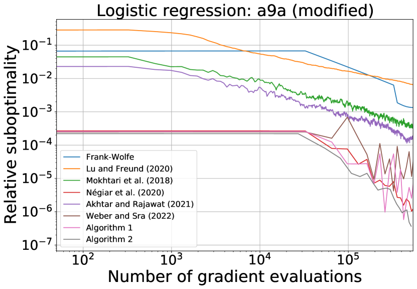
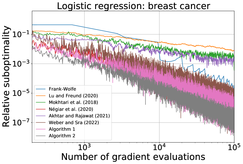
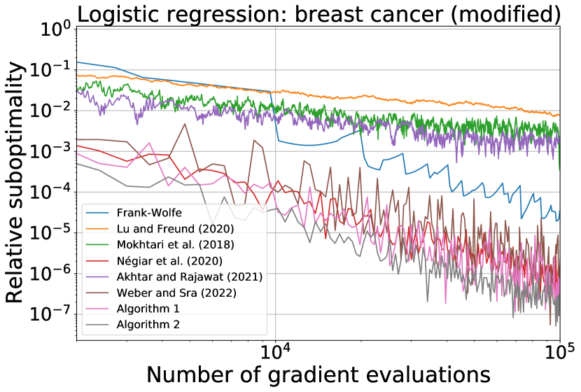
(a) a9a

(b) breast cancer

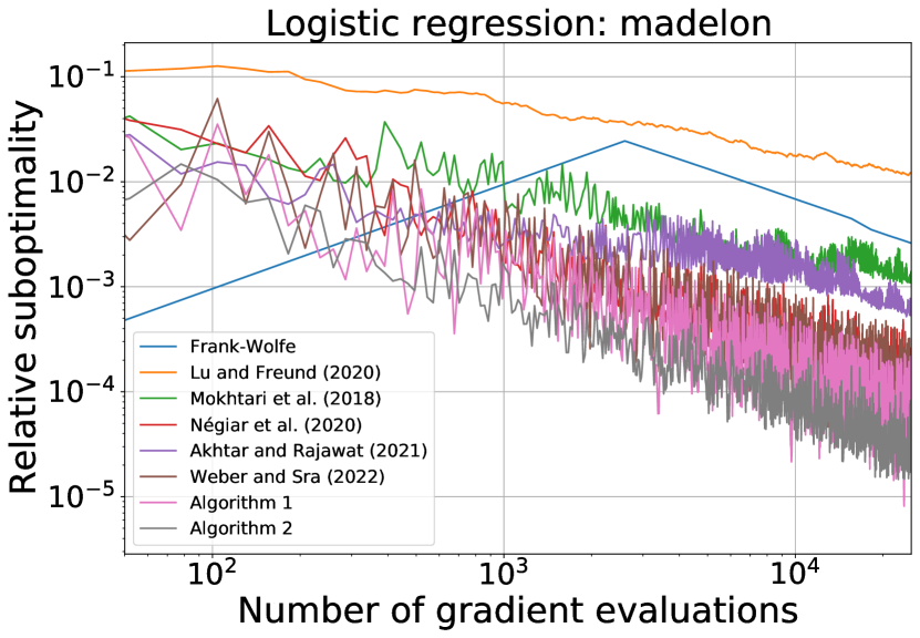
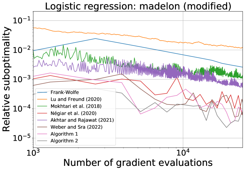
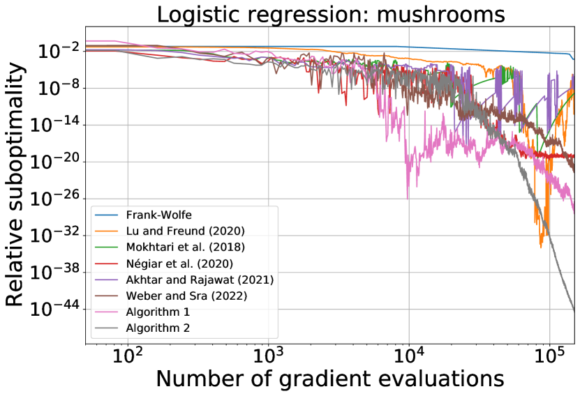
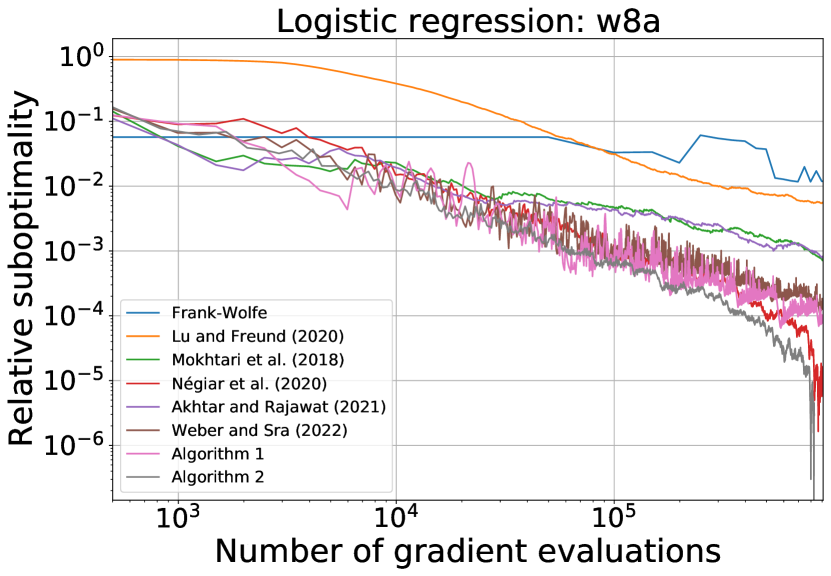
(c) madelon

(d) mushrooms

(e) w8a

Figure 1: Comparison of state-of-the-art projection free methods with small batches for (5). The comparison is made on the real datasets from LibSVM. The criterion is the number of full gradients computations. In the modified plots (the right plots in the first three lines), we left only every 100th point for [Négiar et al., 2020], [Weber and Sra, 2022], Algorithm 1 and Algorithm 2.

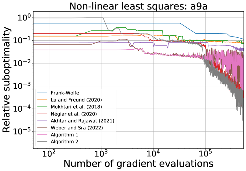
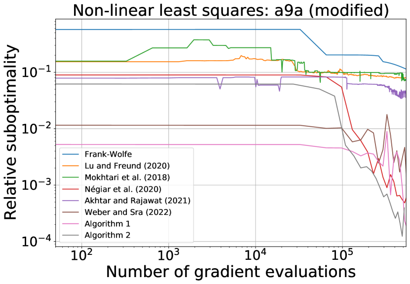
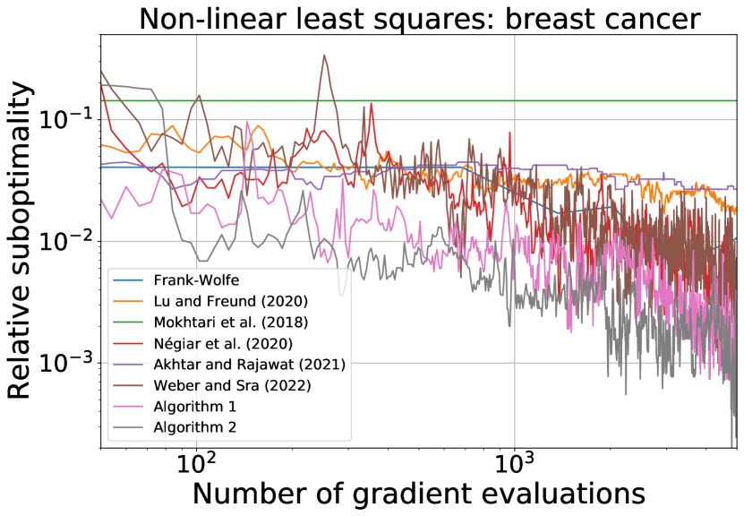
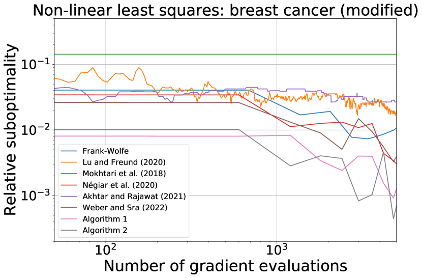
(a) a9a

(b) breast cancer

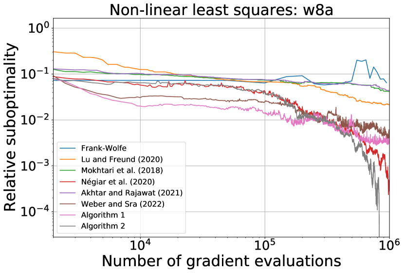
(c) mushrooms

(d) w8a

Figure 2: Comparison of state-of-the-art projection free methods with small batches for (6). The comparison is made on the real datasets from LibSVM. The criterion is the number of full gradients computations. In the modified plots (the right plots in the first three lines), we left only every 100th point for [Négiar et al., 2020], [Weber and Sra, 2022], Algorithm 1 and Algorithm 2.

In Figure 1 we plot the relative suboptimality which is defined a $\nicefrac{{(f(x_{t})-f_{\min})}}{{(f_{\max}-f_{\min})}}$ where $f_{\max}$ is the largest value observed along the optimization and $f_{\min}$ is obtained by running the best algorithm a bit longer than what is plotted. From our results, it is clear that our algorithms are superior or comparable to the baselines, despite the fact that some methods were specifically designed for linear models (e.g. Négiar et al. [2020], Lu and Freund [2021]) which is not the case for Algorithm 1 and 2.

6 Conclusion and future works

In this paper, we presented two new algorithms for stochastic finite-sum optimization. Our methods are based on the Frank-Wolfe and Sarah approaches. Both of our algorithms are free of target function parameters. In both convex and non-convex target cases, our algorithms have the best stochastic oracle complexity in the literature. Our methods do not need to resort to large batch computation. However, in the non-convex case, it is worth noticing that the methods with large batch sizes give a better oracle complexity estimate. Moreover, Algorithm 2 does not need to collect either large batches or full deterministic gradients at all. Our methods also perform well on different $\ell_{1}$ constrained logistic regression problems.

Ideas from Jaggi [2013], and Lacoste-Julien and Jaggi [2015] can be noted as a starting point for future research in order to get frast rates in the strong convex case. The modifications presented in these papers make the Frank-Wolfe method more practical and faster. Combining these and our approaches can produce a strong synergy that results in new practical algorithms.

Finally, the question of obtaining lower bounds for stochastic projection-free methods with linear minimization oracle for constraint sets (in the deterministic case, a lower-bound is known [Jaggi, 2013]) remains open. However, our results in Table 1, match the lower bound given for non-convex unconstrained minimization [Li et al., 2021a, Table 1]). Which seems to indicate that our method is optimal (in terms of stochastic oracle call) for non-convex minimization.

Appendix A Technical facts

Lemma A.1.

For any $x_{1},\ldots,x_{n}\in\mathbb{R}^{d}$ the following inequality holds:

$$\left\|\sum\limits_{i=1}^{n}x_{i}\right\|^{2}\leq n\sum\limits_{i=1}^{n}\|x_{i}\|^{2}.$$

Lemma A.2 (Lemma 1.2.3 from [Nesterov, 2003]).

Suppose that $f$ is $L$-smooth. Then, for any $x,y\in\mathbb{R}^{d}$,

$$f(x)\leq f(y)+\langle\nabla f(y),x-y\rangle+\frac{L}{2}\|x-y\|^{2}.$$

Lemma A.3 (Lemma 3 from [Stich, 2019]).

Let $\{r_{k}\}_{k\geq 0}$ is a non-negative sequence, which satisfies the relation

$$r_{k+1}\leq(1-\eta_{k})r_{k}+c\eta_{k}^{2}.$$

Then there exists stepsizes $\eta_{k}\leq\tfrac{1}{d}$, such that:

$$r_{K}={\cal O}\left(dr_{0}\exp\left(-\frac{K}{2d}\right)+\frac{c}{K}\right).$$

In particular, the step sizes $\{\eta\}_{k\geq 0}$ can be chosen as follows

$$\text{if }~{}~{}K\leq d, \eta_{k}=\frac{1}{d},$$

$$\text{if }~{}~{}K>d~{}~{}\text{ and }~{}~{}k<k_{0}, \eta_{k}=\frac{1}{d},$$

$$\text{if }~{}~{}K>d~{}~{}\text{ and }~{}~{}k\geq k_{0}, \eta_{k}=\frac{2}{(2d+k-k_{0})},$$

where $k_{0}=\lceil\tfrac{K}{2}\rceil$.

Appendix B Missing proofs

B.1 Proof of Theorem 4.1

Theorem B.1 (Theorem 4.1).

Let $\{x^{k}\}_{k\geq 0}$ denote the iterates of Algorithm 1 for solving problem (1), which satisfies Assumptions 3.1–3.3. Let $x^{*}$ be the minimizer of $f$. Then for any $K$ one can choose $\{\eta_{k}\}_{k\geq 0}$ as follows:

$$\text{if}~{}~{}K\leq\frac{2}{p}, \eta_{k}=\frac{p}{2},$$

$$\text{if}~{}~{}K>\frac{2}{p}~{}~{}\text{ and }~{}~{}k<k_{0}, \eta_{k}=\frac{p}{2},$$

$$\text{if}~{}~{}K>\frac{2}{p}~{}~{}\text{ and }~{}~{}k\geq k_{0}, \eta_{k}=\frac{2}{(\nicefrac{{4}}{{p}}+k-\lceil\nicefrac{{K}}{{2}}\rceil)}.$$

For this choice of $\eta_{k}$, we have the following convergence:

$$\mathbb{E}\left[f(x^{K})-f(x^{*})\right]=\mathcal{O}\left(\frac{1}{p}\left[f(x^{0})-f(x^{*})\right]\exp\left(-\frac{Kp}{4}\right)+\left[1+\frac{\tilde{L}}{L}\sqrt{\frac{1-p}{pb}}\right]\frac{LD^{2}}{K}\right).$$

Proof: Let us start with Assumption 3.1 and Lemma A.2:

$$f(x^{k+1})\leq f(x^{k})+\langle\nabla f(x^{k}),x^{k+1}-x^{k}\rangle+\frac{L}{2}\|x^{k+1}-x^{k}\|^{2}.$$

Subtracting $f(x^{*})$ from both sides, we get

$$f(x^{k+1})-f(x^{*})\leq f(x^{k})-f(x^{*})+\langle\nabla f(x^{k}),x^{k+1}-x^{k}\rangle+\frac{L}{2}\|x^{k+1}-x^{k}\|^{2}.$$

With the update of $x^{k+1}$ from line 3 of Algorithm 1, one can obtain

$$f(x^{k+1})-f(x^{*})\leq f(x^{k})-f(x^{*})+\eta_{k}\langle\nabla f(x^{k}),s^{k}-x^{k}\rangle+\frac{L\eta_{k}^{2}}{2}\|s^{k}-x^{k}\|^{2}$$

$$= f(x^{k})-f(x^{*})+\eta_{k}\langle g^{k},s^{k}-x^{k}\rangle+\eta_{k}\langle\nabla f(x^{k})-g^{k},s^{k}-x^{k}\rangle$$

$$+\frac{L\eta_{k}^{2}}{2}\|s^{k}-x^{k}\|^{2}.$$

The optimal choice of $s^{k}$ from line 2 gives that $\langle g^{k},s^{k}-x^{k}\rangle\leq\langle g^{k},x^{*}-x^{k}\rangle$. Then,

$$f(x^{k+1})-f(x^{*})\leq f(x^{k})-f(x^{*})+\eta_{k}\langle g^{k},x^{*}-x^{k}\rangle+\eta_{k}\langle\nabla f(x^{k})-g^{k},s^{k}-x^{k}\rangle$$

$$+\frac{L\eta_{k}^{2}}{2}\|s^{k}-x^{k}\|^{2}$$

$$= f(x^{k})-f(x^{*})+\eta_{k}\langle\nabla f(x^{k}),x^{*}-x^{k}\rangle+\eta_{k}\langle g^{k}-\nabla f(x^{k}),x^{*}-x^{k}\rangle$$

$$+\eta_{k}\langle\nabla f(x^{k})-g^{k},s^{k}-x^{k}\rangle+\frac{L\eta_{k}^{2}}{2}\|s^{k}-x^{k}\|^{2}$$

$$= f(x^{k})-f(x^{*})+\eta_{k}\langle\nabla f(x^{k}),x^{*}-x^{k}\rangle+\eta_{k}\langle\nabla f(x^{k})-g^{k},s^{k}-x^{*}\rangle$$

$$+\frac{L\eta_{k}^{2}}{2}\|s^{k}-x^{k}\|^{2}.$$

Applying the Cauchy-Schwartz inequality, we deduce $\langle\tfrac{\sqrt{\alpha}}{\sqrt{L}}(\nabla f(x^{k})-g^{k}),\tfrac{\sqrt{L}}{\sqrt{\alpha}}\eta_{k}(s^{k}-x^{*})\rangle\leq\frac{\alpha}{L}\|\nabla f(x^{k})-g^{k}\|^{2}+\frac{L\eta_{k}^{2}}{\alpha}\|s^{k}-x^{*}\|^{2}$ with some positive constant $\alpha$ (which we will define below). Thus,

$$f(x^{k+1})-f(x^{*})\leq f(x^{k})-f(x^{*})+\eta_{k}\langle\nabla f(x^{k}),x^{*}-x^{k}\rangle+\frac{\alpha}{L}\|\nabla f(x^{k})-g^{k}\|^{2}$$

$$+\frac{L\eta_{k}^{2}}{\alpha}\|s^{k}-x^{*}\|^{2}+\frac{L\eta_{k}^{2}}{2}\|s^{k}-x^{k}\|^{2}.$$

Using the convexity of the function $f$ (Assumption 3.2): $\langle\nabla f(x^{k}),x^{*}-x^{k}\rangle\leq-(f(x^{k})-f(x^{*}))$, we have

$$f(x^{k+1})-f(x^{*})\leq f(x^{k})-f(x^{*})-\eta_{k}(f(x^{k})-f(x^{*}))+\frac{\alpha}{L}\|\nabla f(x^{k})-g^{k}\|^{2}$$

$$+\frac{L\eta_{k}^{2}}{\alpha}\|s^{k}-x^{*}\|^{2}+\frac{L\eta_{k}^{2}}{2}\|s^{k}-x^{k}\|^{2}$$

$$= (1-\eta_{k})(f(x^{k})-f(x^{*}))+\frac{\alpha}{L}\|\nabla f(x^{k})-g^{k}\|^{2}+\frac{L\eta_{k}^{2}}{\alpha}\|s^{k}-x^{*}\|^{2}$$

$$+\frac{L\eta_{k}^{2}}{2}\|s^{k}-x^{k}\|^{2}.$$

Taking the full mathematical expectation, one can obtain

$$\mathbb{E}\left[f(x^{k+1})-f(x^{*})\right]\leq (1-\eta_{k})\mathbb{E}\left[f(x^{k})-f(x^{*})\right]+\frac{\alpha}{L}\mathbb{E}\left[\|\nabla f(x^{k})-g^{k}\|^{2}\right]$$

$$+\frac{L\eta_{k}^{2}}{\alpha}\mathbb{E}\left[\|s^{k}-x^{*}\|^{2}\right]+\frac{L\eta_{k}^{2}}{2}\mathbb{E}\left[\|s^{k}-x^{k}\|^{2}\right].$$ (7)

For line 5 we use Lemma 3 from [Li et al., 2021a]:

$$\mathbb{E}\left[\|\nabla f(x^{k+1})-g^{k+1}\|^{2}\right]\leq(1-p)\mathbb{E}\left[\|\nabla f(x^{k})-g^{k}\|^{2}\right]+\frac{1-p}{b}\mathbb{E}\left[\|\nabla f_{i_{k}}(x^{k+1})-\nabla f_{i_{k}}(x^{k})\|^{2}\right].$$

With Assumption 3.1, we get

$$\mathbb{E}\left[\|\nabla f(x^{k+1})-g^{k+1}\|^{2}\right]\leq (1-p)\mathbb{E}\left[\|\nabla f(x^{k})-g^{k}\|^{2}\right]+\frac{1-p}{b}\mathbb{E}\left[L^{2}_{i_{k}}\|x^{k+1}-x^{k}\|^{2}\right]$$

$$= (1-p)\mathbb{E}\left[\|\nabla f(x^{k})-g^{k}\|^{2}\right]+\frac{1-p}{b}\mathbb{E}\left[\mathbb{E}_{i_{k}}[L^{2}_{i_{k}}]\cdot\|x^{k+1}-x^{k}\|^{2}\right].$$

In the last step, we use the independence of $i_{k}$ and $(x^{k+1}-x^{k})$. Taking expectation on $i_{k}$, we obtain

$$\mathbb{E}\left[\|\nabla f(x^{k+1})-g^{k+1}\|^{2}\right]\leq(1-p)\mathbb{E}\left[\|\nabla f(x^{k})-g^{k}\|^{2}\right]+\frac{1-p}{b}\left(\frac{1}{n}\sum\limits_{i=1}^{n}L_{i}^{2}\right)\mathbb{E}\left[\|x^{k+1}-x^{k}\|^{2}\right].$$

The notation of $\tilde{L}$ provides

$$\mathbb{E}\left[\|\nabla f(x^{k+1})-g^{k+1}\|^{2}\right]\leq(1-p)\mathbb{E}\left[\|\nabla f(x^{k})-g^{k}\|^{2}\right]+\frac{(1-p)\tilde{L}^{2}}{b}\mathbb{E}\left[\|x^{k+1}-x^{k}\|^{2}\right].$$ (8)

Multiplying (8) by the positive constant $M$ (which we will define below) and summing with (B.1), we have

$$\mathbb{E}\big{[}f(x^{k+1})-f(x^{*}) +M\cdot\|\nabla f(x^{k+1})-g^{k+1}\|^{2}\big{]}$$

$$\leq (1-\eta_{k})\mathbb{E}\left[f(x^{k})-f(x^{*})\right]+\left(1-p+\frac{\alpha}{ML}\right)M\cdot\mathbb{E}\left[\|\nabla f(x^{k})-g^{k}\|^{2}\right]$$

$$+\frac{L\eta_{k}^{2}}{\alpha}\mathbb{E}\left[\|s^{k}-x^{*}\|^{2}\right]+\frac{L\eta_{k}^{2}}{2}\mathbb{E}\left[\|s^{k}-x^{k}\|^{2}\right]+\frac{M(1-p)\tilde{L}^{2}\eta_{k}^{2}}{b}\mathbb{E}\left[\|s^{k}-x^{k}\|^{2}\right].$$

The choice of $M=2\alpha/(pL)$ gives

$$\mathbb{E}\big{[}f(x^{k+1})-f(x^{*}) +M\cdot\|\nabla f(x^{k+1})-g^{k+1}\|^{2}\big{]}$$

$$\leq (1-\eta_{k})\mathbb{E}\left[f(x^{k})-f(x^{*})\right]+\left(1-\frac{p}{2}\right)M\cdot\mathbb{E}\left[\|\nabla f(x^{k})-g^{k}\|^{2}\right]$$

$$+\frac{L\eta_{k}^{2}}{\alpha}\mathbb{E}\left[\|s^{k}-x^{*}\|^{2}\right]+\frac{L\eta_{k}^{2}}{2}\mathbb{E}\left[\|s^{k}-x^{k}\|^{2}\right]+\frac{2\alpha(1-p)\tilde{L}^{2}\eta_{k}^{2}}{pbL}\mathbb{E}\left[\|s^{k}-x^{k}\|^{2}\right]$$

$$\leq \max\left\{1-\eta_{k},1-\frac{p}{2}\right\}\mathbb{E}\left[f(x^{k})-f(x^{*})+M\cdot\|\nabla f(x^{k})-g^{k}\|^{2}\right]$$

$$+\frac{L\eta_{k}^{2}}{\alpha}\mathbb{E}\left[\|s^{k}-x^{*}\|^{2}\right]+\frac{L\eta_{k}^{2}}{2}\mathbb{E}\left[\|s^{k}-x^{k}\|^{2}\right]+\frac{2\alpha(1-p)\tilde{L}^{2}\eta_{k}^{2}}{pbL}\mathbb{E}\left[\|s^{k}-x^{k}\|^{2}\right].$$

With Assumption 3.3 on the diameter $D$ of $\mathcal{X}$, we get

$$\mathbb{E}\big{[}f(x^{k+1})-f(x^{*}) +M\cdot\|\nabla f(x^{k+1})-g^{k+1}\|^{2}\big{]}$$

$$\leq \max\left\{1-\eta_{k},1-\frac{p}{2}\right\}\mathbb{E}\left[f(x^{k})-f(x^{*})+M\cdot\|\nabla f(x^{k})-g^{k}\|^{2}\right]$$

$$+\frac{LD^{2}\eta_{k}^{2}}{\alpha}+\frac{LD^{2}\eta_{k}^{2}}{2}+\frac{2\alpha(1-p)\tilde{L}^{2}D^{2}\eta_{k}^{2}}{pbL}$$

$$= \max\left\{1-\eta_{k},1-\frac{p}{2}\right\}\mathbb{E}\left[f(x^{k})-f(x^{*})+M\cdot\|\nabla f(x^{k})-g^{k}\|^{2}\right]$$

$$+LD^{2}\eta_{k}^{2}\left(\frac{1}{2}+\frac{1}{\alpha}+\frac{2\alpha(1-p)\tilde{L}^{2}}{pbL^{2}}\right).$$

If we choose $\eta_{k}\leq\frac{p}{2}$, $\alpha=\sqrt{\tfrac{pbL^{2}}{(1-p)\tilde{L}^{2}}}$, then we have

$$\mathbb{E}\big{[}f(x^{k+1})-f(x^{*}) +M\cdot\|\nabla f(x^{k+1})-g^{k+1}\|^{2}\big{]}$$

$$\leq \left(1-\eta_{k}\right)\mathbb{E}\left[f(x^{k})-f(x^{*})+M\cdot\|\nabla f(x^{k})-g^{k}\|^{2}\right]$$

$$+LD^{2}\eta_{k}^{2}\left(\frac{1}{2}+\frac{3\tilde{L}}{L}\sqrt{\frac{1-p}{pb}}\right).$$

It remains to use Lemma A.3 with $c=LD^{2}\left(\tfrac{1}{2}+\tfrac{3\tilde{L}}{L}\sqrt{\tfrac{1-p}{pb}}\right)$, $d=\tfrac{2}{p}$ and obtain

$$\mathbb{E}\big{[}f(x^{K}) -f(x^{*})+M\cdot\|\nabla f(x^{K})-g^{K}\|^{2}\big{]}$$

$$= \mathcal{O}\left(\frac{1}{p}\left[f(x^{0})-f(x^{*})+M\cdot\|\nabla f(x^{0})-g^{0}\|^{2}\right]\exp\left(-\frac{Kp}{4}\right)+\left[1+\frac{\tilde{L}}{L}\sqrt{\frac{1-p}{pb}}\right]\frac{LD^{2}}{K}\right).$$

Finally, we substitute $g^{0}=\nabla f(x^{0})$:

$$\mathbb{E}\left[f(x^{K})-f(x^{*})\right]=\mathcal{O}\left(\frac{1}{p}\left[f(x^{0})-f(x^{*})\right]\exp\left(-\frac{Kp}{4}\right)+\left[1+\frac{\tilde{L}}{L}\sqrt{\frac{1-p}{pb}}\right]\frac{LD^{2}}{K}\right).$$

This completes the proof.

$\square$

B.2 Proof of Theorem 4.3

Theorem B.2 (Theorem 4.3).

Let $\{x^{k}\}_{k\geq 0}$ denote the iterates of Algorithm 1 for solving problem (1), which satisfies Assumptions 3.1,3.3. Let $x^{*}$ be the global (may be not unique) minimizer of $f$. Then, if we choose $\eta_{k}=\frac{1}{\sqrt{K}}$, we have the following convergence:

$$\mathbb{E}\left[\min_{0\leq k\leq K-1}\operatorname{gap}(x^{k})\right]=\mathcal{O}\left(\frac{f(x^{0})-f(x^{*})}{\sqrt{K}}+\frac{LD^{2}}{\sqrt{K}}\left[1+\frac{\tilde{L}}{L}\sqrt{\frac{(1-p)}{pb}}\right]\right).$$

Proof: Let us start with Assumption 3.1 and Lemma A.2:

$$f(x^{k+1})\leq f(x^{k})+\langle\nabla f(x^{k}),x^{k+1}-x^{k}\rangle+\frac{L}{2}\|x^{k+1}-x^{k}\|^{2}.$$

Subtracting $f(x^{*})$ from both sides, we get

$$f(x^{k+1})-f(x^{*})\leq f(x^{k})-f(x^{*})+\langle\nabla f(x^{k}),x^{k+1}-x^{k}\rangle+\frac{L}{2}\|x^{k+1}-x^{k}\|^{2}.$$

With the update of $x^{k+1}$ from line 3 of Algorithm 1, one can obtain

$$f(x^{k+1})-f(x^{*})\leq f(x^{k})-f(x^{*})+\eta_{k}\langle\nabla f(x^{k}),s^{k}-x^{k}\rangle+\frac{L\eta_{k}^{2}}{2}\|s^{k}-x^{k}\|^{2}$$

$$= f(x^{k})-f(x^{*})+\eta_{k}\langle g^{k},s^{k}-x^{k}\rangle+\eta_{k}\langle\nabla f(x^{k})-g^{k},s^{k}-x^{k}\rangle+\frac{L\eta_{k}^{2}}{2}\|s^{k}-x^{k}\|^{2}.$$

The optimal choice of $s^{k}$ from line 2 gives that $\langle g^{k},s^{k}-x^{k}\rangle\leq\langle g^{k},x-x^{k}\rangle$ for any $x\in\mathcal{X}$. Then,

$$f(x^{k+1})-f(x^{*})\leq f(x^{k})-f(x^{*})+\eta_{k}\langle g^{k},x-x^{k}\rangle+\eta_{k}\langle\nabla f(x^{k})-g^{k},s^{k}-x^{k}\rangle+\frac{L\eta_{k}^{2}}{2}\|s^{k}-x^{k}\|^{2}$$

$$= f(x^{k})-f(x^{*})+\eta_{k}\langle\nabla f(x^{k}),x-x^{k}\rangle+\eta_{k}\langle g^{k}-\nabla f(x^{k}),x-x^{k}\rangle$$

$$+\eta_{k}\langle\nabla f(x^{k})-g^{k},s^{k}-x^{k}\rangle+\frac{L\eta_{k}^{2}}{2}\|s^{k}-x^{k}\|^{2}$$

$$= f(x^{k})-f(x^{*})+\eta_{k}\langle\nabla f(x^{k}),x-x^{k}\rangle+\eta_{k}\langle\nabla f(x^{k})-g^{k},s^{k}-x\rangle$$

$$+\frac{L\eta_{k}^{2}}{2}\|s^{k}-x^{k}\|^{2}.$$

Applying the Cauchy-Schwartz inequality, we deduce $\langle\tfrac{\sqrt{\alpha}}{\sqrt{L}}(\nabla f(x^{k})-g^{k}),\tfrac{\sqrt{L}}{\sqrt{\alpha}}\eta_{k}(s^{k}-x^{*})\rangle\leq\frac{\alpha}{L}\|\nabla f(x^{k})-g^{k}\|^{2}+\frac{L\eta_{k}^{2}}{\alpha}\|s^{k}-x^{*}\|^{2}$ with some positive constant $\alpha$ (which we will define below). Thus,

$$f(x^{k+1})-f(x^{*})\leq f(x^{k})-f(x^{*})+\eta_{k}\langle\nabla f(x^{k}),x-x^{k}\rangle+\frac{\alpha}{L}\|\nabla f(x^{k})-g^{k}\|^{2}$$

$$+\frac{L\eta_{k}^{2}}{\alpha}\|s^{k}-x\|^{2}+\frac{L\eta_{k}^{2}}{2}\|s^{k}-x^{k}\|^{2}.$$

After small rearrangements one can obtain

$$\eta_{k}\langle\nabla f(x^{k}),x^{k}-x\rangle\leq f(x^{k})-f(x^{*})-\left(f(x^{k+1})-f(x^{*})\right)+\frac{\alpha}{L}\|\nabla f(x^{k})-g^{k}\|^{2}$$

$$+\frac{L\eta_{k}^{2}}{\alpha}\|s^{k}-x\|^{2}+\frac{L\eta_{k}^{2}}{2}\|s^{k}-x^{k}\|^{2}.$$

Maximizing over all $x\in\mathcal{X}$ and taking the full mathematical expectation, we get

$$\eta_{k}\mathbb{E}\left[\max_{x\in\mathcal{X}}\langle\nabla f(x^{k}),x^{k}-x\rangle\right]\leq \mathbb{E}\left[f(x^{k})-f(x^{*})\right]-\mathbb{E}\left[f(x^{k+1})-f(x^{*})\right]+\frac{\alpha}{L}\mathbb{E}\left[\|\nabla f(x^{k})-g^{k}\|^{2}\right]$$

$$+\frac{L\eta_{k}^{2}}{\alpha}\mathbb{E}\left[\max_{x\in\mathcal{X}}\|s^{k}-x\|^{2}\right]+\frac{L\eta_{k}^{2}}{2}\mathbb{E}\left[\|s^{k}-x^{k}\|^{2}\right].$$ (9)

Multiplying (8) by the positive constant $M$ (which we will define below) and summing with (B.2), we have

$$\eta_{k}\mathbb{E}\left[\max_{x\in\mathcal{X}}\langle\nabla f(x^{k}),x^{k}-x\rangle\right]\leq \mathbb{E}\left[f(x^{k})-f(x^{*})\right]+\left(1-p+\frac{\alpha}{ML}\right)M\mathbb{E}\left[\|\nabla f(x^{k})-g^{k}\|^{2}\right]$$

$$-\mathbb{E}\big{[}f(x^{k+1})-f(x^{*})+M\|\nabla f(x^{k+1})-g^{k+1}\|^{2}\big{]}$$

$$+\frac{L\eta_{k}^{2}}{\alpha}\mathbb{E}\left[\max_{x\in\mathcal{X}}\|s^{k}-x\|^{2}\right]+\frac{L\eta_{k}^{2}}{2}\mathbb{E}\left[\|s^{k}-x^{k}\|^{2}\right]$$

$$+\frac{M(1-p)\tilde{L}^{2}\eta_{k}^{2}}{b}\mathbb{E}\left[\|s^{k}-x^{k}\|^{2}\right].$$

The choice of $M=\alpha/(pL)$ gives

$$\eta_{k}\mathbb{E}\left[\max_{x\in\mathcal{X}}\langle\nabla f(x^{k}),x^{k}-x\rangle\right]\leq \mathbb{E}\left[f(x^{k})-f(x^{*})+M\|\nabla f(x^{k})-g^{k}\|^{2}\right]$$

$$-\mathbb{E}\big{[}f(x^{k+1})-f(x^{*})+M\|\nabla f(x^{k+1})-g^{k+1}\|^{2}\big{]}$$

$$+\frac{L\eta_{k}^{2}}{\alpha}\mathbb{E}\left[\max_{x\in\mathcal{X}}\|s^{k}-x\|^{2}\right]+\frac{L\eta_{k}^{2}}{2}\mathbb{E}\left[\|s^{k}-x^{k}\|^{2}\right]$$

$$+\frac{\alpha(1-p)\tilde{L}^{2}\eta_{k}^{2}}{pbL}\mathbb{E}\left[\|s^{k}-x^{k}\|^{2}\right].$$

With Assumption 3.3 on the diameter $D$ of $\mathcal{X}$, we get

$$\eta_{k}\mathbb{E}\left[\max_{x\in\mathcal{X}}\langle\nabla f(x^{k}),x-x^{k}\rangle\right]\leq \mathbb{E}\left[f(x^{k})-f(x^{*})+M\|\nabla f(x^{k})-g^{k}\|^{2}\right]$$

$$-\mathbb{E}\big{[}f(x^{k+1})-f(x^{*})+M\|\nabla f(x^{k+1})-g^{k+1}\|^{2}\big{]}$$

$$+LD^{2}\eta_{k}^{2}\left(\frac{1}{2}+\frac{1}{\alpha}+\frac{\alpha(1-p)\tilde{L}^{2}\eta_{k}^{2}}{pbL^{2}}\right).$$

With the choice $\alpha=\tfrac{L}{\tilde{L}}\sqrt{\tfrac{pb}{1-p}}$, we have

$$\eta_{k}\mathbb{E}\left[\max_{x\in\mathcal{X}}\langle\nabla f(x^{k}),x^{k}-x\rangle\right]\leq \mathbb{E}\left[f(x^{k})-f(x^{*})+M\|\nabla f(x^{k})-g^{k}\|^{2}\right]$$

$$-\mathbb{E}\left[f(x^{k+1})-f(x^{*})+M\|\nabla f(x^{k+1})-g^{k+1}\|^{2}\right]$$

$$+LD^{2}\eta_{k}^{2}\left(\frac{1}{2}+\frac{2\tilde{L}}{L}\sqrt{\frac{(1-p)}{pb}}\right).$$

Summing over all $k$ from $0$ to $K-1$, we have

$$\sum\limits_{k=0}^{K-1}\eta_{k}\mathbb{E}\left[\max_{x\in\mathcal{X}}\langle\nabla f(x^{k}),x^{k}-x\rangle\right]\leq f(x^{0})-f(x^{*})+M\|\nabla f(x^{0})-g^{0}\|^{2}$$

$$-\mathbb{E}\left[f(x^{K})-f(x^{*})+M\|\nabla f(x^{K})-g^{K}\|^{2}\right]$$

$$+LD^{2}\left(\frac{1}{2}+\frac{2\tilde{L}}{L}\sqrt{\frac{(1-p)q}{pn}}\right)\sum\limits_{k=0}^{K-1}\eta_{k}^{2}$$

$$\leq f(x^{0})-f(x^{*})+\|\nabla f(x^{0})-g^{0}\|^{2}$$

$$+LD^{2}\left(\frac{1}{2}+\frac{2\tilde{L}}{L}\sqrt{\frac{(1-p)}{pb}}\right)\sum\limits_{k=0}^{K-1}\eta_{k}^{2}.$$

If we take $\eta_{k}=\frac{1}{\sqrt{K}}$ and divide both sides by $\sqrt{K}$, then

$$\mathbb{E}\left[\frac{1}{K}\sum\limits_{k=0}^{K-1}\max_{x\in\mathcal{X}}\langle\nabla f(x^{k}),x^{k}-x\rangle\right]\leq \frac{1}{\sqrt{K}}\cdot\left[f(x^{0})-f(x^{*})+M\|\nabla f(x^{0})-g^{0}\|^{2}\right]$$

$$+\frac{LD^{2}}{\sqrt{K}}\left(\frac{1}{2}+\frac{2\tilde{L}}{L}\sqrt{\frac{(1-p)}{pb}}\right).$$

Finally, we substitute $g^{0}=\nabla f(x^{0})$:

$$\mathbb{E}\left[\frac{1}{K}\sum\limits_{k=0}^{K-1}\max_{x\in\mathcal{X}}\langle\nabla f(x^{k}),x^{k}-x\rangle\right]\leq \frac{f(x^{0})-f(x^{*})}{\sqrt{K}}+\frac{LD^{2}}{\sqrt{K}}\left(\frac{1}{2}+\frac{2\tilde{L}}{L}\sqrt{\frac{(1-p)}{pb}}\right).$$

The definition of (4) finishes the proof.

$\square$

B.3 Proof of Theorem 4.5

Theorem B.3 (Theorem 4.5).

Let $\{x^{k}\}_{k\geq 0}$ denote the iterates of Algorithm 2 for solving problem (1), which satisfies Assumptions 3.1–3.3. Let $x^{*}$ be the minimizer of $f$. Then for any $K$ one can choose $\{\eta_{k}\}_{k\geq 0}$ as follows:

$$\text{if}~{}~{}K\leq\frac{4n}{b}, \eta_{k}=\frac{b}{4n},$$

$$\text{if}~{}~{}K>\frac{4n}{b}~{}~{}\text{ and }~{}~{}k<k_{0}, \eta_{k}=\frac{b}{4n},$$

$$\text{if}~{}~{}K>\frac{4n}{b}~{}~{}\text{ and }~{}~{}k\geq k_{0}, \eta_{k}=\frac{2}{(\nicefrac{{8n}}{{b}}+k-\lceil\nicefrac{{K}}{{2}}\rceil)},$$

and $\lambda=\tfrac{b}{2n}$. For this choice of $\eta_{k}$ and $\lambda$, we have the following convergence:

$$\mathbb{E}\left[f(x^{K})-f(x^{*})\right]={\cal O}\Bigg{(}\frac{n}{b}\left[f(x^{0})-f(x^{*})\right]\exp\left(-\frac{bK}{8n}\right)+\left[1+\frac{\tilde{L}\sqrt{n}}{Lb}\right]\frac{LD^{2}}{K}\Bigg{)}.$$

Proof: The first steps of the proof are the same with Theorem 4.1 (Theorem B.1 ), therefore we can start from (B.1). For line 5 we use Lemma 2 from [Li et al., 2021b]:

$$\mathbb{E}\left[\|\nabla f(x^{k+1})-g^{k+1}\|^{2}\right]\leq (1-\lambda)\mathbb{E}\left[\|\nabla f(x^{k})-g^{k}\|^{2}\right]+\frac{2}{b}\mathbb{E}\left[\|\nabla f_{i_{k}}(x^{k+1})-\nabla f_{i_{k}}(x^{k})\|^{2}\right]$$

$$+\frac{2\lambda^{2}}{b}\cdot\frac{1}{n}\sum\limits_{j=1}^{n}\mathbb{E}\left[\|\nabla f_{j}(x^{k})-y_{j}^{k}\|^{2}\right].$$

With Assumption 3.1, we get

$$\mathbb{E}\left[\|\nabla f(x^{k+1})-g^{k+1}\|^{2}\right]\leq (1-\lambda)\mathbb{E}\left[\|\nabla f(x^{k})-g^{k}\|^{2}\right]+\frac{2}{b}\mathbb{E}\left[L^{2}_{i_{k}}\|x^{k+1}-x^{k}\|^{2}\right]$$

$$+\frac{2\lambda^{2}}{b}\cdot\frac{1}{n}\sum\limits_{j=1}^{n}\mathbb{E}\left[\|\nabla f_{j}(x^{k})-y_{j}^{k}\|^{2}\right]$$

$$= (1-\lambda)\mathbb{E}\left[\|\nabla f(x^{k})-g^{k}\|^{2}\right]+\frac{2}{b}\mathbb{E}\left[\mathbb{E}_{i_{k}}[L^{2}_{i_{k}}]\cdot\|x^{k+1}-x^{k}\|^{2}\right]$$

$$+\frac{2\lambda^{2}}{b}\cdot\frac{1}{n}\sum\limits_{j=1}^{n}\mathbb{E}\left[\|\nabla f_{j}(x^{k})-y_{j}^{k}\|^{2}\right].$$

In the last step, we use the independence of $i_{k}$ and $(x^{k+1}-x^{k})$. Taking expectation on $i_{k}$, we obtain

$$\mathbb{E}\left[\|\nabla f(x^{k+1})-g^{k+1}\|^{2}\right]\leq (1-\lambda)\mathbb{E}\left[\|\nabla f(x^{k})-g^{k}\|^{2}\right]+\frac{2}{b}\left(\frac{1}{n}\sum\limits_{i=1}^{n}L_{i}^{2}\right)\mathbb{E}\left[\|x^{k+1}-x^{k}\|^{2}\right]$$

$$+\frac{2\lambda^{2}}{b}\cdot\frac{1}{n}\sum\limits_{j=1}^{n}\mathbb{E}\left[\|\nabla f_{j}(x^{k})-y_{j}^{k}\|^{2}\right].$$

The notation of $\tilde{L}$ provides

$$\mathbb{E}\left[\|\nabla f(x^{k+1})-g^{k+1}\|^{2}\right]\leq (1-\lambda)\mathbb{E}\left[\|\nabla f(x^{k})-g^{k}\|^{2}\right]+\frac{2\tilde{L}^{2}}{b}\mathbb{E}\left[\|x^{k+1}-x^{k}\|^{2}\right]$$

$$+\frac{2\lambda^{2}}{b}\cdot\frac{1}{n}\sum\limits_{j=1}^{n}\mathbb{E}\left[\|\nabla f_{j}(x^{k})-y_{j}^{k}\|^{2}\right].$$ (10)

Additionally, we need Lemma 3 from [Li et al., 2021b] with $\beta_{k}=\tfrac{b}{2n}$:

$$\frac{1}{n}\sum\limits_{j=1}^{n}\mathbb{E}\left[\|\nabla f_{j}(x^{k+1})-y_{j}^{k+1}\|^{2}\right]\leq \left(1-\frac{b}{2n}\right)\cdot\frac{1}{n}\sum\limits_{j=1}^{n}\mathbb{E}\left[\|\nabla f_{j}(x^{k})-y_{j}^{k}\|^{2}\right]$$

$$+\frac{2n}{b}\cdot\frac{1}{n}\sum\limits_{i=1}^{n}\mathbb{E}\left[\|\nabla f_{j}(x^{k+1})-\nabla f_{j}(x^{k})\|^{2}\right].$$

With Assumption 3.1 and the notation of $\tilde{L}$, we get

$$\frac{1}{n}\sum\limits_{j=1}^{n}\mathbb{E}\left[\|\nabla f_{j}(x^{k+1})-y_{j}^{k+1}\|^{2}\right]\leq \left(1-\frac{b}{2n}\right)\cdot\frac{1}{n}\sum\limits_{j=1}^{n}\mathbb{E}\left[\|\nabla f_{j}(x^{k})-y_{j}^{k}\|^{2}\right]$$

$$+\frac{2n\tilde{L}^{2}}{b}\mathbb{E}\left[\|x^{k+1}-x^{k}\|^{2}\right].$$ (11)

Multiplying (B.3) by the positive constant $M_{1}$, (B.3) by the positive constant $M_{2}$ ($M_{1}$, $M_{2}$ will be defined below) and summing with (B.1), we have

$$\mathbb{E}\Bigg{[}f(x^{k+1})-f(x^{*}) +M_{1}\cdot\|\nabla f(x^{k+1})-g^{k+1}\|^{2}+M_{2}\cdot\frac{1}{n}\sum\limits_{j=1}^{n}\|\nabla f_{j}(x^{k+1})-y_{j}^{k+1}\|^{2}\Bigg{]}$$

$$\leq (1-\eta_{k})\mathbb{E}\left[f(x^{k})-f(x^{*})\right]$$

$$+\left(1-\lambda+\frac{\alpha}{M_{1}L}\right)M_{1}\cdot\mathbb{E}\left[\|\nabla f(x^{k})-g^{k}\|^{2}\right]$$

$$+\left(1-\frac{b}{2n}+\frac{2M_{1}\lambda^{2}}{M_{2}b}\right)M_{2}\cdot\frac{1}{n}\sum\limits_{j=1}^{n}\mathbb{E}\left[\|\nabla f_{j}(x^{k})-y_{j}^{k}\|^{2}\right]$$

$$+\frac{2(M_{1}+nM_{2})\tilde{L}^{2}}{b}\mathbb{E}\left[\|x^{k+1}-x^{k}\|^{2}\right]+\frac{L\eta_{k}^{2}}{\alpha}\mathbb{E}\left[\|s^{k}-x^{*}\|^{2}\right]$$

$$+\frac{L\eta_{k}^{2}}{2}\mathbb{E}\left[\|s^{k}-x^{k}\|^{2}\right].$$

With $M_{1}=\tfrac{2\alpha}{\lambda L}$ and $M_{2}=\tfrac{8M_{1}\lambda^{2}n}{b^{2}}$, we obtain

$$\mathbb{E}\Bigg{[}f(x^{k+1}) -f(x^{*})+M_{1}\cdot\|\nabla f(x^{k+1})-g^{k+1}\|^{2}+M_{2}\cdot\frac{1}{n}\sum\limits_{j=1}^{n}\|\nabla f_{j}(x^{k+1})-y_{j}^{k+1}\|^{2}\Bigg{]}$$

$$\leq (1-\eta_{k})\mathbb{E}\left[f(x^{k})-f(x^{*})\right]$$

$$+\left(1-\frac{\lambda}{2}\right)M_{1}\cdot\mathbb{E}\left[\|\nabla f(x^{k})-g^{k}\|^{2}\right]+\left(1-\frac{b}{4n}\right)M_{2}\cdot\frac{1}{n}\sum\limits_{j=1}^{n}\mathbb{E}\left[\|\nabla f_{j}(x^{k})-y_{j}^{k}\|^{2}\right]$$

$$+\frac{4\alpha\tilde{L}^{2}}{bL\lambda}\left(1+\frac{8\lambda^{2}n^{2}}{b^{2}}\right)\mathbb{E}\left[\|x^{k+1}-x^{k}\|^{2}\right]+\frac{L\eta_{k}^{2}}{\alpha}\mathbb{E}\left[\|s^{k}-x^{*}\|^{2}\right]+\frac{L\eta_{k}^{2}}{2}\mathbb{E}\left[\|s^{k}-x^{k}\|^{2}\right]$$

$$\leq (1-\eta_{k})\mathbb{E}\left[f(x^{k})-f(x^{*})\right]$$

$$+\left(1-\frac{\lambda}{2}\right)M_{1}\cdot\mathbb{E}\left[\|\nabla f(x^{k})-g^{k}\|^{2}\right]+\left(1-\frac{b}{4n}\right)M_{2}\cdot\frac{1}{n}\sum\limits_{j=1}^{n}\mathbb{E}\left[\|\nabla f_{j}(x^{k})-y_{j}^{k}\|^{2}\right]$$

$$+\frac{4\alpha\tilde{L}^{2}\eta_{k}^{2}}{bL\lambda}\left(1+\frac{8\lambda^{2}n^{2}}{b^{2}}\right)\mathbb{E}\left[\|s^{k}-x^{k}\|^{2}\right]+\frac{L\eta_{k}^{2}}{\alpha}\mathbb{E}\left[\|s^{k}-x^{*}\|^{2}\right]+\frac{L\eta_{k}^{2}}{2}\mathbb{E}\left[\|s^{k}-x^{k}\|^{2}\right].$$

With Assumption 3.3 on the diameter $D$ of $\mathcal{X}$, we get

$$\mathbb{E}\Bigg{[}f(x^{k+1}) -f(x^{*})+M_{1}\cdot\|\nabla f(x^{k+1})-g^{k+1}\|^{2}+M_{2}\cdot\frac{1}{n}\sum\limits_{j=1}^{n}\|\nabla f_{j}(x^{k+1})-y_{j}^{k+1}\|^{2}\Bigg{]}$$

$$\leq (1-\eta_{k})\mathbb{E}\left[f(x^{k})-f(x^{*})\right]$$

$$+\left(1-\frac{\lambda}{2}\right)M_{1}\cdot\mathbb{E}\left[\|\nabla f(x^{k})-g^{k}\|^{2}\right]+\left(1-\frac{b}{4n}\right)M_{2}\cdot\frac{1}{n}\sum\limits_{j=1}^{n}\mathbb{E}\left[\|\nabla f_{j}(x^{k})-y_{j}^{k}\|^{2}\right]$$

$$+LD^{2}\eta_{k}^{2}\left(\frac{1}{2}+\frac{1}{\alpha}+\frac{4\alpha\tilde{L}^{2}}{bL^{2}\lambda}\left[1+\frac{8\lambda^{2}n^{2}}{b^{2}}\right]\right).$$

The choices of $\lambda=\tfrac{b}{2n}$ and $\alpha=\tfrac{bL}{5\tilde{L}\sqrt{n}}$ provides

$$\mathbb{E}\Bigg{[}f(x^{k+1}) -f(x^{*})+M_{1}\cdot\|\nabla f(x^{k+1})-g^{k+1}\|^{2}+M_{2}\cdot\frac{1}{n}\sum\limits_{j=1}^{n}\|\nabla f_{j}(x^{k+1})-y_{j}^{k+1}\|^{2}\Bigg{]}$$

$$\leq (1-\eta_{k})\mathbb{E}\left[f(x^{k})-f(x^{*})\right]$$

$$+\left(1-\frac{b}{4n}\right)M_{1}\cdot\mathbb{E}\left[\|\nabla f(x^{k})-g^{k}\|^{2}\right]+\left(1-\frac{1}{4n}\right)M_{2}\cdot\frac{1}{n}\sum\limits_{j=1}^{n}\mathbb{E}\left[\|\nabla f_{j}(x^{k})-y_{j}^{k}\|^{2}\right]$$

$$+LD^{2}\eta_{k}^{2}\left(\frac{1}{2}+\frac{10\tilde{L}\sqrt{n}}{L}\right)$$

$$\leq \max\left\{1-\eta_{k},1-\frac{b}{4n}\right\}\mathbb{E}\Bigg{[}f(x^{k})-f(x^{*})+M_{1}\cdot\|\nabla f(x^{k})-g^{k}\|^{2}$$

$$+M_{2}\cdot\frac{1}{n}\sum\limits_{j=1}^{n}\|\nabla f_{j}(x^{k})-y_{j}^{k}\|^{2}\Bigg{]}+LD^{2}\eta_{k}^{2}\left(\frac{1}{2}+\frac{10\tilde{L}\sqrt{n}}{Lb}\right).$$

If we choose $\eta_{k}\leq\frac{b}{4n}$, we have

$$\mathbb{E}\Bigg{[}f(x^{k+1}) -f(x^{*})+M_{1}\cdot\|\nabla f(x^{k+1})-g^{k+1}\|^{2}+M_{2}\cdot\frac{1}{n}\sum\limits_{j=1}^{n}\|\nabla f_{j}(x^{k+1})-y_{j}^{k+1}\|^{2}\Bigg{]}$$

$$\leq \left(1-\eta_{k}\right)\mathbb{E}\left[f(x^{k})-f(x^{*})+M_{1}\cdot\|\nabla f(x^{k})-g^{k}\|^{2}+M_{2}\cdot\frac{1}{n}\sum\limits_{j=1}^{n}\|\nabla f_{j}(x^{k})-y_{j}^{k}\|^{2}\right]$$

$$+LD^{2}\eta_{k}^{2}\left(\frac{1}{2}+\frac{10\tilde{L}\sqrt{n}}{Lb}\right).$$

It remains to use Lemma A.3 with $c=LD^{2}\left(\tfrac{1}{2}+\tfrac{10\tilde{L}\sqrt{n}}{Lb}\right)$, $d=\tfrac{4n}{b}$ and obtain

$$\mathbb{E}\left[f(x^{K})-f(x^{*})\right]= {\cal O}\Bigg{(}\frac{n}{b}\bigg{[}f(x^{0})-f(x^{*})+M_{1}\cdot\|\nabla f(x^{0})-g^{0}\|^{2}$$

$$\quad\quad+M_{2}\cdot\frac{1}{n}\sum\limits_{j=1}^{n}\|\nabla f_{j}(x^{0})-y_{j}^{0}\|^{2}\bigg{]}\exp\left(-\frac{bK}{8n}\right)+\left[1+\frac{\tilde{L}\sqrt{n}}{Lb}\right]\frac{LD^{2}}{K}\Bigg{)}.$$

Finally, we substitute $g^{0}=\nabla f(x^{0})$, $y_{j}^{0}=\nabla f_{j}(x^{0})$ and get

$$\mathbb{E}\left[f(x^{K})-f(x^{*})\right]= {\cal O}\Bigg{(}\frac{n}{b}\left[f(x^{0})-f(x^{*})\right]\exp\left(-\frac{bK}{8n}\right)+\left[1+\frac{\tilde{L}\sqrt{n}}{Lb}\right]\frac{LD^{2}}{K}\Bigg{)}.$$

This completes the proof.

$\square$

B.4 Proof of Theorem 4.7

Theorem B.4 (Theorem 4.7).

Let $\{x^{k}\}_{k\geq 0}$ denote the iterates of Algorithm 2 for solving problem (1), which satisfies Assumptions 3.1,3.3. Let $x^{*}$ be the global (may be not unique) minimizer of $f$ on $\mathcal{X}$. Then, if we choose $\eta_{k}=\frac{1}{\sqrt{K}}$ and $\lambda=\tfrac{b}{2n}$, we have the following convergence:

$$\mathbb{E}\left[\min_{0\leq k\leq K-1}\operatorname{gap}(x^{k})\right]=\mathcal{O}\left(\frac{f(x^{0})-f(x^{*})}{\sqrt{K}}+\frac{LD^{2}}{\sqrt{K}}\left[1+\frac{\tilde{L}\sqrt{n}}{Lb}\right]\right).$$

Proof: Since lines 2 and 3 of Algorithms 1 and 2 are the same, we start the proof from (B.2). Multiplying (B.3) by the positive constant $M_{1}$, (B.3) by the positive constant $M_{2}$ ($M_{1}$, $M_{2}$ will be defined below) and summing with (B.2), we have

$$\eta_{k}\mathbb{E}\big{[}\max_{x\in\mathcal{X}} \langle\nabla f(x^{k}),x^{k}-x\rangle\big{]}$$

$$\leq (1-\eta_{k})\mathbb{E}\left[f(x^{k})-f(x^{*})\right]$$

$$+\left(1-\lambda+\frac{\alpha}{M_{1}L}\right)M_{1}\cdot\mathbb{E}\left[\|\nabla f(x^{k})-g^{k}\|^{2}\right]$$

$$+\left(1-\frac{b}{2n}+\frac{2M_{1}\lambda^{2}}{M_{2}b}\right)M_{2}\cdot\frac{1}{n}\sum\limits_{j=1}^{n}\mathbb{E}\left[\|\nabla f_{j}(x^{k})-y_{j}^{k}\|^{2}\right]$$

$$-\mathbb{E}\left[f(x^{k+1})-f(x^{*})+M_{1}\cdot\|\nabla f(x^{k+1})-g^{k+1}\|^{2}+M_{2}\cdot\frac{1}{n}\sum\limits_{j=1}^{n}\|\nabla f_{j}(x^{k+1})-y_{j}^{k+1}\|^{2}\right]$$

$$+\frac{2(M_{1}+nM_{2})\tilde{L}^{2}\eta_{k}}{b}\mathbb{E}\left[\|s^{k}-x^{k}\|^{2}\right]+\frac{L\eta_{k}^{2}}{\alpha}\mathbb{E}\left[\max_{x\in\mathcal{X}}\|s^{k}-x\|^{2}\right]+\frac{L\eta_{k}^{2}}{2}\mathbb{E}\left[\|s^{k}-x^{k}\|^{2}\right].$$

With $M_{1}=\tfrac{\alpha}{\lambda L}$ and $M_{2}=\tfrac{4M_{1}\lambda^{2}n}{b^{2}}$, we obtain

$$\eta_{k}\mathbb{E}\big{[}\max_{x\in\mathcal{X}} \langle\nabla f(x^{k}),x^{k}-x\rangle\big{]}$$

$$\leq \mathbb{E}\left[f(x^{k})-f(x^{*})+M_{1}\cdot\|\nabla f(x^{k})-g^{k}\|^{2}+M_{2}\cdot\frac{1}{n}\sum\limits_{j=1}^{n}\|\nabla f_{j}(x^{k})-y_{j}^{k}\|^{2}\right]$$

$$-\mathbb{E}\left[f(x^{k+1})-f(x^{*})+M_{1}\cdot\|\nabla f(x^{k+1})-g^{k+1}\|^{2}+M_{2}\cdot\frac{1}{n}\sum\limits_{j=1}^{n}\|\nabla f_{j}(x^{k+1})-y_{j}^{k+1}\|^{2}\right]$$

$$+\frac{2\alpha\tilde{L}^{2}\eta_{k}^{2}}{bL\lambda}\left(1+\frac{4\lambda^{2}n^{2}}{b^{2}}\right)\mathbb{E}\left[\|s^{k}-x^{k}\|^{2}\right]+\frac{L\eta_{k}^{2}}{\alpha}\mathbb{E}\left[\|s^{k}-x^{*}\|^{2}\right]+\frac{L\eta_{k}^{2}}{2}\mathbb{E}\left[\|s^{k}-x^{k}\|^{2}\right].$$

Assumption 3.3 on the diameter $D$ of $\mathcal{X}$ gives

$$\eta_{k}\mathbb{E}\big{[}\max_{x\in\mathcal{X}} \langle\nabla f(x^{k}),x^{k}-x\rangle\big{]}$$

$$\leq \mathbb{E}\left[f(x^{k})-f(x^{*})+M_{1}\cdot\|\nabla f(x^{k})-g^{k}\|^{2}+M_{2}\cdot\frac{1}{n}\sum\limits_{j=1}^{n}\|\nabla f_{j}(x^{k})-y_{j}^{k}\|^{2}\right]$$

$$-\mathbb{E}\left[f(x^{k+1})-f(x^{*})+M_{1}\cdot\|\nabla f(x^{k+1})-g^{k+1}\|^{2}+M_{2}\cdot\frac{1}{n}\sum\limits_{j=1}^{n}\|\nabla f_{j}(x^{k+1})-y_{j}^{k+1}\|^{2}\right]$$

$$+LD^{2}\eta_{k}^{2}\left(\frac{1}{2}+\frac{1}{\alpha}+\frac{2\alpha\tilde{L}^{2}}{bL^{2}\lambda}\left[1+\frac{4\lambda^{2}n^{2}}{b^{2}}\right]\right).$$

The choices of $\lambda=\tfrac{b}{2n}$ and $\alpha=\tfrac{bL}{3\tilde{L}\sqrt{n}}$ provides

$$\eta_{k}\mathbb{E}\big{[}\max_{x\in\mathcal{X}} \langle\nabla f(x^{k}),x^{k}-x\rangle\big{]}$$

$$\leq \mathbb{E}\left[f(x^{k})-f(x^{*})+M_{1}\cdot\|\nabla f(x^{k})-g^{k}\|^{2}+M_{2}\cdot\frac{1}{n}\sum\limits_{j=1}^{n}\|\nabla f_{j}(x^{k})-y_{j}^{k}\|^{2}\right]$$

$$-\mathbb{E}\left[f(x^{k+1})-f(x^{*})+M_{1}\cdot\|\nabla f(x^{k+1})-g^{k+1}\|^{2}+M_{2}\cdot\frac{1}{n}\sum\limits_{j=1}^{n}\|\nabla f_{j}(x^{k+1})-y_{j}^{k+1}\|^{2}\right]$$

$$+LD^{2}\eta_{k}^{2}\left(\frac{1}{2}+\frac{6\tilde{L}\sqrt{n}}{Lb}\right).$$

Summing over all $k$ from $0$ to $K-1$, taking $\eta_{k}=\frac{1}{\sqrt{K}}$ and dividing both sides by

$$\mathbb{E}\Bigg{[}\frac{1}{K} \sum\limits_{k=0}^{K-1}\max_{x\in\mathcal{X}}\langle\nabla f(x^{k}),x^{k}-x\rangle\Bigg{]}$$

$$\leq \frac{1}{\sqrt{K}}\cdot\left[f(x^{0})-f(x^{*})+M_{1}\cdot\|\nabla f(x^{0})-g^{0}\|^{2}+M_{2}\cdot\frac{1}{n}\sum\limits_{j=1}^{n}\|\nabla f_{j}(x^{0})-y_{j}^{0}\|^{2}\right]$$

$$+\frac{LD^{2}}{\sqrt{K}}\left(\frac{1}{2}+\frac{6\tilde{L}\sqrt{n}}{Lb}\right).$$

Finally, we substitute $g^{0}=\nabla f(x^{0})$, $y_{j}^{0}=\nabla f_{j}(x^{0})$ and get

$$\mathbb{E}\left[\frac{1}{K}\sum\limits_{k=0}^{K-1}\max_{x\in\mathcal{X}}\langle\nabla f(x^{k}),x^{k}-x\rangle\right]\leq\frac{f(x^{0})-f(x^{*})}{\sqrt{K}}+\frac{LD^{2}}{\sqrt{K}}\left(\frac{1}{2}+\frac{6\tilde{L}\sqrt{n}}{Lb}\right).$$

The definition of (4) finishes the proof.

$\square$

Appendix C Additional comments

C.1 On the convergence criterion in [Qu et al., 2018, Gao and Huang, 2020]

In Table 1, we indicates that the papers by Qu et al. [2018], Gao and Huang [2020] considers $\|\nabla f(x)\|^{2}$ as a convergence criterion. But the authors actually use a more complex criterion $\|G(x,\nabla f(x),\gamma)\|^{2}$, where $G(x,\nabla f(x),\gamma)=\frac{1}{\gamma}(x-\psi(x,\nabla f(x),\gamma))\quad\text{with}\quad\psi(x,\nabla f(x),\gamma)=\arg\min_{y\in C}\left(\langle\nabla f(x),y\rangle+\frac{1}{2\gamma}\|x-y\|^{2}\right).$ Let us simplify this criterion. If $C$ is large enough, one can assume that we work on unconstrained setting and $\arg\min_{y\in C}\left(\langle\nabla f(x),y\rangle+\frac{1}{2\gamma}\|x-y\|^{2}\right)\approx\arg\min_{y\in R^{d}}\left(\langle\nabla f(x),y\rangle+\frac{1}{2\gamma}\|x-y\|^{2}\right)$, i.e. $\psi(x,\nabla f(x),\gamma)=x-\gamma\nabla f(x)$. Therefore, we get that $G(x,\nabla f(x),\gamma)\approx\nabla f(x)$ and $\|G(x,\nabla f(x),\gamma)\|^{2}\approx\|\nabla f(x)\|^{2}$. As we noted in Table 1, to avoid discrepancies with the lower bounds from [Li et al., 2021a], we slightly modified the result of Qu et al. [2018], Gao and Huang [2020]. In more details, following Li et al. [2021a], we assume that want to achieve $\|G(x,\nabla f(x),\gamma)\|^{2}\sim\varepsilon^{2}$. In the original papers [Qu et al., 2018, Gao and Huang, 2020], the authors uses $\|G(x,\nabla f(x),\gamma)\|^{2}\sim\varepsilon$.

C.2 Incorrect proof of Theorem 4 from [Reddi et al., 2016]

As we noted in Section 2, the paper provides another algorithm (Algorithm 4). This method is a modification of the SAGA technique. The proof of convergence of this algorithm, in our opinion, contains a mistake. The authors introduce an additional technical sequence:

$$c_{t}=(1-\rho)c_{t+1}+\frac{LD\gamma\sqrt{n}}{\sqrt{b}}\quad\text{with}\quad c_{T}=0,$$ (12)

and claim that the following estimate is valid:

$$\sum\limits_{t=1}^{T}c_{t}\leq\frac{LD\gamma\sqrt{n}}{\rho\sqrt{b}}.$$

But if we consider the simplest case with $\rho=1$, we have that

$$c_{t}=\frac{LD\gamma\sqrt{n}}{\sqrt{b}}\quad\text{ and }\quad\sum\limits_{t=1}^{T}c_{t}\leq\frac{LD\gamma\sqrt{n}}{\sqrt{b}}\cdot(T-1),$$

which is larger than the authors’ estimate: $\frac{LD\gamma\sqrt{n}}{\sqrt{b}}$.

Let us try to correct this error. Running the recursion (12), we get for all $t=0,\ldots,(T-1)$

$$c_{t}=\frac{LD\gamma\sqrt{n}}{\sqrt{b}}\cdot\sum\limits_{i=T}^{t+1}(1-\rho)^{T-i}\leq\frac{LD\gamma\sqrt{n}}{\rho\sqrt{b}}$$

And then,

$$\sum\limits_{t=1}^{T}c_{t}\leq\frac{LD\gamma\sqrt{n}}{\rho\sqrt{b}}\cdot(T-1).$$

With (13) from [Reddi et al., 2016]: $\rho\geq\tfrac{b}{2n}$, one can obtain

$$\sum\limits_{t=1}^{T}c_{t}\leq\frac{LD\gamma n^{3/2}}{b^{3/2}}\cdot(T-1).$$

The result is the following estimate

$$\eta\sum\limits_{k=0}^{K-1}\mathbb{E}\left[\max_{x\in\mathcal{X}}\langle\nabla f(x^{k}),x^{k}-x\rangle\right]\leq f(x^{0})-f(x^{*})+LD^{2}\eta^{2}K\left(1+\frac{n^{3/2}}{b^{3/2}}\right).$$

If we take $\eta=\frac{1}{\sqrt{K}}$ and divide both sides by $\sqrt{K}$, then

$$\frac{1}{K}\sum\limits_{k=0}^{K-1}\mathbb{E}\left[\max_{x\in\mathcal{X}}\langle\nabla f(x^{k}),x^{k}-x\rangle\right]\leq\frac{f(x^{0})-f(x^{*})}{\sqrt{K}}+\frac{LD^{2}}{\sqrt{K}}\left(1+\frac{n^{3/2}}{b^{3/2}}\right).$$

The definition of (4) gives

$$\mathbb{E}\left[\min_{0\leq k\leq K-1}\operatorname{gap}(x^{k})\right]\leq\frac{f(x^{0})-f(x^{*})}{\sqrt{K}}+\frac{LD^{2}}{\sqrt{K}}\left(1+\frac{n^{3/2}}{b^{3/2}}\right).$$

Therefore, the following number of the stochastic oracle calls is needed to achieve the accuracy $\varepsilon$:

$$\mathcal{O}\left(b\left[\frac{f(x^{0})-f(x^{*})}{\varepsilon}\right]^{2}+\left[\frac{LD^{2}}{\varepsilon}\right]^{2}\left[b+\frac{n^{3}}{b^{2}}\right]\right).$$

With the optimal choice of $b=n$, we get

$$\mathcal{O}\left(n\left[\frac{f(x^{0})-f(x^{*})}{\varepsilon}\right]^{2}+n\left[\frac{LD^{2}}{\varepsilon}\right]^{2}\right).$$