Policy Learning under Biased Sample Selection

Abstract

Practitioners often use data from a randomized controlled trial to learn a treatment assignment policy that can be deployed on a target population. A recurring concern in doing so is that, even if the randomized trial was well-executed (i.e., internal validity holds), the study participants may not represent a random sample of the target population (i.e., external validity fails) – and this may lead to policies that perform suboptimally on the target population. We consider a model where observable attributes can impact sample selection probabilities arbitrarily but the effect of unobservable attributes is bounded by a constant, and we aim to learn policies with the best possible performance guarantees that hold under any sampling bias of this type. In particular, we derive the partial identification result for the worst-case welfare in the presence of sampling bias and show that the optimal max-min, max-min gain, and minimax regret policies depend on both the conditional average treatment effect (CATE) and the conditional value-at-risk (CVaR) of potential outcomes given covariates. To avoid finite-sample inefficiencies of plug-in estimates, we further provide an end-to-end procedure for learning the optimal max-min and max-min gain policies that does not require the separate estimation of nuisance parameters.

1 Introduction

Practitioners often use data from a randomized controlled trial (RCT) to a learn treatment assignment policy that can be deployed on a target population. Formally, in the study population, each unit $i$ has covariates $X_{i}\in\mathcal{X}$ and potential outcomes $Y_{i}(0),Y_{i}(1)\in\mathcal{Y}$ under control and treatment, respectively, that are distributed according to a study potential outcome distribution $P$. After administering the trial, the practitioner has access to samples $(X_{i},Y_{i},W_{i})\sim P_{\text{obs}}$, where $P_{\text{obs}}$ is the observed data distribution that is consistent with $P$ under an internally-valid RCT, meaning that the treatments $W_{i}\in\{0,1\}$ are randomly assigned and the observed outcome $Y_{i}$ equals $Y_{i}(W_{i}),$ the potential outcome under the prescribed treatment.

A common criticism of RCTs is that they lack external validity. External validity captures the extent to which conclusions drawn from the RCT study population can generalize to a broader population or other target populations. An RCT may lack external validity for a variety of reasons. For example, Bell et al. (2016) demonstrates that non-random site selection in the evaluation of the Reading First educational program would have led to lower impact estimates than representative site selection. In addition, Wang et al. (2018) discuss that randomized trials for measuring the effects of anti-depressants rely on volunteers to opt in to participate, so the findings of these studies may not apply to non-volunteers. In addition, the time lag between data collection and deployment may cause the target population to differ from the study population due to temporal shift.

Standard policy learning approaches ignore the concern that the randomized control trial may lack external validity. These methods use data from $P_{\text{obs}}$ to learn the policy that maximizes the mean outcome over the study population (Athey and Wager, 2021; Bhattacharya and Dupas, 2012; Kitagawa and Tetenov, 2018; Manski, 2004):

$$\pi^{*}=\operatorname*{argmax}_{\pi\in\Pi}\mathbb{E}_{P}\left[Y(\pi(X))\right],$$ (1)

where $\pi:\mathcal{X}\mapsto\{0,1\}$ denotes a treatment assignment policy and $\Pi$ denote a policy class. The implicit assumption of these methods is that the target population is the same as the study population. The learned policy in (1) does not have performance guarantees for target potential outcome distributions $Q$ that differ from $P$.

In this work, we aim to identify and learn policies that are robust to certain failures of external validity, namely sampling bias in the selection of study participants. As before, we assume that the practitioner has access to data from $P_{\text{obs}}$, but we instead aim to learn a policy $\pi$ that has performance guarantees on an unknown target distribution $Q$, while the study potential outcome distribution $P$ may be biased relative to $Q$ due to sampling bias. Following Manski (2003), we model sample selection using a binary selection indicator. We quantify the strength of bias in sample selection via the $\Gamma$-biased sampling model (Aronow and Lee, 2013; Nie et al., 2021; Sahoo et al., 2022). This model allows the probability of sample selection for each unit to depend arbitrarily on covariates but only a bounded amount on unobservables. The parameter $\Gamma\geq 1$ captures the strength of the sampling bias due to unobservables, where larger values of $\Gamma$ permit larger amounts of bias. Note that, when $\Gamma=1$, this model corresponds to “unconfounded sample selection,” which is studied in the literature on generalizability (e.g., Stuart et al., 2011; Tipton, 2013, 2014).

Definition 1.

Let $\Gamma\geq 1$. For any pair of distributions $P$ and $Q$ over $(X,Y(0),Y(1))$, we say that $Q$ can generate $P$ under $\Gamma$-biased sampling if there exists a distribution $\tilde{Q}$ over $(X,Y(0),Y(1),S)$, where $S\in\{0,1\}$ is a “selection indicator” that satisfies the following properties: The $(X,Y(0),Y(1))$-marginal of $\tilde{Q}$ is equal to $Q$, the $(X,Y(0),Y(1))$-marginal of $\tilde{Q}$ conditionally on $S=1$ is equal to $P$, and

$$\frac{\mathbb{P}_{\tilde{Q}}\left[S=1\mid X=x,Y(0)=y_{0},Y(1)=y_{1}\right]}{\mathbb{P}_{\tilde{Q}}\left[S=1\mid X=x\right]}\in[\Gamma^{-1},\Gamma]\quad\forall x\in\mathcal{X},y_{0},y_{1}\in\mathcal{Y}.$$ (2)

Figure 1: We visualize the set of plausible target distributions $\mathcal{S}^{\Gamma}(P_{\text{obs}},Q_{X})$. The set $\mathcal{T}(P_{\text{obs}})$ is the set of study potential outcome distributions $P$ that are consistent with $P_{\text{obs}}$ under an internally-valid RCT. The set $\mathcal{R}^{\Gamma}(P,Q_{X})$ is the set of target potential outcome distributions that can generate $P$ under $\Gamma$-biased sampling and have covariate distribution $Q_{X}$.

There are two key challenges when learning policies that are robust to biased sample selection. The first challenge is the “missing data problem” that arises in the standard policy learning setting. In a randomized controlled trial, units are assigned to either control or treatment, so $Y_{i}(0),Y_{i}(1)$ are not simultaneously observed for any unit. Although we can identify the marginal distributions of the study potential outcome distribution $P_{X,Y(0)},P_{X,Y(1)}$ from $P_{\text{obs}}$, the joint distribution $P$ cannot be identified from $P_{\text{obs}}$. So, the true study potential outcome distribution is unknown, and there are many potential outcome distributions $P$ that yield $P_{\text{obs}}$ under an internally-valid RCT. Let $\mathcal{T}(P_{\text{obs}})$ be the set of study potential outcome distributions that yield $P_{\text{obs}}$ under an internally-valid RCT, i.e.,

$$\mathcal{T}(P_{\text{obs}})=\{P:P_{X,Y(0)}=P_{\text{obs},X,Y\mid W=0},P_{X,Y(1)}=P_{\text{obs},X,Y\mid W=1}\}.$$

The second challenge arises from biased sampling. We note that the true target potential outcome distribution is also unknown, and given a particular study potential outcome distribution $P$, there are many possible target distributions $Q$ that can generate $P$ under $\Gamma$-biased sampling for $\Gamma>1$. Let $\mathcal{R}^{\Gamma}(P,Q_{X})$ be the set of potential outcome distributions $Q$ that have covariate distribution $Q_{X}$ and can generate $P$ via $\Gamma$-biased sampling. Thus, we can define $\mathcal{S}^{\Gamma}(P_{\text{obs}},Q_{X})$ to be the robustness set, the set of all plausible target potential outcome distributions consistent with $P_{\text{obs}}$ under $\Gamma$-biased sampling and an internally-valid RCT:

$$\mathcal{S}^{\Gamma}(P_{\text{obs}},Q_{X})=\{Q\mid Q\in\mathcal{R}^{\Gamma}(P,Q_{X})\text{ where }P\in\mathcal{T}(P_{\text{obs}})\}.$$

This set is visualized in Figure 1.

To obtain performance guarantees on the unknown target population, we apply the distributionally robust optimization (DRO) framework (Ben-Tal et al., 2013) to learn a policy that is robust to all plausible target distributions in the robustness set. As in Manski (2011), we consider a number of different ways to quantify good performance of a policy that account for ambiguity under partial identification. The max-min objective considers worst-case welfare over the partially identified set, and the max-min policy is

$$\pi_{\Gamma,\text{maxmin}}^{*}\in\operatorname*{argmax}_{\pi\in\Pi}\inf_{Q\in\mathcal{S}^{\Gamma}(P_{\text{obs}},Q_{X})}\mathbb{E}_{Q}\left[Y(\pi(X))\right].$$ (3)

Optimizing max-min guarantees is conceptually simple; however, in many cases, the max-min objective is viewed as too pessimistic (Manski, 2011; Savage, 1951). To avoid this pessimism we also consider two other objectives. When a natural baseline policy $\pi_{0}$ is available (e.g., there is a clear status quo), we can optimize max-min improvements over the baseline; the max-min gain policy is

$$\pi_{\Gamma,\text{gain}}^{*}\in\operatorname*{argmax}_{\pi\in\Pi}\inf_{Q\in\mathcal{S}^{\Gamma}(P_{\text{obs}},Q_{X})}\mathbb{E}_{Q}\left[Y(\pi(X))\right]-\mathbb{E}_{Q}\left[Y(\pi_{0}(X))\right].$$ (4)

As discussed in Kallus and Zhou (2021), when the status quo policy is already considered to be a reasonably good decision rule, then the max-min gain approach may be considered desirable in that it provides “safe” improvements over the status quo, i.e., we will remain with the status quo unless the data lets us unequivocally prefer another action. Finally, we also consider a minimax regret criterion; the minimax regret policy is

$$\pi_{\Gamma,\text{regret}}^{*}\in\operatorname*{argmin}_{\pi\in\Pi}\sup_{Q\in\mathcal{S}^{\Gamma}(P_{\text{obs}},Q_{X})}R_{Q}(\pi(X)),$$ (5)

where regret under distribution $Q$ is the gap between the mean outcome of a policy and that of the best-performing policy under distribution $Q$:

$$R_{Q}(\pi(X))=\sup_{\pi^{\prime}\in\Pi}\mathbb{E}_{Q}\left[Y(\pi^{\prime}(X))\right]-\mathbb{E}_{Q}\left[Y(\pi(X))\right].$$ (6)

Several authors have argued in favor of minimax regret is a relevant criterion for guiding action under ambiguity (Manski, 2011; Savage, 1951); this criterion does not suffer from pessimistic failure modes of the max-min criterion, and also can be used in the absence of a strong baseline policy.

Our work has two main contributions. In our first contribution, we demonstrate that the optimal policies defined in (3), (4), and (5) are identifiable under $P_{\text{obs}}$ and give closed-form expressions for these policies when the policy class $\Pi$ consists of deterministic, unconstrained, binary-valued functions. In our second contribution, we give end-to-end procedures for learning the optimal max-min and max-min gain policies using data from $P_{\text{obs}}$ that do not require separate estimation nuisance parameters.

In Section 2, we demonstrate that when $\Pi$ consists of deterministic, unconstrained, binary-valued functions, the optimal policy under the max-min, max-min gain, and minimax regret objectives are identifiable using only data from $P_{\text{obs}}$, and we give closed-form expressions for these policies. In Section 3, we give an equivalence result that is essential for demonstrating that our learning procedures yield the optimal policies. The result shows that robust optimization of a potential outcome value function $v^{*}(\pi(X);X,Y(0),Y(1))$ over $\mathcal{S}^{\Gamma}(P_{\text{obs}},Q_{X})$ is equivalent to robust optimization of a observed data value function $v(\pi(X);X,Y,W)$ over a robustness set of observed data distributions when the mean of the observed data value function under $P_{\text{obs}}$ is equal to the mean of the potential outcome value function under any potential outcome distribution $P\in\mathcal{T}(P_{\text{obs}})$. In Section 4, we demonstrate that the robust optimization of an observed data value function over a robustness set of observed data distributions can be solved with an extension of Rockafellar-Uryasev (RU) Regression (Sahoo et al., 2022). We combine this result with the equivalence result from the previous section to give a procedure for learning the optimal max-min and max-min gain policies. In Section 5, we evaluate our learning procedure empirically in simulations and a semi-synthetic experiment with the voting dataset of Gerber et al. (2008).

1.1 Related Work

The study of optimal treatment allocation has received attention in economics (Athey and Wager, 2021; Bhattacharya and Dupas, 2012; Kitagawa and Tetenov, 2018; Manski, 2004), statistics (Qian and Murphy, 2011; Zhao et al., 2012), and computer science (Swaminathan and Joachims, 2015). The standard setting in this literature does not address the concern that the study population may differ from the target population of interest. The distinctive feature of our setting is that we permit the study potential outcome distribution $P$ to differ from the target potential outcome distribution $Q$ in the sense of $\Gamma$-biased sampling (Definition 1). Sahoo et al. (2022) introduces the $\Gamma$-biased sampling model for the supervised learning setting and focuses on statistical and algorithmic considerations for learning robust regression models. In this work, we consider optimal treatment choice using the potential outcomes framework and identify optimal policies under various robust objectives, including minimax regret.

Our contribution of policy learning under biased sample selection is part of the literature on policy learning under partial identification (Adjaho and Christensen, 2022; Christensen et al., 2022; Ben-Michael et al., 2021; Hansen and Sargent, 2001; Hatt et al., 2022; Higbee, 2022; Kallus et al., 2022; Kallus and Zhou, 2021; Mu et al., 2022; Manski, 2000, 2007; Si et al., 2020; Watson and Holmes, 2016). The main challenge in this area is that the optimal policy is not identifiable because it depends quantities that are unknown, such as missing outcome data (Ben-Michael et al., 2021; Higbee, 2022; Manski, 2007), unknown propensity weights (Kallus and Zhou, 2021), or an unknown target distribution (Adjaho and Christensen, 2022; Hatt et al., 2022; Si et al., 2020; Mu et al., 2022). These works take a robust optimization approach to solve this problem; they define a plausible set of values for the unknown quantities and find a policy that performs well when the unknown quantities take on their worst-case values. Our work is in line with these previous works because we define a set of plausible values for target potential outcome distributions that is consistent with our observed data and the assumed model of sampling bias and identify policies that are robust to the worst-case target distribution.

Of this literature, our work is most related to Adjaho and Christensen (2022) and Si et al. (2020). Similar to our work, they use a robust optimization approach to develop policies that have welfare guarantees for target populations that may differ from the study population. Nonetheless, the robustness set we consider in this paper has a different form than the other works (e.g., Wasserstein balls (Adjaho and Christensen, 2022) and KL-divergence balls (Si et al., 2020) about the study distribution). Unlike Adjaho and Christensen (2022) and Si et al. (2020) which only discuss the max-min policy, we are able to derive the closed-form expressions for the max-min gain policy and the minimax regret policy that are arguably more relevant in practice (Manski, 2000).

Another difference between our work and that of Adjaho and Christensen (2022) and Si et al. (2020) is that they both define their robustness set by placing constraints on the joint distribution over $X,Y(0),Y(1)$, while the robustness sets that we consider place constraints on the conditional distribution $Y(0),Y(1)\mid X$. The approach of constraining the joint distribution over outcomes and covariates is overly conservative for a number of reasons. First, we typically observe the shift in covariate distribution at test-time ($Q_{X}$ is observed at test-time), so it is often not necessary to protect against arbitary covariate shifts. Second, when the policy class $\Pi$ consists of unconstrained binary-valued functions, the optimal policy solves the optimal treatment assignment problem for every $x\in\mathcal{X}$, so the covariate shift does not impact the optimal policy. Third, empirical evaluations have revealed that constraining the joint distribution over outcomes and covariates can yield conservative results compared to handling covariate shift and conditional shift separately (Mu et al., 2022).

2 Identification

First, we define the notation and setup of our policy learning problem and define the set of target distributions that we aim to be robust to. Second, we define various robustness criteria that we will consider in this work. Finally, we identify the optimal policies under each robustness criterion and discuss connections between them.

2.1 Robustness Set

We consider the following policy learning problem. In our study population, each unit $i$ is associated with covariates $X_{i}\in\mathcal{X}$ and potential outcomes $Y_{i}(0),Y_{i}(1)\in\mathcal{Y}$ which are drawn independently from an (unknown) study distribution $P$. Throughout the paper we assume that

$$P_{(Y(0),Y(1))\mid X=x}\text{ is absolutely continuous with respect to the Lebesgue measure for every }x\in\mathcal{X}.$$

We will not mention this assumption again for simplicity. We have access to data $(X_{i},Y_{i},W_{i})\sim P_{\text{obs}}$ from a randomized controlled trial, where $X_{i}\in\mathcal{X}$ are covariates, $W_{i}\in\{0,1\}$ is the treatment assignment, and $Y_{i}\in\mathcal{Y}$ is the observed outcome. We assume that $P_{\text{obs}}$ is consistent with $P$ under an randomized control trial with treatment probability $e$. This means that treatments are randomly assigned according to $\text{Bernoulli}(e)$ and the observed outcomes satisfy SUTVA (stable unit treatment value assignment), meaning that $Y_{i}=Y_{i}(W_{i}).$ In other words, if $P_{\text{obs}}$ is generated via an internally-valid RCT, then

$$P_{\text{obs},X,Y\mid W=w} =P_{X,Y(w)}\quad\forall w\in\{0,1\},$$ (7)

$$P_{\text{obs},W\mid X=x} =\text{Bernoulli}(e)\quad\forall x\in\mathcal{X}.$$ (8)

Let $Q$ be the target potential outcome distribution. We seek to learn a policy $\pi:\mathcal{X}\rightarrow\{0,1\}$ such that the mean outcome $\mathbb{E}_{Q}\left[Y(\pi(X))\right]$ is large when $(X,Y(0),Y(1))$ are sampled from $Q$. In this work, we assume that $\pi\in\Pi$ where

$$\Pi=\{\pi:\mathcal{X}\mapsto\{0,1\}:\pi\text{ is measurable and deterministic}\}.$$

The two key challenges of this setting include that the true study potential outcome distribution $P$ cannot be identified from the observed data, and furthermore, the target potential outcome distribution $Q$ is not the same as $P$. In particular, we assume $Q$ is unknown and generates $P$ under $\Gamma$-biased sampling, in the sense of Definition 1.

For any marginal covariate distribution $Q_{X},$ we define $\mathcal{S}^{\Gamma}(P_{\text{obs}},Q_{X})$ to be the set of all target potential outcome distributions that can generate $P_{\text{obs}}$ under $\Gamma$-biased sampling and an internally-valid RCT with treatment probability $e$, have covariate distribution $Q_{X}$, and are absolutely continuous with respect to Lebesgue measure. Let $\mathcal{T}(P_{\text{obs}})$ be the set of potential outcome distributions that can generate $P_{\text{obs}}$ under an internally-valid RCT with treatment probability $e$ and are absolutely continuous with respect to Lebesgue measure. Essentially, this is the set of couplings of $P_{X,Y(0)}$ and $P_{X,Y(1)}$ that satisfy (7). In addition, we can define $\mathcal{R}^{\Gamma}(P,Q_{X})$ as the set of potential outcome distributions that can generate $P$ under $\Gamma$-biased sampling and have covariate distribution $Q_{X}$. While it is possible to place additional restrictions on the possible values of $P$ and $Q$, we focus on the most general setting where

$$\mathcal{S}^{\Gamma}(P_{\text{obs}},Q_{X})=\{Q\mid Q\in\mathcal{R}^{\Gamma}(P,Q_{X})\text{ where }P\in\mathcal{T}(P_{\text{obs}})\}.$$ (9)

We aim to learn policies that are robust to all target potential outcome distributions in $\mathcal{S}^{\Gamma}(P_{\text{obs}},Q_{X}).$ In the next subsection, we define objectives that yield different performance guarantees when optimized over $\mathcal{S}^{\Gamma}(P_{\text{obs}},Q_{X}).$

2.2 Objectives

We examine the robust policies given by three different objectives: max-min, max-min gain, and minimax regret. We refer to Manski (2011) for a detailed discussion of the max-min and minimax regret objectives.

When learning robust policies, a natural first step is to consider the max-min policy:

$$\pi_{\Gamma,\text{maxmin}}^{*}\in\operatorname*{argmax}_{\pi\in\Pi}\inf_{Q\in\mathcal{S}^{\Gamma}(P_{\text{obs}},Q_{X})}\mathbb{E}_{Q}\left[Y(\pi(X))\right].$$ (10)

The max-min policy yields the greatest lower bound on the mean outcome across all states of nature (under all distributions $Q\in\mathcal{S}^{\Gamma}(P_{\text{obs}},Q_{X})$). The max-min objective is the objective that is studied most often in the literature on policy learning under partial identification (Adjaho and Christensen, 2022; Mu et al., 2022; Si et al., 2020). However, it is known to often be ultra-pessimistic (Savage, 1951) because there may be distributions of $Q$ for which all policies perform poorly–and the max-min objective will focus on these instances. In some cases, a decision maker may want to protect against these worst-case scenarios and for that reason, the max-min objective may be reasonable choice (Manski, 2011).

As an alternative to the max-min objective, we also consider the policy that maximizes the worst-case gain over a baseline $\pi_{0}$, which is given by

$$\pi_{\Gamma,\text{gain}}^{*}\in\operatorname*{argmax}_{\pi\in\Pi}\inf_{Q\in\mathcal{S}^{\Gamma}(P_{\text{obs}},Q_{X})}\mathbb{E}_{Q}\left[Y(\pi(X))\right]-\mathbb{E}_{Q}\left[Y(\pi_{0}(X))\right].$$ (11)

The max-min gain policy is a natural choice if we aim to improve robustness relative to a status quo policy. This type of objective has been recently considered by Ben-Michael et al. (2021); Kallus and Zhou (2021).

The minimax regret objective, introduced by Savage (1951), is closely related to the max-min gain objective. In minimax regret, we essentially aim to maximize the worst-case gain relative to the best possible baseline policy, a baseline policy that obtains the maximum mean outcome for every choice of $Q$.

The minimax regret policy is defined to be

$$\pi^{*}_{\Gamma,\text{regret}}\in\operatorname*{argmin}_{\pi\in\Pi}\sup_{Q\in\mathcal{S}^{\Gamma}(P_{\text{obs}},Q_{X})}R_{Q}(\pi(X)),$$ (12)

where the regret of a policy $\pi(X)$ under a distribution $Q$ is given by

$$R_{Q}(\pi(X))=\sup_{\pi^{\prime}\in\Pi}\mathbb{E}_{Q}\left[Y(\pi^{\prime}(X))\right]-\mathbb{E}_{Q}\left[Y(\pi(X))\right].$$

When considering policy classes that include non-deterministic policies, we often find that the minimax regret policy is often non-deterministic (Manski, 2011). We emphasize that in this work, we define the minimax regret objective with respect to $\Pi$, the class of deterministic, unconstrained, binary-valued functions, so we aim to find the minimax regret policy among the class of deterministic functions.

The minimax regret rule yields the least upper bound on the loss in mean outcome that results from not knowing $Q$ and is viewed as less pessimistic than the max-min rule (Manski, 2011; Savage, 1951). Nevertheless, due to the complex structure of the minimax regret policy, it can often be difficult to identify and learn the minimax regret policy. A key contribution of our work is that we identify a closed-form expression for the minimax regret policy under the class of deterministic, unconstrained, binary-valued policies.

2.3 Results

Our identification results rely on the conditional average treatment effect (CATE) function and the conditional value-at-risk (Rockafellar and Uryasev, 2000) of the potential outcomes. We define the CATE below

$$\tau(x)=\mathbb{E}_{P}\left[Y(1)-Y(0)\mid X=x\right].$$ (13)

We consider the conditional value-at-risk at a particular quantile

$$\zeta(\Gamma)=\frac{1}{\Gamma+1}.$$ (14)

Recall that for a continuous random variable $Z$ with quantile function (inverse cdf) $q_{Z}$ and $\zeta\in(0,1)$

$$\text{CVaR}_{\zeta}(Z)=\mathbb{E}\left[Z\mid Z\geq q_{\zeta}(Z)\right].$$

In addition, we recall that in the absence of sampling bias, the optimal policy to deploy is

$$\pi_{\text{non-robust}}(x)=\mathbb{I}(\tau(x)\geq 0),$$ (15)

which treats units that have nonnegative conditional average treatment effect under $P$ (Kitagawa and Tetenov, 2018). Note that this policy is identified under $P_{\text{obs}}$ because the CATE is identified under $P_{\text{obs}}.$

Theorem 1.

Define

$$H_{\Gamma}(x)=(1-\Gamma^{-1})\cdot\left(\mathrm{CVaR}_{\zeta(\Gamma)}(Y(1)\mid x)-\mathrm{CVaR}_{\zeta(\Gamma)}(Y(0)\mid x)\right).$$ (16)

The policy

$$\pi^{*}_{\Gamma,\mathrm{maxmin}}(x)=\mathbb{I}(\tau(x)\geq H_{\Gamma}(x))$$ (17)

solves (10) for any $Q_{X}$ such that $Q_{X}\ll P_{\mathrm{obs},X}$ and $\sup_{x\in\mathcal{X}}\frac{dP_{\mathrm{obs},X}(x)}{dQ_{X}(x)}<\infty.$ Proof in Appendix D.3.

We recall that $\Gamma=1$ corresponds to the case where there is no variation in the probability of sample selection due to unobservables. We find that (17) reduces to $\pi_{\text{non-robust}}$ when $\Gamma=1.$ Interestingly, we note that when $\Gamma>1$, $H_{\Gamma}(x)$ is not necessarily positive, meaning that (17) may not necessarily yield a higher threshold for treatment than $\pi_{\text{non-robust}}.$ So, depending on the tail behavior of $Y(1),Y(0)$, the max-min rule may treat more units than $\pi_{\text{non-robust}}$ which assumes no sampling bias due to unobservables.

We note that another interpretation of the max-min policy is that it compares the lower bounds on $\mathbb{E}_{Q}\left[Y(1)\mid X=x\right]$ and $\mathbb{E}_{Q}\left[Y(0)\mid X=x\right]$ over the robustness set and selects that treatment that yields the higher lower bound.

Lemma 2.

The max-min policy $\pi_{\Gamma,\mathrm{maxmin}}^{*}$ can be written as

$$\mathbb{I}\left(\inf_{Q\in\mathcal{S}^{\Gamma}(P_{\mathrm{obs}},Q_{X})}\mathbb{E}_{Q}\left[Y(1)\mid X=x\right]\geq\inf_{Q\in\mathcal{S}^{\Gamma}(P_{\mathrm{obs}},Q_{X})}\mathbb{E}_{Q}\left[Y(0)\mid X=x\right])\right).$$ (18)

Proof in Appendix D.4.

We compare and contrast the max-min policy to the policy that maximizes the worst-case gain over a baseline policy and the minimax regret policy.

Theorem 3.

Define

$$H_{\Gamma}^{+}(x) =(1-\Gamma^{-1})\cdot\left(\mathrm{CVaR}_{\zeta(\Gamma)}(Y(1)\mid x)+\mathrm{CVaR}_{\zeta(\Gamma)}(-Y(0)\mid x)\right),$$ (19)

$$H_{\Gamma}^{-}(x) =(1-\Gamma^{-1})\cdot\left(-\mathrm{CVaR}_{\zeta(\Gamma)}(-Y(1)\mid x)-\mathrm{CVaR}_{\zeta(\Gamma)}(Y(0)\mid x)\right).$$ (20)

The policy

$$\pi^{*}_{\Gamma,\mathrm{gain}}(x)=\mathbb{I}(\pi_{0}(x)=0)\cdot\mathbb{I}(\tau(x)\geq H^{+}_{\Gamma}(x))+\mathbb{I}(\pi_{0}(x)=1)\cdot\mathbb{I}(\tau(x)\geq H^{-}_{\Gamma}(x))$$ (21)

solves (11) for any $Q_{X}$ such that $Q_{X}\ll P_{\mathrm{obs},X}$ and $\sup_{x\in\mathcal{X}}\frac{dP_{\mathrm{obs},X}(x)}{dQ_{X}(x)}<\infty.$ Proof in Appendix D.5.

Note that when $\Gamma=1$, the optimal max-min gain policy defaults to $\pi_{\text{non-robust}}.$ When $\Gamma>1$, the optimal max-min gain policy in (21) has different thresholds for treatment depending on whether the baseline policy recommends treatment or control. Intuitively, we would expect (21) to have a higher threshold for treatment when the baseline policy recommends control $(\pi_{0}(x)=0)$ than when the the baseline policy recommends treatment $(\pi_{0}(x)=1)$. The following lemma confirms this intuition by demonstrating that $H_{\Gamma}^{+}(x)\geq H_{\Gamma}^{-}(x).$ We also note that threshold for treatment of the max-min policy (17) falls between $H^{-}_{\Gamma}(x)$ and $H^{+}_{\Gamma}(x).$

Lemma 4.

For $x\in\mathrm{supp}(P_{\mathrm{obs},X}),$

$$H_{\Gamma}^{-}(x)\leq H_{\Gamma}(x)\leq H_{\Gamma}^{+}(x).$$ (22)

Proof in Appendix D.6.

An additional consequence of the above lemma is that if the baseline policy is given by $\pi_{0}(x)=\mathbb{I}(\tau(x)\geq b(x))$ where $H^{-}_{\Gamma}(x)\leq b(x)\leq H^{+}_{\Gamma}(x)$ for all $x\in\mathcal{X}$, then the baseline policy $\pi_{0}$ maximizes the max-min gain objective, i.e.,

$$\pi_{\Gamma,\text{gain}}^{*}=\pi_{0}.$$

Lastly, we consider the minimax regret rule.

Theorem 5.

Define $H_{\Gamma}^{+}(\cdot),H_{\Gamma}^{-}(\cdot)$ as in (19), (20). The policy

$$\pi^{*}_{\Gamma,\mathrm{regret}}(x)=\mathbb{I}\Big{(}\tau(x)\geq\frac{H^{+}_{\Gamma}(x)+H^{-}_{\Gamma}(x)}{2}\Big{)}$$ (23)

solves (12) for any $Q_{X}\ll P_{\mathrm{obs},X}$ and $\sup_{x\in\mathcal{X}}\frac{dP_{\mathrm{obs},X}(x)}{dQ_{X}(x)}<\infty.$ Proof in Appendix D.7.

We give another characterization of the minimax regret policy that is related to the standard policy learning problem. In the absence of sampling bias, solving the following optimization problem

$$\sup_{\pi\in\Pi}\mathbb{E}_{P}\left[(2\pi(X)-1)\cdot(Y(1)-Y(0))\right]$$ (24)

yields $\pi_{\text{non-robust}}$, which is the optimal policy when there is no sampling bias (Zhao et al., 2012). In the following theorem, we see that the maximizer of this objective over the robustness set yields the minimax regret policy. We find that robust optimization of the objective $\mathbb{E}_{Q}\left[v^{*}(\pi(X);X,Y(0),Y(1))\right]=\mathbb{E}_{Q}\left[(2\pi(X)-1)\cdot(Y(1)-Y(0))\right]$ over the robustness set $\mathcal{S}^{\Gamma}(P_{\text{obs}},Q_{X})$ yields the minimax regret policy.

Theorem 6.

Let

$$\tilde{v}_{\mathrm{regret}}(z;x,y_{0},y_{1})=(2z-1)\cdot(y_{1}-y_{0}).$$

The policy $\pi$ that solves

$$\sup_{\pi\in\Pi}\inf_{Q\in\mathcal{S}^{\Gamma}(P_{\mathrm{obs}},Q_{X})}\mathbb{E}_{Q}\left[\tilde{v}_{\mathrm{regret}}(\pi(X);X,Y(0),Y(1))\right]$$ (25)

is equal to the optimal policy under the minimax regret objective (23). Proof in Appendix D.8.

Note that the policies in (17), (21), (23) can be estimated by first estimating the nuisance parameters $\tau(\cdot),H_{\Gamma}(\cdot),H_{\Gamma}^{+}(\cdot),H_{\Gamma}^{-}(\cdot)$ and then forming the defined policies. While this is one potential approach for learning policies, implementing this method may be onerous and give poor empirical performance. In the following sections, we consider an alternative approach for learning max-min and max-min gain policies.

3 Equivalence

In this section, we prove an equivalence result that will link robust optimization over potential outcome distributions with robust optimization over observed data distribution. Such an equivalence is useful when we aim to learn robust policies using only data from $P_{\text{obs}}$ without knowledge of the true study population $P$.

Robust optimization over potential outcome distributions can generally be formulated as the following problem

$$\sup_{\pi\in\Pi}\inf_{Q\in\mathcal{S}^{\Gamma}(P_{\text{obs}},Q_{X})}\mathbb{E}_{Q}\left[v^{*}(\pi(X);X,Y(0),Y(1))\right].$$ (26)

Note that $v^{*}$ is a potential outcome value function, which is defined in terms of $X,Y(0),Y(1).$ Now, we consider robust optimization over observed data distributions. Let $\mathcal{S}_{\text{obs}}^{\Gamma}(P_{\text{obs}},Q_{X})$ be a robustness set that consists of observed data distributions. A distribution $Q_{\text{obs}}\in\mathcal{S}_{\text{obs}}^{\Gamma}(P_{\text{obs}},Q_{X})$ if $Q_{\text{obs},X}=Q_{X}$ and

$$\Gamma^{-1}\leq\frac{dQ_{\text{obs},Y\mid W=w,X=x}(y)}{dP_{\text{obs},Y\mid W=w,X=x}(y)}\leq\Gamma\quad\forall w\in\{0,1\},x\in\mathcal{X},y\in\mathcal{Y}.$$ (27)

We consider

$$\sup_{\pi\in\Pi}\inf_{Q_{\text{obs}}\in\mathcal{S}^{\Gamma}_{\text{obs}}(P_{\text{obs}},Q_{X})}\mathbb{E}_{Q_{\text{obs}}}\left[v(\pi(X);X,Y,W)\right].$$ (28)

Note that $v$ is an observed data value function, which is defined in terms of $X,Y,W.$

We require the following assumption to establish the link between robust optimization over potential outcome distributions and robust optimization over observed data distributions.

Assumption 1.

We assume that $v$ is defined so that

$$\mathbb{E}_{P_{\text{obs}}}\left[v(\pi(X);X,Y,W)\right]=\mathbb{E}_{P}\left[v^{*}(\pi(X);X,Y(0),Y(1))\right],$$

for any $P\in\mathcal{T}(P_{\text{obs}})$ and arbitrary $\pi$.

Theorem 7.

Suppose $v$ is a value function that satisfies Assumption 1 for $v^{*}$. Then a policy $\pi$ that solves (28) also solves (26) for any $Q_{X}\ll P_{\text{obs},X}$ and $\sup_{x\in\mathcal{X}}\frac{dP_{\mathrm{obs},X}(x)}{dQ_{X}(x)}<\infty.$ Proof in Appendix D.9.

Theorem 7 is a nontrivial and somewhat surprising result. While $Q\in\mathcal{S}^{\Gamma}(P_{\text{obs}},Q_{X})$ implies $Q_{\text{obs}}\in\mathcal{S}_{\text{obs}}^{\Gamma}(P_{\text{obs}},Q_{X})$, the converse is not true generally because $Q_{\text{obs}}$ does not carry any information on the copula between potential outcomes (conditional on $X$). Nonetheless, we show that the worse-case copula for this optimization problem yields a joint distribution in $\mathcal{S}^{\Gamma}(P_{\text{obs}},Q_{X})$ using an argument that is analogous to Neyman-Pearson Lemma.

We note that Theorem 7 also holds when we optimize over continuous-valued functions $h$. Let $\mathcal{H}=L^{2}(P_{\text{obs},X},\mathcal{X}).$ We can extend Assumption 1: we assume that $v,v^{*}$ are defined so that

$$\mathbb{E}_{P_{\text{obs}}}\left[v(h(X);X,Y,W)\right]=\mathbb{E}_{P}\left[v^{*}(h(X);X,Y(0),Y(1))\right],$$

for $P\in\mathcal{T}(P_{\text{obs}})$ and $h$ arbitrary. Under this assumption, a function $h$ that solves

$$\sup_{h\in\mathcal{H}}\inf_{Q_{\text{obs}}\in\mathcal{S}_{\text{obs}}^{\Gamma}(P_{\text{obs}},Q_{X})}\mathbb{E}_{Q_{\text{obs}}}\left[v(h(X);X,Y,W)\right].$$ (29)

also solves

$$\sup_{h\in\mathcal{H}}\inf_{Q\in\mathcal{S}^{\Gamma}(P_{\text{obs}},Q_{X})}\mathbb{E}_{Q}\left[v^{*}(h(X);X,Y(0),Y(1))\right].$$ (30)

4 End-to-End Policy Learning via RU Regression

In this section, we first demonstrate that (29) can be solved via RU Regression (Sahoo et al., 2022). Next, we define smooth observed data value functions can be used in combination with the RU Regression procedure to learn the optimal max-min and max-min gain policies. We also define an observed data value function to learn the optimal minimax regret policy, however it is nonconcave, which results in a nonconvex RU Regression problem.

First, we demonstrate that RU Regression can be used to solve (29).

Theorem 8.

Let $v(z;x,y,w)$ be a value function. For any $\Gamma>1$, we define the following augmented loss function

$$L_{\mathrm{RU}}^{\Gamma}(z,a;x,y,w)=-\Gamma^{-1}v(z;x,y,w)+(1-\Gamma^{-1})\cdot a+(\Gamma-\Gamma^{-1})(-v(z;x,y,w)-a)_{+}.$$ (31)

Then, any solution

$$\{h_{\Gamma}^{*},\alpha_{\Gamma}^{*}\}\in\operatorname*{argmin}_{h,\alpha}\mathbb{E}_{P_{\mathrm{obs}}}\left[L_{\text{RU}}^{\Gamma}(h(X),\alpha(X,W);X,Y,W)\right]$$ (32)

is also a solution to (29) for any $Q_{\mathrm{obs}}\ll P_{\mathrm{obs}}$. Proof in Appendix D.10.

Remark 9.

If $v(z;x,y,w)$ is concave in $z$ for any $(x,y,w)\in\mathcal{X}\times\mathcal{Y}\times\{0,1\}$, then the augmented loss $L_{\mathrm{RU}}^{\Gamma}(z,a;x,y,w)$ is jointly convex in $(z,a)$ for any $(x,y,w)\in\mathcal{X}\times\mathcal{Y}\times\{0,1\}.$

Now, it remains to define the appropriate observed data value functions $v$ that when plugged into the RU Regression procedure yield the optimal max-min and optimal max-min gain policies.

4.1 Observed Data Value Functions for Policy Learning

First, we define potential outcome value functions that when maximized yield the max-min policy, the max-min gain policy, and the minimax regret policy.

Theorem 10.

Define $\mathcal{H}=\{h\in L^{2}(P_{\mathrm{obs},X},\mathcal{X})\mid 0\leq h(x)\leq 1\}.$ Let

$$v^{*}_{\text{maxmin}}(z;x,y_{0},y_{1})=\log(1+\exp(2z-1))\cdot y_{1}+\log(1+\exp(-2z+1))\cdot y_{0}.$$

Then the policy $\pi(x)=\mathbb{I}\left(h^{*}(x)\geq\frac{1}{2}\right)$, where

$$h^{*}\in\operatorname*{arg\,sup}_{h\in\mathcal{H}}\inf_{Q\in\mathcal{S}_{\Gamma}(P_{\mathrm{obs}},Q_{X})}\mathbb{E}_{Q}\left[v^{*}(h(X);X,Y(0),Y(1))\right],$$ (33)

is the optimal policy under the max-min objective (17). Proof in Appendix D.11.

Theorem 11.

Define $\mathcal{H}=\{h\in L^{2}(P_{\mathrm{obs},X},\mathcal{X})\mid 0\leq h(x)\leq 1\}.$ Let

$$v^{*}_{\text{gain}}(z;x,y_{0},y_{1})=(1-\pi_{0}(x))\log(1+\exp(2z-1))\cdot(y_{1}-y_{0})+\pi_{0}(x)\log(1+\exp(-2z+1))\cdot(y_{0}-y_{1}).$$

Then $\pi(x)=\mathbb{I}\left(h^{*}(x)\geq\frac{1}{2}\right)$, where

$$h^{*}\in\operatorname*{arg\,sup}_{h\in\mathcal{H}}\inf_{Q\in\mathcal{S}_{\Gamma}(P_{\mathrm{obs}},Q_{X})}\mathbb{E}_{Q}\left[v^{*}_{\text{gain}}(\pi(X);X,Y(0),Y(1))\right]$$ (34)

is the optimal policy under the max-min gain objective (21). Proof in Appendix D.12.

Theorem 12.

Define $\mathcal{H}=\{h\in L^{2}(P_{\mathrm{obs},X},\mathcal{X})\mid 0\leq h(x)\leq 1\}.$ Let

$$v^{*}_{\text{regret}}(z;x,y_{0},y_{1})=(2z-1)(y_{1}-y_{0})+\log\left(\left|2z-1\right|\right).$$

Then $\pi(x)=\mathbb{I}(h^{*}(x)\geq\frac{1}{2})$, where

$$h^{*}\in\operatorname*{arg\,sup}_{h\in\mathcal{H}}\inf_{Q\in\mathcal{S}_{\Gamma}(P_{\mathrm{obs}},Q_{X})}\mathbb{E}_{Q}\left[v^{*}_{\text{regret}}(\pi(X);X,Y(0),Y(1))\right]$$ (35)

is the optimal policy under the minimax regret objective (23). Proof in Appendix D.13.

In the following lemma, we define observed data value functions that satisfy Assumption 1 for $v^{*}_{\text{maxmin}},v^{*}_{\text{gain}},v^{*}_{\text{regret}}.$

Lemma 13.

Define

$$v_{\text{maxmin}}(z;x,y,w)=\log(1+\exp((2z-1)\cdot(2w-1)))\cdot\Big{(}\frac{y}{we+(1-w)(1-e)}\Big{)}.$$ (36)

$$v_{\text{gain}}(z;x,y,w) =(1-\pi_{0}(x))\log(1+\exp(2z-1))\cdot\Big{(}\frac{y\cdot w}{e}-\frac{y\cdot(1-w)}{1-e}\Big{)}$$ (37)

$$\indent+\pi_{0}(x)\log(1+\exp(-2z+1))\cdot\Big{(}\frac{y\cdot(1-w)}{1-e}-\frac{y\cdot w}{e}\Big{)}.$$

$$v_{\text{regret}}(z;x,y,w)=(2z-1)\cdot\Big{(}\frac{y\cdot w}{e}-\frac{y\cdot(1-w)}{1-e}\Big{)}+\log\left(\left|2z-1\right|\right).$$ (38)

The value functions $v_{\text{maxmin}},v_{\text{gain}},v_{\text{regret}}$ satisfy Assumption 1 with $v^{*}_{\text{maxmin}},v^{*}_{\text{gain}},v^{*}_{\text{regret}}$, respectively. Proof in Appendix D.14.

Since the the observed data value functions $v_{\text{maxmin}},v_{\text{gain}}$ are smooth and concave in $z$, we can combine the results from Section 3 and Theorem 8, to show that finding the optimal max-min policy and optimal max-min gain policy amounts to solving convex RU Regression problems. This allows us to learn these policies directly without needing to separately estimating multiple nuisance parameters. We propose to parametrize the functions $h,\alpha$ using neural networks and train them with the RU loss (31) jointly.

In contrast, we realize that $v_{\text{regret}}$ is nonconcave in $z$ and has a singularity at $z=\frac{1}{2}$. So, RU Regression with $v_{\text{regret}}$ as the observed data value function is a nonconvex problem and may be difficult to solve via continuous optimization methods. We leave the development of an algorithm to solve the minimax regret problem for future work.

5 Experiments

In this section, we evaluate the learning procedures proposed in Section 4. First, we describe how to implement RU Regression for policy learning. Second, we visualize the max-min policy and the max-min gain policy learned via RU Regression on a one-dimensional synthetic dataset and compare these policies to the true policies given by (17) and (21). We also examine the true minimax regret policy given by (23). Third, in a semi-synthetic experiment, we compare the behavior of the max-min and max-min gain policies to the non-robust policy (15).

5.1 Implementation of RU Regression for Policy Learning

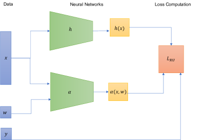
Figure 2: RU Regression architecture for policy learning. We note that the function $h$ takes $X$ as input and the auxiliary function $\alpha$ takes $X,W$ as input.

There are a few subtle differences between the RU Regression implementation in this work and that of Sahoo et al. (2022). From Theorem 8, the auxiliary function $\alpha$ in the policy learning setting depends on covariates $X$ and the treatment assignment $W$, while in the regression setting of Sahoo et al. (2022), $\alpha$ only depends on $X$. This is reflected in our architecture for learning $h,\alpha$ (Figure 2).

We note that the value functions $v_{\text{maxmin}}$ in (36) and $v_{\text{gain}}$ in (37) are unbounded above, so they do not have maximizers over unbounded function classes. To ensure that the RU loss (31) is not unbounded below when $v_{\text{maxmin}}$ or $v_{\text{gain}}$ are plugged into (31), we perform the optimization of $h$ over a class of bounded functions. In particular, we aim to learn a regression function $h_{\Gamma}(x):\mathcal{X}\rightarrow[0,1].$ Then we determine treatment assignment by computing

$$\pi_{\Gamma}(x)=\mathbb{I}\Big{(}h_{\Gamma}(x)\geq\frac{1}{2}\Big{)}.$$

Since the policy only depends on whether $h$ is greater or less than $\frac{1}{2}$, the restriction of $h$ to the class of bounded functions does not impact the optimal policy value. To enforce that $h$ must have outputs in $[0,1]$, we add a sigmoid activation as the final activation function of the neural network that represents $h$, which ensures that the network outputs values in $[0,1].$

5.2 Toy Experiment

First, we consider a simple one-dimensional experiment, so that we can visualize the data distributions and compare the learned policies to the optimal policies computed under the data model.

5.2.1 Data

Figure 3: We visualize the potential outcome distribution as $p$ varies. When $p$ is low, our potential outcome distribution mostly consists of units for which $Y_{i}(1)>Y_{i}(0)$. As $p$ increases, a larger fraction of units have $Y_{i}(0)>Y_{i}(1).$

We consider a toy example where the study and target potential outcome distribution are generated as follows. Let $U_{i}$ be an unobserved variable that impacts $Y_{i}(1).$

$$\begin{split}X_{i}&\sim\text{Uniform}[-3,3]\\ U_{i}&\sim\text{Bernoulli}(p)\\ Y_{i}(0)\mid X_{i}&\sim N(\sin(X_{i})\,,\sigma^{2})\\ Y_{i}(1)\mid X_{i}&\sim N(\sin(X_{i})+1.5-U_{i}\cdot(5X_{i})_{+}\,,\sigma^{2}),\end{split}$$ (39)

where $\sigma=0.2.$ We visualize the potential outcome distributions in Figure 3. We generate study and target potential outcome distributions by varying the Bernoulli parameter $p$ of the distribution of $U_{i}$. Let the study potential outcome distribution $P$ correspond to the potential outcome distribution where $p_{\text{study}}=0.2$. Given $P$, we generate the observed data distribution $P_{\text{obs}}$ over $(X_{i},Y_{i},W_{i})$ as follows

$$W_{i}\sim\text{Bernoulli}(0.5),\quad Y_{i}=Y_{i}(W_{i}).$$

The target potential outcome distributions $Q$ are generated by varying $p_{\text{target}}\in[0,1].$

5.2.2 Policies

We use RU Regression, with the implementation described in Section 5.1, to learn the optimal max-min and max-min gain policies with access only to data from the observed data distribution. Since this is a one-dimensional synthetic example, we also use the data model (39) and the closed-form formula (23) to compute the minimax regret policy.

We evaluate the following 4 following policies.

1. Max-Min Policy (learned via RU Regression).

2. Max-Min Gain Policy with Always Control Baseline (learned via RU Regression).

3. Max-Min Gain Policy with Always Treat Baseline (learned via RU Regression).

4. Minimax Regret (computed using (39) and (23)).

5.2.3 Results

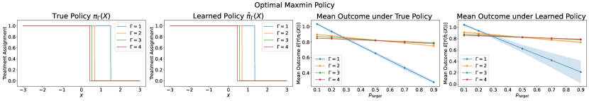
Figure 4: Max-min policy results for one-dimensional toy example. Left: We visualize the true max-min policies, computed using the data model (39). Middle Left: For one random seed, we visualize the learned maxmin policy. Middle Right: We visualize the mean outcome of the true policy for target distributions with different $p_{\text{target}}$, aggregated over 6 random trials, where the randomness is over dataset generation. Right: We visualize the mean outcome of the learned policy for target distributions with different $p_{\text{target}}$, aggregated over 6 random trials, where the randomness is over dataset generation.

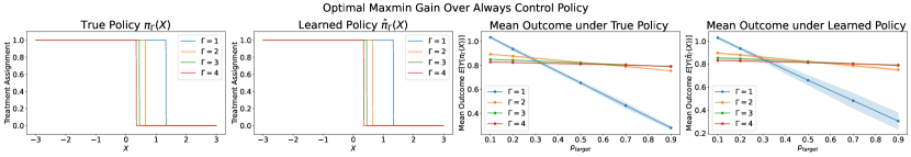
Figure 5: Max-min gain (over always control) policy results for one-dimensional toy example. Left: We visualize the true max-min gain policies where the baseline is $\pi_{0}(X)=0$ (always control), computed using the data model (39). Middle Left: For one random seed, we visualize the learned maxmin gain over always control policy. Middle Right: We visualize the mean outcome of the true policy for target distributions with different $p_{\text{target}}$, aggregated over 6 random trials, where the randomness is over dataset generation. Right: We visualize the mean outcome of the learned policy for target distributions with different $p_{\text{target}}$, aggregated over 6 random trials, where the randomness is over dataset generation.

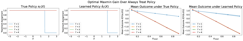
Figure 6: Max-min gain (over always treat) policy results for one-dimensional toy example. Left: We visualize the true max-min gain policies where the baseline is $\pi_{0}(X)=1$ (always treat), computed using the data model (39). Middle Left: For one random seed, we visualize the learned maxmin gain over always control policy. Middle Right: We visualize the mean outcome of the true policy for target distributions with different $p_{\text{target}}$, aggregated over 6 random trials, where the randomness is over dataset generation. Right: We visualize the mean outcome of the learned policy for target distributions with different $p_{\text{target}}$, aggregated over 6 random trials, where the randomness is over dataset generation.

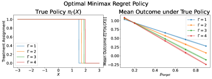
Figure 7: Minimax regret policy results for one-dimensional toy example. Left: We visualize the true minimax regret policies, computed using the data model (39). Right: We visualize the mean outcome of the learned policy for target distributions with different $p_{\text{target}}$, aggregated over 6 random trials, where the randomness is over dataset generation.

We use the data model in (39) to compute the nuisance parameters $\tau(\cdot),H_{\Gamma}(\cdot),H_{\Gamma}^{+}(\cdot),H_{\Gamma}^{-}(\cdot)$ and plug them into (17) and (21) to compute the true optimal policies. A comparison of the left and middle left plots of Figures 4, 5, 6 reveals that our learned policies match the true policies. A comparison of the middle right and right plots of Figures 4, 5, 6 demonstrates that over 6 random trials, the learned policies and the true policies achieve similar mean outcome.

Note that $\pi_{\text{non-robust}}$ from (15) is equal to the optimal max-min, max-min gain, or minimax regret policies when $\Gamma=1$. The non-robust policy recommends to treat units with nonnegative CATE. This strategy performs well when $p_{\text{target}}<0.3$ but it is outperformed by the max-min policy and the max-min gain over always control policy when $p_{\text{target}}>0.3.$ We note that the max-min gain over always treat policy does not deviate from the baseline for $\Gamma>1.$ Somewhat surprisingly, in this particular example, the minimax regret policy is less conservative that $\pi_{\text{non-robust}}$ (Figure 7) because it recommends treatment to a higher proportion of the population than $\pi_{\text{non-robust}}$ as $\Gamma$ increases.

5.3 High-Dimensional Experiment

Second, we evaluate our methods in a high-dimensional $(d=10)$ simulation.

5.3.1 Data

We consider a high-dimensional $(d=10)$ example where the study and target potential outcome distribution are generated as follows. Let $U_{i}$ be an unobserved variable that impacts $Y_{i}(1).$

$$\begin{split}X_{i}&\sim\text{Uniform}[-3,3]^{d}\\ U_{i}&\sim\text{Bernoulli}(p)\\ Y_{i}(0)\mid X_{i}&\sim N(\sin(a^{T}X_{i})\,,\sigma^{2})\\ Y_{i}(1)\mid X_{i}&\sim N(\sin(a^{T}X_{i})+1.5-U_{i}\cdot(2(X_{i,1}+X_{i,2}+X_{i,3}))_{+}\,,\sigma^{2}),\end{split}$$ (40)

where $\sigma=0.2$ and $a$ is a constant vector defined in Section B.

5.3.2 Policies

We evaluate the following policies.

1. Max-Min (learned via RU Regression)

2. Max-Min Gain over Baseline Policy (learned via RU Regression)

   $$\pi_{0}(X)=\mathbb{I}(X_{1}\leq 0).$$

5.3.3 Results

Figure 8: Max-min policy results from high-dimensional simulation.

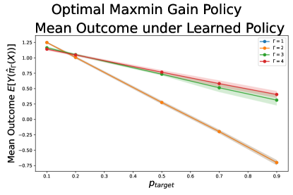
Figure 9: Max-min gain policy results from high-dimensional simulation. We note that when $\Gamma=1,2$, the max-min gain policy does not deviate from $\pi_{\text{non-robust}}$. For higher values of $\Gamma$, the max-min gain policy outperforms $\pi_{\text{non-robust}}$ for high values of $p_{\text{target}}.$

As in the toy experiments, we observe that when $\Gamma=1$ the optimal robust policies corresponds to $\pi_{\text{non-robust}}.$ As before, we observe that $\pi_{\text{non-robust}}$ performs well when $p_{\text{target}}$ is small but deteriorates in performance for larger values of $p_{\text{target}}.$ In contrast, when $\Gamma>1$, the max-min (Figure 8) and max-min gain (Figure 9) policies are more robust to changes in $p_{\text{target}}$.

5.4 Semi-Synthetic Experiment with Voting Dataset

We compare the behavior of the max-min and max-min gain policies in a semi-synthetic experiment, where we use the voting dataset of Gerber et al. (2008).

5.4.1 Data

The voting dataset of Gerber et al. (2008) was collected from a randomized controlled trial-style study that aimed to effect of various actions on voter turnout. The researchers designed one control and four treatment actions that involved mailing the selected units a letter ahead of the 2006 Michigan primary election. In the original field experiment, the probability of the control action was $\frac{5}{9}$ and the probability of each treatment action was $\frac{1}{9}.$

In our experiment we focus on only on the “Control” action $(W_{i}=0)$ and the “Neighbors” action ($W_{i}=1$). Note that this implies that the probability of treatment is $e=\frac{1}{9}/(\frac{1}{9}+\frac{5}{9})=\frac{1}{6}$. The “Neighbors” action entailed mailing a letter to the individual that contained voting participation records of the individual, the other members of the individual’s household, as well as the neighbors. The letter also mentioned a follow-up letter will be sent after the election with everyone’s updated participation, so the individual’s participation will be made known among the neighbors. The “Control” action sends no letter to the individual.

In our experiment, the covariates $X_{i}$ include the household size of the individual, age, sex, and whether the individual $i$ voted in the previous primary elections from 2000-2002 and the previous general elections from 2000-2004. The outcome $Y_{i}$ is whether individual $i$ voted in the 2006 primary election. Although the dataset also contains information on whether individual $i$ voted in the 2004 primary election, we treat this as an unobserved variable $U_{i}$ and use it generate synthetic target and study populations.

Through a dataset generation procedure described in Appendix B.3, we create a combined training and validation dataset where 67$\%$ of the units have $U_{i}=1$. In contrast, units with $U_{i}=1$ make up the only 18$\%$ of the test dataset. The training, validation, and test sets consist of 62044, 41364, and 126036 samples. By design, units who voted in the 2004 election are over-represented in the study population compared to the target population. We fit policies using data from the synthetic study population and evaluate the mean outcome under the synthetic target population.

5.4.2 Policies

We evaluate the following policies.

1. Max-Min (learned via RU Regression)

2. Max-Min Gain with Always Control Baseline (learned via RU Regression)

   $$\pi_{0}(X)=0.$$

3. Max-Min Gain with Always Treat Baseline (learned via RU Regression)

   $$\pi_{0}(X)=1.$$

5.4.3 Results

Recall that as before, $\Gamma=1$ corresponds to $\pi_{\text{non-robust}}$, so we report results for $\pi_{\text{non-robust}}$ (learned via RU Regression with $v_{\text{maxmin}}$ and $\Gamma=1$). We evaluate the robust policies learned for $\Gamma=1.1,1.2,1.3,1.5,2,3,4$. We simply report results for $\Gamma=1.1,1.2,1.3,1.5$ because when $\Gamma\geq 1.5$ we observe the same results as when $\Gamma=1.5$. This can be explained by the fact that the outcomes $Y_{i}(0),Y_{i}(1)$ are binary-valued, so $q_{\zeta(\Gamma)}(Y(w)\mid X=x)$ may take on the same value for many values of $\Gamma$. Note that our theoretical results only apply to the case where the conditional study potential outcome distribution is absolutely continuous with respect to Lebesgue measure, but in this experiment, the study potential outcome distribution is a discrete distribution. Nevertheless, we observe results that are in line with our results for continuous-valued outcomes. We report the target policy value and the proportion of target population treated under the different learned policies in Table 1. We find that the non-robust policy recommends recommends to treat about 66% of the population. We find that the max-min and max-min gain over always treat baseline policy recommends to treat the entire population. In contrast, the max-min gain over the always control baseline recommends to treat a decreasing fraction of the population as $\Gamma$ increases. In this particular example, we observe that different robust objective functions can yield very different policies.

Method	Target Policy Value	Proportion of Target Population Treated
Non-Robust	0.3106 $\pm$ 0.003	0.66
Max-Min $(\Gamma=1.1)$	0.3272 $\pm$ 0.003	0.87
Max-Min $(\Gamma=1.2)$	0.3375 $\pm$ 0.004	1.0
Max-Min $(\Gamma=1.3)$	0.3375 $\pm$ 0.004	1.0
Max-Min $(\Gamma=1.5)$	0.3375 $\pm$ 0.004	1.0
Max-Min Gain over Always Treat $(\Gamma=1.1)$	0.3375 $\pm$ 0.004	1.0
Max-Min Gain over Always Treat $(\Gamma=1.2)$	0.3375 $\pm$ 0.004	1.0
Max-Min Gain over Always Treat $(\Gamma=1.3)$	0.3375 $\pm$ 0.004	1.0
Max-Min Gain over Always Treat $(\Gamma=1.5)$	0.3375 $\pm$ 0.004	1.0
Max-Min Gain over Always Control $(\Gamma=1.1)$	0.2934 $\pm$ 0.003	0.44
Max-Min Gain over Always Control $(\Gamma=1.2)$	0.2780 $\pm$ 0.002	0.25
Max-Min Gain over Always Control $(\Gamma=1.3)$	0.2705 $\pm$ 0.002	0.15
Max-Min Gain over Always Control $(\Gamma=1.5)$	0.2653 $\pm$ 0.001	0.0

Table 1: The non-robust policy recommends to treat 66% of the population. The max-min and max-min gain over always treat policies recommend to treat the entire population. In contrast, the max-min gain over always control policies recommends treatment to a much smaller proportion of the population.

Appendix A Additional Experimental Results

Method	Target Policy Value
	$p=0.1$	$p=0.2$	$p=0.5$	$p=0.7$	$p=0.9$
RU Regression	1.029 $\pm$ 0.016	0.930 $\pm$ 0.009	0.659 $\pm$ 0.015	0.491 $\pm$ 0.025	0.308 $\pm$ 0.062
$(\Gamma=1)$
True	1.035 $\pm$ 0.010	0.937 $\pm$ 0.016	0.654 $\pm$ 0.015	0.464 $\pm$ 0.025	0.278 $\pm$ 0.015
$(\Gamma=1)$
RU Regression	0.908 $\pm$ 0.015	0.882 $\pm$ 0.007	0.819 $\pm$ 0.003	0.780 $\pm$ 0.017	0.740 $\pm$ 0.019
$(\Gamma=2)$
True	0.899 $\pm$ 0.005	0.881 $\pm$ 0.007	0.824 $\pm$ 0.005	0.787 $\pm$ 0.006	0.749 $\pm$ 0.004
$(\Gamma=2)$
RU Regression	0.874 $\pm$ 0.008	0.861 $\pm$ 0.009	0.823 $\pm$ 0.003	0.801 $\pm$ 0.002	0.776 $\pm$ 0.009
$(\Gamma=3)$
True	0.873 $\pm$ 0.003	0.863 $\pm$ 0.005	0.824 $\pm$ 0.005	0.802 $\pm$ 0.004	0.778 $\pm$ 0.003
$(\Gamma=3)$
RU Regression	0.856 $\pm$ 0.010	0.847 $\pm$ 0.009	0.819 $\pm$ 0.001	0.804 $\pm$ 0.004	0.785 $\pm$ 0.008
$(\Gamma=4)$
True	0.850 $\pm$ 0.004	0.844 $\pm$ 0.006	0.820 $\pm$ 0.005	0.806 $\pm$ 0.004	0.790 $\pm$ 0.003
$(\Gamma=4)$

Table 2: Max-min policy results from one-dimensional simulation experiment. We report the mean and standard deviation of the target policy value from 6 random trials, where the randomness is over the dataset generation. Note that RU Regression with $\Gamma=1$ yields a policy that is equivalent to $\pi_{\text{non-robust}}$ and incurs low policy value for low values of $p$. The maxmin policies $\hat{\pi}_{\Gamma}$ for $\Gamma>1$ yield higher policy values for high values of $p$.

Method	Target Policy Value
	$p=0.1$	$p=0.2$	$p=0.5$	$p=0.7$	$p=0.9$
RU Regression	1.031 $\pm$ 0.016	0.930 $\pm$ 0.010	0.656 $\pm$ 0.019	0.484 $\pm$ 0.024	0.301 $\pm$ 0.057
$(\Gamma=1)$
True	1.035 $\pm$ 0.010	0.937 $\pm$ 0.016	0.654 $\pm$ 0.015	0.464 $\pm$ 0.025	0.278 $\pm$ 0.015
$(\Gamma=1)$
RU Regression	0.897 $\pm$ 0.011	0.876 $\pm$ 0.005	0.821 $\pm$ 0.003	0.788 $\pm$ 0.010	0.753 $\pm$ 0.011
$(\Gamma=2)$
True	0.894 $\pm$ 0.004	0.878 $\pm$ 0.006	0.825 $\pm$ 0.005	0.791 $\pm$ 0.005	0.755 $\pm$ 0.003
$(\Gamma=2)$
RU Regression	0.854 $\pm$ 0.009	0.846 $\pm$ 0.008	0.818 $\pm$ 0.002	0.804 $\pm$ 0.004	0.788 $\pm$ 0.008
$(\Gamma=3)$
True	0.850 $\pm$ 0.004	0.844 $\pm$ 0.006	0.820 $\pm$ 0.005	0.806 $\pm$ 0.004	0.790 $\pm$ 0.003
$(\Gamma=3)$
RU Regression	0.834 $\pm$ 0.006	0.827 $\pm$ 0.005	0.812 $\pm$ 0.001	0.801 $\pm$ 0.005	0.792 $\pm$ 0.004
$(\Gamma=4)$
True	0.829 $\pm$ 0.005	0.824 $\pm$ 0.005	0.811 $\pm$ 0.004	0.802 $\pm$ 0.004	0.793 $\pm$ 0.003
$(\Gamma=4)$

Table 3: Max-min gain over always control policy results from one-dimensional simulation experiment. We report the mean and standard deviation of the target policy value from 6 random trials, where the randomness is over the dataset generation. Note that RU Regression with $\Gamma=1$ yields a policy that is equivalent to $\pi_{\text{non-robust}}$ and incurs low policy value for low values of $p$. The maxmin gain over always control policies $\hat{\pi}_{\Gamma}$ for $\Gamma>1$ yield higher policy values for high values of $p$.

Method	Target Policy Value
	$p=0.1$	$p=0.2$	$p=0.5$	$p=0.7$	$p=0.9$
RU Regression	1.028 $\pm$ 0.016	0.929 $\pm$ 0.009	0.660 $\pm$ 0.020	0.492 $\pm$ 0.029	0.311 $\pm$ 0.066
$(\Gamma=1)$
True	1.035 $\pm$ 0.010	0.937 $\pm$ 0.016	0.654 $\pm$ 0.015	0.464 $\pm$ 0.025	0.278 $\pm$ 0.015
$(\Gamma=1)$
RU Regression	1.124 $\pm$ 0.021	0.755 $\pm$ 0.019	-0.355 $\pm$ 0.035	-1.131 $\pm$ 0.043	-1.856 $\pm$ 0.032
$(\Gamma=2)$
True	1.126 $\pm$ 0.022	0.760 $\pm$ 0.019	-0.358 $\pm$ 0.031	-1.139 $\pm$ 0.037	-1.875 $\pm$ 0.039
$(\Gamma=2)$
RU Regression	1.124 $\pm$ 0.021	0.755 $\pm$ 0.019	-0.355 $\pm$ 0.035	-1.131 $\pm$ 0.043	-1.856 $\pm$ 0.032
$(\Gamma=3)$
True	1.126 $\pm$ 0.022	0.760 $\pm$ 0.019	-0.358 $\pm$ 0.031	-1.139 $\pm$ 0.037	-1.875 $\pm$ 0.039
$(\Gamma=3)$
RU Regression	1.121 $\pm$ 0.025	0.747 $\pm$ 0.013	-0.356 $\pm$ 0.043	-1.127 $\pm$ 0.052	-1.841 $\pm$ 0.012
$(\Gamma=4)$
True	1.126 $\pm$ 0.022	0.760 $\pm$ 0.019	-0.358 $\pm$ 0.031	-1.139 $\pm$ 0.037	-1.875 $\pm$ 0.039
$(\Gamma=4)$

Table 4: Max-min gain over always treat policy results from one-dimensional simulation experiment. We report the mean and standard deviation of the target policy value from 6 random trials, where the randomness is over the dataset generation. Note that RU Regression with $\Gamma=1$ yields a policy that is equivalent to $\pi_{\text{non-robust}}$. This max-min gain policy defaults to the baseline policy $\pi_{0}(x)=1$ for $\Gamma>1$.

Method	Target Policy Value
	$p=0.1$	$p=0.2$	$p=0.5$	$p=0.7$	$p=0.9$
RU Regression	1.249 $\pm$ 0.012	1.007 $\pm$ 0.019	0.275 $\pm$ 0.027	-0.198 $\pm$ 0.030	-0.701 $\pm$ 0.042
$(\Gamma=1)$
RU Regression	1.249 $\pm$ 0.012	1.007 $\pm$ 0.019	0.275 $\pm$ 0.027	-0.198 $\pm$ 0.030	-0.701 $\pm$ 0.042
$(\Gamma=2)$
RU Regression	1.164 $\pm$ 0.020	1.052 $\pm$ 0.018	0.734 $\pm$ 0.021	0.514 $\pm$ 0.069	0.313 $\pm$ 0.086
$(\Gamma=3)$
RU Regression	1.141 $\pm$ 0.023	1.047 $\pm$ 0.018	0.767 $\pm$ 0.033	0.581 $\pm$ 0.052	0.405 $\pm$ 0.055
$(\Gamma=4)$

Table 5: Max-min gain policy results for high-dimensional simulation.

Method	Target Policy Value
	$p=0.1$	$p=0.2$	$p=0.5$	$p=0.7$	$p=0.9$
RU Regression	1.249 $\pm$ 0.012	1.007 $\pm$ 0.019	0.275 $\pm$ 0.027	-0.198 $\pm$ 0.030	-0.701 $\pm$ 0.042
$(\Gamma=1)$
RU Regression	1.099 $\pm$ 0.021	1.030 $\pm$ 0.016	0.828 $\pm$ 0.021	0.690 $\pm$ 0.030	0.563 $\pm$ 0.033
$(\Gamma=2)$
RU Regression	1.061 $\pm$ 0.020	1.008 $\pm$ 0.022	0.850 $\pm$ 0.020	0.741 $\pm$ 0.025	0.643 $\pm$ 0.028
$(\Gamma=3)$
RU Regression	1.018 $\pm$ 0.019	0.977 $\pm$ 0.024	0.868 $\pm$ 0.017	0.791 $\pm$ 0.014	0.724 $\pm$ 0.022
$(\Gamma=4)$

Table 6: Max-min gain policy results for high-dimensional simulation.

Appendix B Experimental Details

B.1 Toy Example

B.1.1 Model

For the RU Regression model, we jointly train two neural networks to learn the regression function $h$ and the quantile function $\alpha$, respectively. A visualization of the model architecture for RU Regression is provided in Figure 2. Each of the neural networks has 3 hidden layers and 64 units per layer and ReLU activation. The RU Regression model has 17.1K trainable parameters.

B.1.2 Dataset Splits

For all methods, the train, validation, and test sets consists of 20000, 10000, and 10000 samples, respectively. The train and validation sets are generated via the data model specified in (39) with $p=0.2.$ All methods are evaluated on the same test sets, which are generated via the data model in (39) parameter $p$ taking value in $[0.1,0.2,0.5,0.7,0.9]$. For each of 6 random seeds $[0,1,2,3,4,5]$, a new dataset (train, validation, test set) is generated.

B.1.3 Training Procedure

The models are trained for a maximum of $50$ epochs with batch size equal to $4000$ and we use the Adam optimizer with learning rate $1e-2$. Each epoch we check the loss obtained on the validation set and select the model that minimizes the loss on the validation set.

B.2 High-Dimensional Experiment

B.2.1 Data

In the data model from (40), we set

$$a= [0.50067509,-0.67108696,-2.22006362,-0.37834265,1.05841302,$$

$$-0.4509034,1.15857361,0.62236239,-0.77458079,-0.74790281].$$

B.2.2 Model

We use the same models as in toy experiment (See Section B.1.1).

B.2.3 Dataset Splits

We use the same dataset splits as in the toy experiment (See Section B.1.2)

B.2.4 Training Procedure

We use the same training procedure as in the toy experiment(See Section B.1.3).

B.3 Voting Semi-Synthetic Experiment

B.3.1 Model

We use the same models as in toy experiment (See Section B.1.1).

B.3.2 Dataset Splits

We randomly select 75$\%$ of units with $U_{i}=1$ and 25$\%$ of units with $U_{i}=0$ to create the combined training and validation dataset, which represents the study population. The remaining units make up the test set, which represents the target population.

B.3.3 Training Procedure

We use the same training procedure as in the toy experiment(See Section B.1.3).

Appendix C Standard Results

Lemma 14.

Let $\zeta\in(0,1).$ CVaR has the following properties:

1. If $Y$ has a density, then

   $$\mathbb{E}\left[Y\right]=(1-\zeta)\mathrm{CVaR}_{\zeta}(Y)-\zeta\mathrm{CVaR}_{1-\zeta}(-Y),$$

2. $\mathrm{CVaR}$ is positively homogenenous, i.e.

   $$\mathrm{CVaR}_{\zeta}(cY)=c\mathrm{CVaR}_{\zeta}(Y)$$

   if $c>0,$

[Pflug, 2000].

Lemma 15.

For probability measures with finite second moment, CVaR is a strongly coherent risk measure, meaning it is convex, continuous, and for random variables $X,Y$ with absolutely continuous distributions $F_{X},F_{Y}$

$$\mathrm{CVaR}(X)+\mathrm{CVaR}(Y)=\sup\{\mathrm{CVaR}(\tilde{X}+\tilde{Y}):(\tilde{X},\tilde{Y})\sim\mu,\mu\in\mathcal{T}(F_{X},F_{Y})\}$$

where $\mathcal{T}$ is the set of all bivariate distributions with marginals $F_{X},F_{Y}$ [Ekeland et al., 2012].

Proposition 16.

Let $f$ be a convex function, and let $C$ be a closed bounded convex set contained in $\mathrm{dom}f$. Then the supremum of $f$ relative to $C$ is finite and it is attained at some extreme point of $C$ [Rockafellar, 1997].

Lemma 17.

Let $J(z)=A\log(1+\exp\{2z-1\})+B\log(1+\exp\{-2z+1\}).$ Let $z^{*}=\operatorname*{argmax}_{z\in[0,1]}J(z)$. $A\geq B$ iff $z^{*}\geq\frac{1}{2}.$ Proof in Appendix E.1.

Appendix D Proofs of Main Results

D.1 Notation

We use the following notation in the proofs. Here, we assume that $Y(0),Y(1)$ are distributed according to a potential outcome distribution whose marginals match those of $P_{\text{obs}}$

$$c_{1}^{+}(x) =\text{CVaR}_{\zeta(\Gamma)}(Y(1)\mid x)$$

$$c_{1}^{-}(x) =\text{CVaR}_{\zeta(\Gamma)}(-Y(1)\mid x)$$

$$c_{0}^{+}(x) =\text{CVaR}_{\zeta(\Gamma)}(Y(0)\mid x)$$

$$c_{0}^{-}(x) =\text{CVaR}_{\zeta(\Gamma)}(-Y(0)\mid x)$$

$$g_{1}(x) =\Gamma\tau(x)+(1-\Gamma)(c_{1}^{+}(x)+c_{0}^{-}(x))$$

$$g_{0}(x) =-\Gamma\tau(x)+(1-\Gamma)(c_{0}^{+}(x)+c_{1}^{-}(x)).$$

Note that

$$H_{\Gamma}^{+}(x) =(1-\Gamma^{-1})\cdot(c_{1}^{+}(x)+c_{0}^{-}(x))$$

$$H_{\Gamma}^{-}(x) =(1-\Gamma^{-1})\cdot(-c_{1}^{-}(x)-c_{0}^{+}(x))$$

$$\tau(x)\geq H_{\Gamma}^{+}(x) \Longleftrightarrow g_{1}(x)\geq 0$$

$$\tau(x)\geq H_{\Gamma}^{-}(x) \Longleftrightarrow g_{0}(x)\leq 0.$$

Throughout this section, we assume that $P_{(Y(1),Y(0))\mid X=x}$ is absolutely continuous with respect to Lebesgue measure almost surely for any $x$.

D.2 Technical Lemmas

Lemma 18.

Let $P,Q$ be potential outcome distributions. $Q$ generates $P$ via $\Gamma$-biased sampling if and only if

$$\Gamma^{-1}\leq\frac{dQ_{Y(0),Y(1)\mid X=x}(y_{0},y_{1})}{dP_{Y(0),Y(1)\mid X=x}(y_{0},y_{1})}\leq\Gamma\quad\forall x\in\mathcal{X},y_{0},y_{1}\in\mathbb{R}$$ (41)

and $\sup_{x\in\mathcal{X}}\frac{dP_{X}(x)}{dQ_{X}(x)}<\infty.$ Proof in Appendix E.8.

Lemma 19.

A policy $\pi$ solves (26) for every $Q_{X}$ such that $Q_{X}\ll P_{\mathrm{obs},X}$ and $\sup_{x\in\mathcal{X}}\frac{dP_{\mathrm{obs},X}(x)}{dQ_{X}(x)}<\infty$ iff $\pi$ solves

$$\max_{\pi(x)\in\{0,1\}}\inf_{P\in\mathcal{T}(P_{\mathrm{obs}})}\Gamma\mathbb{E}_{P}\left[v^{*}(\pi(x);X,Y(0),Y(1))\mid X=x\right]+(1-\Gamma)\mathrm{CVaR}_{\zeta(\Gamma)}(v^{*}(\pi(x);X,Y(0),Y(1))\mid x)$$ (42)

for every $x\in\mathrm{supp}(P_{\mathrm{obs},X}).$ Similarly, a function $h$ solves (30) for every $Q_{X}$ such that $Q_{X}\ll P_{\mathrm{obs},X}$ and $\sup_{x\in\mathcal{X}}\frac{dP_{\mathrm{obs},X}(x)}{dQ_{X}(x)}<\infty$ if and only if it solves

$$\max_{h(x)\in[0,1]}\inf_{P\in\mathcal{T}(P_{\mathrm{obs}})}\Gamma\mathbb{E}_{P}\left[v^{*}(h(x);X,Y(0),Y(1))\mid X=x\right]+(1-\Gamma)\mathrm{CVaR}_{\zeta(\Gamma)}(v^{*}(h(x);X,Y(0),Y(1))\mid x)$$ (43)

for every $x\in\mathrm{supp}(P_{\mathrm{obs},X}).$ Proof in Appendix E.3.

Lemma 20.

Let $v^{*}(z;x,y_{0},y_{1})=(z-\pi_{0}(x))\cdot(y_{1}-y_{0}).$ Suppose that $Q_{X}$ satisfies $Q_{X}\ll P_{\mathrm{obs},X}$ and $\sup_{x\in\mathcal{X}}\frac{dP_{\mathrm{obs},X}(x)}{dQ_{X}(x)}<\infty.$ Then,

$$\inf_{Q\in\mathcal{S}^{\Gamma}(P_{\mathrm{obs}},Q_{X})}\mathbb{E}_{Q}\left[v^{*}(\pi(X);X,Y(0),Y(1))\mid X=x\right]$$ (44)

$$=(\pi(x)-\pi_{0}(x))_{+}g_{1}(x)+(\pi_{0}(x)-\pi(x))_{+}g_{0}(x),$$

for any $x\in\mathrm{supp}(P_{\mathrm{obs},X}).$ Proof in Appendix E.4.

Lemma 21.

For $x\in\mathrm{supp}(P_{\mathrm{obs},X})$, $\min\{g_{1}(x),g_{0}(x)\}\leq 0.$ In addition, if $g_{1}(x)=0$, then $g_{0}(x)\leq 0.$ Proof in Appendix E.5.

Lemma 22.

Let $P_{\mathrm{obs}}$ be an observed data distribution where $P_{\mathrm{obs},W\mid X}=\mathrm{Bernoulli}(e)$ for a treatment probability $e$. Let $Q\in\mathcal{S}^{\Gamma}(P_{\mathrm{obs}},Q_{X})$. Suppose that under an RCT with treatment probability $e$, the potential outcome distribution $Q$ yields the observed data distribution $Q_{\mathrm{obs}}.$ Then, $Q_{\mathrm{obs}}\in\mathcal{S}^{\Gamma}_{\mathrm{obs}}(P_{\mathrm{obs}},Q_{X}).$ Proof in Appendix E.6.

Lemma 23.

Let $\zeta(\Gamma)=\frac{1}{\Gamma+1}.$ Let $q_{\zeta}(v(h(x);X,Y,W)\mid x,w)$ be the $\zeta$-th quantile of $v(h(x);x,Y,w)$ where $Y\sim P_{\mathrm{obs},Y\mid X=x,W=w}.$ The distribution $dQ^{*}_{\mathrm{obs}}$ that solves

$$\operatorname*{argmin}_{Q_{\mathrm{obs}}\in\mathcal{S}^{\Gamma}_{\mathrm{obs}}(P_{\mathrm{obs}},Q_{X})}\mathbb{E}_{Q_{\mathrm{obs}}}\left[v(h(x);X,Y,W)\right]$$ (45)

is given by $dQ_{X}\cdot dP_{\mathrm{obs},W\mid X}\cdot dQ^{*}_{\mathrm{obs},Y\mid X,W}$, where

$$dQ_{\mathrm{obs},Y\mid X=x,W=w}^{*}(y)=\begin{cases}\Gamma^{-1}\cdot dP_{\mathrm{obs},Y\mid X=x,W=w}(y)&v(h(x);x,y,w)\geq q_{\zeta(\Gamma)}(v(h(x);X,Y,W)\mid w,x)\\ \Gamma\cdot dP_{\mathrm{obs},Y\mid X=x,W=w}(y)&\mathrm{o.w.}.\end{cases}$$ (46)

Proof in Appendix E.7.

Lemma 24.

Let $P,Q$ be potential outcome distributions. If $Q$ generates $P$ via $\Gamma$-biased sampling, then

$$\Gamma^{-1}\leq\frac{dQ_{Y(w)\mid X=x}(y)}{dP_{Y(w)\mid X=x}(y)}\leq\Gamma\quad\forall x\in\mathcal{X},y\in\mathbb{R},w\in\{0,1\}$$ (47)

and $\sup_{x\in\mathcal{X}}\frac{dP_{\mathrm{obs},X}(x)}{dQ_{X}(x)}<\infty$. Proof in Appendix E.8.

D.3 Proof of Theorem 1

Define $v^{*}(\pi(X);X,Y(0),Y(1))=Y(\pi(X))=\pi(X)\cdot Y(1)+(1-\pi(X))Y(0).$ We can apply Lemma 19 to see that solving (10) for any $Q_{X}$ such that $Q_{X}\ll P_{\text{obs},X}$ and $\sup_{x\in\mathcal{X}}\frac{dP_{\text{obs},X}(x)}{dQ_{X}(x)}<\infty$ is equivalent to solving the following conditional worst-case risk minimization problem

$$\max_{\pi(x)\in\{0,1\}}\inf_{P\in\mathcal{T}(P_{\text{obs}})}\Gamma\mathbb{E}_{P}\left[Y(\pi(x))\mid X=x\right]+(1-\Gamma)\text{CVaR}_{\zeta(\Gamma)}(Y(\pi(x))\mid x)$$ (48)

for every $x\in\text{supp}(P_{\text{obs},X})$.

We note that

$$\mathbb{E}_{P}\left[Y(\pi(x))\mid X=x\right]=\pi(x)\mathbb{E}_{P}\left[Y(1)\mid X=x\right]+(1-\pi(x))\mathbb{E}_{P}\left[Y(0)\mid X=x\right],$$

so this term is identified under $P_{\text{obs}}$ and does not depend on the choice of $P\in\mathcal{T}(P_{\text{obs}}).$ Let $P$ be any potential outcome distribution $\mathcal{T}(P_{\text{obs}}).$ So, (48) can be written as

$$\max_{\pi(x)\in\{0,1\}}\Gamma(\pi(x)\mathbb{E}_{P}\left[Y(1)\mid X=x\right]+(1-\pi(x))\mathbb{E}_{P}\left[Y(1)\mid X=x\right])+\inf_{P^{\prime}\in\mathcal{T}(P_{\text{obs}})}(1-\Gamma)\text{CVaR}_{\zeta(\Gamma)}(Y(\pi(x))\mid x).$$ (49)

Simplifying the term on the right, we have that

$$\inf_{P^{\prime}\in\mathcal{T}(P_{\text{obs}})}(1-\Gamma)\text{CVaR}_{\zeta(\Gamma)}(Y(\pi(x))\mid x)$$ (50)

$$=(1-\Gamma)\sup_{P^{\prime}\in\mathcal{T}(P_{\text{obs}})}\text{CVaR}_{\zeta(\Gamma)}(Y(\pi(x))\mid x)$$ (51)

$$=(1-\Gamma)\sup_{P^{\prime}\in\mathcal{T}(P_{\text{obs}})}\text{CVaR}_{\zeta(\Gamma)}(\pi(x)Y(1)+(1-\pi(x))Y(0)\mid x)$$ (52)

$$=(1-\Gamma)\Big{(}\text{CVaR}_{\zeta(\Gamma)}(\pi(x)Y(1))+\text{CVaR}_{\zeta(\Gamma)}((1-\pi(x))Y(0))\Big{)}$$ (53)

$$=(1-\Gamma)\Big{(}\pi(x)\text{CVaR}_{\zeta(\Gamma)}(Y(1)\mid x)+(1-\pi(x))\text{CVaR}_{\zeta(\Gamma)}(Y(0)\mid x)\Big{)}$$ (54)

$$=(1-\Gamma)\Big{(}\pi(x)c_{1}^{+}(x)+(1-\pi(x))c_{0}^{+}(x)\Big{)}.$$ (55)

(53) follows from Lemma 15. (54) follows from Lemma 14.

Plugging in the above expression into (49) yields

$$\max_{\pi(x)\in\{0,1\}}\pi(x)(\Gamma\mathbb{E}_{P}\left[Y(1)\mid X=x\right]+(1-\Gamma)c_{1}^{+}(x))+(1-\pi(x))(\Gamma\mathbb{E}_{P}\left[Y(0)\mid X=x\right]+(1-\Gamma)c_{0}^{+}(x)).$$ (56)

Given the form of the worst-case risk above, the optimal policy is equal to

$$\mathbb{I}(\Gamma\mathbb{E}_{P}\left[Y(1)\mid X=x\right]+(1-\Gamma)c_{1}^{+}(x)\geq\Gamma\mathbb{E}_{P}\left[Y(0)\mid X=x\right]+(1-\Gamma)c_{0}^{+}(x)).$$

Rearranging terms, we have that this policy is equal to

$$\mathbb{I}(\tau(x)\geq(1-\Gamma^{-1})(c_{1}^{+}(x)-c_{0}^{+}(x))).$$

Note that this is equal to (17).

D.4 Proof of Lemma 2

We have that

$$\inf_{Q\in\mathcal{S}^{\Gamma}(P_{\text{obs}},Q_{X})}\mathbb{E}_{Q}\left[Y(w)\mid X=x\right] =\inf_{P\in\mathcal{T}(P_{\text{obs}})}\inf_{Q\in\mathcal{R}^{\Gamma}(P,Q_{X})}\mathbb{E}_{Q}\left[Y(w)\mid X=x\right]$$ (57)

$$=\inf_{P\in\mathcal{T}(P_{\text{obs}})}\Gamma\mathbb{E}_{P}\left[Y(w)\mid X=x\right]+(1-\Gamma)\text{CVaR}_{\zeta(\Gamma)}(Y(1)\mid X=x)$$ (58)

$$=\Gamma\mathbb{E}_{P}\left[Y(w)\mid X=x\right]+(1-\Gamma)c_{w}^{+}(x),$$ (59)

where $P$ is any study potential outcome distribution in $\mathcal{T}(P_{\text{obs}}).$ In the above derivation, (58) follows from Lemma 19 and (59) follows from Lemma 15. We examine the policy from (18) and find that it can be written as follows

$$\mathbb{I}\left(\inf_{Q\in\mathcal{S}^{\Gamma}(P_{\text{obs}},Q_{X})}\mathbb{E}_{Q}\left[Y(1)\mid X=x\right]\geq\inf_{Q\in\mathcal{S}^{\Gamma}(P_{\text{obs}},Q_{X})}\mathbb{E}_{Q}\left[Y(0)\mid X=x\right])\right)$$

$$=\mathbb{I}\left(\Gamma\mathbb{E}_{P}\left[Y(1)\mid X=x\right]+(1-\Gamma)c_{1}^{+}(x)\geq\Gamma\mathbb{E}_{P}\left[Y(0)\mid X=x\right]+(1-\Gamma)c_{0}^{+}(x)\right)$$

$$=\mathbb{I}(\Gamma\tau(x)\geq(\Gamma-1)(c_{1}^{+}(x)-c_{0}^{+}(x)))$$

$$=\mathbb{I}(\tau(x)\geq(1-\Gamma^{-1})(c_{1}^{+}(x)-c_{0}^{+}(x)))$$

$$=\mathbb{I}(\tau(x)\geq H_{\Gamma}(x))$$

$$=\pi_{\Gamma,\text{maxmin}}^{*}(x).$$

Thus, we conclude that the policy that compares the lower bounds on $\mathbb{E}_{Q}\left[Y(1)\mid X=x\right]$ and $\mathbb{E}_{Q}\left[Y(0)\mid X=x\right]$ over the robustness set $\mathcal{S}^{\Gamma}(P_{\text{obs}},Q_{X})$ is the max-min policy $\pi_{\Gamma,\text{maxmin}}^{*}.$

D.5 Proof of Theorem 3

We note that $\mathbb{E}_{Q}\left[Y(\pi(X))\right]-\mathbb{E}_{Q}\left[Y(\pi_{0}(X))\right]=\mathbb{E}_{Q}\left[(\pi(X)-\pi_{0}(X))\cdot(Y(1)-Y(0))\right]$, so (11) is equivalent to

$$\sup_{\pi\in\Pi}\inf_{Q\in\mathcal{S}^{\Gamma}(P_{\text{obs}},Q_{X})}\mathbb{E}_{Q}\left[v^{*}(\pi(X);X,Y(0),Y(1))\right]$$

for $v^{*}(z;x,y_{0},y_{1})=(z-\pi_{0}(x))\cdot(y_{1}-y_{0}).$ Solving the above problem for every $Q_{X}$ such that $Q_{X}\ll P_{\text{obs},X}$ and $\sup_{x\in\mathcal{X}}\frac{dP_{\text{obs},X}(x)}{dQ_{X}(x)}<\infty$ is equivalent to solving the conditional worst-case gain problem (left side of (44)) for every $x\in\text{supp}(P_{\text{obs},X}).$ Thus, we can apply Lemma 20 to see that a policy $\pi$ that solves (11) solves the right side of (44) for every $x$ in $\text{supp}(P_{\text{obs},X}).$

First, we consider the case where $\pi_{0}(x)=0.$ In this case, (44) reduces to

$$\max_{\pi(x)\in\{0,1\}}(\pi(x))_{+}(\Gamma\tau(x)+(1-\Gamma)(c_{1}^{+}(x)+c_{0}^{-}(x))).$$

So, the optimal policy when $\pi_{0}(x)=0$ is equivalent to $\mathbb{I}(\Gamma\tau(x)+(1-\Gamma)(c_{1}^{+}(x)+c_{0}^{-}(x))\geq 0).$ Rearranging terms, this is equivalent to $\mathbb{I}(\tau(x)\geq H_{\Gamma}^{+}(x)).$

Second, we consider the case where $\pi_{0}(x)=1.$ In this case, (44) reduces to

$$\max_{\pi(x)\in\{0,1\}}(1-\pi(x))_{+}(-\Gamma\tau(x)+(1-\Gamma)(c_{0}^{+}(x)+c_{1}^{-}(x))).$$

So, the optimal policy when $\pi_{0}(x)=1$ is equivalent to $\mathbb{I}(-\Gamma\tau(x)+(1-\Gamma)(c_{0}^{+}(x)+c_{1}^{-}(x))\leq 0)$. Rearranging terms, this is equivalent to $\mathbb{I}(\tau(x)\geq H_{\Gamma}^{-}(x)).$

Combining these two results yields the policy in (21).

D.6 Proof of Lemma 4

Let $q_{\zeta}(Z)$ denote the $\zeta$-th quantile of a random variable $Z$. We note that for a random variable $Z$, $q_{\zeta}(Z)=-q_{1-\zeta}(-Z).$

We note that

$$-c_{1}^{-}(x) =-\mathbb{E}_{P}\left[-Y(1)\mid-Y(1)\geq q_{\zeta(\Gamma)}(-Y(1)\mid x),X=x\right]$$

$$=\mathbb{E}_{P}\left[Y(1)\mid Y(1)\leq-q_{\zeta(\Gamma)}(-Y(1)\mid x),X=x\right]$$

$$=\mathbb{E}_{P}\left[Y(1)\mid Y(1)\leq q_{1-\zeta(\Gamma)}(Y(1)\mid x),X=x\right]$$

$$\leq\mathbb{E}_{P}\left[Y(1)\mid Y(1)\geq q_{\zeta(\Gamma)}(Y(1)\mid x),X=x\right]$$

$$=c_{1}^{+}(x).$$

This implies that

$$H^{-}_{\Gamma}(x) =(1-\Gamma^{-1})\cdot(-c_{1}^{-}(x)-c_{0}^{+}(x))$$

$$\leq(1-\Gamma^{-1})\cdot(c_{1}^{+}(x)-c_{0}^{+}(x))$$

$$=H_{\Gamma}(x).$$

Also, we have that

$$-c_{0}^{+}(x) =-\mathbb{E}_{P}\left[Y(0)\mid Y(0)\geq q_{\zeta(\Gamma)}(Y(0)\mid x),X=x\right]$$

$$=\mathbb{E}_{P}\left[-Y(0)\mid-Y(0)\leq-q_{\zeta(\Gamma)}(Y(0)\mid x),X=x\right]$$

$$=\mathbb{E}_{P}\left[-Y(0)\mid-Y(0)\leq q_{1-\zeta(\Gamma)}(-Y(0)\mid x),X=x\right]$$

$$\leq\mathbb{E}_{P}\left[-Y(0)\mid-Y(0)\geq q_{\zeta(\Gamma)}(-Y(0)\mid x),X=x\right]$$

$$=c_{0}^{-}(x).$$

This implies that

$$H_{\Gamma}(x) =(1-\Gamma^{-1})(c_{1}^{+}(x)-c_{0}^{+}(x))$$

$$\leq(1-\Gamma^{-1})(c_{1}^{+}(x)+c_{0}^{-}(x))$$

$$=H^{+}_{\Gamma}(x).$$

Combining these two results yields that $H^{-}_{\Gamma}(x)\leq H_{\Gamma}(x)\leq H^{+}_{\Gamma}(x).$

D.7 Proof of Theorem 5

We note that (12) can be expressed as follows.

$$\inf_{\pi\in\Pi}\sup_{Q\in\mathcal{S}^{\Gamma}(P_{\text{obs}},Q_{X})}R_{Q}(\pi(X)) =\inf_{\pi\in\Pi}\sup_{Q\in\mathcal{S}^{\Gamma}(P_{\text{obs}},Q_{X})}\sup_{\pi^{\prime}}\mathbb{E}_{Q}\left[Y(\pi^{\prime}(X))\right]-\mathbb{E}_{Q}\left[Y(\pi(X))\right]$$

$$=\sup_{\pi\in\Pi}\inf_{Q\in\mathcal{S}^{\Gamma}(P_{\text{obs}},Q_{X})}\mathbb{E}_{Q}\left[Y(\pi(X))\right]-\inf_{\pi^{\prime}\in\Pi}\mathbb{E}_{Q}\left[Y(\pi^{\prime}(X))\right]$$

$$=\sup_{\pi\in\Pi}\inf_{Q\in\mathcal{S}^{\Gamma}(P_{\text{obs}},Q_{X})}\inf_{\pi^{\prime}\in\Pi}\mathbb{E}_{Q}\left[Y(\pi(X))\right]-\mathbb{E}_{Q}\left[Y(\pi^{\prime}(X))\right]$$

$$=\sup_{\pi\in\Pi}\inf_{\pi^{\prime}\in\Pi}\inf_{Q\in\mathcal{S}^{\Gamma}(P_{\text{obs}},Q_{X})}\mathbb{E}_{Q}\left[Y(\pi(X))\right]-\mathbb{E}_{Q}\left[Y(\pi^{\prime}(X))\right].$$

We note that solving the above problem for any $Q_{X}$ such that $Q_{X}\ll P_{\text{obs},X}$ and $\sup_{x\in\mathcal{X}}\frac{dP_{\text{obs},X}(x)}{dQ_{X}(x)}<\infty$ is equivalent to solving the conditional problem for every $x\in\text{supp}(P_{\text{obs},X}).$

$$\sup_{\pi(x)\in\{0,1\}}\inf_{\pi^{\prime}(x)\in\{0,1\}}\inf_{Q\in\mathcal{S}^{\Gamma}(P_{\text{obs}},Q_{X})}\mathbb{E}_{Q}\left[Y(\pi(X))-Y(\pi^{\prime}(X))\mid X=x\right].$$ (60)

Since $\mathbb{E}_{Q}\left[Y(\pi(X))\right]-\mathbb{E}_{Q}\left[Y(\pi^{\prime}(X))\right]=\mathbb{E}_{Q}\left[(\pi(X)-\pi^{\prime}(X))\cdot(Y(1)-Y(0))\right]$, we can apply Lemma 20 to (60), which yields

$$\sup_{\pi(x)\in\{0,1\}}\inf_{\pi^{\prime}(x)\in\{0,1\}} (\pi(x)-\pi^{\prime}(x))_{+}g_{1}(x)+(\pi^{\prime}(x)-\pi(x))_{+}g_{0}(x).$$ (61)

When $\pi(x)=1$, the objective function reduces to $(1-\pi^{\prime}(x))g_{1}(x)$ and hence the infimum over $\pi^{\prime}$ is given by $\min\{g_{1}(x),0\}=-(g_{1}(x))_{-}$. Similarly, when $\pi(x)=0$, the infimum over $\pi^{\prime}$ is given by $-(g_{0}(x))_{-}$. Thus, the optimal policy $\pi$ is given by $\mathbb{I}(-(g_{1}(x))_{-}\geq-(g_{0}(x))_{-}).$

To simplify the form of this policy, we consider the four cases where (a) $g_{1}(x)\leq 0$ and $g_{0}(x)\leq 0,$ (b) $g_{1}(x)\leq 0$ and $g_{0}(x)>0$, (c) $g_{1}(x)>0$ and $g_{0}(x)\leq 0,$ and (d) $g_{1}(x)>0$ and $g_{0}(x)>0.$ From Lemma 21, we realize that we do not have to consider case (d) because $\min(g_{1}(x),g_{0}(x))\leq 0$. In addition, we do not have to consider the part of case (b) where $g_{1}(x)=0$ and $g_{0}(x)>0$ because this cannot occur.

We consider case (a), where $g_{1}(x)\leq 0$ and $g_{0}(x)\leq 0.$ Then

$$\pi(x) =\mathbb{I}(-(g_{1}(x))_{-}\geq-(g_{0}(x))_{-})$$

$$=\mathbb{I}(g_{1}(x)\geq g_{0}(x)).$$

In case (b), we only need to consider $g_{1}(x)<0$ and $g_{0}(x)>0$ (because by Lemma 21 $g_{1}(x)=0,g_{0}(x)>0$ does not occur). So, we have that

$$\pi(x) =\mathbb{I}(-(g_{1}(x))_{-}\geq-(g_{0}(x))_{-})$$

$$=\mathbb{I}(g_{1}(x)\geq 0)$$

$$=\mathbb{I}(g_{1}(x)\geq g_{0}(x)).$$

In case (c), where $g_{1}(x)>0$ and $g_{0}(x)\leq 0$. Then

$$\pi(x) =\mathbb{I}(-(g_{1}(x))_{-}\geq-(g_{0}(x))_{-})$$

$$=\mathbb{I}(0\geq g_{0}(x))$$

$$=\mathbb{I}(g_{1}(x)\geq g_{0}(x)).$$

We note case (d) does not occur by Lemma 21.

Combining the results, we have that $\pi(x)=\mathbb{I}(g_{1}(x)\geq g_{0}(x))$. We can express $\mathbb{I}(g_{1}(x)\geq g_{0}(x))$ as threshold rule on the CATE, as follows.

$$\mathbb{I}(g_{1}(x)\geq g_{0}(x)) =\mathbb{I}(\Gamma\tau(x)+(1-\Gamma)(c_{1}^{+}(x)+c_{0}^{-}(x))\geq-\Gamma\tau(x)+(1-\Gamma)(c_{0}^{+}(x)+c_{1}^{-}(x)))$$

$$=\mathbb{I}\Bigg{(}2\Gamma\tau(x)\geq(1-\Gamma)\Big{(}c_{0}^{+}(x)+c_{1}^{-}(x)-c_{1}^{+}(x)-c_{0}^{-}(x)\Big{)}\Bigg{)}$$

$$=\mathbb{I}\Big{(}\tau(x)\geq\frac{1}{2}(1-\Gamma^{-1})\cdot(c_{1}^{+}(x)+c_{0}^{-}(x)-c_{0}^{+}(x)-c_{1}^{-}(x))\Big{)}$$

$$=\mathbb{I}\Big{(}\tau(x)\geq\frac{H_{\Gamma}^{+}(x)+H_{\Gamma}^{-}(x)}{2}\Big{)}.$$

D.8 Proof of Theorem 6

By Lemma 19, if $\pi$ solves (25) for any $Q_{X}$ such that $Q_{X}\ll P_{\text{obs},X}$ and $\sup_{x\in\mathcal{X}}\frac{dP_{\text{obs},X}(x)}{dQ_{X}(x)}<\infty$ then it solves

$$\max_{\pi(x)\in\{0,1\}}\inf_{P\in\mathcal{T}(P_{\text{obs}})}\Gamma\mathbb{E}_{P}\left[\tilde{v}_{\text{regret}}(\pi(x);X,Y(0),Y(1))\mid X=x\right]+(1-\Gamma)\text{CVaR}_{\zeta(\Gamma)}(\tilde{v}_{\text{regret}}(\pi(x);X,Y(0),Y(1))\mid x).$$ (62)

for every $x\in\text{supp}(P_{\text{obs},X}).$

We note that

$$\mathbb{E}_{P}\left[\tilde{v}_{\text{regret}}(\pi(x);X,Y(0),Y(1))\mid X=x\right] =(2\pi(x)-1)\tau(x)$$

$$=(2\pi(x)-1)_{+}\tau(x)+(-2\pi(x)+1)_{+}(-\tau(x)),$$

and is identified under $P_{\text{obs}}$ and does not depend on the choice of $P\in\mathcal{T}(P_{\text{obs}}).$

In addition, we have that

$$\inf_{P\in\mathcal{T}(P_{\text{obs}})}(1-\Gamma)\text{CVaR}_{\zeta(\Gamma)}(\tilde{v}_{\text{regret}}(\pi(x);X,Y(0),Y(1))\mid x)$$ (63)

$$=(1-\Gamma)\sup_{P\in\mathcal{T}(P_{\text{obs}})}\text{CVaR}_{\zeta(\Gamma)}(\tilde{v}_{\text{regret}}(\pi(x);X,Y(0),Y(1))\mid x)$$ (64)

$$=(1-\Gamma)\sup_{P\in\mathcal{T}(P_{\text{obs}})}\text{CVaR}_{\zeta(\Gamma)}((2\pi(x)-1)(Y(1)-Y(0))\mid x)$$ (65)

$$=(1-\Gamma)\sup_{P\in\mathcal{T}(P_{\text{obs}})}(2\pi(x)-1)_{+}\text{CVaR}_{\zeta(\Gamma)}(Y(1)-Y(0)\mid x)+(-2\pi(x)+1)_{+}\text{CVaR}_{\zeta(\Gamma)}(Y(0)-Y(1)\mid x)$$ (66)

$$=(1-\Gamma)\Big{(}(2\pi(x)-1)_{+}(c_{1}^{+}(x)+c_{0}^{-}(x))+(-2\pi(x)+1)_{+}(c_{0}^{+}(x)+c_{1}^{-}(x))\Big{)}.$$ (67)

(66) follows from Lemma 14 and (67) follows from Lemma 15.

Thus, we can write (62) as

$$\max_{\pi(x)\in\{0,1\}}(2\pi(x)-1)_{+}(\Gamma\tau(x)+(1-\Gamma)(c_{1}^{+}(x)+c_{0}^{-}(x)))+(-2\pi(x)+1)_{+}(-\Gamma\tau(x)+(1-\Gamma)(c_{0}^{+}(x)+c_{1}^{-}(x))).$$ (68)

Since $\pi(x)$ that maximizes the above expression must be either $0$ or $1$, we realize that $\pi(x)=1$ when $\Gamma\tau(x)+(1-\Gamma)(c_{1}^{+}(x)+c_{0}^{-}(x)))\geq(-\Gamma\tau(x)+(1-\Gamma)(c_{0}^{+}(x)+c_{1}^{-}(x)))$ and is $0$ otherwise. Thus, $\pi$ that maximizes the above expression is equal to (23).

D.9 Proof of Theorem 7

We aim to show that any policy that solves (28) also solves (26). Lemma 22 implies that for any $Q\in\mathcal{S}^{\Gamma}(P_{\text{obs}},Q_{X}),$ there is a $Q_{\text{obs}}\in\mathcal{S}^{\Gamma}(P_{\text{obs}},Q_{X})$ where $Q$ is consistent with $Q_{\text{obs}}$ under an RCT. So, by Assumption 1 we have that

$$\inf_{Q\in\mathcal{S}^{\Gamma}(P_{\text{obs}},Q_{X})}\mathbb{E}_{Q}\left[v^{*}(\pi(X);X,Y(0),Y(1))\right]\geq\inf_{Q\in\mathcal{S}^{\Gamma}_{\text{obs}}(P_{\text{obs}},Q_{X})}\mathbb{E}_{Q_{\text{obs}}}\left[v(\pi(X);X,Y,W)\right].$$ (69)

This yields that

$$\sup_{\pi\in\Pi}\inf_{Q\in\mathcal{S}^{\Gamma}(P_{\text{obs}},Q_{X})}\mathbb{E}_{Q}\left[v^{*}(\pi(X);X,Y(0),Y(1))\right]\geq\sup_{\pi\in\Pi}\inf_{Q\in\mathcal{S}^{\Gamma}_{\text{obs}}(P_{\text{obs}},Q_{X})}\mathbb{E}_{Q_{\text{obs}}}\left[v(\pi(X);X,Y,W)\right].$$ (70)

It remains to show

$$\sup_{\pi\in\Pi}\inf_{Q\in\mathcal{S}^{\Gamma}(P_{\text{obs}},Q_{X})}\mathbb{E}_{Q}\left[v^{*}(\pi(X);X,Y(0),Y(1))\right]\leq\sup_{\pi\in\Pi}\inf_{Q\in\mathcal{S}^{\Gamma}_{\text{obs}}(P_{\text{obs}},Q_{X})}\mathbb{E}_{Q_{\text{obs}}}\left[v(\pi(X);X,Y,W)\right].$$ (71)

In fact, if we denote by $f_{L}(\pi)$ and $f_{R}(\pi)$ the LHS and RHS of (69), $f_{L}(\pi)\geq f_{R}(\pi)$ for every $\pi\in\Pi$. Let $\pi_{R}^{*}$ be any maximizer of $f_{R}(\pi)$. Then (70) and (71) imply $\sup_{\pi\in\Pi}f_{L}(\pi)=f_{R}(\pi_{R}^{*})$. If there exists $\pi\in\Pi$ such that $f_{L}(\pi)>f_{L}(\pi_{R}^{*})$, then

$$f_{L}(\pi)>f_{L}(\pi_{R}^{*})\geq f_{R}(\pi_{R}^{*})=\sup_{\pi\in\Pi}f_{L}(\pi),$$

which yields contradiction. Thus, $\pi_{R}^{*}$ must be a maximier of $f_{L}(\pi)$.

Let

$$\mathcal{A}_{x,w}=\{y\in\mathbb{R}\mid v(\pi(x);x,y,w)\geq q_{\zeta(\Gamma)}(v(\pi(x);X,Y,W)\mid x,w)\}.$$

Recall that from Lemma 23, $q_{\zeta(\Gamma)}(v(\pi(X);X,Y,W)\mid x,w)$ is the $\zeta(\Gamma)$-th quantile of $v(\pi(x);x,Y,w)$ where $Y\sim P_{\text{obs},Y\mid X=x,W=w}$. Since $P_{\text{obs},Y\mid X=x,W=w}$ is absolutely continuous with respect to Lebesgue measure, we must have that

$$\mathbb{P}_{P_{\text{obs},Y\mid X,W=w}}\left[Y\in\mathcal{A}_{X,w}\mid X=x\right]=\frac{\Gamma}{\Gamma+1}\quad\forall x\in\mathcal{X},w\in\{0,1\}.$$ (72)

By Lemma 23, the distribution $dQ^{*}_{\text{obs}}$ that achieves the infimum on the right side of (71) is given by $dQ_{X}\cdot dP_{\text{obs},W\mid X}\cdot dQ^{*}_{\text{obs},Y\mid X,W},$ where $dQ^{*}_{\text{obs},Y\mid X,W}=\theta^{(W)}(Y\mid X)\cdot dP_{\text{obs},Y\mid X,W}$ and

$$\theta^{(w)}(y\mid x)=\Gamma^{-1}\cdot\mathbb{I}(y\in\mathcal{A}_{x,w})+\Gamma\cdot\mathbb{I}(y\not\in\mathcal{A}_{x,w}).$$ (73)

To show (71), we show that there exists a potential outcome distribution $Q\in\mathcal{S}_{\Gamma}(P_{\text{obs}},Q_{X})$ that yields the same worst-case value as $Q^{*}_{\text{obs}}$ for all $\pi$. Under Assumption 1, it is sufficient to show that there is a $Q\in\mathcal{S}_{\Gamma}(P_{\text{obs}},Q_{X})$ that is consistent with $Q_{\text{obs}}^{*}$ under an RCT with treatment propensity $e$. To do so, we first construct a potential outcome distribution $P$ that is consistent with $P_{\text{obs}}$ under an RCT and has the special property that for $(X,Y(0),Y(1))\sim P$, $\theta^{(0)}(Y(0)\mid X)=\theta^{(1)}(Y(1)\mid X)$. After that, we define $Q$ in terms of $P$ and check that $Q\in\mathcal{S}^{\Gamma}(P_{\text{obs}},Q_{X})$.

We construct $P$ as follows. We first sample $X\sim P_{X}$ and $Y(0)\sim P_{\text{obs},Y\mid X,W=0}$. Then we sample $Y(1)$ as follows.

• If $Y(0)\in\mathcal{A}_{X,0}$, sample

  $$Y(1)\sim P_{\text{obs},Y\mid X,W=1,Y\in\mathcal{A}_{X,1}}.$$

• If $Y(0)\not\in\mathcal{A}_{X,0}$, sample

  $$Y(1)\sim P_{\text{obs},Y\mid X,W=1,Y\not\in\mathcal{A}_{X,1}}.$$

Now we prove $P_{(X,Y(0),Y(1))}$ is consistent with $P_{\text{obs}}$. By construction,

$$P_{X}=P_{\text{obs},X},\quad P_{Y(0)\mid X}=P_{\text{obs},Y\mid X,W=0},$$

and

$$P_{Y(1)\mid X} =\mathbb{P}\left[Y(0)\in\mathcal{A}_{X,0}\right]P_{\text{obs},Y\mid X,W=1,Y\in\mathcal{A}_{X,1}}+\mathbb{P}\left[Y(0)\not\in\mathcal{A}_{X,0}\right]P_{\text{obs},Y\mid X,W=1,Y\not\in\mathcal{A}_{X,1}}$$

$$=\mathbb{P}_{P_{\text{obs},Y\mid X,W=0}}\left[Y\in\mathcal{A}_{X,0}\right]P_{\text{obs},Y\mid X,W=1,Y\in\mathcal{A}_{X,1}}+\mathbb{P}_{P_{\text{obs},Y\mid X,W=0}}\left[Y\not\in\mathcal{A}_{X,0}\right]P_{\text{obs},Y\mid X,W=1,Y\not\in\mathcal{A}_{X,1}}$$

$$=\mathbb{P}_{P_{\text{obs},Y\mid X,W=1}}\left[Y\in\mathcal{A}_{X,1}\right]P_{\text{obs},Y\mid X,W=1,Y\in\mathcal{A}_{X,1}}+\mathbb{P}_{P_{\text{obs},Y\mid X,W=1}}\left[Y\not\in\mathcal{A}_{X,1}\right]P_{\text{obs},Y\mid X,W=1,Y\not\in\mathcal{A}_{X,1}}$$

$$=P_{\text{obs},Y\mid X,W=1},$$

where the applies (72). Thus, $P$ is consistent with $P_{\text{obs}}$ under an RCT.

Given such a potential outcome distribution $P$, we can define a potential outcome distribution $Q$ with covariate distribution equal to $Q_{\text{obs},X}^{*}$ and

$$\frac{dQ_{Y(0),Y(1)\mid X=x}(y_{0},y_{1})}{dP_{Y(0),Y(1)\mid X=x}(y_{0},y_{1})}=\theta^{(0)}(y_{0}\mid x).$$ (74)

We can show that $Q$ defined by (74) is a probability measure for any $x$.

$$\int dQ_{Y(0),Y(1)\mid X=x} =\int\theta^{(0)}(y_{0}\mid x)dP_{Y(0),Y(1)\mid X=x}(y_{0},y_{1})$$

$$=\int\theta^{(0)}(y_{0}\mid x)dP_{Y(0)\mid X=x}(y_{0})$$

$$=\int\theta^{(0)}(y_{0}\mid x)dP_{\text{obs},Y\mid X=x,W=0}(y_{0})$$

$$=\int dQ^{*}_{\text{obs},Y\mid X=x,W=0}(y_{0})$$

$$=1.$$

In addition, because $\theta^{(0)}(Y(0)\mid X)=\theta^{(1)}(Y(1)\mid X)$ on the support of $P,$ we also have that

$$\frac{dQ_{Y(0),Y(1)\mid X=x}(y_{0},y_{1})}{dP_{Y(0),Y(1)\mid X=x}(y_{0},y_{1})}=\theta^{(0)}(y_{0}\mid x)=\theta^{(1)}(y_{1}\mid x).$$ (75)

Marginalizing over $Y(0)$ and $Y(1)$, respectively, we realize that

$$\frac{dQ_{Y(0)\mid X=x}(y_{0})}{dP_{Y(0)\mid X=x}(y_{0})}=\theta^{(0)}(y_{0}\mid x),\quad\frac{dQ_{Y(1)\mid X=x}(y_{1})}{dP_{Y(1)\mid X=x}(y_{1})}=\theta^{(1)}(y_{1}\mid x).$$

Since $P_{Y(w)\mid X=x}=P_{\text{obs},Y\mid X=x,W=w}$, (73) implies

$$Q_{Y(w)\mid X=x}=Q_{\text{obs},Y\mid X=x,W=w}^{*}.$$

This demonstrates that $Q$ is consistent with $Q_{\text{obs}}$ under an RCT.

Furthermore, we can check that $Q\in\mathcal{S}^{\Gamma}(P_{\text{obs}},Q_{X})$. We have already shown that $P$ is consistent with $P_{\text{obs}}$ under an RCT, and we can verify that $Q$ generates $P$ via $\Gamma$-biased sampling. We have that for all $x\in\mathcal{X}$ and $y_{0},y_{1}\in\mathbb{R},$

$$\frac{dQ_{Y(0),Y(1)\mid X=x}(y_{0},y_{1})}{dP_{Y(0),Y(1)\mid X=x}(y_{0},y_{1})} =\theta^{(0)}(y_{0}\mid x)$$ (76)

$$=\frac{dQ_{\text{obs},Y\mid X=x,W=0}^{*}(y_{0})}{dP_{\text{obs},Y\mid X=x,W=0}(y_{0})}$$ (77)

$$\in[\Gamma^{-1},\Gamma].$$ (78)

(76) follows from (75). (77) holds by the definition of $\theta^{(w)}(Y\mid X)$ in (73). Lastly, (78) holds because $Q^{*}_{\text{obs}}\in\mathcal{S}^{\Gamma}_{\text{obs}}(P_{\text{obs}},Q_{X}).$ By Assumption 1, this result implies that there is a distribution $Q\in\mathcal{S}^{\Gamma}(P_{\text{obs}},Q_{X})$ that yields the same policy value as $Q^{*}_{\text{obs}}$ for all $h$. So, we must have that

$$\inf_{Q\in\mathcal{S}^{\Gamma}(P_{\text{obs}},Q_{X})}\mathbb{E}_{Q}\left[v^{*}(\pi(X);X,Y(0),Y(1))\right] \leq\mathbb{E}_{Q^{*}_{\text{obs}}}\left[v(\pi(X);X,Y,W)\right]$$

$$=\inf_{Q_{\text{obs}}\in\mathcal{S}^{\Gamma}_{\text{obs}}(P_{\text{obs}},Q_{X})}\mathbb{E}_{Q_{\text{obs}}}\left[v(\pi(X);X,Y,W)\right].$$

So, we must have (71). Finally, (70) and (71) yield the desired claim.

D.10 Proof of Theorem 8

We note that any $h$ that solves (28) solves the conditional worst-case value maximization problem

$$\sup_{h(x)\in[0,1]}\inf_{Q_{\text{obs}}\in\mathcal{S}^{\Gamma}_{\text{obs}}(P_{\text{obs}},Q_{X})}\mathbb{E}_{Q_{\text{obs}}}\left[v(h(x);X,Y,W)\mid X=x\right]$$ (79)

for every $x\in\text{supp}(P_{\text{obs},X}).$

By Lemma 23, we can write that (79) is equivalent to

$$\sup_{h(x)\in[0,1]} \sum_{w\in\{0,1\}}\Gamma\mathbb{P}\left[W=w\mid X=x\right]\cdot\mathbb{E}_{P_{\text{obs}}}\left[v(h(x);X,Y,W)\mid X=x,W=w\right]$$ (80)

$$\indent+(\Gamma^{-1}-\Gamma)\mathbb{E}_{P_{\text{obs}}}\left[v(h(x);X,Y,W)\mathbb{I}(v(h(x);X,Y,W)\geq q_{\zeta(\Gamma)}(v(h(x);X,Y,W)\mid x,w))\mid X=x,W=w\right].$$

We note that

$$\mathbb{E}_{P_{\text{obs}}}\left[v(h(x);X,Y,W)\mathbb{I}(v(h(x);X,Y,W)\geq q_{\zeta(\Gamma)}(v(h(x);X,Y,W)\mid x,w))\mid X=x,W=w\right]$$

$$=(1-\zeta(\Gamma))\cdot\text{CVaR}_{\zeta(\Gamma)}(v(h(x);X,Y,W)\mid X=x,W=w).$$

Thus, we have that (80) can be written as

$$\sup_{h(x)\in[0,1]}\sum_{w\in\{0,1\}}\mathbb{P}\left[W=w\mid X=x\right] \Big{(}\Gamma\mathbb{E}_{P_{\text{obs}}}\left[v(h(x);X,Y,W)\mid X=x,W=w\right]$$ (81)

$$\indent+(1-\Gamma)\cdot\text{CVaR}_{\zeta(\Gamma)}(v(h(x);X,Y,W)\mid x,w)\Big{)}.$$

We can apply Lemma 14 to rewrite this expression as

$$\sup_{h(x)\in[0,1]}\sum_{w\in\{0,1\}}\mathbb{P}\left[W=w\mid X=x\right] \Big{(}\Gamma^{-1}\mathbb{E}_{P_{\text{obs}}}\left[v(h(x);X,Y,W)\mid X=x,W=w\right]$$ (82)

$$+(\Gamma^{-1}-1)\cdot\text{CVaR}_{1-\zeta(\Gamma)}(-v(h(x);X,Y,W)\mid x,w)\Big{)}.$$

We can transform this problem into a minimization problem as follows.

$$\inf_{h(x)\in[0,1]}\sum_{w\in\{0,1\}}\mathbb{P}\left[W=w\mid X=x\right] \Big{(}\Gamma^{-1}\mathbb{E}_{P_{\text{obs}}}\left[-v(h(x);X,Y,W)\mid X=x,W=w\right]$$ (83)

$$+(1-\Gamma^{-1})\cdot\text{CVaR}_{1-\zeta(\Gamma)}(-v(h(x);X,Y,W)\mid X=x,W=w)\Big{)}$$

We can apply Theorem 2 of Rockafellar and Uryasev [2000] to see that (83) can be written as

$$\inf_{h(x)\in[0,1]} \Gamma^{-1}\mathbb{E}_{P_{\text{obs}}}\left[-v(h(x);X,Y,W)\mid X=x\right]$$ (84)

$$+e\cdot(1-\Gamma^{-1})\cdot\inf_{\alpha(x,1)\in\mathbb{R}}\Big{(}\alpha(x,1)+\zeta(\Gamma)^{-1}\mathbb{E}_{P_{\text{obs}}}\left[(-v(h(x);X,Y,W)-\alpha(x,1))_{+}\mid X=x,W=1\right]\Big{)}$$

$$+(1-e)\cdot(1-\Gamma^{-1})\cdot\inf_{\alpha(x,0)\in\mathbb{R}}\Big{(}\alpha(x,0)+\zeta(\Gamma)^{-1}\mathbb{E}_{P_{\text{obs}}}\left[(-v(h(x);X,Y,W)-\alpha(x,0))_{+}\mid X=x,W=0\right]\Big{)}.$$

Thus, we have the joint minimization problem

$$\inf_{h(x)\in[0,1],\alpha(x,w)\in\mathbb{R}} \Gamma^{-1}\mathbb{E}_{P_{\text{obs}}}\left[-v(h(x);X,Y,W)\mid X=x\right]$$ (85)

$$+e\cdot(1-\Gamma^{-1})\cdot\Big{(}\alpha(x,1)+\zeta(\Gamma)^{-1}\mathbb{E}_{P_{\text{obs}}}\left[(-v(h(x);X,Y,W)-\alpha(x,1))_{+}\mid X=x,W=1\right]\Big{)}$$

$$+(1-e)\cdot(1-\Gamma^{-1})\cdot\Big{(}\alpha(x,0)+\zeta(\Gamma)^{-1}\mathbb{E}_{P_{\text{obs}}}\left[(-v(h(x);X,Y,W)-\alpha(x,0))_{+}\mid X=x,W=0\right]\Big{)}.$$

This resembles the conditional RU regression problem.

$$\inf_{h(x)\in[0,1],\alpha(x,w)\in\mathbb{R}} e\mathbb{E}_{P_{\text{obs}}}\left[L_{\text{RU}}(h(X),\alpha(X,W);X,Y,W)\mid X=x,W=1\right]$$ (86)

$$+(1-e)\mathbb{E}_{P_{\text{obs}}}\left[L_{\text{RU}}(h(X),\alpha(X,W);X,Y,W)\mid X=x,W=0\right].$$

Finally, any functions $h,\alpha(\cdot,1),\alpha(\cdot,0)$ that solve the conditional RU regression problem (86) for every $x\in\text{supp}(P_{\text{obs},X})$ must solve (32). Thus, any solution (32) is a solution to (28).

D.11 Proof of Theorem 10

By Lemma 19, if $h$ solves (33) for every $Q_{X}$ such that $Q_{X}\ll P_{\text{obs},X}$ and $\sup_{x\in\mathcal{X}}\frac{dP_{\text{obs},X}(x)}{dQ_{X}(x)}<\infty$ then it solves

$$\max_{h(x)\in[0,1]}\inf_{P\in\mathcal{T}(P_{\text{obs}})}\Gamma\mathbb{E}_{P}\left[v^{*}_{\text{maxmin}}(h(x);X,Y(0),Y(1))\mid X=x\right]+(1-\Gamma)\text{CVaR}_{\zeta(\Gamma)}(v^{*}_{\text{maxmin}}(h(x);X,Y(0),Y(1))\mid x)$$ (87)

for every $x\in\text{supp}(P_{\text{obs},X}).$ We note that

$$\mathbb{E}_{P}\left[v^{*}_{\text{maxmin}}(h(x);X,Y(0),Y(1))\mid X=x\right]$$

$$=\mathbb{E}_{P}\left[\log(1+\exp(2h(x)-1))Y(1)+\log(1+\exp(-2h(x)+1))Y(0)\mid X=x\right]$$

$$=\log(1+\exp(2h(x)-1))\mathbb{E}_{P}\left[Y(1)\mid X=x\right]+\log(1+\exp(-2h(x)+1))\mathbb{E}_{P}\left[Y(0)\mid X=x\right].$$

So, the first term of (89) is identifiable under $P_{\text{obs}}$ and does not depend on the choice of $P\in\mathcal{T}(P_{\text{obs}}).$ Next, applying Lemma 15 and Lemma 14, we realize that

$$\inf_{P\in\mathcal{T}(P_{\text{obs}})}(1-\Gamma)\text{CVaR}_{\zeta(\Gamma)}(v^{*}_{\text{maxmin}}(h(x);X,Y(0),Y(1))\mid x)$$

$$=(1-\Gamma)\sup_{P\in\mathcal{T}(P_{\text{obs}})}\text{CVaR}_{\zeta(\Gamma)}(v^{*}_{\text{maxmin}}(h(x);X,Y(0),Y(1))\mid x)$$

$$=(1-\Gamma)\sup_{P\in\mathcal{T}(P_{\text{obs}})}\text{CVaR}_{\zeta(\Gamma)}\Big{(}\log(1+\exp(2h(x)-1))Y(1)+\log(1+\exp(-2h(x)+1))Y(0)\mid x\Big{)}$$

$$=(1-\Gamma)\Big{(}\log(1+\exp(2h(x)-1))c_{1}^{+}(x)+\log(1+\exp(-2h(x)+1))c_{0}^{+}(x)\Big{)}.$$

Let $P$ be a potential outcome distribution in $\mathcal{T}(P_{\text{obs}})$. (87) can be written as

$$\max_{h(x)\in[0,1]} \log(1+\exp(2h(x)-1))\cdot(\Gamma\mathbb{E}_{P}\left[Y(1)\mid X=x\right]+(1-\Gamma)c_{1}^{+}(x))$$ (88)

$$+\log(1+\exp(-2h(x)+1))\cdot(\Gamma\mathbb{E}_{P}\left[Y(0)\mid X=x\right]+(1-\Gamma)c_{0}^{+}(x)).$$

By Lemma 17, $h^{*}(x)$ that solves (88) satisfies $h^{*}(x)\geq\frac{1}{2}$ when $\Gamma\mathbb{E}_{P}\left[Y(1)\mid X=x\right]+(1-\Gamma)c_{1}^{+}(x)\geq\Gamma\mathbb{E}_{P}\left[Y(0)\mid X=x\right]+(1-\Gamma)c_{0}^{+}(x)$. In other words, $\pi(x)=\mathbb{I}(h^{*}(x)\geq\frac{1}{2})$ is equivalent to $\mathbb{I}(\tau(x)\geq(1-\Gamma^{-1})\cdot(c_{1}^{+}(x)-c_{0}^{+}(x))$, which matches (17).

D.12 Proof of Theorem 11

By Lemma 19, if $h$ solves (34) for any $Q_{X}$ such that $Q_{X}\ll P_{\text{obs},X}$ and $\sup_{x\in\mathcal{X}}\frac{dP_{\text{obs},X}}{dQ_{X}(x)}<\infty$ then it solves

$$\max_{h(x)\in[0,1]}\inf_{P\in\mathcal{T}(P_{\text{obs}})}\Gamma\mathbb{E}_{P}\left[v^{*}_{\text{gain}}(h(x);X,Y(0),Y(1))\mid X=x\right]+(1-\Gamma)\text{CVaR}_{\zeta(\Gamma)}(v^{*}_{\text{gain}}(h(x);X,Y(0),Y(1))\mid x).$$ (89)

for every $x\in\text{supp}(Q_{X}).$

We note that

$$\mathbb{E}_{P}\left[v^{*}_{\text{gain}}(h(x);X,Y(0),Y(1))\mid X=x\right]$$

$$=\mathbb{E}_{P}\left[(1-\pi_{0}(X))\log(1+\exp(2h(x)-1))(Y(1)-Y(0))+\pi_{0}(X)\log(1+\exp(-2h(x)))(Y(0)-Y(1))\mid X=x\right]$$

$$=(1-\pi_{0}(x))\log(1+\exp(2h(x)-1))\tau(x)+\pi_{0}(x)\cdot\log(1+\exp(-2h(x)+1))\cdot(-\tau(x))$$

so the first term is identifiable under $P_{\text{obs}}$ and does not depend on the choice of $P\in\mathcal{T}(P_{\text{obs}}).$ Next, applying Lemma 15 and Lemma 14 we realize that

$$\inf_{P\in\mathcal{T}(P_{\text{obs}})}(1-\Gamma)\text{CVaR}_{\zeta(\Gamma)}(v^{*}_{\text{gain}}(h(x);X,Y(0),Y(1))\mid x)$$

$$=(1-\Gamma)\sup_{P\in\mathcal{T}(P_{\text{obs}})}\text{CVaR}_{\zeta(\Gamma)}(v^{*}_{\text{gain}}(h(x);X,Y(0),Y(1))\mid x)$$

$$=(1-\Gamma)\sup_{P\in\mathcal{T}(P_{\text{obs}})}\text{CVaR}_{\zeta(\Gamma)}((1-\pi_{0}(x))\log(1+\exp(2h(x)-1))(Y(1)-Y(0))$$

$$\indent\indent\indent\indent\indent\indent\indent\indent+\pi_{0}(x)\log(1+\exp(-2h(x)))(Y(0)-Y(1))\mid x)$$

$$=(1-\Gamma)\Big{(}(1-\pi_{0}(x))\cdot\log(1+\exp(2h(x)-1))(c_{1}^{+}(x)+c_{0}^{-}(x))+\pi_{0}(x)\cdot\log(1+\exp(-2h(x)+1))(c_{0}^{+}(x)+c_{1}^{-}(x))\Big{)}.$$

Thus, we can rewrite (89) as

$$\max_{h(x)\in[0,1]} (1-\pi_{0}(x))\log(1+\exp(2h(x)-1))\cdot\Big{(}\Gamma\tau(x)+(1-\Gamma)(c_{1}^{+}(x)+c_{0}^{-}(x))\Big{)}$$ (90)

$$+\pi_{0}(x)\log(1+\exp(-2h(x)+1))\Big{(}-\Gamma\tau(x)+(1-\Gamma)(c_{1}^{-}(x)+c_{0}^{+}(x))\Big{)}.$$

When $\pi_{0}(x)=0,$ the above problem reduces to

$$\max_{h(x)\in[0,1]}\log(1+\exp(2h(x)-1))\cdot\Big{(}\Gamma\tau(x)+(1-\Gamma)(c_{1}^{+}(x)+c_{0}^{-}(x))\Big{)}.$$

Applying Lemma 17, $h^{*}(x)$ that maximizes the above equation satisfies $h^{*}(x)\geq\frac{1}{2}$ when $\Big{(}\Gamma\tau(x)+(1-\Gamma)(c_{1}^{+}(x)+c_{0}^{-}(x))\Big{)}\geq 0.$ As a consequence, $\mathbb{I}(h^{*}(x)\geq\frac{1}{2})$ is equal to $\mathbb{I}(\tau(x)\geq H^{+}(x))$ when $\pi_{0}(x)=0.$

When $\pi_{0}(x)=1,$ the above problem reduces to

$$\max_{h(x)\in[0,1]}\log(1+\exp(-2h(x)+1))\cdot\Big{(}-\Gamma\tau(x)+(1-\Gamma)(c_{1}^{-}(x)+c_{0}^{+}(x))\Big{)}.$$

Applying Lemma 17, $h^{*}(x)$ that maximizes the above equation satisfies $h^{*}(x)\geq\frac{1}{2}$ when $0\geq-\Gamma\tau(x)+(1-\Gamma)(c_{1}^{-}(x)+c_{0}^{+}(x)).$ As a consequence $\mathbb{I}(h^{*}(x)\geq\frac{1}{2})$ is equal to $\mathbb{I}(\tau(x)\geq H^{-}_{\Gamma}(x))$ when $\pi_{0}(x)=1.$ Thus, $\pi(x)=\mathbb{I}(h^{*}(x)\geq\frac{1}{2})$ is equivalent to (21).

D.13 Proof of Theorem 12

By Lemma 19, if $h$ solves (35) for any $Q_{X}$ such that $Q_{X}\ll P_{\text{obs},X}$ and $\sup_{x\in\mathcal{X}}\frac{dP_{\text{obs},X}(x)}{dQ_{X}(x)}<\infty$ then it solves

$$\max_{h(x)\in[0,1]}\inf_{P\in\mathcal{T}(P_{\text{obs}})}\Gamma\mathbb{E}_{P}\left[v^{*}_{\text{regret}}(h(x);X,Y(0),Y(1))\mid X=x\right]+(1-\Gamma)\text{CVaR}_{\zeta(\Gamma)}(v^{*}_{\text{regret}}(h(x);X,Y(0),Y(1))\mid x).$$ (91)

for every $x\in\text{supp}(Q_{X}).$

We note that

$$\mathbb{E}_{P}\left[v^{*}_{\text{regret}}(h(x);X,Y(0),Y(1))\mid X=x\right]$$

$$=\mathbb{E}_{P}\left[(2h(x)-1)\cdot(Y(1)-Y(0))+\log(|2h(x)-1|)\mid X=x\right]$$

$$=(2h(x)-1)\tau(x)+\log(|2h(x)-1|)$$

so the first term is identifiable under $P_{\text{obs}}$ and does not depend on the choice of $P\in\mathcal{T}(P_{\text{obs}}).$ Next, applying Lemma 15 and Lemma 14 we realize that

$$\inf_{P\in\mathcal{T}(P_{\text{obs}})}(1-\Gamma)\text{CVaR}_{\zeta(\Gamma)}(v^{*}_{\text{regret}}(h(x);X,Y(0),Y(1))\mid x)$$

$$=(1-\Gamma)\sup_{P\in\mathcal{T}(P_{\text{obs}})}\text{CVaR}_{\zeta(\Gamma)}(v^{*}_{\text{regret}}(h(x);X,Y(0),Y(1))\mid x)$$

$$=(1-\Gamma)\Big{(}\sup_{P\in\mathcal{T}(P_{\text{obs}})}\text{CVaR}_{\zeta(\Gamma)}((2h(x)-1)\cdot(Y(1)-Y(0))\mid x)+\log(|2h(x)-1|)\Big{)}$$

$$=(1-\Gamma)\Big{(}(2h(x)-1)_{+}(c_{1}^{+}(x)+c_{0}^{-}(x))+(-2h(x)+1)_{+}(c_{0}^{+}+c_{1}^{-}(x))+\log(|2h(x)-1|)\Big{)}.$$

We define

$$J(z;x)=(2z-1)_{+}\cdot g_{1}(x)+(-2z+1)_{+}\cdot g_{0}(x)+\log(|2z-1|),$$ (92)

where $g_{1}(x),g_{0}(x)$ are as defined in Lemma 21. When $h(x)\geq\frac{1}{2},$ $J(h(x),x)=(2h(x)-1)g_{1}(x)+\log(|2h(x)-1|).$ When $h(x)\leq\frac{1}{2},$ $J(h(x),x)=(-2h(x)+1)g_{0}(x)+\log(|2h(x)-1|).$ We can rewrite (91) as

$$\max_{h(x)\in[0,1]}J(h(x);x).$$ (93)

Let $\tilde{h}(x)$ maximize (93). We must have that $\tilde{h}(x)\neq\frac{1}{2}$ because

$$\lim_{h(x)\rightarrow\frac{1}{2}^{+}}J(h(x);x) =-\infty$$

$$\lim_{h(x)\rightarrow\frac{1}{2}^{-}}J(h(x);x) =-\infty.$$

We can show that $\tilde{h}(x)>\frac{1}{2}$ if and only if $g_{1}(x)>g_{0}(x).$ Note that a sufficient condition for $\tilde{h}(x)>\frac{1}{2}$ is that for any $z\in[0,\frac{1}{2})$, we can find $\tilde{z}\in(\frac{1}{2},1]$ such that $J(\tilde{z},x)>J(z,x).$ We can show that $g_{1}(x)>g_{0}(x)$ implies this sufficient condition. Let $z\in[0,\frac{1}{2})$, then

$$J(z,x) =(-2z+1)\cdot g_{0}(x)+\log(|2z-1|)$$

$$=(2(1-z)-1)\cdot g_{0}(x)+\log(|2(1-z)-1|)$$

$$<(2(1-z)-1)\cdot g_{1}(x)+\log(|2(1-z)-1|)$$

$$=J(1-z,x).$$

We can define $\tilde{z}=1-z.$ Thus, if $g_{1}(x)>g_{0}(x)$, then we have that $\tilde{h}(x)>\frac{1}{2}.$ We can also show that $\tilde{h}(x)>\frac{1}{2}$ implies that $g_{1}(x)>g_{0}(x).$ If we have that $\tilde{h}(x)>\frac{1}{2}$, then we have that $J(\tilde{h}(x);x)>J(1-\tilde{h}(x);x)$. This means that

$$(2\tilde{h}(x)-1)_{+}g_{1}(x)+\log(|2\tilde{h}(x)-1|)>(-2(1-\tilde{h}(x))-1)_{+}g_{0}(x)+\log(|2(1-\tilde{h}(x))-1|).$$

Cancelling terms and simplifying yields that $g_{1}(x)>g_{0}(x).$

D.14 Proof of Lemma 13

Let $P$ be any potential outcome distribution that is consistent with $P_{\text{obs}}$ under an RCT. We check each value function, realizing under $P_{\text{obs}}$ SUTVA and random treatment assignment hold.

First, we show that $v_{\text{maxmin}},v_{\text{maxmin}}^{*}$ satisfy Assumption 1.

$$\mathbb{E}_{P_{\text{obs}}}\left[v_{\text{maxmin}}(z;X,Y,W)\right]$$

$$=\mathbb{E}_{P_{\text{obs}}}\left[\log\left(1+\exp\{(2z-1)\cdot(2W-1)\}\right)\cdot\Big{(}\frac{Y}{We+(1-W)(1-e)}\Big{)}\right]$$

$$=\mathbb{E}_{P_{\text{obs},X}}\left[\mathbb{E}_{P_{\text{obs},Y,W\mid X}}\left[\log(1+\exp\{(2z-1)\cdot(2W-1)\})\cdot\Big{(}\frac{Y}{We+(1-W)(1-e)}\Big{)}\mid X\right]\right]$$

$$=\mathbb{E}_{P_{\text{obs},X}}\left[e\cdot\mathbb{E}_{P_{\text{obs},Y\mid X,W}}\left[\log\left(1+\exp\{2z-1\}\right)\cdot\frac{Y(1)}{e}\mid X=x,W=1\right]\right]$$

$$\indent+\cdot\mathbb{E}_{P_{\text{obs}},X}\left[(1-e)\cdot\mathbb{E}_{P_{\text{obs},Y\mid X,W}}\left[\log\left(1+\exp\{-2z+1\}\right)\cdot\frac{Y(0)}{1-e}\mid X=x,W=0\right]\right]$$

$$=\mathbb{E}_{P_{\text{obs},X}}\left[\log\left(1+\exp\{2z-1\}\right)\mathbb{E}_{P_{Y(1)\mid X}}\left[Y(1)\mid X=x\right]+\log\left(1+\exp\{-2z+1\}\right)\mathbb{E}_{P_{Y(0)\mid X}}\left[Y(0)\mid X=x\right]\right]$$

$$=\mathbb{E}_{P}\left[v^{*}_{\text{maxmin}}(z;X,Y(0),Y(1))\right].$$

Second, we show that $v_{\text{gain}},v^{*}_{\text{gain}}$ satisfy Assumption 1.

$$\mathbb{E}_{P_{\text{obs}}}\left[v_{\text{gain}}(z;X,Y,W)\right]$$

$$=\mathbb{E}_{P_{\text{obs}}}\left[(1-\pi_{0}(X))\log(1+\exp\{2z-1\})\cdot\Big{(}\frac{Y\cdot W}{e}-\frac{Y\cdot(1-W)}{1-e}\Big{)}\right]$$

$$\indent+\mathbb{E}_{P_{\text{obs}}}\left[\pi_{0}(X)\log(1+\exp\{-2z+1\})\cdot\Big{(}\frac{Y\cdot(1-W)}{1-e}-\frac{Y\cdot W}{e}\Big{)}\right]$$

$$=\mathbb{E}_{P_{\text{obs},X}}\left[e\cdot\mathbb{E}_{P_{\text{obs},Y\mid X,W}}\left[(1-\pi_{0}(X))\log(1+\exp\{2z-1\})\cdot\frac{Y(1)}{e}\mid X=x,W=1\right]\right]$$

$$\indent-\mathbb{E}_{P_{\text{obs},X}}\left[(1-e)\cdot\mathbb{E}_{P_{\text{obs},Y\mid X,W}}\left[(1-\pi_{0}(X))\log(1+\exp\{2z-1\})\cdot\frac{Y(0)}{1-e}\mid X=x,W=0\right]\right]$$

$$\indent-\mathbb{E}_{P_{\text{obs},X}}\left[e\cdot\mathbb{E}_{P_{\text{obs},Y\mid X,W}}\left[\pi_{0}(X)\log(1+\exp\{-2z+1\})\cdot\frac{Y(1)}{e}\mid X=x,W=1\right]\right]$$

$$\indent+\mathbb{E}_{P_{\text{obs},X}}\left[(1-e)\cdot\mathbb{E}_{P_{\text{obs},Y\mid X,W}}\left[\pi_{0}(X)\log(1+\exp\{-2z+1\})\cdot\frac{Y(0)}{1-e}\mid X=x,W=0\right]\right]$$

$$=\mathbb{E}_{P_{\text{obs},X}}\left[(1-\pi_{0}(X))\log(1+\exp\{2z-1\})\cdot\tau(X)-\pi_{0}(X)\cdot\log(1+\exp\{-2z+1\})\cdot\tau(X)\right]$$

$$=\mathbb{E}_{P}\left[v^{*}_{\text{gain}}(z;X,Y(0),Y(1))\right]$$

Third, we show that $v_{\text{regret}},v^{*}_{\text{regret}}$ satisfy Assumption 1.

$$\mathbb{E}_{P_{\text{obs}}}\left[v_{\text{regret}}(z;X,Y,W)\right]$$

$$=\mathbb{E}_{P_{\text{obs}}}\left[(2z-1)\cdot\Big{(}\frac{Y\cdot W}{e}-\frac{Y\cdot(1-W)}{1-e}\Big{)}+\log(|2z-1|)\right]$$

$$=\mathbb{E}_{P_{\text{obs},X}}\left[e\cdot\mathbb{E}_{P_{\text{obs},Y\mid X,W}}\left[(2z-1)\cdot\frac{Y(1)}{e}\mid X=x,W=1\right]\right]$$

$$\indent-\mathbb{E}_{P_{\text{obs},X}}\left[(1-e)\cdot\mathbb{E}_{P_{\text{obs},Y\mid X,W}}\left[(2z-1)\cdot\frac{Y(0)}{1-e}\mid X=x,W=0\right]\right]+\log(|2z-1|)$$

$$=\mathbb{E}_{P_{\text{obs},X}}\left[(2z-1)\tau(X)\right]+\log(|2z-1|)$$

$$=\mathbb{E}_{P}\left[v^{*}_{\text{regret}}(z;X,Y(0),Y(1))\right]$$

Appendix E Proofs of Technical Results

E.1 Proof of Lemma 17

Let $f(z)=\log(1+\exp\{2z-1\})$. Then

$$J(z)=Af(z)+Bf(1-z).$$

Clearly, $f(z)$ is strictly increasing in $z$. If $A>B$, for any $z>1/2$, $J(z)>J(1-z)$ and hence

$$\max_{z>1/2}J(z)>\max_{z<1/2}J(z)\Longrightarrow z^{*}>1/2.$$

Similarly, if $A<B$,

$$\max_{z>1/2}J(z)<\max_{z<1/2}J(z)\Longrightarrow z^{*}<1/2.$$

When $A=B$,

$$J(z)=A\left(f(z)+f(1-z)\right).$$

It is easy to verify that $J$ is concave in $z$ and symmetric around $1/2$. Thus, $z^{*}=1/2$.

E.2 Proof of Lemma 18

The proof of this result is identical to the proof of Lemma 1 from Sahoo et al. [2022].

E.3 Proof of Lemma 19

We note that any policy $\pi$ that solves (26) for every $Q_{X}$ such that $Q_{X}\ll P_{X}$ must solve the conditional problem for every $x$, i.e.,

$$\sup_{\pi(x)\in\{0,1\}}\inf_{Q\in\mathcal{S}^{\Gamma}(P_{\text{obs}},Q_{X})}\mathbb{E}_{Q}\left[v^{*}(\pi(x);x,Y(0),Y(1))\mid X=x\right].$$ (94)

By the definition of $\mathcal{S}^{\Gamma}(P_{\text{obs}},Q_{X})$, we have that

$$\inf_{Q\in\mathcal{S}^{\Gamma}(P_{\text{obs}},Q_{X})}\mathbb{E}_{Q}\left[v^{*}(\pi(x);x,Y(0),Y(1))\mid X=x\right]$$

$$=\inf_{P\in\mathcal{T}(P_{\text{obs}})}\inf_{Q\in\mathcal{R}^{\Gamma}(P,Q_{X})}\mathbb{E}_{Q}\left[v^{*}(\pi(x);x,Y(0),Y(1))\mid X=x\right].$$

Recall that $Q\in\mathcal{R}^{\Gamma}(P,Q_{X})$ if $Q$ has covariate distribution $Q_{X}$ and generates $P$ via $\Gamma$-biased sampling. For every $Q_{X}$ such that $Q_{X}\ll P_{X}$ and $\sup_{x\in\mathcal{X}}\frac{dP_{\text{obs},X}(x)}{dQ_{X}(x)}<\infty$, we have that (41) holds. Using this result, we observe that finding the worst-case distribution $Q^{*}_{Y(0),Y(1)\mid X}$ that solves

$$\inf_{Q\in\mathcal{R}^{\Gamma}(P,Q_{X})}\mathbb{E}_{Q}\left[v^{*}(\pi(x);x,Y(0),Y(1))\mid X=x\right]$$

amounts to minimizing a concave (linear) function in $Q$ subject to convex (linear) constraints in $Q$. By Proposition 16, the solution must occur at an extremal point of the feasible set. Since $P_{Y(0),Y(1)\mid X=x}$ is absolutely continuous with respect to the Lebesgue measure, we can show that $\frac{dQ^{*}_{Y(0),Y(1)\mid X=x}(y_{0},y_{1})}{dP_{Y(0),Y(1)\mid X=x}(y_{0},y_{1})}\in\{\Gamma^{-1},\Gamma\}.$

To determine the structure of the optimal solution $dQ^{*}_{Y(0),Y(1)\mid X},$ we consider the distribution over $v^{*}(\pi(x);x,Y(0),Y(1))$ where $Y(0),Y(1)\sim P_{Y(0),Y(1)\mid X=x}.$ We must assign a weight $\Gamma^{-1}$ to values of $Y(0),Y(1)$ that correspond to $v^{*}(\pi(x);x,Y(0),Y(1))$ falling above the $\zeta$-th quantile for some $\zeta\in(0,1)$ and a weight of $\Gamma$ to values of $Y(0),Y(1)$ that correspond to $v^{*}(\pi(x);x,Y(0),Y(1))$ falling below a the $\zeta$-th quantile. Otherwise, there would exist a $Q$ that obtains lower policy value than $Q^{*}.$ The choice of quantile $\zeta$ is set to ensure that $dQ^{*}_{Y(0),Y(1)\mid X}$ is a valid probability distribution. We pick $\zeta$ that satisifes

$$\Gamma^{-1}\zeta+\Gamma(1-\zeta)=1.$$

So, we express $\zeta$ as a function of $\Gamma$ as follows: $\zeta(\Gamma)=\frac{1}{\Gamma+1}.$ Let the $\zeta(\Gamma)$-th quantile of $v^{*}(\pi(x);x,Y(0),Y(1))$ where $Y(0),Y(1)\sim P_{Y(0),Y(1)\mid X=x}$ be given by $q_{\zeta(\Gamma)}(v^{*}(\pi(x);X,Y(0),Y(1))\mid X=x).$ Thus, we can conclude that the worst-case distribution is given by

$$dQ^{*}_{Y(0),Y(1)\mid X=x}(y_{0},y_{1})=\begin{cases}\Gamma^{-1}\cdot dP_{Y(0),Y(1)\mid X=x}(y_{0},y_{1})&v^{*}(\pi(x);x,y_{0},y_{1})\geq q_{\zeta(\Gamma)}(v^{*}(\pi(x);X,Y(0),Y(1))\mid x)\\ \Gamma\cdot dP_{Y(0),Y(1)\mid X=x}(y_{0},y_{1})&\text{o.w.}\end{cases}$$ (95)

We can write that

$$\inf_{Q\in\mathcal{R}^{\Gamma}(P,Q_{X})}\mathbb{E}_{P}\left[v^{*}(\pi(x);x,Y(0),Y(1))\mid X=x\right]$$

$$=\Gamma^{-1}\mathbb{E}_{Q}\left[v^{*}(\pi(x);x,Y(0),Y(1))\mathbb{I}(v^{*}(\pi(x);x,Y(0),Y(1))\geq q_{\zeta(\Gamma)}(v^{*}(\pi(x);X,Y(0),Y(1)))\mid x)\mid X=x\right]+$$

$$\indent+\Gamma\mathbb{E}_{P}\left[v^{*}(\pi(x);x,Y(0),Y(1))\mathbb{I}(v^{*}(\pi(x);x,Y(0),Y(1))\leq q_{\zeta(\Gamma)}(v^{*}(\pi(x);X,Y(0),Y(1)))\mid x)\mid X=x\right]$$

$$=\Gamma\mathbb{E}_{P}\left[v^{*}(\pi(x);x,Y(0),Y(1))\mid X=x\right]+(1-\Gamma)\cdot\text{CVaR}_{\zeta(\Gamma)}(v^{*}(\pi(x);x,Y(0),Y(1))\mid x).$$

Thus, $\pi$ that solves must solve (94) must solve

$$\sup_{\pi(x)\in\{0,1\}}\inf_{P\in\mathcal{T}(P_{\text{obs}})}\Gamma\mathbb{E}_{P}\left[v^{*}(\pi(x);x,Y(0),Y(1))\mid X=x\right]+(1-\Gamma)\cdot\text{CVaR}_{\zeta(\Gamma)}(v^{*}(\pi(x);x,Y(0),Y(1))\mid x).$$

as desired.

We demonstrate that the converse of this result also holds. Suppose that $\tilde{\pi}$ solves (42) for every $x\in\text{supp}(P_{\text{obs},X})$. By the previous argument, this implies that $\tilde{\pi}$ solves (94) for every $x\in\text{supp}(P_{\text{obs},X})$. Let $\mathcal{T}$ be any set with nonzero measure with respect to $Q_{X}$. Then $\mathcal{T}$ must have nonzero measure with respect to $P_{\text{obs}}$ because $Q_{X}\ll P_{X}.$ So,

$$\inf_{Q\in\mathcal{S}^{\Gamma}(P_{\text{obs}},Q_{X})}\mathbb{E}_{Q}\left[v^{*}(\tilde{\pi}(X);X,Y(0),Y(1))\mid X\in\mathcal{T}\right]\geq\inf_{Q\in\mathcal{S}^{\Gamma}(P_{\text{obs}},Q_{X})}\mathbb{E}_{Q}\left[v^{*}(\pi(X);X,Y(0),Y(1))\mid X\in\mathcal{T}\right]$$

for any $\pi\in\Pi$ and any set $\mathcal{T}$ with nonzero measure with respect to $Q_{X}$. This is sufficient to show that $\tilde{\pi}$ must solve (26).

The same argument also applies to show that $h$ solves (30) for every $Q_{X}$ such that $Q_{X}\ll P_{\text{obs},X}$ and $\sup_{x\in\mathcal{X}}\frac{dP_{X}(x)}{dQ_{X}(x)}<\infty$ iff it solves (43) for every $x\in\text{supp}(P_{\text{obs},X}).$

E.4 Proof of Lemma 20

By Lemma 19, we have that

$$\inf_{P\in\mathcal{T}(P_{\text{obs}})}\Gamma\mathbb{E}_{P}\left[v^{*}(\pi(x),\pi_{0}(X);X,Y(0),Y(1))\mid X=x\right]+(1-\Gamma)\text{CVaR}(v^{*}(\pi(x),\pi_{0}(X);X,Y(0),Y(1))\mid x).$$ (96)

We note that

$$\mathbb{E}_{P}\left[v^{*}(\pi(x),\pi_{0}(X);X,Y(0),Y(1))\mid X=x\right] =(\pi(x)-\pi_{0}(x))\cdot\tau(x)$$

$$=(\pi(x)-\pi_{0}(x))_{+}\tau(x)-(\pi_{0}(x)-\pi(x))_{+}\tau(x),$$

which is identified under $P_{\text{obs}}$ and does not depend on the choice of $P\in\mathcal{T}(P_{\text{obs}}).$ So, we can rewrite (96) as

$$(\pi(x)-\pi_{0})_{+}\tau(x)-(\pi_{0}(x)-\pi(x))_{+}\tau(x)+\inf_{P\in\mathcal{T}(P_{\text{obs}})}(1-\Gamma)\text{CVaR}_{\zeta(\Gamma)}(v^{*}(\pi(x),\pi_{0}(X);X,Y(0),Y(1))\mid x).$$ (97)

We have that

$$\inf_{P\in\mathcal{T}(P_{\text{obs}})}(1-\Gamma)\text{CVaR}_{\zeta(\Gamma)}(v^{*}(\pi(x),\pi_{0}(X);X,Y(0),Y(1))\mid x)$$ (98)

$$=(1-\Gamma)\sup_{P\in\mathcal{T}(P_{\text{obs}})}\text{CVaR}_{\zeta(\Gamma)}(v^{*}(\pi(x),\pi_{0}(X);X,Y(0),Y(1))\mid x)$$ (99)

$$=(1-\Gamma)\sup_{P\in\mathcal{T}(P_{\text{obs}})}\text{CVaR}_{\zeta(\Gamma)}((\pi(x)-\pi_{0}(x))\cdot(Y(1)-Y(0))\mid x)$$ (100)

$$=(1-\Gamma)\sup_{P\in\mathcal{T}(P_{\text{obs}})}(\pi(x)-\pi_{0}(x))_{+}\text{CVaR}_{\zeta(\Gamma)}(Y(1)-Y(0))\mid x)+(\pi_{0}(x)-\pi(x))_{+}\text{CVaR}_{\zeta(\Gamma)}(Y(0)-Y(1)\mid x)$$ (101)

$$=(1-\Gamma)\Big{(}(\pi(x)-\pi_{0}(x))_{+}(c_{1}^{+}(x)+c_{0}^{-}(x))+(\pi_{0}(x)-\pi(x))_{+}(c_{0}^{+}(x)+c_{1}^{-}(x))\Big{)}.$$ (102)

(101) follows from Lemma 14 and (102) follows from Lemma 15. Plugging this expression into (97) yields (44).

E.5 Proof of Lemma 21

We have that

$$g_{1}(x) =\Gamma\tau(x)+(1-\Gamma)(c_{1}^{+}(x)+c_{0}^{-}(x))$$

$$=\Gamma\tau(x)+(1-\Gamma)\Big{(}\mathbb{E}_{P}\left[Y(1)\mid Y(1)\geq q_{\zeta(\Gamma)}(Y(1)\mid x),X=x\right]+\mathbb{E}_{P}\left[-Y(0)\mid-Y(0)\geq q_{\zeta(\Gamma)}(-Y(0)\mid x),X=x\right]\Big{)}$$

$$\leq\Gamma\tau(x)+(1-\Gamma)\mathbb{E}_{P}\left[Y(1)-Y(0)\mid X=x\right]$$

$$=\tau(x).$$

Furthermore, we also have that

$$g_{0}(x) =-\Gamma\tau(x)+(1-\Gamma)(c_{1}^{-}(x)+c_{0}^{+}(x))$$

$$=-\Gamma\tau(x)+(1-\Gamma)\Big{(}\mathbb{E}_{P}\left[Y(0)\mid Y(0)\geq q_{\zeta(\Gamma)}(Y(1)\mid x),X=x\right]+\mathbb{E}_{P}\left[-Y(1)\mid-Y(1)\geq q_{\zeta(\Gamma)}(-Y(1)\mid x),X=x\right]\Big{)}$$

$$\leq-\Gamma\tau(x)+(1-\Gamma)\mathbb{E}_{P}\left[Y(0)-Y(1)\mid X=x\right]$$

$$=-\Gamma\tau(x)+(1-\Gamma)(-\tau(x))$$

$$=-\tau(x).$$

Thus, we have that $\min\{g_{1}(x),g_{0}(x)\}\leq\min\{\tau(x),-\tau(x)\}\leq 0.$ Moreover, if $g_{1}(x)=0,$ then $\tau(x)\geq 0$ and hence $g_{0}(x)\leq 0$.

E.6 Proof of Lemma 22

To show that $Q_{\text{obs}}\in\mathcal{S}_{\text{obs}}^{\Gamma}(P_{\text{obs}},Q_{X})$, we first verify (27). Since $Q\in\mathcal{S}^{\Gamma}(P_{\text{obs}},Q_{X})$, $Q$ generates a potential outcome distribution $P$ via $\Gamma$-biased sampling which is consistent with $P_{\text{obs}}$ under an RCT with treatment propensity function $e$. Since $Q$ generates $P$ under $\Gamma$-biased sampling, then (47) holds by Lemma 24. Since $P$ is consistent with $P_{\text{obs}}$ under an RCT, we have that

$$P_{\text{obs},Y\mid X=x,W=w}=P_{Y(w)\mid X=x}\quad\forall x\in\mathcal{X},w\in\{0,1\}.$$

In addition, because $Q$ is consistent with $Q_{\text{obs}}$ under an RCT, we have that

$$Q_{\text{obs},Y\mid X=x,W=w}=Q_{Y(w)\mid X=x}\quad\forall x\in\mathcal{X},w\in\{0,1\}.$$

Substituting the above two equations into (47) yields (27), as desired.

Next, we verify that $Q_{\text{obs},W\mid X}=P_{\text{obs},W\mid X}.$ By assumption, $P_{\text{obs},W\mid X}=\text{Bernoulli}(e).$ In addition, since $Q_{\text{obs}}$ is generated with treatment propensity function $e$, we have that $Q_{\text{obs},W\mid X}=\text{Bernoulli}(e).$ Thus, $Q_{\text{obs},W\mid X}=P_{\text{obs},W\mid X}.$

Lastly, we note that $Q_{\text{obs},X}=Q_{X}$ because running an RCT does not affect the covariate distribution of the data.

Thus, we conclude that $Q_{\text{obs}}\in\mathcal{S}^{\Gamma}_{\text{obs}}(P_{\text{obs}},Q_{X}).$

E.7 Proof of Lemma 23

We can solve (45) conditionally for every $x$:

$$\inf_{Q_{\text{obs}}\in\mathcal{S}_{\text{obs}}^{\Gamma}(P_{\text{obs}},Q_{X})}\mathbb{E}_{Q_{\text{obs},Y,W\mid X=x}}\left[v(h(X);X,Y,W)\mid X=x\right].\\$$ (103)

Taking the optimization variable to be $dQ_{\text{obs},Y,W\mid X},$ we can view the above problem as the minimization of a linear function subject to convex constraints. These constraints include that

1. $Q_{\text{obs},Y,W\mid X}$ is a valid probability distribution, so $dQ_{\text{obs},Y,W}(y,w)\geq 0$ and $\int dQ_{\text{obs},Y,W}(y,w)=1$.

2. Treatment assignment is random. $dQ_{\text{obs},W\mid X}=dP_{\text{obs},W\mid X}=\text{Bernoulli}(e).$

3. $\Gamma^{-1}\leq\frac{dQ_{\text{obs},Y\mid X=x,W=w}(y)}{dP_{\text{obs},Y\mid X=x,W=w}(y)}\leq\Gamma$ for all $w\in\{0,1\},x\in\mathcal{X}$.

The supremum of a convex function over a closed, bounded, convex set exists and is achieved at some extreme point of the feasible set (Proposition 16). Since $P_{Y(0),Y(1)\mid X=x}$ is absolutely continuous with respect to the Lebesgue measure, the optimal solution must have $\frac{dQ^{*}_{\text{obs},Y\mid X=x,W=w}(y)}{dP_{\text{obs},Y\mid X=x,W=w}(y)}\in\{\Gamma^{-1},\Gamma\}$ and satisfy the remaining constraints, in particular that $dQ^{*}_{\text{obs},W\mid X}=\text{Bernoulli}(e)$.

To determine of the structure of the optimal solution $dQ^{*}_{\text{obs},Y\mid X,W}$, we can consider the distribution over $v(h(x);x,Y,w)$ where $Y\sim P_{\text{obs},Y\mid X=x,W=w}$. We must assign a weight of $\Gamma^{-1}$ to values of $Y$ that correspond to values $v(h(x);x,Y,w)$ that fall above a particular $\zeta$-th quantile for some $\zeta\in(0,1)$ and a weight of $\Gamma$ to values of $Y$ that correspond to values $v(h(x);x,Y,w)$ that fall below this threshold. Otherwise, there would exist a $dQ_{\text{obs}}$ under that attains lower policy value than $dQ^{*}_{\text{obs}}.$ To choice of quantile $\zeta$ is set to ensure that $dQ^{*}_{\text{obs}}$ is a valid probability distribution. We pick $\zeta$ that satisfies

$$\Gamma^{-1}\zeta+\Gamma(1-\zeta)=1.$$

So, we express $\zeta$ as a function of $\Gamma$ as follows $\zeta(\Gamma)=\frac{1}{\Gamma+1}.$ Furthermore, let the $\zeta(\Gamma)$-th quantile of $v(h(x);x,Y,w)$ be given by $q_{\zeta(\Gamma)}(v(h(X);X,Y,W)\mid x,w).$ Thus, we can conclude that the worst-case conditional distribution is given by (46) . Thus, the distribution $dQ_{\text{obs}}^{*}$ that yields the infimum in (45) is given by $dQ_{X}\cdot dP_{\text{obs}W\mid X}\cdot dQ^{*}_{\text{obs},Y\mid X,W},$ where $dQ^{*}_{\text{obs},Y\mid X,W}$ is as defined in (46).

E.8 Proof of Lemma 24

First, we assume that $Q$ generates $P$ via $\Gamma$-biased sampling. By Lemma 18, we have that the density ratio between the covariate distributions is bounded. In addition, we also have that

$$\frac{dP_{Y(0)\mid X=x}(y)}{dQ_{Y(0)\mid X=x}(y)} =\frac{\mathbb{P}_{\tilde{Q}}\left[S=1\mid X=x,Y(0)=y\right]}{\mathbb{P}_{\tilde{Q}}\left[S=1\mid X=x\right]}$$ (104)

$$=\mathbb{E}_{\tilde{Q}_{Y(1)\mid X=x,Y(0)=y}}\left[\frac{\mathbb{P}_{\tilde{Q}}\left[S=1\mid X=x,Y(0)=y,Y(1)\right]}{\mathbb{P}_{\tilde{Q}}\left[S=1\mid X=x\right]}\right]$$ (105)

$$\in[\Gamma^{-1},\Gamma].$$ (106)

Using an identical argument as in the proof of Lemma 1 of Sahoo et al. [2022], we arrive at (104). We apply (2) to the quantity within in the expectation in (105) to get (106). The same argument applies to $\frac{dQ_{Y(1)\mid X=x}}{dP_{Y(1)\mid X=x}}$.

References

• Adjaho and Christensen [2022] Christopher Adjaho and Timothy Christensen. Externally valid treatment choice. arXiv preprint arXiv:2205.05561, 2022.
• Aronow and Lee [2013] Peter M Aronow and Donald KK Lee. Interval estimation of population means under unknown but bounded probabilities of sample selection. Biometrika, 100(1):235–240, 2013.
• Athey and Wager [2021] Susan Athey and Stefan Wager. Policy learning with observational data. Econometrica, 89(1):133–161, 2021.
• Bell et al. [2016] Stephen H Bell, Robert B Olsen, Larry L Orr, and Elizabeth A Stuart. Estimates of external validity bias when impact evaluations select sites nonrandomly. Educational evaluation and policy analysis, 38(2):318–335, 2016.
• Ben-Michael et al. [2021] Eli Ben-Michael, D James Greiner, Kosuke Imai, and Zhichao Jiang. Safe policy learning through extrapolation: Application to pre-trial risk assessment. arXiv preprint arXiv:2109.11679, 2021.
• Ben-Tal et al. [2013] Aharon Ben-Tal, Dick Den Hertog, Anja De Waegenaere, Bertrand Melenberg, and Gijs Rennen. Robust solutions of optimization problems affected by uncertain probabilities. Management Science, 59(2):341–357, 2013.
• Bhattacharya and Dupas [2012] Debopam Bhattacharya and Pascaline Dupas. Inferring welfare maximizing treatment assignment under budget constraints. Journal of Econometrics, 167(1):168–196, 2012.
• Christensen et al. [2022] Timothy Christensen, Hyungsik Roger Moon, and Frank Schorfheide. Optimal discrete decisions when payoffs are partially identified. arXiv preprint arXiv:2204.11748, 2022.
• Ekeland et al. [2012] Ivar Ekeland, Alfred Galichon, and Marc Henry. Comonotonic measures of multivariate risks. Mathematical Finance: An International Journal of Mathematics, Statistics and Financial Economics, 22(1):109–132, 2012.
• Gerber et al. [2008] Alan S Gerber, Donald P Green, and Christopher W Larimer. Social pressure and voter turnout: Evidence from a large-scale field experiment. American political Science review, 102(1):33–48, 2008.
• Hansen and Sargent [2001] Lars Peter Hansen and Thomas J Sargent. Robust control and model uncertainty. American Economic Review, 91(2):60–66, 2001.
• Hatt et al. [2022] Tobias Hatt, Daniel Tschernutter, and Stefan Feuerriegel. Generalizing off-policy learning under sample selection bias. In Uncertainty in Artificial Intelligence, pages 769–779. PMLR, 2022.
• Higbee [2022] Samuel Higbee. Policy learning with new treatments. arXiv preprint arXiv:2210.04703, 2022.
• Kallus and Zhou [2021] Nathan Kallus and Angela Zhou. Minimax-optimal policy learning under unobserved confounding. Management Science, 67(5):2870–2890, 2021.
• Kallus et al. [2022] Nathan Kallus, Xiaojie Mao, Kaiwen Wang, and Zhengyuan Zhou. Doubly robust distributionally robust off-policy evaluation and learning. In International Conference on Machine Learning, pages 10598–10632. PMLR, 2022.
• Kitagawa and Tetenov [2018] Toru Kitagawa and Aleksey Tetenov. Who should be treated? empirical welfare maximization methods for treatment choice. Econometrica, 86(2):591–616, 2018.
• Manski [2000] Charles F Manski. Identification problems and decisions under ambiguity: Empirical analysis of treatment response and normative analysis of treatment choice. Journal of Econometrics, 95(2):415–442, 2000.
• Manski [2003] Charles F Manski. Partial identification of probability distributions, volume 5. Springer, 2003.
• Manski [2004] Charles F Manski. Statistical treatment rules for heterogeneous populations. Econometrica, 72(4):1221–1246, 2004.
• Manski [2007] Charles F Manski. Minimax-regret treatment choice with missing outcome data. Journal of Econometrics, 139(1):105–115, 2007.
• Manski [2011] Charles F Manski. Choosing treatment policies under ambiguity. Annual Review of Economics, 3(1):25–49, 2011.
• Mu et al. [2022] Tong Mu, Yash Chandak, Tatsunori B Hashimoto, and Emma Brunskill. Factored DRO: Factored distributionally robust policies for contextual bandits. Advances in Neural Information Processing Systems, 35:8318–8331, 2022.
• Nie et al. [2021] Xinkun Nie, Guido Imbens, and Stefan Wager. Covariate balancing sensitivity analysis for extrapolating randomized trials across locations. arXiv preprint arXiv:2112.04723, 2021.
• Pflug [2000] Georg Ch Pflug. Some remarks on the value-at-risk and the conditional value-at-risk. Probabilistic constrained optimization: Methodology and applications, pages 272–281, 2000.
• Qian and Murphy [2011] Min Qian and Susan A Murphy. Performance guarantees for individualized treatment rules. Annals of statistics, 39(2):1180, 2011.
• Rockafellar [1997] R Tyrrell Rockafellar. Convex analysis, volume 11. Princeton university press, 1997.
• Rockafellar and Uryasev [2000] R Tyrrell Rockafellar and Stanislav Uryasev. Optimization of conditional value-at-risk. Journal of risk, 2:21–42, 2000.
• Sahoo et al. [2022] Roshni Sahoo, Lihua Lei, and Stefan Wager. Learning from a biased sample. arXiv preprint arXiv:2209.01754, 2022.
• Savage [1951] Leonard J Savage. The theory of statistical decision. Journal of the American Statistical association, 46(253):55–67, 1951.
• Si et al. [2020] Nian Si, Fan Zhang, Zhengyuan Zhou, and Jose Blanchet. Distributional robust batch contextual bandits. arXiv preprint arXiv:2006.05630, 2020.
• Stuart et al. [2011] Elizabeth A Stuart, Stephen R Cole, Catherine P Bradshaw, and Philip J Leaf. The use of propensity scores to assess the generalizability of results from randomized trials. Journal of the Royal Statistical Society: Series A (Statistics in Society), 174(2):369–386, 2011.
• Swaminathan and Joachims [2015] Adith Swaminathan and Thorsten Joachims. Batch learning from logged bandit feedback through counterfactual risk minimization. The Journal of Machine Learning Research, 16(1):1731–1755, 2015.
• Tipton [2013] Elizabeth Tipton. Improving generalizations from experiments using propensity score subclassification: Assumptions, properties, and contexts. Journal of Educational and Behavioral Statistics, 38(3):239–266, 2013.
• Tipton [2014] Elizabeth Tipton. How generalizable is your experiment? an index for comparing experimental samples and populations. Journal of Educational and Behavioral Statistics, 39(6):478–501, 2014.
• Wang et al. [2018] Sheng-Min Wang, Changsu Han, Soo-Jung Lee, Tae-Youn Jun, Ashwin A Patkar, Prakash S Masand, and Chi-Un Pae. Efficacy of antidepressants: bias in randomized clinical trials and related issues. Expert Review of Clinical Pharmacology, 11(1):15–25, 2018.
• Watson and Holmes [2016] James Watson and Chris Holmes. Approximate models and robust decisions. 2016.
• Zhao et al. [2012] Yingqi Zhao, Donglin Zeng, A John Rush, and Michael R Kosorok. Estimating individualized treatment rules using outcome weighted learning. Journal of the American Statistical Association, 107(499):1106–1118, 2012.