Infrared fixed point and anomalous dimensions
in a composite Higgs model

Abstract

We use lattice simulations and the continuous renormalization-group method, based on the gradient flow, to study a candidate theory of composite Higgs and a partially composite top. The model is an SU(4) gauge theory with four Dirac fermions in each of the fundamental and two-index antisymmetric representations. We find that the theory has an infrared fixed point at $g^{2}\simeq 15.5$ in the gradient flow scheme. The mass anomalous dimension of each representation is large at the fixed point. On the other hand, the anomalous dimensions of top-partner operators do not exceed 0.5 at the fixed point. This may not be large enough for a phenomenologically successful model of partial compositeness.

I Introduction

I.1 Background

Compared to the Planck scale, the mass of the Higgs particle in the Standard Model is unnaturally small. A popular solution is to suppose that the Higgs is a pseudo Nambu-Goldstone boson arising from the spontaneous breaking of a chiral symmetry [1, 2], which in turn is induced by a novel strong interaction sometimes known as hypercolor (HC). Since the top quark has a mass on the same scale, one might similarly suppose that the top quark is partially composite [3], receiving its mass from the direct coupling to a hypercolor baryon called the top partner.

Composite Higgs models have been extensively studied using effective field theory techniques (for reviews, see Refs. [4, 5, 6]). It is important, however, to seek out realizations of this paradigm as a concrete, asymptotically free theory such as hypercolor. A list of candidate theories satisfying a number of desirable properties was compiled by Ferretti and Karateev [7, 8, 9, 10] (see also Ref. [11]). As a stand-alone theory—before coupling to Standard Model fields—each model in the Ferretti–Karateev list is a vector-like gauge theory with fermions in two different representations of the gauge group. The top partner is a chimera: a three-fermion bound state made out of fermions of both representations.

Without additional interaction terms, the hypercolor gauge interaction cannot generate Standard Model fermion masses, nor can it induce electro-weak symmetry breaking. The coupling of the top quark to its chimera partner must come from four-fermion interactions, whose origin lies in a sector, known as extended hypercolor (EHC), with a still higher energy scale. Such interactions at the HC scale are naively suppressed by a factor $\Lambda_{HC}^{2}/\Lambda_{EHC}^{2}$, where $\Lambda_{HC}$ is the scale of the hypercolor theory, while $\Lambda_{EHC}\gg\Lambda_{HC}$ is the scale of the EHC theory.

In the absence of a concrete realization of extended hypercolor in the literature, it must be assumed that, generically, the four-fermion interactions induced by the EHC theory can give rise to unwanted flavor violations. In order to respect experimental bounds on flavor violation, $\Lambda_{HC}^{2}/\Lambda_{EHC}^{2}$ must be small. In order to obtain a realistic top mass, however, the effect of the suppression factor on the top-partner mixing term must be reduced. To this end, two conditions must be satisfied. First, some of the four-fermion operators responsible for partial compositeness must have a large anomalous dimension. Schematically, these operators have the form $\bar{q}B$, where $q$ is a Standard Model fermion field, and $B$ is a hypercolor-singlet chimera operator. Therefore, one requires the existence of chimera operators $B$ with large anomalous dimensions within the hypercolor theory. The second requirement is that the hypercolor theory itself must be nearly conformal, allowing the large chimera anomalous dimensions to persist over many scales—ideally, all the way from the EHC scale down to the hypercolor scale.

The hope, then, is that successful composite-Higgs models will be found near the sill of the conformal window. Theories just below the sill are obvious candidates, nearly conformal but ultimately confining and chirally broken. Theories slightly above the sill, which feature an infrared fixed point when all the fermions are massless, are also eligible, as one can induce confinement by giving large masses to a small subset of the fermions [16, 17, 18, 19].

Figure 1 shows analytic estimates for the location of the conformal sill for SU(4) gauge theory in the plane spanned by the number of Dirac fermions in the fundamental 4 representation and the number of Majorana fermions in the two-index antisymmetric 6 representation, which is real. Also shown in the figure are two of the Ferretti–Karateev models that belong to this plane: the so-called M6 and M11 models [7, 10]. The “2+2 model,” which contains two Dirac fermions in each of the 4 and 6 representations, has been studied extensively using lattice techniques. While QCD-like, and hence far from the conformal sill, the 2+2 model served as a useful laboratory, providing the first example studied of an asymptotically free gauge theory with two representations, in particular one that produces chimera baryons [20, 21, 22, 23, 24, 25, 26, 27].

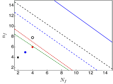
Figure 1: Estimates for the location of the conformal window of the SU(4) gauge theory with $N_{f}$ Dirac fermions in the fundamental representation and $n_{f}$ Majorana fermions in the sextet representation. The uppermost line is the limit of asymptotic freedom, where the 1-loop beta function changes sign. The other lines are various analytical estimates of the sill of the conformal window (see text). Blue circle: M6 model; red diamond: M11 model; black square: 2+2 model; open circle: 4+4 model, the subject of this paper. Only the lowest two lines are consistent with the IR fixed point that we find for the 4+4 model.

In this paper we move on to the “4+4 model,” where we increase the number of Dirac fermions in each representation from two to four. The 4+4 model has a number of desirable features. First, the M6 and M11 models can both be embedded into the 4+4 model, and can be reached by giving a subset of the fermions a (Dirac or Majorana) mass. In addition, as can be seen in the figure, the 4+4 model is much more likely to be close to, or even inside, the conformal window.

I.2 Method and summary of results

We extract the beta function and anomalous dimensions using a continuous renormalization group (RG) method [34, 35]. The length scale for this RG is $\sqrt{t}$, where $t$ is the parameter of a gradient flow (GF) generated by integrating a diffusion equation for the gauge field [39]. The GF running coupling is defined as [40]

$$g^{2}=\frac{\mathcal{N}}{C(t;L,T)}t^{2}\left\langle E(t)\right\rangle\ .$$ (1)

Here the energy density at scale $\sqrt{t}$ is $E=\frac{1}{4}G_{\mu\nu}^{a}G_{\mu\nu}^{a}$, where $G_{\mu\nu}^{a}$ is the flowed gauge field strength. $\mathcal{N}$ is a numerical factor which depends on the gauge group, and $C(t;L,T)$ is a correction for the finite dimensions $L,T$ of the volume being simulated (see below). Viewing the gradient flow as an RG transformation, the beta function is

$$\beta(g^{2})=-t\,\frac{\partial g^{2}}{\partial t}\ .$$ (2)

The extension of the GF technique to fermions was developed in Ref. [41], while the use of the continuous RG for obtaining anomalous dimensions of fermion operators was introduced in Ref. [42].

Figure 2: The $\beta$ function obtained with five different lattice gradient flows. All flows are the same in the continuum limit; their regions of validity are different, though overlapping. For details see Sec. II.

Our main findings are the beta function (Fig. 2), which shows an IR fixed point; the mass anomalous dimensions (Fig. 3); and the anomalous dimensions of the chimera operators with the lowest mass dimension, namely, three-fermion operators with no derivatives. The largest chimera anomalous dimension is shown in Fig. 4, while the other two are shown in Fig. 14. The IR fixed point places the model inside the conformal window. Moreover, the anomalous dimensions of the mass operators are large, for both representations, at the fixed point. Unfortunately, the anomalous dimensions of all chimera operators are fairly small at the fixed point, making it unlikely that the model can successfully account for a partially composite top quark.

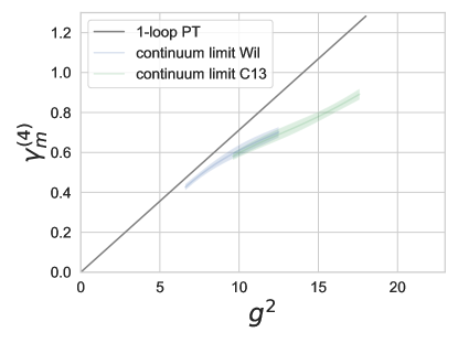
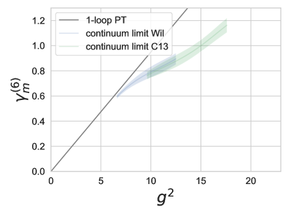
Figure 3: Anomalous dimensions of the two mass operators. Top: fundamental representation. Bottom: sextet representation. See Sec. III for details.

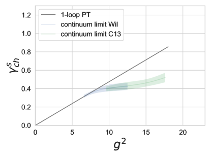
Figure 4: The largest chimera anomalous dimension, $\gamma^{s}_{ch}$. The other two chimera anomalous dimensions are smaller (see Fig. 14).

We obtain the flowed expectation values in Eq. (1) in the presence of a lattice cutoff, generating ensembles of the gauge field with numerical simulations. We present our lattice methods, including the calculation of the beta function and its extrapolation to the continuum limit, in Sec. II. The calculation of anomalous dimensions is the subject of Sec. III. We offer our conclusions in Sec. IV. Further technical details of the lattice calculation are given in the appendix.

II Gauge flow and the beta function

II.1 Lattice strategy

The lattice action, our simulation algorithm, and the ensembles we generated are described in the appendix. We use Wilson-clover fermions and tune the bare masses such that the fermions of both representations are essentially massless.

A new ingredient in the lattice action is a set of Pauli–Villars fields [43]. Without these, the presence of many fermion flavors, especially with smearing-improved gauge connections, generates a large screening effect in the effective action for the gauge field. In order to obtain a strong renormalized coupling, one would be pushed towards large bare coupling $g_{0}^{2}=N_{c}/\beta$. This, in turn, would cause large ultraviolet fluctuations. As a consequence, these systems often encounter phase transitions or other discontinuities, lattice artifacts that prevent the approach to the desired renormalized coupling, especially when the fermions are light. Our 4+4 system exhibited such a discontinuity when the original lattice action was used. The addition of Pauli–Villars fields weakens the induced term and allows us to reach much further into strong renormalized coupling.

As mentioned in the introduction, we use the continuous RG technique to determine the beta function. The 4+4 model that we simulate is a massless, asymptotically free lattice theory. The gradient flow acts as a transformation in coupling space: as the flow time $t$ is increased, irrelevant operators die out and the flow converges towards the renormalized trajectory (RT) emerging from the gaussian fixed point in the ultraviolet. Our task will be to ensure that, given a specific flow at a specific renormalized coupling, the flow has reached close enough to the RT that any remaining discretization effects can be removed by a simple extrapolation.

We begin by applying a gradient flow to the gauge field of every lattice configuration. In principle, extracting continuum results requires first taking the infinite-volume limit and then the continuum limit of zero lattice spacing $a$; the latter limit involves taking the dimensionless lattice flow time $t/a^{2}\to\infty$. Eschewing a formal infinite-volume limit, we focus on the continuum limit, which we extract from eight ensembles on a lattice volume of $24^{3}\times 48$ sites. The bare couplings of these ensembles were selected to range from weak to strong coupling. We have also generated ensembles on volume $28^{3}\times 56$ for two of the bare couplings; we use these to estimate finite-volume effects. By using lattice flow time $t/a^{2}\leq 3.4$ we have limited the finite volume effects to no more than a few percent.

II.2 Gauge flows

The continuum GF equation takes the form [39]

$$\frac{\partial B_{\mu}}{\partial t}=D_{\nu}G_{\nu\mu}\ ,$$ (3)

where $B_{\mu}$ is the flowed gauge field, and $G_{\nu\mu}$ the associated field strength. The initial condition of the flow is the dynamical gauge field, viz.,

$$B_{\mu}\big{|}_{t=0}=A_{\mu}\ .$$ (4)

The right-hand side of Eq. (3) is just $-\partial S_{g}/\partial B_{\mu}(x)$, where $S_{g}=\frac{1}{4}G_{\mu\nu}^{a}G_{\mu\nu}^{a}$ is the standard continuum gauge action in terms of the flowed field.

Flow	Sym	C43	Wil	C23	C13
$c_{p}$	5/3	4/3	1	2/3	1/3
$c_{r}$	$-1/12$	$-1/24$	0	$1/24$	$1/12$

Table 1: Lattice gradient flows. The first line gives the flow’s name used in this paper. “Sym” and “Wil” are the well-known Symanzik and Wilson flows. $c_{p}$ and $c_{r}$ are the coefficients of the plaquette and rectangle terms in the lattice action that generates each flow.

On the lattice, the continuum gauge field is replaced by the link variables $U_{\mu}(x)$. Each saved lattice configuration provides initial values for the gradient flow. We also need a discrete version of $\partial S_{g}/\partial B_{\mu}(x)$ for the right-hand side of the flow equation (see Ref. [39]). In this paper we apply five different gradient flows, each derived from a different discretization of the continuum action $S_{g}$. The lattice gauge action which generates each flow is a linear combination of the plaquette ($1\times 1$ Wilson loop) and rectangle ($1\times 2$ Wilson loop) terms, with coefficients shown in Table 1. For proper normalization in the weak-coupling limit, the plaquette and rectangle coefficients $c_{p}$ and $c_{r}$ are constrained by

$$c_{p}+8c_{r}=1\ .$$ (5)

As discussed in detail below, we have found that increasing $c_{p}$ from 1 gives rise to flows with relatively small discretization effects at weak bare coupling, while $c_{p}<1$ works well at strong bare coupling. In particular, we found the range of validity of the Symanzik flow to be limited to the weak coupling regime. We did not pursue the fully Symanzik-improved Zeuthen flow [44], as it is unlikely that further perturbative improvement would significantly change this conclusion.

Returning to Eq. (1) which defines the gradient flow coupling, the numerical constant here is

$$\mathcal{N}=\frac{128\pi^{2}}{3(N_{c}^{2}-1)}\simeq 28.4\ ,$$ (6)

for $N_{c}=4$. The finite-volume correction term $C(t;L,T)=1+\delta$ corrects for the zero modes of the gauge fields [40]. For volume $L^{3}\times T$ we have

$$\delta(t;L,T)=-\frac{\pi^{2}(8t)^{2}}{L^{3}T}+\vartheta\left(t/L^{2}\right)^{3}\vartheta\left(t/T^{2}\right)\ .$$ (7)

The correction $|\delta|$ is smaller than 0.005 for all our volumes in the useful ranges of $t$.

In addition, one has to select a discretization of the “energy” $E=S_{g}$, which is used to define the coupling in Eq. (1). We use three different discretizations, two of which correspond to the Symanzik (S) and Wilson (W) actions of Table 1. A third discretization is provided by the “clover” (C) operator. As explained below, we have found that the S operator gives the smoothest approach to the continuum limit, and so we will focus on results obtained using this operator.

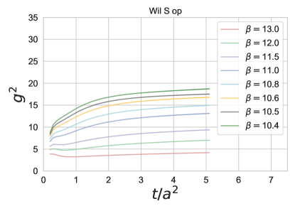
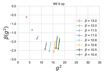
Figure 5: Results for the S operator measured in the Wilson flow. Top: Gradient flow coupling $g^{2}$ as a function of lattice flow time $t/a^{2}$. Bottom: $\beta(g^{2})$ vs. $g^{2}$ at flow times $2.4\leq t/a^{2}\leq 3.2$. Each open circle indicates the smallest flow time shown, $t/a^{2}=2.4$. Error bars in the top panel of this figure, as well as in Figs. 6 and 7, are too small to be visible.

II.3 Example flows and infinite volume limit

We generated each flow by numerically integrating a lattice version of the flow equation (3) in steps of $dt=0.01$. The energy $E$ of the flowed gauge field was recorded for the three operators S, W, and C, at intervals of $\Delta t=0.1$. The derivative in the bare beta function (2) was estimated with a five-point difference formula.

We show the raw flows for all eight of our $24^{3}\times 48$ ensembles in Fig. 5 for Wilson flow and in Fig. 6 for C13 flow. Both present the S operator. In each figure, the top panel shows the gradient flow coupling $g^{2}$ as a function of the lattice flow time $t/a^{2}$. The bottom panel shows the resulting raw beta function as a function of $g^{2}$ for a fixed interval of flow time $2.4\leq t/a^{2}\leq 3.2$.

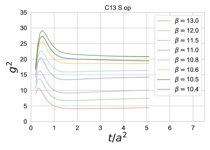
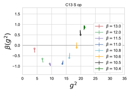
Figure 6: Similar to Fig. 5, for the S operator measured in C13 flow.

A comparison of the two figures reveals that the C13 flow reaches further into strong coupling than the Wilson flow: with the S operator, the former reaches $g^{2}\simeq 22$ while the latter reaches only $g^{2}\simeq 18$. There are similar distinctions among the three operators. For C13 flow, and within the above $t/a^{2}$ interval, the C operator reaches $g^{2}\simeq 18$ at our strongest bare coupling and the W operator reaches $g^{2}\simeq 20$, whereas the S operator reaches $g^{2}\simeq 22$ as just noted. In the lower panel of Fig. 6, we see that the beta function becomes positive for the largest couplings. Reaching larger values of the gradient flow coupling has direct bearing on the ability to confirm the existence of an IR fixed point.

Figures 5 and 6 show raw data—before extrapolation to the continuum. In Sec. II.4 and Sec. II.5 we will show that cutoff effects at strong coupling remain small for the S operator, and almost as small for the W operator. Moreover, the strongest attainable renormalized coupling of the C13 flow remains much larger than that of the Wilson flow in the continuum limit.

In Fig. 7 we examine the effect of increasing the lattice volume. We have generated two $28^{3}\times 56$ ensembles—at $\beta=11$ which is a weak (bare) coupling and at $\beta=10.5$ which is a strong coupling. In the top panel, we show the flows at these two bare couplings for the two volumes, again using C13 flow and the S operator. The change in $g^{2}$ and in its derivative due to changing the lattice volume is evidently small. The bottom panel shows the effect on the raw beta function. For both bare couplings, an increase in $L/a$ from 24 to 28 has the effect of shifting $g^{2}$ upward by about 0.1, leaving the $\beta$ function otherwise unchanged. We expect the extrapolation to infinite volume to be linear in $(a/L)^{4}$. It can be easily checked that the increase $L/a=24\to 28$ takes $(a/L)^{4}$ halfway to the limit. Hence, the expected change in $\beta(g^{2})$ is a horizontal shift by twice the amount seen in Fig. 7, with no qualitative change in the overall shape, including the existence of a fixed point. In the rest of this section we concentrate on our eight $24^{3}\times 48$ ensembles.

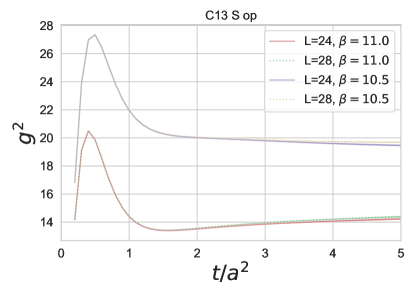
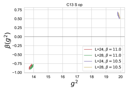
Figure 7: Volume comparison for the S operator measured in C13 flow in the $\beta=11.0$ and 10.5 ensembles. The volumes are $24^{3}\times 48$ and $28^{3}\times 56$. Top: Gradient flow coupling $g^{2}$ as a function of the lattice flow time $t/a^{2}$. Bottom: $\beta(g^{2})$ vs. $g^{2}$ at flow times $2.4\leq t/a^{2}\leq 3.2$.

II.4 Interpolation

In order to determine the continuum limit of $\beta(g^{2})$ we will extrapolate $t/a^{2}\to\infty$ at fixed $g^{2}$. In a theory with a rapidly running coupling the graph of the raw data for $\beta(g^{2})$, Fig. 5 or 6, would yield several ensembles that give different values for $\beta(g^{2})$ at any fixed coupling $g^{2}$ [34, 36]. We would then read off the corresponding flow time $t/a^{2}$ and $\beta(g^{2})$ for each ensemble, and take $t/a^{2}\to\infty$.

Since our theory runs slowly, each ensemble covers only a small range of $g^{2}$ and hence we have no overlaps between ensembles at any value of the coupling. Therefore, we have to interpolate $\beta(g^{2})$ vs. $g^{2}$ at fixed flow time—see Fig. 8. For a given flow time $t/a^{2}$, we identify the $(g^{2},\beta(g^{2}))$ pair on each ensemble. This gives us eight data points on each fixed-$t$ curve. To make vertical slices in $\beta(g^{2})$, we interpolate between ensembles at each fixed $t$. In weak coupling, $\beta(g^{2})\propto g^{4}$, and hence we use a polynomial interpolation even in strong coupling, $\beta(g^{2})/g^{4}=c_{0}+c_{1}g^{2}+c_{2}g^{4}+\cdots$, as detailed below. The curves plotted in Fig. 8 show the interpolations for the Wilson, C23 and C13 flows, using the S operator for the coupling.

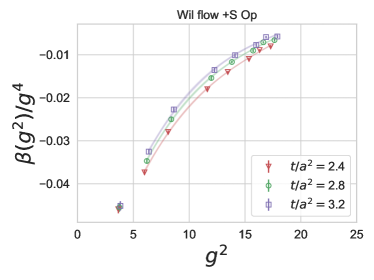
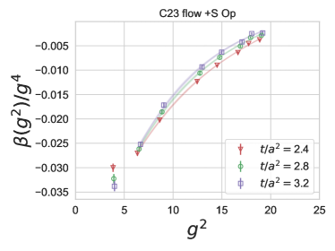
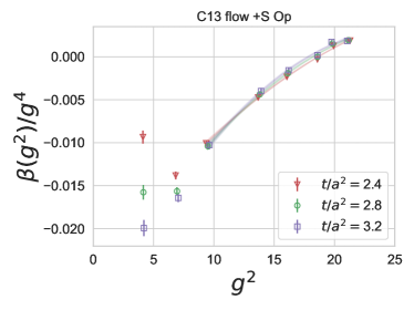
Figure 8: Interpolation of $\beta(g^{2})/g^{4}$ vs. $g^{2}$ for selected values of $t/a^{2}$ in Wilson flow (top left), C23 flow (top right), and C13 flow (bottom). The coupling $g^{2}$ is defined by the S operator, measured in the eight $24^{3}\times 48$ ensembles. In each plot, moving from left to right corresponds to stronger GF and bare couplings: the leftmost points come from $\beta=13$ and the rightmost from $\beta=10.4$. The curves connect only the points that were included in the interpolation.

Before performing each interpolation, we have to decide if we can use all eight data points. As can be seen in the figure, the C13 and C23 flows show rapid change with $t/a^{2}$ at the weakest bare couplings (the leftmost data points). We interpret this as indication that these flows require larger flow times in the weak coupling region to reach the vicinity of the RT. Interpolations with cubic, or even quartic, polynomials have poor $p$-values if we include all 8 data points. Dropping the left-most data point $\beta=13.0$ is sufficient to raise the $p$-value above 10% if we use a cubic interpolating polynomial for $\beta(g^{2})/g^{4}$. Even though Wilson flow shows smaller cutoff effects at $\beta=13.0$, for consistency we include only the seven ensembles at $\beta<13.0$ and use a cubic interpolation for both the Wilson and C23 flows. Moreover, for the C13 flow, it can be seen in the bottom panel of Fig. 8 that the $\beta=12.0$ point also shows large cutoff effects for the Symanzik operator. Hence, for this flow we discard $\beta=12$ from the interpolation as well, and use a quadratic interpolating polynomial to keep the same number of degrees of freedom in the interpolation as for the other flows.

The curves plotted in Fig. 8 connect only the data points that were included in the fits. As usual in interpolating data, in later stages of the analysis we will not use the interpolating curves outside the range of the data points that they connect.

The Symanzik and C43 flows (not shown in the figure) follow an opposite trend, exhibiting increasing cutoff effects in strong coupling. For those flows we drop the data point at the strongest bare coupling, $\beta=10.4$. Again, we use a cubic interpolating polynomial.

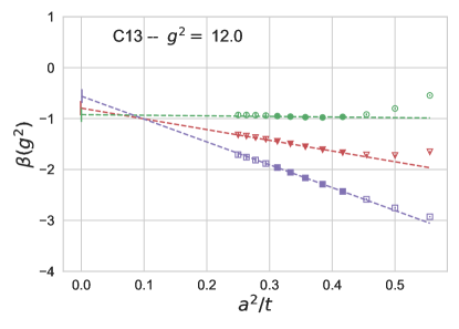
Figure 9: Extrapolations $a^{2}/t\to 0$ of $\beta(g^{2})$ at $g^{2}=12.0$. Data are (top to bottom) the S (green), W (red), and C (purple) operators measured in the C13 flow. Data plotted with open symbols have been dropped from the extrapolations.

II.5 Taking the continuum limit

We now turn to the final stage of our analysis, taking the continuum limit by extrapolating $t/a^{2}\to\infty$. Having constructed curves for $\beta(g^{2})$ for a selection of $t$ values, we now consider the $\beta$ surface as a set of curves $\beta(a^{2}/t)$ for a selection of $g^{2}$ values. At any given physical coupling $g^{2}$, the beta functions extracted from our different discretizations (S, W, C) must agree in the continuum limit; we will use this requirement to impose cuts on the range of $g^{2}$ where each flow can be trusted.

We show an example of the extrapolation process in Fig. 9, which shows the extrapolation of $\beta(g^{2})$ at $g^{2}=12.0$ for the C13 flow, for all three operators (S, W, C). The difference between the beta functions at finite lattice flow time $t/a^{2}$ obtained for any two operators should approach zero as $(a^{2}/t)^{\zeta}$, where $\zeta$ is the scaling exponent of the leading irrelevant operator. At weak coupling one expects $\zeta=1+O(g^{2})$, but in general the dependence on $g^{2}$ is not known. Our data do not allow us to resolve any statistically significant deviations from $\zeta=1$, and so we will assume that all cutoff effects scale linearly with $a^{2}/t$.

In Fig. 9 the data points plotted with open symbols are not included in the extrapolation. The smallest acceptable flow time depends on $g^{2}$—as well as, more generally, on the flow—reflecting how close we are to the RT. We also limit the maximum flow time to suppress finite volume effects. The remaining data give adequate linear extrapolations. We denote the extrapolated values by $\beta_{\text{S}},\beta_{\text{W}},\beta_{\text{C}}$.

We determine the error of each extrapolation with a bootstrap analysis. The closeness of the three extrapolated values indicates that the three operators give consistent results in this case. We will return to the precise condition for consistency shortly.

In Fig. 10 we show a compilation of continuum extrapolations. The three rows of the figure show extrapolations at $g^{2}=10.0,$ 14.0, and 17.0, while the three columns correspond, from left to right, to Wilson, C23, and C13 flows. Each panel depicts the extrapolation process for all three operators. A general feature revealed in the figure is that the slope of the extrapolation is always smallest for the S operator, with the W operator coming next. The C operator is last, having the largest slopes. This signals that discretization effects are smallest for the S operator. Combined with the other advantages of the S operator we have already discussed in Sec. II.3, this naturally leads to the choice of the S operator for our main result.

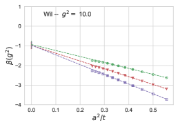
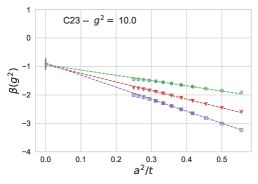
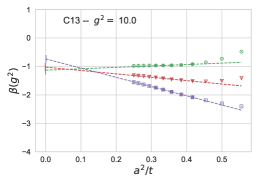
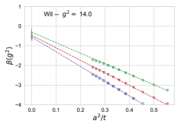
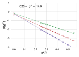
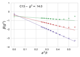
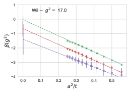
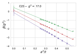
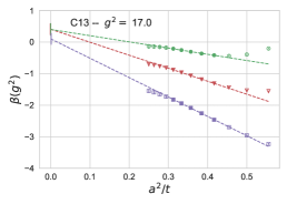
Figure 10: Extrapolations $a^{2}/t\to 0$ of $\beta(g^{2})$ for $g^{2}=10.0$ (top), 14.0 (middle), and 17.0 (bottom), which sample weak, intermediate, and strong couplings. At each value of $g^{2}$ we plot extrapolations for data from Wilson flow (left), C23 flow (center), and C13 flow (right). All data points come from flow times that belong to the interval $2.4\leq t/a^{2}\leq 3.2$. Color codes and symbols are the same as in Fig. 9.

It is evident in Fig. 10 that there are cases where the extrapolated values of the three operators are consistent with each other, whereas for other cases they are not (for example, the panel in lower left). While these plots give a general idea of the agreement of the extrapolations, they cannot directly be used to determine the consistency of the extrapolations. The reason is that data for the three operators are highly correlated. In order to correctly assess the level of agreement between any two extrapolations, their correlations must be taken into account.

We therefore base the criteria for consistency on the plots in Fig. 11, which include the effects of correlations. Since we will be basing our main result on the S operator, we plot red curves in each frame to represent $\pm\sqrt{2}\sigma_{\text{S}}$, where $\sigma_{\text{S}}$ is the error in $\beta_{\text{S}}$. The two bands in each frame are the $\pm 1\sigma$ bands for the correlated differences $\beta_{\text{S}}-\beta_{\text{W}}$ and $\beta_{\text{S}}-\beta_{\text{C}}$, which we also determine in the bootstrap analysis. We comment that these two bands are much narrower than the span between the red curves; this reflects the strong correlations among the three operators.

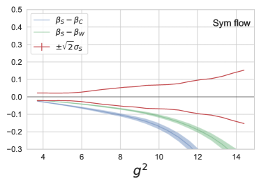
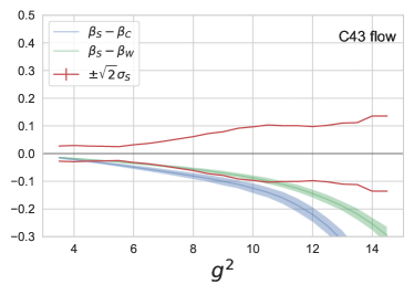
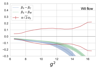
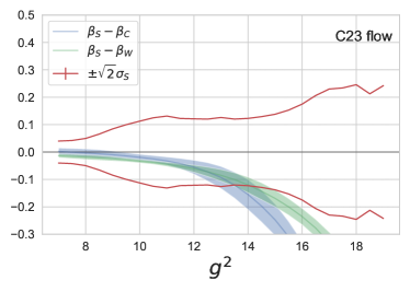
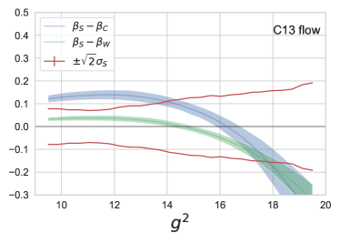
Figure 11: Comparing the differences $\beta_{\text{S}}-\beta_{\text{W}}$ (green) and $\beta_{\text{S}}-\beta_{\text{C}}$ (blue) with the standard deviation $\sigma_{\text{S}}$ of the S operator, at all physical couplings $g^{2}$ for each of the five flows. We require that the differences lie within the curves $\pm\sqrt{2}\sigma_{\text{S}}$ (red). The bounds of validity $g^{2}_{\text{min2}}$ and $g^{2}_{\text{max2}}$ in Tables 2 and 3 have been set accordingly.

The range of $g^{2}$ values where a given flow can be trusted is determined by the severity of discretization effects. As we have seen (e.g., in Figs. 9 and 10), the S operator shows the smallest discretization effects, with the W operator coming next. Hence we will determine this range by requiring consistency between $\beta_{\text{S}}$ and $\beta_{\text{W}}$. Table 2 shows the range of $g^{2}$ in which each set of flow data satisfies two constraints: (1) $g^{2}$ lies within the range of interpolation in Fig. 8, resulting in an interval $[g^{2}_{\text{min1}},g^{2}_{\text{max1}}]$; (2) the operators S and W give consistent values for the extrapolation to $a^{2}/t=0$, resulting in the smaller interval $[g^{2}_{\text{min2}},g^{2}_{\text{max2}}]$. The precise condition for consistency is that the mean value of $\beta_{\text{S}}-\beta_{\text{W}}$, represented by the green curves in Fig. 11, lies between the $\pm\sqrt{2}\sigma_{\text{S}}$ curves.

The beta function resulting from this analysis is the final result of this section. It is displayed in Fig. 2, and replicated in the top panel of Fig. 12. There is a nice agreement between the predictions of the different flows in their overlapping ranges. On the weak-coupling side, our result connects smoothly to perturbation theory. At strong coupling, we find an IR fixed point at $g^{2}$ somewhere between 15.5 and 16.

For completeness, we also examine the consequences of requiring consistency of all three operators. In this case, both of the differences $\beta_{\text{S}}-\beta_{\text{W}}$ and $\beta_{\text{S}}-\beta_{\text{C}}$ are required to lie between the $\pm\sqrt{2}\sigma_{\text{S}}$ curves, see Table 3. This results in a smaller range of validity for each flow, shown in the bottom panel of Fig. 12. It can be seen that now there is a gap between the coverage of the C43 and Wilson flows; a set of flows with $c_{p}$ and $c_{r}$ chosen between those of C43 and Wilson is needed to fill that gap. We note that for C13 flow, the differences $\beta_{\text{S}}-\beta_{\text{W}}$ and $\beta_{\text{S}}-\beta_{\text{C}}$ cross zero in the vicinity of the IR fixed point (bottom right panel of Fig. 11). In other words, the differences among the beta functions extracted from the extrapolations of the three operators are minimal near the fixed point. This lends further credibility to our determination of its existence and location.

Flow	$g^{2}_{\text{min1}}$	$g^{2}_{\text{max1}}$	$g^{2}_{\text{min2}}$	$g^{2}_{\text{max2}}$
Sym	3.7	13.6	3.7	4.0
C43	3.7	14.4	3.7	11.0
Wil	6.6	17.3	6.6	12.5
C23	6.8	18.9	6.8	14.0
C13	9.8	21.3	9.8	17.5

Table 2: Ranges of $g^{2}$ in which each flow is included in the final result for $\beta(g^{2})$. $g^{2}_{\text{min1}}$ and $g^{2}_{\text{max1}}$ result from limiting the ensembles included in the interpolations, while $g^{2}_{\text{min2}}$ and $g^{2}_{\text{max2}}$ come from further demanding consistency between the continuum extrapolations $\beta_{\text{S}}$ and $\beta_{\text{W}}$ (see Fig. 11). Since the second requirement does not constrain the $g^{2}$ range any further on the weak-coupling side, the $g^{2}_{\text{min1}}$ and $g^{2}_{\text{min2}}$ columns are identical. We quote $g^{2}_{\text{max2}}$ with a resolution of 0.5. The last two columns are the ranges reflected in the upper panel of Fig. 12 (and in Fig. 2).

Flow	$g^{2}_{\text{min1}}$	$g^{2}_{\text{max1}}$	$g^{2}_{\text{min2}}$	$g^{2}_{\text{max2}}$
Sym	3.7	13.6	(none)	(none)
C43	3.7	14.4	3.7	4.5
Wil	6.6	17.3	6.6	11.5
C23	6.8	18.9	6.8	13.5
C13	9.8	21.3	11.5	17.5

Table 3: Same as Table 2, but here the determination of $g^{2}_{\text{min2}}$ and $g^{2}_{\text{max2}}$ is based on consistency of $\beta_{\text{S}}$, $\beta_{\text{W}}$, and $\beta_{\text{C}}$, with results reflected in the lower panel of Fig. 12.

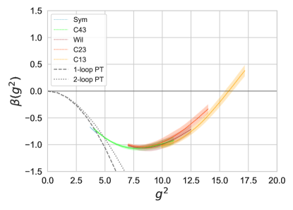
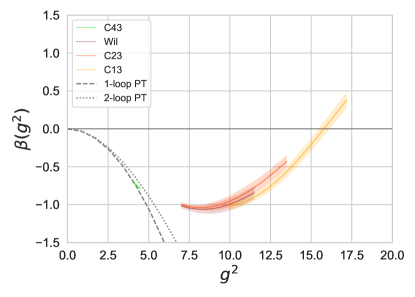
Figure 12: The $\beta$ function obtained with five different GF transformations. Both panels show the beta function derived from the S operator, but the ranges in $g^{2}$ allowed for each flow differ between them. For the top panel (identical to Fig. 2), only consistency between the S and W operators is required (Table 2). For the bottom panel, all three operators are required to be consistent (Table 3). In the bottom panel, there is a large gap between the $g^{2}$ regions of the C43 and Wilson flows—to bridge this gap a finer sequence of flows is needed. Also, there is no region of validity for the Symanzik flow, and thus it is not shown.

III Anomalous dimensions

In this section we compute the mass anomalous dimensions for the fundamental and sextet representations, as well as the anomalous dimensions of top-partner chimera operators, as functions of the renormalized coupling $g^{2}$. The anomalous dimensions in the infrared are then given by their values at the fixed point at $g^{2}\simeq 15.5$.

The gradient flow equation for a fermion field in the continuum is [41]

$$\frac{\partial\chi}{\partial t}=\Delta(t)\chi\ ,$$ (8)

where $\chi$ is the flowed fermion field. $\Delta$ is the covariant laplacian, constructed from the flowed gauge field at the same $t$. Similarly to the gauge field, the initial condition is

$$\chi(0)\big{|}_{t=0}=\psi\ ,$$ (9)

where $\psi$ is the dynamical fermion field.

There is a technical issue in the application of the continuous RG method to operators made out of fermion fields, described in Ref. [42]. Consider a two-point function of a flowed mesonic density $X^{\prime}$ with an unflowed source $X$,

$$\left\langle X(0)\,X^{\prime}(t)\right\rangle\sim t^{-(d+\eta+\gamma)/2}\ .$$ (10)

The scaling formula follows from the fact that here $X(0)$ is kept at $t=0$, while $X^{\prime}(t)$ is constructed from the flowed fermion fields at time $t$. The exponent reflects the classical dimension of the fermion bilinear, $d=3$; the anomalous dimension of the elementary fermion field, $\eta/2$; and the anomalous dimension of the meson operator, $\gamma$. The reason for the appearance of $\eta$ is that the gradient flow, unlike a blocking RG transformation, does not preserve the normalization of the fermion kinetic term.

One way to eliminate $\eta$ is to divide $\left\langle X(0)\,X^{\prime}(t)\right\rangle$ by the two-point function of a conserved current, whose anomalous dimension vanishes. We use the vector current, which scales according to (suppressing the vector index)

$$\left\langle V(0)\,V^{\prime}(t)\right\rangle\sim t^{-(d+\eta)/2}\ .$$ (11)

Defining the ratio

$$R(t)=\frac{\left\langle X(0)\,X^{\prime}(t)\right\rangle}{\left\langle V(0)\,V^{\prime}(t)\right\rangle}\ ,$$ (12)

we have

$$R(t)\sim t^{-\gamma/2}\ .$$ (13)

Now $\gamma$ can be extracted from the logarithmic derivative,

$$\gamma=-2\frac{t}{R}\,\frac{\partial R}{\partial t}\ .$$ (14)

We choose the operators $X$ and $X^{\prime}$ to lie in definite 3-volumes, separated by euclidean time $x_{4}$. We require $\sqrt{8t}\ll x_{4}$, meaning that the euclidean time separation must be large compared to the smearing of the operators by the flow. Once this condition is satisfied, the ratio $R(t)$ and the corresponding exponent $\gamma$ are expected to be independent of $x_{4}$.

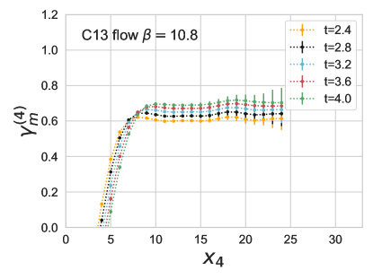
Figure 13: Examples of $x_{4}$ plateaus. Both panels show raw results for the mass anomalous dimension at $\beta=10.8$. Top: C13 flow, fundamental representation. Bottom: Wilson flow, sextet representation.

III.1 Mass anomalous dimensions

In the lattice calculation, for each representation we construct zero-momentum meson correlation functions,

$$C_{X}(x_{4},t)=\left\langle X(x_{4}^{0})\,X^{\prime}(x_{4}^{0}+x_{4},t)\right\rangle\ ,$$ (15)

where $X=S$ (scalar) or $P$ (pseudoscalar). The source $X$ is placed at euclidean time $x_{4}^{0}$, while the sink $X^{\prime}$ is separated by time $x_{4}$ from the source. To shorten autocorrelation times, we shift the source plane $x_{4}^{0}$ between successive lattice configurations of each ensemble. After fixing to Coulomb gauge, we construct the source $X$ using gaussian-smeared fermion fields with smearing radius $R_{0}=6$. We solve the Dirac equation using the conjugate gradient algorithm, and then flow the solution by integrating the fermion flow equation following Ref. [41]. We use point sinks, projected to $\vec{p}=0$. As for the gauge field, flowed correlation functions are recorded at interval $\Delta t=0.1$.

Having similarly computed the flowed two-point function of the vector current, we use Eq. (14) to determine the mass anomalous dimension $\gamma_{m}$ as a function of the euclidean time separation $x_{4}$ and the flow time $t$. Examples of raw results for $\gamma_{m}$ are shown in Fig. 13 for both representations. A new ingredient, clearly visible in the figure, is the $x_{4}$ plateaus. This provides a practical criterion for satisfying the condition $\sqrt{8t}\ll x_{4}$, and hence we extract the anomalous dimensions using values of $x_{4}$ inside the plateau, averaging over the range $11\leq x_{4}\leq 14$.

The rest of the calculation follows the same steps as for the beta function. We interpolate the raw results to obtain $\gamma_{m}$ as a function of $g^{2}$, and then use the interpolations $\gamma_{m}(t,g^{2})$ to take the continuum limit $a^{2}/t\to 0$ at fixed $g^{2}$.

Final results for the mass anomalous dimensions are shown in Fig. 3 above. In the weak-coupling region, the mass anomalous dimensions agree with one-loop perturbation theory,

$$\gamma_{m}=\frac{6g^{2}C_{2}}{16\pi^{2}}\ ,$$ (16)

where $C_{2}$ is the quadratic Casimir operator: $C_{2}=15/8$ for the fundamental representation and $C_{2}=5/2$ for the sextet representation. At larger couplings, the calculated mass anomalous dimensions move below the one-loop result. At the IR fixed point we have $\gamma_{m}^{(4)}\simeq 0.75$ for the fundamental representation and $\gamma_{m}^{(6)}\simeq 1.0$ for the sextet representation. Both are quite large, suggesting that while the 4+4 system is IR conformal, it is not too far from the conformal sill.

These results, like the beta function presented above, are based on data obtained on lattices of size $24^{3}\times 48$. We have carried out comparisons to the two $28^{3}\times 56$ ensembles, parallel to the analysis of $\beta(g^{2})$ in Sec. II.3. In a plot along the lines of Fig. 7, we find of course the same shift in $g^{2}$, but, again, no change in the data beyond the statistical error bars. Hence we expect $\gamma_{m}(g^{2})$ to move horizontally with the beta function as we approach the infinite-volume limit, with no other change. We obtain the same behavior for the chimera anomalous dimensions, presented below.

III.2 Chimera anomalous dimensions

Many different chimera operators can be used to create a top-partner state [46, 47]. We consider operators of the lowest possible mass dimension, which are three-fermion operators with no derivatives. To write them, we introduce Dirac fermions for the sextet representation, $\chi_{ABi}$, $i=1,\ldots,4$, where $i$ is a flavor index while $A,B=1,\ldots,4$, are the hypercolor indices, which are antisymmetrized. The fundamental representation fermions are denoted $\psi_{Aa}$, where $a=1,\ldots,4$ is also a flavor index. The three-fermion chimera operators are

$$B_{iab}^{IJ} = \epsilon_{ABCD}\,P_{I}\,\chi_{ABi}\,\left(\psi_{Ca}^{T}\,CP_{J}\,\psi_{Db}\right),$$ (17a)

$$B^{I}_{iab\mu} = \epsilon_{ABCD}\,P_{I}\,\gamma_{\mu}\chi_{ABi}\left(\psi^{T}_{Ca}C\gamma_{\mu}\gamma_{5}\psi_{Db}\right),\hskip 21.52771pt$$ (17b)

where the labels $I,J$ take the values $R,L$. Here $C$ is the charge-conjugation matrix and $P_{R,L}=(1\pm\gamma_{5})/2$. In Eq. (17b) there is no summation over $\mu$.

Projecting these operators onto the quantum numbers of the top quark depends on the details of the embedding of the Standard Model symmetries in the hypercolor (M6 or M11) model. For the M6 model, see Refs. [46, 47]. This will not concern us here.

We construct chimera two-point functions following closely Ref. [23]. All the chimera correlators we consider have the general form

$$C_{\pm}(x_{4},t)={\rm Tr}\left\langle B(x_{4}^{0}+x_{4},t)\,\bar{\Lambda}(x_{4}^{0})P_{\pm}\right\rangle\ ,$$ (18)

where $P_{\pm}={1\over 2}(1\pm\gamma_{4})$ are parity projectors. The source operator $\bar{\Lambda}$ is a quark-model creation operator for the top partner, which is kept at $t=0$ (for details, see Ref. [23]). The sink operator $B(x_{4}^{0}+x_{4},t)$ is one of the operators in Eq. (17). We use the same flowed fermion fields as for the mesons. As before, the sink is projected onto zero spatial momentum.

The correlation functions (18) are related by discrete (lattice) symmetries. First, the $B^{I}_{iab\mu}$ operators are related by hypercubic rotations; since we calculate correlation functions with $x_{4}$ dependence, we separate the $\mu=4$ operator from $\mu=1,2,3$ and lump the latter into a “space” component, viz.,

$$B^{sI}_{iab} = \frac{1}{3}\sum_{k=1}^{3}B^{I}_{iabk}\ ,$$ (19a)

$$B^{tI}_{iab} = B^{I}_{iab4}\ .$$ (19b)

In addition, the correlation functions (18) are related by the usual continuum discrete symmetries. Parity flips the chiral projectors, and so it takes, for example, $B^{RR}(\vec{p}=0,x_{4})\leftrightarrow B^{LL}(\vec{p}=0,x_{4})$. Euclidean time reversal likewise flips the parity projectors, and transforms the time component according to $x_{4}\leftrightarrow T-x_{4}$, where $T$ is the temporal extent of the lattice.

The outcome is that there are only three independent anomalous dimensions. We denote them $\gamma^{RR}_{ch}$ for $B^{RR}$ and $B^{LL}$; $\gamma^{RL}_{ch}$ for $B^{RL}$ and $B^{LR}$; and $\gamma^{s}_{ch}$ for $B^{sI}$ and $B^{tI}$.

Since each chimera operator consists of two fundamental and one sextet fermion, we normalize the flowed chimera two-point functions by constructing ratios [cf. Eq. (13)]

$$R_{\pm}(x_{4},t)=\frac{C_{\pm}(x_{4},t)}{C_{V}^{(4)}(x_{4},t)\sqrt{C_{V}^{(6)}(x_{4},t)}}\ .$$ (20)

Here $C_{V}^{(4)}(x_{4},t)$ and $C_{V}^{(6)}(x_{4},t)$ are the two-point functions of the fundamental and sextet vector currents. We then use Eq. (14) as before to extract the anomalous dimension.

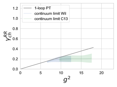
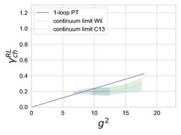
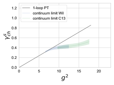
Figure 14: Anomalous dimensions of chimera operators. Top left: $\gamma^{RR}_{ch}$. Top right: $\gamma^{RL}_{ch}$. Bottom: $\gamma^{s}_{ch}$ (same plot as in Fig. 4).

Figure 14 shows our results for the three independent anomalous dimensions $\gamma^{RR}_{ch}$, $\gamma^{RL}_{ch}$ and $\gamma^{s}_{ch}$. The general behavior of each of them closely resembles that of the mass anomalous dimensions. At our weakest couplings, the anomalous dimensions agree with one-loop perturbation theory, whereas for larger couplings, the calculated anomalous dimensions fall below the one-loop curve. In addition, $\gamma^{RR}_{ch}$ and $\gamma^{RL}_{ch}$ agree within error, which is not required by symmetry.

The one-loop predictions are given by $\gamma=cg^{2}/(16\pi^{2})$, where $c=15/4$ for both $\gamma^{RR}_{ch}$ and $\gamma^{RL}_{ch}$, and $c=15/2$ for $\gamma^{s}_{ch}$ [48] (see also [49]). These anomalous dimensions happen to satisfy

$$\gamma^{RR}_{ch}:\gamma^{RL}_{ch}:\gamma^{s}_{ch}:\gamma_{m}^{(4)}:\gamma_{m}^{(6)}=1:1:2:3:4\ .$$ (21)

Thus, while at one loop $\gamma^{s}_{ch}$ is twice $\gamma^{RR}_{ch}$ or $\gamma^{RL}_{ch}$, it is still smaller than both of the mass anomalous dimensions. This pattern persists in our non-perturbative results. Indeed, the ratios (21) are roughly preserved near the fixed point as well, where $\gamma^{RR}_{ch}\approx\gamma^{RL}_{ch}\simeq 0.25$ and $\gamma^{s}_{ch}\simeq 0.5$.

IV Conclusions

As reported in this paper, we have employed lattice techniques to study the 4+4 model, an SU(4) gauge theory with four Dirac fermions in the fundamental representation and with eight Majorana fermions in the sextet representation. We used the continuous RG method, based on a gradient flow, to calculate the beta function and a number of important anomalous dimensions. Our lattice action includes a set of Pauli–Villars fields, which enable us to reach otherwise inaccessible strong couplings. We find that the 4+4 model has an infrared-stable fixed point at $g^{2}\simeq 15.5$.

We have dealt carefully with the continuum limit. Moreover, we have argued that finite-volume effects on both the beta function $\beta(g^{2})$ and the anomalous dimensions are limited to a common horizontal shift of a few percent, which leaves the anomalous dimensions at the infrared fixed point unchanged.

The M6 and M11 models of the Ferretti–Karateev list [7, 10] can be reached from the 4+4 model by giving large masses to a suitable subset of the fermions, while the fermion fields needed for the Ferretti–Karateev model itself are kept massless or given much smaller masses. Assuming that the Ferretti–Karateev model is below the conformal sill, it follows that the decoupling of the heavy fermions will trigger chiral symmetry breaking and confinement. The hypercolor scale $\Lambda_{HC}$ thus follows the heavy mass scale [16, 17, 18, 19].

We also find that the mass anomalous dimensions of both representations are quite large at the fixed point, even reaching $\gamma_{m}^{(6)}\simeq 1$ for the sextet representation. The anomalous dimensions of all top-partner chimera operators are smaller, reaching 0.5 or less. If one chooses masses for the fermions of the 4+4 model, as just discussed, to reach the M6 or the M11 model, the anomalous dimensions that govern the running of operators from the EHC scale down to the HC scale will still be controlled by the fixed point. The critical value of the chimera anomalous dimension, where suppression by a power of $\Lambda_{HC}/\Lambda_{EHC}$ is eliminated, is $\gamma=2$ (see for example Ref. [6]). Our results, then, indicate that these anomalous dimensions may not be large enough for a phenomenologically successful composite Higgs model.

*

Appendix A Lattice matters

A.1 Lattice action and simulation code

As in our previous work on the 2+2 model, we use a Wilson-clover fermion action, with a gauge-invariant kinetic term for each fermion species. We use normalized hypercubic (nHYP) smeared gauge links for the fundamental representation [50, 51]; gauge links for the sextet representation are constructed from these smeared links. The clover coefficient is set equal to unity for both fermion species [52, 53]. The gauge field action has the form $\beta S_{\text{plaq}}+\gamma S_{\text{NDS}}$, where $S_{\text{plaq}}$ is the usual plaquette action. $S_{\text{NDS}}$ is the nHYP dislocation suppressing action, a smeared action designed to reduce gauge-field roughness that would create large fermion forces in the molecular dynamics evolution [54]. We hold the ratio $\gamma/\beta=1/125$ fixed [20].

As discussed in Sec. II, in this work we have added a set of Pauli–Villars (PV) fields, which allow us to reach much further into strong renormalized coupling [43]. The PV action is the same Wilson-clover action as for the fermions, but the PV fields have opposite statistics. The ratio of PV to fermion fields is $3:1$, that is, we have 12 PV fields in each representation. The bare mass of the PV fields is kept at $am_{0}=1$ ($\kappa=1/10$) in order that they decouple in the continuum limit. This can be gauged by the mass of the ghost pion made out of two PV fields, which we find to be roughly equal to 2 in lattice units. This means that the effective gauge action induced by integrating over the PV fields is essentially local. For comparison, we note that the physical pions in both representations come out to have masses dictated by the volume, $m_{\pi}\simeq\pi/L$, where the lattice size is $L=24a$ or $28a$.

Our multi-representation code is a derivative of the MILC code [55]. We use three nested update levels with one Hasenbush preconditioning mass. The innermost level (level=0) contains the gauge update. Pseudofermion actions are simulated at level=1, which takes care of the upper end of the fermion spectrum, and at level=2, the outermost level, which takes care of the lower end of this spectrum. The PV fields are simulated at level=1, as is $S_{\text{NDS}}$.

A.2 Ensembles

For each value of the gauge coupling $\beta$, we determine the critical point $K_{c}=(\kappa_{4}^{c},\kappa_{6}^{c})$ by tuning the fermion masses to zero for both representations, as calculated from the axial Ward identities (AWI). We require the actual AWI masses to be $|m_{q}|\lesssim 0.002$, as we have seen that these masses are small enough to have negligible effect on the flow. The ensembles used in this work are shown in Table 4. In practice, we tuned to $K_{c}$ for each of our $24^{3}\times 48$ ensembles. In the $28^{3}\times 56$ ensembles we kept the same $(\kappa_{4},\kappa_{6})$ as for the smaller volume and verified that the AWI masses are practically unchanged.

$L/a$	$\beta$	$\phantom{X}\kappa_{4}$	$\phantom{X}\kappa_{6}$	lattices	$\phantom{XX}m_{q4}$	$\phantom{XX}m_{q6}$
24	10.4	0.12805	0.12905	35	$\phantom{-}0.0017(1)$	$-0.0003(1)$
24	10.5	0.12787	0.12876	25	$\phantom{-}0.0013(1)$	$\phantom{-}0.0011(1)$
24	10.6	0.12775	0.12855	35	$-0.0007(1)$	$\phantom{-}0.0005(1)$
24	10.8	0.12750	0.12804	25	$-0.0028(1)$	$\phantom{-}0.0040(1)$
24	11.0	0.12717	0.12777	25	$-0.0010(1)$	$\phantom{-}0.0015(1)$
24	11.5	0.12670	0.12724	25	$-0.0012(1)$	$-0.0009(1)$
24	12.0	0.12633	0.12680	45	$\phantom{-}0.00154(3)$	$\phantom{-}0.00139(3)$
24	13.0	0.12600	0.12640	45	$\phantom{-}0.00141(1)$	$\phantom{-}0.00010(1)$
28	10.5	0.12787	0.12876	25	$\phantom{-}0.0018(1)$	$\phantom{-}0.0015(1)$
28	11.0	0.12717	0.12777	25	$-0.00096(4)$	$\phantom{-}0.0016(1)$

Table 4: Parameters and fermion masses for the ensembles. The volume is $L^{3}\times T$, with $T=2L$. The fifth column gives the number of configurations that were used in the flow analysis. We saved a configuration every 5 trajectories (after equilibration). $m_{q4}$ and $m_{q6}$ are the AWI masses of the fundamental and sextet representations, respectively.

References

- Georgi and Kaplan [1984] H. Georgi and D. B. Kaplan, Composite Higgs and Custodial SU(2), Phys. Lett. 145B, 216 (1984).
- Dugan et al. [1985] M. J. Dugan, H. Georgi, and D. B. Kaplan, Anatomy of a Composite Higgs Model, Nucl. Phys. B254, 299 (1985).
- Kaplan [1991] D. B. Kaplan, Flavor at SSC energies: A New mechanism for dynamically generated fermion masses, Nucl. Phys. B365, 259 (1991).
- Contino [2011] R. Contino, The Higgs as a Composite Nambu-Goldstone Boson, in Physics of the large and the small, TASI 09, proceedings of the Theoretical Advanced Study Institute in Elementary Particle Physics, Boulder, Colorado, USA, 1-26 June 2009 (2011) pp. 235–306, arXiv:1005.4269 [hep-ph] .
- Bellazzini et al. [2014] B. Bellazzini, C. Csáki, and J. Serra, Composite Higgses, Eur. Phys. J. C74, 2766 (2014), arXiv:1401.2457 [hep-ph] .
- Panico and Wulzer [2016] G. Panico and A. Wulzer, The Composite Nambu-Goldstone Higgs, Lect. Notes Phys. 913 (2016), arXiv:1506.01961 [hep-ph] .
- Ferretti and Karateev [2014] G. Ferretti and D. Karateev, Fermionic UV completions of Composite Higgs models, JHEP 03, 077, arXiv:1312.5330 [hep-ph] .
- Ferretti [2014] G. Ferretti, UV Completions of Partial Compositeness: The Case for a SU(4) Gauge Group, JHEP 06, 142, arXiv:1404.7137 [hep-ph] .
- Ferretti [2016] G. Ferretti, Gauge theories of Partial Compositeness: Scenarios for Run-II of the LHC, JHEP 06, 107, arXiv:1604.06467 [hep-ph] .
- Belyaev et al. [2017] A. Belyaev, G. Cacciapaglia, H. Cai, G. Ferretti, T. Flacke, A. Parolini, and H. Serodio, Di-boson signatures as Standard Candles for Partial Compositeness, JHEP 01, 094, arXiv:1610.06591 [hep-ph] .
- Vecchi [2017] L. Vecchi, A dangerous irrelevant UV-completion of the composite Higgs, JHEP 02, 094, arXiv:1506.00623 [hep-ph] .
- Cacciapaglia et al. [2021] G. Cacciapaglia, S. Vatani, and C. Zhang, The Techni-Pati-Salam Composite Higgs, Phys. Rev. D 103, 055001 (2021), arXiv:2005.12302 [hep-ph] .
- Bando et al. [1988] M. Bando, T. Kugo, and K. Yamawaki, Nonlinear Realization and Hidden Local Symmetries, Phys. Rept. 164, 217 (1988).
- Hill and Simmons [2003] C. T. Hill and E. H. Simmons, Strong Dynamics and Electroweak Symmetry Breaking, Phys. Rept. 381, 235 (2003), [Erratum: Phys.Rept. 390, 553–554 (2004)], arXiv:hep-ph/0203079 .
- Kaplan et al. [2009] D. B. Kaplan, J.-W. Lee, D. T. Son, and M. A. Stephanov, Conformality Lost, Phys. Rev. D 80, 125005 (2009), arXiv:0905.4752 [hep-th] .
- Brower et al. [2016] R. C. Brower, A. Hasenfratz, C. Rebbi, E. Weinberg, and O. Witzel, Composite Higgs model at a conformal fixed point, Phys. Rev. D 93, 075028 (2016), arXiv:1512.02576 [hep-ph] .
- Hasenfratz et al. [2017] A. Hasenfratz, C. Rebbi, and O. Witzel, Large scale separation and resonances within LHC range from a prototype BSM model, Phys. Lett. B 773, 86 (2017), arXiv:1609.01401 [hep-ph] .
- Witzel and Hasenfratz [2019] O. Witzel and A. Hasenfratz (Lattice Strong Dynamics), Constructing a composite Higgs model with built-in large separation of scales, PoS LATTICE2019, 115 (2019), arXiv:1912.12255 [hep-lat] .
- Appelquist et al. [2021] T. Appelquist et al. (Lattice Strong Dynamics), Near-conformal dynamics in a chirally broken system, Phys. Rev. D 103, 014504 (2021), arXiv:2007.01810 [hep-ph] .
- Ayyar et al. [2018a] V. Ayyar, T. DeGrand, M. Golterman, D. C. Hackett, W. I. Jay, E. T. Neil, Y. Shamir, and B. Svetitsky, Spectroscopy of SU(4) composite Higgs theory with two distinct fermion representations, Phys. Rev. D97, 074505 (2018a), arXiv:1710.00806 [hep-lat] .
- Ayyar et al. [2018b] V. Ayyar, T. Degrand, D. C. Hackett, W. I. Jay, E. T. Neil, Y. Shamir, and B. Svetitsky, Baryon spectrum of SU(4) composite Higgs theory with two distinct fermion representations, Phys. Rev. D97, 114505 (2018b), arXiv:1801.05809 [hep-ph] .
- Ayyar et al. [2018c] V. Ayyar, T. DeGrand, D. C. Hackett, W. I. Jay, E. T. Neil, Y. Shamir, and B. Svetitsky, Finite-temperature phase structure of SU(4) gauge theory with multiple fermion representations, Phys. Rev. D97, 114502 (2018c), arXiv:1802.09644 [hep-lat] .
- Ayyar et al. [2018d] V. Ayyar, T. DeGrand, D. C. Hackett, W. I. Jay, E. T. Neil, Y. Shamir, and B. Svetitsky, Partial compositeness from baryon matrix elements on the lattice, (2018d), arXiv:1812.02727 [hep-ph] .
- Ayyar et al. [2019] V. Ayyar, M. F. Golterman, D. C. Hackett, W. Jay, E. T. Neil, Y. Shamir, and B. Svetitsky, Radiative Contribution to the Composite-Higgs Potential in a Two-Representation Lattice Model, Phys. Rev. D 99, 094504 (2019), arXiv:1903.02535 [hep-lat] .
- Golterman et al. [2021] M. Golterman, W. I. Jay, E. T. Neil, Y. Shamir, and B. Svetitsky, Low-energy constant in a two-representation lattice theory, Phys. Rev. D 103, 074509 (2021), arXiv:2010.01920 [hep-lat] .
- Cossu et al. [2019] G. Cossu, L. Del Debbio, M. Panero, and D. Preti, Strong dynamics with matter in multiple representations: gauge theory with fundamental and sextet fermions, Eur. Phys. J. C 79, 638 (2019), arXiv:1904.08885 [hep-lat] .
- Del Debbio et al. [2023] L. Del Debbio, A. Lupo, M. Panero, and N. Tantalo, Multi-representation dynamics of SU(4) composite Higgs models: chiral limit and spectral reconstructions, Eur. Phys. J. C 83, 220 (2023), arXiv:2211.09581 [hep-lat] .
- Bennett et al. [2018] E. Bennett, D. K. Hong, J.-W. Lee, C. J. D. Lin, B. Lucini, M. Piai, and D. Vadacchino, Sp(4) gauge theory on the lattice: towards SU(4)/Sp(4) composite Higgs (and beyond), JHEP 03, 185, arXiv:1712.04220 [hep-lat] .
- Bennett et al. [2019] E. Bennett, D. K. Hong, J.-W. Lee, C. J. D. Lin, B. Lucini, M. Piai, and D. Vadacchino, Sp(4) gauge theories on the lattice: dynamical fundamental fermions, JHEP 12, 053, arXiv:1909.12662 [hep-lat] .
- Bennett et al. [2022] E. Bennett, D. K. Hong, H. Hsiao, J.-W. Lee, C. J. D. Lin, B. Lucini, M. Mesiti, M. Piai, and D. Vadacchino, Lattice studies of the Sp(4) gauge theory with two fundamental and three antisymmetric Dirac fermions, Phys. Rev. D 106, 014501 (2022), arXiv:2202.05516 [hep-lat] .
- Hsiao et al. [2022] H. Hsiao, E. Bennett, D. K. Hong, J.-W. Lee, C. J. D. Lin, B. Lucini, M. Piai, and D. Vadacchino, Spectroscopy of chimera baryons in a Sp(4) lattice gauge theory, (2022), arXiv:2211.03955 [hep-lat] .
- Bennett et al. [2023] E. Bennett, J. Holligan, D. K. Hong, H. Hsiao, J.-W. Lee, C. J. D. Lin, B. Lucini, M. Mesiti, M. Piai, and D. Vadacchino, Sp() Lattice Gauge Theories and Extensions of the Standard Model of Particle Physics (2023) arXiv:2304.01070 [hep-lat] .
- Kim et al. [2020] B. S. Kim, D. K. Hong, and J.-W. Lee, Into the conformal window: Multirepresentation gauge theories, Phys. Rev. D 101, 056008 (2020), arXiv:2001.02690 [hep-ph] .
- Hasenfratz and Witzel [2020] A. Hasenfratz and O. Witzel, Continuous renormalization group function from lattice simulations, Phys. Rev. D 101, 034514 (2020), arXiv:1910.06408 [hep-lat] .
- Hasenfratz and Witzel [2019] A. Hasenfratz and O. Witzel, Continuous function for the SU(3) gauge systems with two and twelve fundamental flavors, PoS LATTICE2019, 094 (2019), arXiv:1911.11531 [hep-lat] .
- Peterson et al. [2022] C. T. Peterson, A. Hasenfratz, J. van Sickle, and O. Witzel, Determination of the continuous function of SU(3) Yang-Mills theory, PoS LATTICE2021, 174 (2022), arXiv:2109.09720 [hep-lat] .
- Hasenfratz et al. [2023] A. Hasenfratz, C. T. Peterson, J. van Sickle, and O. Witzel, parameter of the SU(3) Yang-Mills theory from the continuous function, (2023), arXiv:2303.00704 [hep-lat] .
- Fodor et al. [2018] Z. Fodor, K. Holland, J. Kuti, D. Nogradi, and C. H. Wong, A new method for the beta function in the chiral symmetry broken phase, EPJ Web Conf. 175, 08027 (2018), arXiv:1711.04833 [hep-lat] .
- Lüscher [2010] M. Lüscher, Properties and uses of the Wilson flow in lattice QCD, JHEP 08, 071, [Erratum: JHEP 03, 092 (2014)], arXiv:1006.4518 [hep-lat] .
- Fodor et al. [2012] Z. Fodor, K. Holland, J. Kuti, D. Nogradi, and C. H. Wong, The Yang-Mills gradient flow in finite volume, JHEP 11, 007, arXiv:1208.1051 [hep-lat] .
- Lüscher [2013] M. Lüscher, Chiral symmetry and the Yang–Mills gradient flow, JHEP 04, 123, arXiv:1302.5246 [hep-lat] .
- Carosso et al. [2018] A. Carosso, A. Hasenfratz, and E. T. Neil, Nonperturbative Renormalization of Operators in Near-Conformal Systems Using Gradient Flows, Phys. Rev. Lett. 121, 201601 (2018), arXiv:1806.01385 [hep-lat] .
- Hasenfratz et al. [2021] A. Hasenfratz, Y. Shamir, and B. Svetitsky, Taming lattice artifacts with Pauli-Villars fields, Phys. Rev. D 104, 074509 (2021), arXiv:2109.02790 [hep-lat] .
- Ramos and Sint [2016] A. Ramos and S. Sint, Symanzik improvement of the gradient flow in lattice gauge theories, Eur. Phys. J. C 76, 15 (2016), arXiv:1508.05552 [hep-lat] .
- Hasenfratz and Witzel [2021] A. Hasenfratz and O. Witzel, Dislocations under gradient flow and their effect on the renormalized coupling, Phys. Rev. D 103, 034505 (2021), arXiv:2004.00758 [hep-lat] .
- Golterman and Shamir [2015] M. Golterman and Y. Shamir, Top quark induced effective potential in a composite Higgs model, Phys. Rev. D91, 094506 (2015), arXiv:1502.00390 [hep-ph] .
- Golterman and Shamir [2018] M. Golterman and Y. Shamir, Effective potential in ultraviolet completions for composite Higgs models, Phys. Rev. D97, 095005 (2018), arXiv:1707.06033 [hep-ph] .
- DeGrand and Shamir [2015] T. DeGrand and Y. Shamir, One-loop anomalous dimension of top-partner hyperbaryons in a family of composite Higgs models, Phys. Rev. D92, 075039 (2015), arXiv:1508.02581 [hep-ph] .
- Buarque Franzosi and Ferretti [2019] D. Buarque Franzosi and G. Ferretti, Anomalous dimensions of potential top-partners, SciPost Phys. 7, 027 (2019), arXiv:1905.08273 [hep-ph] .
- Hasenfratz and Knechtli [2001] A. Hasenfratz and F. Knechtli, Flavor symmetry and the static potential with hypercubic blocking, Phys. Rev. D64, 034504 (2001), arXiv:hep-lat/0103029 [hep-lat] .
- Hasenfratz et al. [2007] A. Hasenfratz, R. Hoffmann, and S. Schaefer, Hypercubic smeared links for dynamical fermions, JHEP 05, 029, arXiv:hep-lat/0702028 [hep-lat] .
- Bernard and DeGrand [2000] C. W. Bernard and T. A. DeGrand, Perturbation theory for fat link fermion actions, Lattice field theory. Proceedings, 17th International Symposium, Lattice’99, Pisa, Italy, June 29-July 3, 1999, Nucl. Phys. Proc. Suppl. 83, 845 (2000), arXiv:hep-lat/9909083 [hep-lat] .
- Shamir et al. [2011] Y. Shamir, B. Svetitsky, and E. Yurkovsky, Improvement via hypercubic smearing in triplet and sextet QCD, Phys. Rev. D83, 097502 (2011), arXiv:1012.2819 [hep-lat] .
- DeGrand et al. [2014] T. DeGrand, Y. Shamir, and B. Svetitsky, Suppressing dislocations in normalized hypercubic smearing, Phys. Rev. D90, 054501 (2014), arXiv:1407.4201 [hep-lat] .
- [55] MILC Collaboration, http://www.physics.utah.edu/~detar/milc/.