End-to-End Feasible Optimization Proxies
for Large-Scale Economic Dispatch

Abstract

The paper proposes a novel End-to-End Learning and Repair (E2ELR) architecture for training optimization proxies for economic dispatch problems. E2ELR combines deep neural networks with closed-form, differentiable repair layers, thereby integrating learning and feasibility in an end-to-end fashion. E2ELR is also trained with self-supervised learning, removing the need for labeled data and the solving of numerous optimization problems offline. E2ELR is evaluated on industry-size power grids with tens of thousands of buses using an economic dispatch that co-optimizes energy and reserves. The results demonstrate that the self-supervised E2ELR achieves state-of-the-art performance, with optimality gaps that outperform other baselines by at least an order of magnitude.

Nomenclature

-A Sets and indices

• buses

• branches

• generators

-B Variables

• Energy dispatch of generator $g$

• Reserve dispatch of generator $g$

• Thermal limit violation on branch $e$

-C Parameters

• Active power demand at bus $i$

• Production cost function of generator $g$

• Lower and upper thermal limits on branch $e$

• Thermal violation penalty cost

• Maximum output of generator $g$

• Maximum reserve of generator $g$

• Minimum reserve requirement

• PTDF matrix

• Vector of all zeros

• Vector of all ones

I Introduction

The optimal power flow (OPF) is a fundamental problem in power systems operations. Its linear approximation, the DC-OPF model, underlies most electricity markets, especially in the US. For instance, MISO uses a security-constrained economic dispatch (SCED) in their real-time markets, which has the DC-OPF model at its core [1]. The continued growth in renewable and distributed energy resources (DERs) has caused an increase in operational uncertainty. This creates need for new methodologies and operating practices that can quantify and manage risk in real time [2, 3]. Nevertheless, quantifying the operational risk of a transmission system requires executing in the order of $10^{3}$ Monte Carlo (MC) simulations, each requiring the solution of multiple (typically in the hundreds) economic dispatch problems [4, 3]. To fit within the constraints of actual operations, real-time risk assessment would thus require solving hundreds of thousands of economic dispatch problems within a matter of seconds. This represents a 100,000x speedup over current optimization technology, which can typically solve economic dispatch problems in a few seconds.

In recent years, there has been a surge of interest, both from the power systems and Machine-Learning (ML) communities, in developing optimization proxies for OPF, i.e., ML models that approximate the input-output mapping of OPF problems. The main idea is that, once trained, these proxies can be used to generate high-quality solutions orders of magnitude faster than traditional optimization solvers. This capability allows to evaluate a large number of scenarios fast, thereby enabling real-time risk assessment.

There are however three major obstacles to the deployment of optimization proxies: feasibility, scalability and adaptability. First, ML models are not guaranteed to satisfy the physical and engineering constraints of the model. This causes obvious issues if, for instance, the goal is to use a proxy to evaluate whether the system is able to operate in a safe state. Several approaches have been proposed in the past to address the feasibility of ML predictions, each of which has some advantages and limitations. Second, most results in ML for power systems has considered systems with up to 300 buses, far from the size of actual systems that contain thousands of buses. Moreover, the resulting techniques have not been proven to scale or be accurate enough on large-scale networks. Third, power grids are not static: the generator commitments and the grid topology evolve over time, typically on an hourly basis [5]. Likewise, the output of renewable generators such as wind and solar generators is non-stationary, which may degrade the performances of ML models. Therefore, it is important to be able to (re)train models fast, typically within a few hours at most. This obviously creates a computational bottleneck for approaches that rely on the offline solving of numerous optimization problems to generate training data.

Despite significant interest from the community, no approach has thus far addressed all three challenges (feasibility, scalability and adaptability) in a unified way. This paper addresses this gap by proposing an End-to-End Learning and Repair (E2ELR) architecture for a (MISO-inspired) economic dispatch (ED) formulation where the prediction and feasibility restoration are integrated in a single ML pipeline and trained jointly. The E2ELR-ED architecture guarantees feasibility, i.e., it always outputs a feasible solution to the economic dispatch. The E2ELR-ED architecture achieves these results through closed-form repair layers. Moreover, through the use of self-supervised learning, the E2ELR-ED architecture is scalable, both for training and inference, and is found to produce near-optimal solutions to systems with tens of thousands of buses. Finally, the use of self-supervised learning also avoids the costly data-generation process of supervised-learning methods. This allows to re-train the model fast, smoothly adapting to changing operating parameters and system conditions. The contributions of the paper can therefore be summarized as follows:

• The paper proposes a novel E2ELR architecture with closed-form, differentiable repair layers, whose output is guaranteed to satisfy power balance and reserve requirements. This is the first architecture to consider reserve requirements, and to offer feasibility guarantees without restrictive assumptions.

• The E2ELR model is trained in an end-to-end fashion that combines learning and feasibility restoration, making the approach scalable to large-scale systems. This contrasts to traditional approaches that restore feasibility at inference time, which increases computing time and induces significant losses in accuracy.

• The paper proposes self-supervised learning to eliminate the need for offline generation of training data. The proposed E2ELR can thus be trained from scratch in under an hour, even for large systems. This allows to adapt to changing system conditions by re-training the model periodically.

• The paper conducts extensive numerical experiments on systems with up to 30,000 buses, a 100x increase in size compared to most existing studies. The results demonstrate that the proposed self-supervised E2ELR architecture is highly scalable and outperforms other approaches.

The rest of the paper is organized as follows. Section II surveys the relevant literature. Section III presents an overview of the E2ELR architecture and contrast it with existing approaches. Section IV presents the problem formulation and the E2ELR architecture in detail. Section V presents supervised and self-supervised training. Section VI describes the experiment setting, and Section VII reports numerical results. Section VIII concludes the paper and discusses future research directions.

II Related works

II-A Optimization Proxies for OPF

The majority of the existing literature on OPF proxies employs Supervised Learning (SL) techniques. Each data point $(x,y)$ consists of an OPF instance data ($x$) and its corresponding solution ($y$). The training data is obtained by solving a large number –usually tens of thousands– of OPF instances offline. The SL paradigm has successfully been applied both in the linear DCOPF [6, 7, 8, 9, 5, 10, 11] and nonlinear, non-convex ACOPF [12, 13, 14, 15, 16, 17, 18, 19, 20, 21, 22, 23, 24, 25, 26, 27, 28, 29] settings. In almost all the above references, the generator commitments and grid topology are assumed to be fixed, with electricity demand being the only source of variability. Therefore, these OPF proxies must be re-trained regularly to capture the hourly changes in commitments and topology that occur in real-life operations [5]. In a SL setting, this comes at a high computational cost because of the need to re-generate training data. Recent works consider active sampling techniques to reduce this burden [30, 31]. References [14, 24, 25, 26] consider graph neural network (GNN) architectures to accommodate topology changes, however, numerical results are only reported on small networks with at most 300 buses.

Self-Supervised Learning (SSL) has emerged as an alternative to SL that does not require labeled data [32, 33, 34]. Namely, training OPF proxies in a self-supervised fashion does not require the solving of any OPF instance offline, thereby removing the need for (costly) data generation. In [32], the authors train proxies for ACOPF where the training loss consists of the objective value of the predicted solution, plus a penalty term for constraint violations. A similar approach is used in [33] in conjunction with Generative Adversarial Networks (GANs). More recently, Park et al [34] jointly train a primal and dual network by mimicking an Augmented Lagrangian algorithm. Predicting Lagrange multipliers allows for dynamically adjusting the constraint violation penalty terms in the loss function. Current results suggest that SSL-based proxies can match the accuracy of SL-based proxies.

II-B Ensuring Feasibility

One major limitation of ML-based OPF proxies is that, in general, the predicted OPF solution violates physical and engineering constraints that govern power flows and ensure safe operations. To alleviate this issue, [13, 9] use a restricted OPF formulation to generate training data, wherein the OPF feasible region is artificially shrunk to ensure that training data consists of interior solutions. In [9], this strategy is combined with a verification step (see also [35]) to ensure the trained models have sufficient capacity to reach a universal approximation. Nevertheless, this requires solving bilevel optimization problems, which is very cumbersome: [9] reports training times in excess of week for a 300-bus system. In addition, it may not be possible to shrink the feasible region in general, e.g., when the lower and upper bounds are the same.

In the context of DCOPF, [6, 5, 10, 11] exploit the fact that an optimal solution can be quickly recovered from an (optimal) active set of constraints. A combined classification-then-regression architecture is proposed in [5], wherein a classification step identifies a subset of variables to be fixed to their lower or upper bound, thus reducing the dimension of the regression task. In [6, 11], the authors predict a full active set, and recover a solution by solving a system of linear equations. Similarly, [10] combine decision trees and active set-based affine policies. Importantly, active set-based approaches may yield infeasible solutions when active constraints are incorrectly classified [11]. Furthermore, correctly identifying an optimal active set becomes harder as problem size increases.

A number of prior work have investigated physics-informed models (e.g., [13, 15, 16, 5, 19, 18, 32, 33]). This approach augments the training loss function with a term that penalizes constraint violations, and is efficient at reducing – but not eliminating – constraint violations. To better balance feasibility and [15, 16] dynamically adjust the penalty coefficient using ideas from Lagrangian duality. In a similar fashion, [34] uses a primal and a dual networks: the latter predicts optimal Lagrange multipliers, which inform the loss function used to train the former.

Although physics-informed models generally exhibit lower constraint violations, they still do not produce feasible solutions. Therefore, several works combine an (inexact) OPF proxy with a repair step that restores feasibility. A projection step is used in [7, 15], wherein the (infeasible) predicted solution is projected onto the feasible set of OPF. In DCOPF, this projection is a convex (typically linear or quadratic) problem, whereas the load flow model used in [15] for ACOPF is non-convex. Instead of a projection step, [13] uses an AC power flow solver to recover voltage angles and reactive power dispatch from predicted voltage magnitudes and generator dispatches. This is typically (much) faster than a load flow. However, while the resulting solution satisfies the power flow equations (assuming the solver converges), it may not satisfy all engineering constraints such as the thermal limits of the lines. Finally, [36] uses techniques from state estimation to restore feasibility for ACOPF problems. This approach has not been applied in the context of OPF proxies.

The development of implicit differentiable layers [37] makes it possible to embed feasibility restoration inside the proxy architecture itself, thereby removing the need for post-processing [17, 38, 39]. This allows to train models in an end-to-end fashion, i.e., the predicted solution is guaranteed to satisfy constraints. For instance, [38] implement the aforementioned projection step as an implicit layer. However, because they require solving an optimization problem, these implicit layers incur a very high computational cost, both during training and testing. Equality constraints can also be handled implicitly via so-called constraint completion [17, 39]. Namely, a set of independent variables is identified, and dependent variables are recovered by solving the corresponding system of equations, thereby satisfying equality constraints by design. Note that constraint completion requires the set of independent variables to be the same across all instances, which may not hold in general. For instance, changes in generator commitments and/or grid topology may introduce dependencies between previously-independent variables. The difference between [17] and [39] lies in the treatment of inequality constraints. On the one hand, [17] replace a costly implicit layer with cheaper gradient unrolling, which unfortunately does not guarantee feasibility. On the other hand, [39] use gauge functions to define a one-to-one mapping between the unit hypercube, which is easy to enforce with sigmoid activations, and the set of feasible solutions, thereby guaranteeing feasibility. Nevertheless, the latter approach is valid only under restrictive assumptions: all constraints are convex, the feasible set is bounded, and a strictly feasible point is available for each instance.

II-C Scalability Challenges

There exists a significant gap between the scale of actual power grids, and those used in most academic studies: the former are typically two orders of magnitude larger than the latter. On the one hand, actual power grids comprise thousands to tens of thousands of buses [40, 41]. On the other hand, most academic studies only consider small, artificial power grids with no more than 300 buses. Among the aforementioned works, [11] considers a synthetic NYISO grid with 1814 buses, and only [16, 5, 27] report results on systems with more than 6,000 buses. This discrepancy makes it difficult to extrapolate most existing findings to scenarios encountered in the industry. Indeed, actual power grids exhibit complex behaviors not necessarily captured by small-scale cases [40].

III Overview of the Proposed Approach

The paper addresses the shortcomings in current literature by combining learning and feasibility restoration in a single E2ELR architecture. Figure 1 illustrates the proposed architecture (Figure 1e), alongside existing architectures from previous works. In contrast to previous works, the proposed E2ELR uses specialized, closed-form repair layers that allow the architecture to scale to industry-size systems. E2ELR is also trained with self-supervised learning, alleviating the need for labeled data and the offline solving of numerous optimization problems. As a result, even for the largest systems considered, the self-supervised E2ELR is trained from scratch in under an hour, and achieves state-of-the-art performance, outperforming other baselines by an order of magnitude. Note that E2ELR also bridges the gap between academic DCOPF formulations and those used in the industry, by including reserve requirements in the ED formulation. To the best of the authors’ knowledge, this is the first work to explicitly consider –and offer feasibility guarantees for– reserve requirements in the context of optimization proxies. Moreover, the repair layers are guaranteed to satisfy power balance and reserve requirements for any combination of min/max generation limits (see Theorems 1 and 2). This allows to accommodate variations in operating parameters such as min/max limits and commitment status of generators, a key aspect of real-life systems overlooked in existing literature.

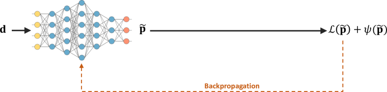
(a) The vanilla DNN architecture without feasibility restoration.

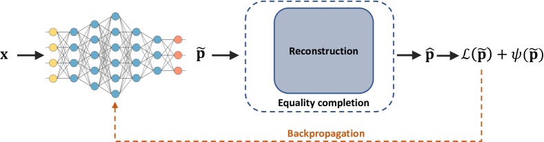
(b) The DeepOPF architecture [7]. The output $\mathbf{\hat{p}}$ may violate inequality constraints.

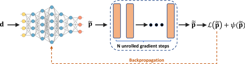
(c) The DC3 architecture with unrolled gradient [17]. The output $\mathbf{\tilde{\tilde{p}}}$ may violate inequality constraints.

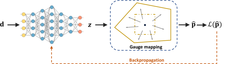
(d) The LOOP-LC architecture [39]. The DNN outputs a latent vector $\mathbf{z}\in[0,1]^{n}$, which is mapped onto a feasible $\mathbf{\hat{p}}$ via a gauge mapping.

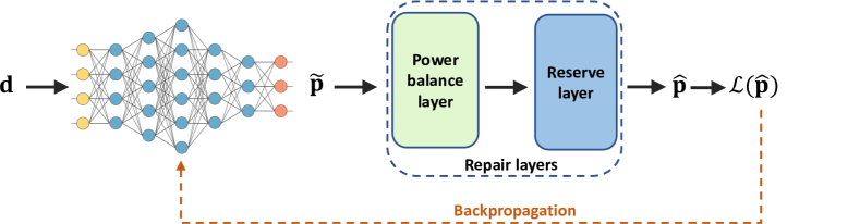
(e) The proposed end-to-end feasible architecture. The output $\mathbf{\hat{p}}$ satisfies all hard constraints.

Figure 1: Optimization proxy architectures for DCOPF

IV End-to-end feasible proxies for DCOPF

This section presents the Economic Dispatch (ED) formulation considered in the paper, and introduces new repair layers for power balance and reserve requirement constraints. The repair layers are computationally efficient and differentiable: they can be implemented in standard machine-learning libraries, enabling end-to-end feasible optimization proxies.

IV-A Problem Formulation

The paper considers an ED formulation with reserve requirements. It is modeled as a linear program of the form

$$\min_{\mathbf{p},\mathbf{r},\xi_{\text{th}}}\quad c(\mathbf{p})+M_{\text{th}}\|\xi_{\text{th}}\|_{1}$$ (1a)

s.t. $$\mathbf{e}^{\top}\mathbf{p}=\mathbf{e}^{\top}\mathbf{d},$$ (1b)

$$\mathbf{e}^{\top}\mathbf{r}\geq R,$$ (1c)

$$\mathbf{p}+\mathbf{r}\leq\mathbf{\bar{p}},$$ (1d)

$$\mathbf{0}\leq\mathbf{p}\leq\mathbf{\bar{p}},$$ (1e)

$$\mathbf{0}\leq\mathbf{r}\leq\mathbf{\bar{r}},$$ (1f)

$$\mathbf{\underline{f}}-\xi_{\text{th}}\leq\Phi(\mathbf{p}-\mathbf{d})\leq\mathbf{\bar{f}}+\xi_{\text{th}},$$ (1g)

$$\xi_{\text{th}}\geq\mathbf{0}.$$ (1h)

Constraints (1b) and (1c) are the global power balance and minimum reserve requirement constraints, respectively. Constraints (1d) ensure that each generator reserves can be deployed without violating their maximum capacities. Constraints (1e) and (1f) enforce minimum and maximum limits on each generator energy and reserve dispatch. Without loss of generality, the paper assumes that each bus has exactly one generator, each generator minimum output is zero, and $\bar{r}_{g}\leq\bar{p}_{g},\forall g$. Constraints (1g) express the thermal constraints on each branch using a Power Transfer Distribution Factor (PTDF) representation. In this paper, the thermal constraints are soft constraints, i.e., they can be violated but doing so incurs a (high) cost. This is modeled via artificial slack variables $\xi_{\text{th}}$ which are penalized in the objective. Treating thermal constraints as soft is in line with economic dispatch formulations used by system operators to clear electricity markets in the US [42, 43]. The PTDF-based formulation is also the state-of-the-art approach used in industry [42, 41]. In typical operations, only a small number of these constraints are active at the optimum. Therefore, efficient implementations add thermal constraints (1g) lazily.

The hard constraints in Problem (1) are the bounds on energy and reserve dispatch, the maximum output, the power balance (1b) and the reserve requirements (1c). Note that bounds on individual variables can easily be enforced in a DNN architecture e.g., via clamping or sigmoid activation. However, it is not trivial to simultaneously satisfy variable bounds, power balance and reserve requirements. To address this issue, the rest of this section introduces new, computationally efficient repair layers.

IV-B The Power Balance Repair Layer

The proposed power balance repair layer takes as input an initial dispatch vector $\mathbf{p}$, which is assumed to satisfy the min/max generation bounds (1e), and outputs a dispatch vector $\tilde{\mathbf{p}}$ that satisfies constraints (1e) and (1b). Formally, let $D\,{=}\,\mathbf{e}^{\top}\mathbf{d}$, and denote by $\mathcal{H}$ and $\mathcal{S}_{D}$ the following hypercube and hypersimplex

$$\mathcal{H} =\left\{\mathbf{p}\in\mathbb{R}^{n}\ \middle|\ \mathbf{0}\leq\mathbf{p}\leq\mathbf{\bar{p}}\right\},$$ (2)

$$\mathcal{S}_{D} =\left\{\mathbf{p}\in\mathbb{R}^{n}\ \middle|\ \mathbf{0}\leq\mathbf{p}\leq\mathbf{\bar{p}},\ \mathbf{e}^{\top}\mathbf{p}=D\right\}.$$ (3)

Note that $\mathcal{H}$ is the feasible set of constraints (1e), while $\mathcal{S}_{D}$ is the feasible set of constraints (1b) and (1e). The proposed power balance repair layer, denoted by $\mathcal{P}$, is given by

$$\begin{array}[]{rl}\mathcal{P}(\mathbf{p})&=\left\{\begin{array}[]{ll}(1-\eta^{\uparrow})\mathbf{p}+\eta^{\uparrow}\mathbf{\bar{p}}&\text{if }\mathbf{e}^{\top}\mathbf{p}<D\\ (1-\eta^{\downarrow})\mathbf{p}+\eta^{\downarrow}\mathbf{0}&\text{if }\mathbf{e}^{\top}\mathbf{p}\geq D\end{array}\right.\end{array}$$ (7)

where $\mathbf{p}\,{\in}\,\mathcal{H}$, and $\eta^{\uparrow}$, $\eta^{\downarrow}$ are defined as follows:

$$\eta^{\uparrow} =\frac{\mathbf{e}^{\top}\mathbf{d}-\mathbf{e}^{\top}\mathbf{p}}{\mathbf{e}^{\top}\mathbf{\bar{p}}-\mathbf{e}^{\top}\mathbf{p}}, \eta^{\downarrow} =\frac{\mathbf{e}^{\top}\mathbf{p}-\mathbf{e}^{\top}\mathbf{d}}{\mathbf{e}^{\top}\mathbf{p}-\mathbf{e}^{\top}\mathbf{0}}.$$ (8)

Theorem 1 below shows that $\mathcal{P}$ is well-defined.

Theorem 1.

Assume that $0<\mathbf{e}^{\top}\mathbf{d}=D<\mathbf{e}^{\top}\mathbf{\bar{p}}$ and $\mathbf{p}\in\mathcal{H}$.
Then, $\mathcal{P}(\mathbf{p})\in\mathcal{S}_{D}$.

Proof.

Let $\mathbf{\tilde{p}}\,{=}\,\mathcal{P}(\mathbf{p})$, and assume $\mathbf{e}^{\top}\mathbf{p}\,{<}\,D$; the case $\mathbf{e}^{\top}\mathbf{p}\,{\geq}\,D$ is treated similary. It follows that $\eta^{\uparrow}\,{\in}\,[0,1]$, i.e., $\mathbf{\tilde{p}}$ is a convex combination of $\mathbf{p}$ and $\mathbf{\bar{p}}$. Thus, $\mathbf{\tilde{p}}\in\mathcal{H}$. Then,

$$\mathbf{e}^{\top}\mathbf{\tilde{p}} =(1-\eta^{\uparrow})\mathbf{e}^{\top}\mathbf{p}+\eta^{\uparrow}\mathbf{e}^{\top}\bar{\mathbf{p}}$$

$$=\eta^{\uparrow}(\mathbf{e}^{\top}\bar{\mathbf{p}}-\mathbf{e}^{\top}\mathbf{p})+\mathbf{e}^{\top}\mathbf{p}$$

$$=\frac{D-\mathbf{e}^{\top}\mathbf{p}}{\mathbf{e}^{\top}\mathbf{\bar{p}}-\mathbf{e}^{\top}\mathbf{p}}(\mathbf{e}^{\top}\bar{\mathbf{p}}-\mathbf{e}^{\top}\mathbf{p})+\mathbf{e}^{\top}\mathbf{p}$$

$$=D-\mathbf{e}^{\top}\mathbf{p}+\mathbf{e}^{\top}\mathbf{p}=D.$$

Thus, $\mathbf{\tilde{p}}$ satisfies the power balance and $\mathbf{\tilde{p}}\in\mathcal{S}_{D}$. ∎

Note that feasible predictions are not modified: if $\mathbf{p}\in\mathcal{S}_{D}$, then $\mathcal{P}(\mathbf{p})=\mathbf{p}$. The edge cases not covered by Theorem 1 are handled as follows. When $D\leq 0$ (resp. $D\geq\mathbf{e}^{\top}\mathbf{\bar{p}}$), each generator is set to its lower (resp. upper) bound; this can be achieved by clamping $\eta^{\uparrow}$ (resp. $\eta^{\downarrow}$) to $[0,1]$. If these inequalities are strict, Problem (1) is trivially infeasible, and $\mathcal{P}(\mathbf{p})$ is the solution that minimizes power balance violations.

The power balance layer is illustrated in Figure 2, for a two-generator system. The layer has an intuitive interpretation as a proportional response mechanism. Indeed, if the initial dispatch $\mathbf{p}$ has an energy shortage, i.e., $\mathbf{e}^{\top}\mathbf{p}\,{<}\,D$, the output of each generator is increased by a fraction $\eta^{\uparrow}$ of its upwards headroom. Likewise, if the initial dispatch has an energy surplus, i.e., $\mathbf{e}^{\top}\mathbf{p}\,{>}\,D$, the output of each generator is decreased by a fraction $\eta^{\downarrow}$ of it downwards headroom.

Figure 2: Illustration of the power balance layer with input $\mathbf{p}$ and output $\mathbf{\tilde{p}}$. Left: $\mathbf{e}^{\top}\mathbf{p}\,{<}\,D$ (energy shortage) and generators’ dispatches are increased. Right: $\mathbf{e}^{\top}\mathbf{p}\,{>}\,D$ (energy surplus) and generators’ dispatches are decreased.

Note that $\mathcal{S}_{D}$ is defined by the combination of bound constraints and one equality constraint. Other works such as [17, 39] handle the latter via equality completion. While this approach satisfies the equality constraint by design, the recovered solution is not guaranteed to satisfy min/max bounds, and may fail to do so in general. In contrast, under the only assumption that $\mathbf{p}\in\mathcal{H}$, the proposed layer (7) jointly enforces both constraints, thus alleviating the need for the gradient unrolling of [17] or gauge mapping of [39]. Finally, the proposed layer generalizes to hypersimplices of the form

$$\left\{x\in\mathbb{R}^{n}\ \middle|\ l\leq x\leq u,a^{T}x=b\right\},$$ (9)

where $a\in\mathbb{R}^{n},b\in\mathbb{R}$ and $l\leq u\in\mathbb{R}^{n}$ are finite bounds.

IV-C The Reserve Repair Layer

This section presents the proposed reserve feasibility layer, which ensures feasibility with respect to constraints (1c), (1d), and (1f). The approach first builds a compact representation of these constraints by projecting out the reserve variables $\mathbf{r}$. This makes it possible to consider only the $\mathbf{p}$ variables, which in turn enables a computationally efficient and interpretable feasibility restoration. Let $\mathbf{p}\in\mathcal{S}_{D}$ be fixed, and consider the problem of maximizing total reserves, which reads

$$\max_{\mathbf{r}}\quad \mathbf{e}^{\top}\mathbf{r}$$ (10a)

s.t. $$\mathbf{r}\leq\bar{\mathbf{p}}-\mathbf{p},$$ (10b)

$$0\leq\mathbf{r}\leq\bar{\mathbf{r}}.$$ (10c)

Since $\mathbf{p}$ is fixed, constraints (10b)–(10c) reduce to simple variable bounds on the $\mathbf{r}$ variables. It then immediately follows that the optimal solution to Problem (10) is given by

$$r^{*}_{g}=\min\{\bar{r}_{g},\bar{p}_{g}-p_{g}\},\ \forall g.$$ (11)

This observation is used to project out the reserve variables as stated in Lemma 1 below.

Lemma 1.

Let $\mathbf{p}\in\mathcal{S}_{D}$. There exists reserves $\mathbf{r}$ such that $(\mathbf{p},\mathbf{r})$ is feasible for Problem (1) if and only if

$$\sum_{g}\min\{\bar{r}_{g},\bar{p}_{g}-p_{g}\}\geq R.$$ (12)

Proof.

The proof follows from the fact that $(\mathbf{p},\mathbf{r})$ is feasible for Problem (1) if and only if Problem (10) has an objective value not smaller than $R$. Substituting the optimal solution given in Eq. (11), this last statement is exactly equivalent to $\sum_{g}\min\{\bar{r}_{g},\bar{p}_{g}-p_{g}\}\geq R$. ∎

The proposed reserve repair layer builds on the power balance repair layer of Section IV-B, and on the compact formulation of Eq. (12). Namely, it takes as input $\mathbf{p}\,{\in}\,\mathcal{S}_{D}$, and outputs $\mathcal{R}(\mathbf{p})\,{\in}\,\mathcal{S}_{D}$ that satisfies Eq. (12). Given $\mathcal{R}(\mathbf{p})$, reserve variables can be recovered in $O(|\mathcal{G}|)$ time using Eq. (11).

The reserve repair layer is presented in Algorithm 1. First, a tentative reserve allocation is computed using Eq. 11, and the corresponding reserve shortage $\Delta_{R}$ is computed. Then, generators are split into two groups $G^{\uparrow}$ and $\mathcal{G}^{\downarrow}$. Generators in $\mathcal{G}^{\uparrow}$ are those for which constraint (1f) is active: their dispatch can be increased without having to reduce their reserves. Generators in $\mathcal{G}^{\downarrow}$ are those for which constraint (1d) is active: one must reduce their energy dispatch to increase their reserves. Then, the algorithm computes the maximum possible increase ($\Delta^{\uparrow}$) and decrease ($\Delta^{\downarrow})$ in energy dispatch for the two groups. Finally, each generator energy dispatch is increased (resp. decreased) proportionately to its increase (resp. decrease) potential so as to meet total reserve requirements. The total increase in energy dispatch is equal to the total decrease, so that power balance is always maintained.

Algorithm 1 Reserve Repair Layer

0:  Initial prediction $\mathbf{p}\in\mathcal{S}_{D}$, maximum limits $\mathbf{\bar{p}},\mathbf{\bar{r}}$, reserve requirement $R$

1:  $\Delta_{R}\leftarrow R-\sum_{g}\min\{\bar{r}_{g},\bar{p}_{g}-p_{g}\}$

2:  $\mathcal{G}^{\uparrow}\leftarrow\left\{g\ \middle|\ p_{g}\leq\bar{p}_{g}-\bar{r}_{g}\right\}$

3:  $\mathcal{G}^{\downarrow}\leftarrow\left\{g\ \middle|\ p_{g}>\bar{p}_{g}-\bar{r}_{g}\right\}$

4:  $\Delta^{\uparrow}\leftarrow\sum_{g\in\mathcal{G}^{\uparrow}}(\bar{p}_{g}-\bar{r}_{g})-p_{g}$

5:  $\Delta^{\downarrow}\leftarrow\sum_{g\in\mathcal{G}^{\downarrow}}p_{g}-(\bar{p}_{g}-\bar{r}_{g})$

6:  $\Delta\leftarrow\max(0,\min(\Delta_{R},\Delta^{\uparrow},\Delta^{\downarrow}))$

7:  $\alpha^{\uparrow}\leftarrow\Delta/\Delta^{\uparrow}$, $\alpha^{\downarrow}\leftarrow\Delta/\Delta^{\downarrow}$,

8:  Energy dispatch adjustment

$$\tilde{p}_{g} =\left\{\begin{array}[]{ll}(1-\alpha^{\uparrow})p_{g}+\alpha^{\uparrow}(\bar{p}_{g}-\bar{r}_{g})&\forall g\in\mathcal{G}^{\uparrow}\\ (1-\alpha^{\downarrow})p_{g}+\alpha^{\downarrow}(\bar{p}_{g}-\bar{r}_{g})&\forall g\in\mathcal{G}^{\downarrow}\end{array}\right.$$

9:  return $\mathcal{R}(\mathbf{p})=\mathbf{\tilde{p}}$

The reserve feasibility recovery is illustrated in Figure 3 for a two-generator system. While it is easy to verify that $\mathcal{R}(\mathbf{p})\in\mathcal{S}_{D}$, it is less clear whether $\mathcal{R}(\mathbf{p})$ satisfies Eq. (12). Theorem 2 provides the theoretical guarantee that either $\mathcal{R}(\mathbf{p})$ satisfies Eq. (12), or no feasible solution to Problem (1) exists. Because of space limitations, the proof is given in [44].

Theorem 2.

Let $\mathbf{p}\in\mathcal{S}_{D}$. Then, $\mathcal{R}(\mathbf{p})\in\mathcal{S}_{D}$. Furthermore, $\mathcal{R}(\mathbf{p})$ satisfies Eq. (12) if and only if Problem (1) is feasible.

Theorem 2 also provides a fast proof of (in)feasibility for Problem (1): it suffices to evaluate $\mathcal{R}(\mathbf{p})$ for any $\mathbf{p}\in\mathcal{S}_{D}$ and check Eq. (12). This can have applications beyond optimization proxies, e.g., to quickly evaluate a large number of scenarios for potential reserve violations. Finally, note that the results of Theorems 1 and 2 hold for any value of the maximum limits $\mathbf{\bar{p}},\bar{\mathbf{r}}$ and reserve requirement $R$.

Figure 3: Illustration of the reserve feasibility layer for $\mathbf{\bar{p}}{=}(1,1)$, $\mathbf{\bar{r}}{=}(0.5,0.5)$, $D{=}1.1$, $R{=}0.8$ and the initial prediction $\mathbf{p}{=}(0.15,0.95)$. The recovered feasible dispatch is $\mathbf{\tilde{p}}{=}(0.4,0.7)$. Top: effect of the layer in the $(p_{1},p_{2})$ space. Bottom: effect of the layer on each generator (individually). The active constraint is shown in red. Generator $1$ is in $\mathcal{G}^{\uparrow}$ and generator 2 is in $\mathcal{G}^{\downarrow}$.

IV-D End-to-end Feasible Training

The repair layers are combined with a Deep Neural Network (DNN) architecture to provide an end-to-end feasible ML model, i.e., a differentiable architecture that is guaranteed to output a feasible solution to Problem (1) (if and only if one exists). The resulting architecture is illustrated in Figure 4. The proxy takes as input the vector of nodal demand $\mathbf{d}$. The DNN architecture consists of fully-connected layers with ReLU activation, and a final layer with sigmoid activations to enforce bound constraints on $\mathbf{p}$. Namely, the last layer outputs $\mathbf{z}\in[0,1]^{n}$, and $\mathbf{\tilde{p}}=\mathbf{z}\cdot\mathbf{\bar{p}}$ satisfies constraints (1e). Then, this initial prediction $\mathbf{\tilde{p}}$ is fed to the repair layers that restore the feasibility of the power balance and reserve requirements. The final prediction $\mathbf{\hat{p}}$ is feasible for Problem (1).

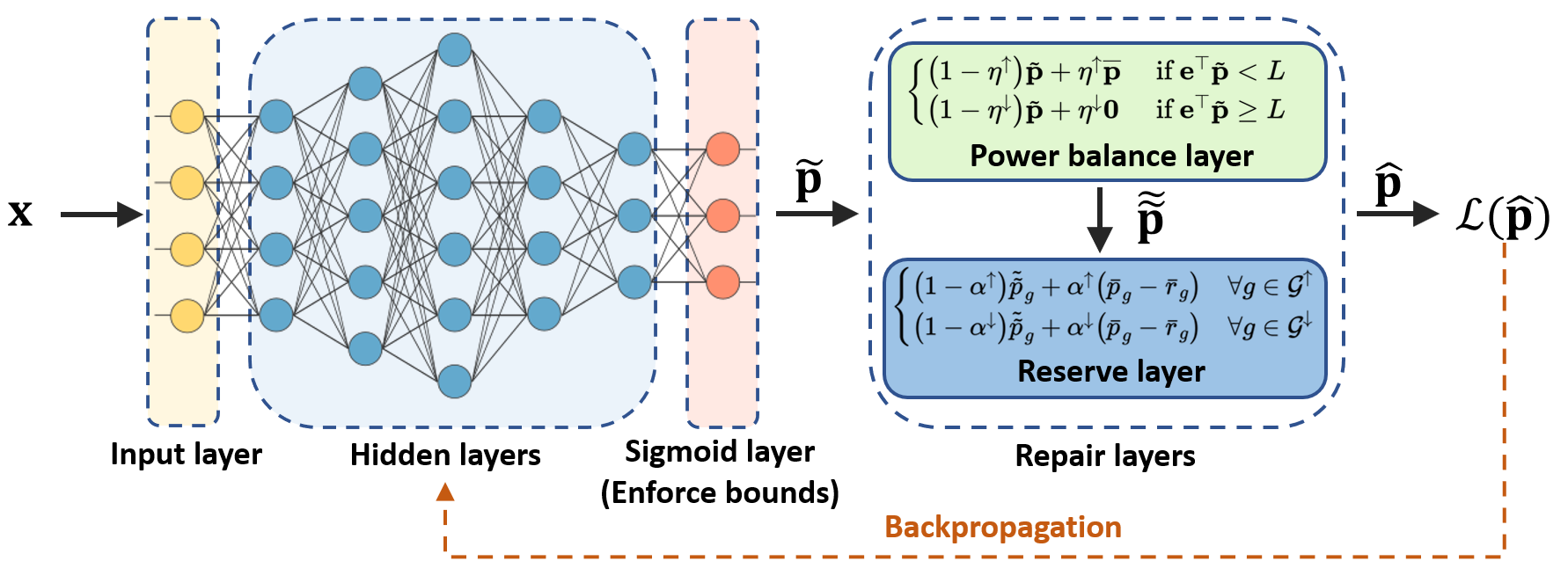
Figure 4: The Proposed End-To-End Feasible Architecture.

The power balance and reserve feasibility layers only require elementary arithmetic and logical operations, all of which are supported by mainstream ML libraries like PyTorch and TensorFlow. Therefore, it can be implemented as a layer of a generic artificial neural network model trained with back-propagation. Indeed, these layers are differentiable almost everywhere with informative (sub)gradients. Finally, the proposed feasibility layers can be used as a stand-alone, post-processing step to restore feasibility of any dispatch vector that satisfies generation bounds. This can be used for instance to build fast heuristics with feasibility guarantees.

V Training methodology

This section describes the supervised learning (SL) and self-supervised learning (SSL) approaches for training optimization proxies, which are illustrated in Figure 5. The difference between these two paradigms lies in the choice of loss function for training, not in the model architecture. Denote by $\mathbf{x}$ the input data of Problem (1), i.e.,

$$\mathbf{x}=(c,\mathbf{d},R,\mathbf{\bar{p}},\mathbf{\bar{r}},\Phi,\mathbf{\underline{f}},\mathbf{\bar{f}},M_{\text{th}}),$$

and recall, from Section IV-C, that it is sufficient to predict the (optimal) value of variables $\mathbf{p}$. Denote by $f_{\theta}$ the mapping of a DNN architecture with trainable parameters $\theta$; given an input $\mathbf{x}$, $f_{\theta}(\mathbf{x})$ predicts a generator dispatch $f_{\theta}(\mathbf{x})=\hat{\mathbf{p}}$.

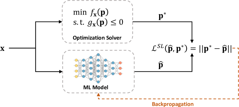
(a) Supervised Learning: the loss function $\mathcal{L}^{SL}$ measures the distance to an optimal solution $\mathbf{p}^{*}$, which is computed offline by an optimization solver.

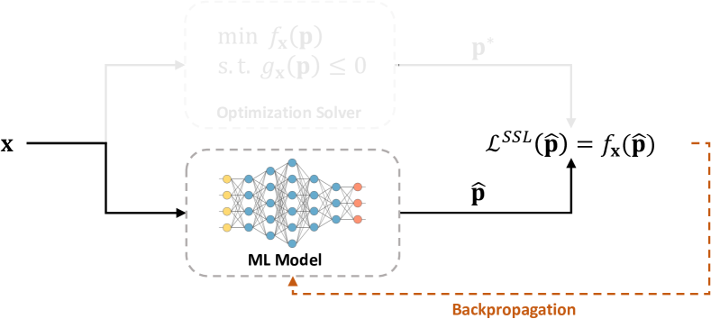
(b) Self-Supervised Learning: the loss function $\mathcal{L}^{SSL}$ measures the objective value of the prediction. No target $\mathbf{p}^{*}$ nor optimization solver is needed.

Figure 5: Illustration of supervised and self-supervised learning paradigms. When the ML model is not guaranteed to produce feasible solutions, the loss function $\mathcal{L}$ can be augmented with a constraint penalization term.

Consider a dataset of $N$ data points

$$\mathcal{D} =\Big{\{}\big{(}\mathbf{x}^{(1)},\mathbf{p}^{(1)}\big{)},...,\big{(}\mathbf{x}^{(N)},\mathbf{p}^{(N)}\big{)}\Big{\}},$$ (13)

where each data point corresponds to an instance of Problem (1) and its solution, i.e., $\mathbf{x}^{(i)}$ and $\mathbf{p}^{(i)}$ denote the input data and solution of instance $i\,{\in}\,\{1,...,N\}$, respectively. The training of the DNN $f_{\theta}$ can be formalized as the optimization problem

$$\theta^{*}=\operatorname*{arg-min}_{\theta}\quad \frac{1}{N}\sum_{i=1}^{N}\mathcal{L}\left(\hat{\mathbf{p}}^{(i)},\mathbf{p}^{(i)}\right),$$ (14)

where $\hat{\mathbf{p}}^{(i)}=f_{\theta^{*}}(\mathbf{x}^{(i)})$ is the prediction for instance $i$, and $\mathcal{L}$ denotes the loss function. The rest of this section describes the choice of loss function $\mathcal{L}$ for the SL and SSL settings.

V-A Supervised Learning

The supervised learning loss $\mathcal{L}^{\text{SL}}$ has the form

$$\mathcal{L}^{\text{SL}}(\hat{\mathbf{p}},\mathbf{p}) =\varphi^{\text{SL}}(\hat{\mathbf{p}},\mathbf{p})+\lambda\psi(\hat{\mathbf{p}}),$$ (15)

where $\varphi^{\text{SL}}(\hat{\mathbf{p}},\mathbf{p})$ penalizes the distance between the predicted and the target (ground truth) solutions, and $\psi(\hat{\mathbf{p}})$ penalizes constraint violations. The paper uses the Mean Absolute Error (MAE) on energy dispatch, i.e.,

$$\varphi^{\text{SL}}(\hat{\mathbf{p}},\mathbf{p}) =\frac{1}{|\mathcal{G}|}\|\hat{\mathbf{p}}-\mathbf{p}\|_{1}.$$ (16)

Note that other loss functions, e.g., Mean Squared Error (MSE), could be used instead. The term $\psi(\hat{\mathbf{p}})$ penalizes power balance violations and reserve shortages as follows:

$$\psi(\hat{\mathbf{p}})=M_{\text{pb}}|\mathbf{e}^{\top}\mathbf{d}-\mathbf{e}^{\top}\hat{\mathbf{p}}|+M_{\text{r}}\xi_{\text{r}}(\hat{\mathbf{p}}),$$ (17)

where $M_{\text{pb}}$ and $M_{\text{r}}$ are penalty coefficients, and $\xi_{\text{r}}$ denotes the reserve shortages, i.e.,

$$\xi_{\text{r}}(\hat{\mathbf{p}})=\max\big{\{}0,R-\sum_{g}\min(\bar{r}_{g},\bar{p}_{g}-\hat{p}_{g})\big{\}}.$$ (18)

The penalty term $\psi$ is set to zero for end-to-end feasible models. Finally, while thermal constraints are soft, preliminary experiments found that including thermal violations in the loss function yields more accurate models. This observation echoes the findings of multiple studies [6, 7, 15, 8, 17], namely, that penalizing constraint violations yields better accuracy and improves generalization. Indeed, the penalization of thermal violations acts as a regularizer in the loss function. Therefore, the final loss considered in the paper is

$$\mathcal{L}^{\text{SL}}(\hat{\mathbf{p}},\mathbf{p}) =\varphi^{\text{SL}}(\hat{\mathbf{p}},\mathbf{p})+\lambda\psi(\hat{\mathbf{p}})+\mu M_{\text{th}}\|\xi_{\text{th}}(\hat{\mathbf{p}})\|_{1},$$ (19)

where $\xi_{\text{th}}(\hat{\mathbf{p}})$ denotes thermal violations (Eq. (1g)).

V-B Self-supervised Learning

Self-supervised learning has been applied very recently to train optimization proxies [17, 32, 34]. The core aspect of SSL is that it does not require the labeled data $\mathbf{p}$, because it directly minimizes the objective function of the original problem. The self-supervised loss guides the training to imitate the solving of optimization instances using gradient-based algorithms, which makes it effective for optimization proxies.

The loss function $\mathcal{L}^{\text{SSL}}$ has the form

$$\mathcal{L}^{\text{SSL}}(\hat{\mathbf{p}}) =\varphi^{\text{SSL}}(\hat{\mathbf{p}})+\lambda\psi(\hat{\mathbf{p}}),$$ (20)

where $\psi(\hat{\mathbf{p}})$ is the same as Eq. (17), and

$$\varphi^{\text{SSL}}(\hat{\mathbf{p}}) =c(\hat{\mathbf{p}})+M_{\text{th}}\xi_{\text{th}}(\hat{\mathbf{p}})$$ (21)

is the objective value of the predicted solution. As mentioned above, note that $\mathcal{L}^{SLL}$ only depends on the predicted solution $\hat{\mathbf{p}}$, i.e., unlike the supervised learning loss $\mathcal{L}^{SL}$ (see Eq. (19)), it does not require any ground truth solution $\mathbf{p}$. Consequently, SSL does not require labeled data. This, in turn, eliminates the need to solve numerous instances offline.

Again, the constraint penalty term is zero when training end-to-end feasible models, because their output satisfies all hard constraints. Thereby, the self-supervised loss is very effective since the learning focuses on optimality.

For models without feasibility guarantees, the trade-off between optimality and feasibility typically makes the training very hard to stabilize for large-scale systems, which increases the learning difficulty. Thus, such models must take care to satisfy constraints to avoid spurious solutions. For instance, in the ED setting, simply minimizing total generation cost, without considering the power balance constraint (1b), yields the trivial solution $\mathbf{p}\,{=}\,\mathbf{0}$. This highlights the importance of ensuring feasibility, which is the core advantage of the proposed end-to-end feasible architecture.

VI Experiment settings

This section presents the numerical experiments used to assess E2ELR. The experiments are conducted on power grids with up to 30,000 buses and uses two variants of Problem 1 with and without reserve requirements. The section presents the data-generation methodology, the baseline ML architectures, performance metrics, and implementation details. Additional information is in [44].

VI-A Data Generation

TABLE I: Selected test cases from PGLib [45]

System	Ref	$|\mathcal{N}|$	$|\mathcal{E}|$	$|\mathcal{G}|$	${D_{\text{ref}}}^{\dagger}$	$\alpha_{\text{r}}$
ieee300	[46]	300	411	69	23.53	34.16%
pegase1k	[40]	1354	1991	260	73.06	19.82%
rte6470	[40]	6470	9005	761	96.59	14.25%
pegase9k	[40]	9241	16049	1445	312.35	4.70%
pegase13k	[40]	13659	20467	4092	381.43	1.32%
goc30k	[47]	30000	35393	3526	117.74	4.68%

^†Total active power demand in reference PGLib case, in GW.

Instances of Problem (1) are obtained by perturbing reference test cases from the PGLib [45] library (v21.07). Two categories of instances are generated: instances without any reserve requirements (ED), and instances with reserve requirements (ED-R). The instances are generated as follows. Denote by $\mathbf{d}^{\text{ref}}$ the nodal load vector from the reference PGLib case. ED instances are obtained by perturbing this reference load profile. Namely, for instance $i$, $\mathbf{d}^{(i)}\,{=}\,\gamma^{(i)}\times\eta^{(i)}\times\mathbf{d}^{\text{ref}}$, where $\gamma^{(i)}\,{\in}\,\mathbb{R}$ is a global scaling factor, $\eta\,{\in}\,\mathbb{R}^{|\mathcal{N}|}$ denotes load-level multiplicative white noise, and the multiplications are element-wise. For the case at hand, $\gamma$ is sampled from a uniform distribution $U[0.8,1.2]$, and, for each load, $\eta$ is sampled from a log-normal distribution with mean $1$ and standard deviation $5\%$.

ED-R instances are identical to the ED instances, except that reserve requirements are set to a non-zero value. The PGLib library does not include reserve information, therefore, the paper assumes $\bar{r}_{g}=\alpha_{\text{r}}\bar{p}_{g},\forall g\in\mathcal{G}$, where $\alpha_{\text{r}}=5\times\|\bar{\mathbf{p}}\|_{\infty}\times\|\bar{\mathbf{p}}\|_{1}^{-1}.$ This ensures that the total reserve capacity is 5 times larger than the largest generator in the system. Then, the reserve requirements of each instance is sampled uniformly between 100% and 200% of the size of the largest generator, thereby mimicking contingency reserve requirements used in industry.

Table I presents the systems used in the experiments. The table reports: the number of buses ($|\mathcal{N}|$), the number of branches ($|\mathcal{E}|$), the number of generators ($|\mathcal{G}|$), the total active power demand in the reference PGLib case ($D_{\text{ref}}$, in GW), and the value of $\alpha_{\text{r}}$ used to determine reserve capacities. The experiments consider test cases with up to 30,000 buses, significantly larger than almost all previous works. Large systems have a smaller value of $\alpha_{\text{r}}$ because they contain significantly more generators, whereas the size of the largest generator typically remains in the same order of magnitude. For every test case, $50,000$ instances are generated and solved using Gurobi. This dataset is then split into training, validation, and test sets which comprise $40000$, $5000$, and $5000$ instances.

VI-B Baseline Models

The proposed end-to-end learning and repair model (E2ELR) is evaluated against four architectures. First, a naive, fully-connected DNN model without any feasibility layer (DNN). This model only includes a sigmoid activation layer to enforce generation bounds (constraint (1e)). Second, a fully-connected DNN model with the DeepOPF architecture [7] (DeepOPF). It uses an equality completion to ensure the satisfaction of equality constraints; the output may violate inequality constraints. Third, a fully-connected DNN model with the DC3 architecture [17] (DC3). This architecture uses a fixed-step unrolled gradient descent to minimize constraint violations; it is however not guaranteed to reach zero violations. Note that the DC3 architecture requires a significant amount of hypertuning to achieve decent results. The last model is a fully-connected DNN model, combined with the LOOP-LC architecture from [39] (LOOP). The gauge mapping used in LOOP does not support the compact form of Eq. (12), therefore it is not included in the ED-R experiments. These baseline models are detailed in [44].

All baselines use a fully-connected DNN architecture, with the main difference being how feasibility is handled. Graph Neural Network (GNN) architectures are not considered in this work, as they were found to be numerically less stable and exhibited poorer performance than DNNs in preliminary experiments. Nevertheless, note that the proposed repair layers can also be used in conjunction with a GNN architecture.

VI-C Performance Metrics

The performance of each ML model is evaluated with respect to several metrics that measure both accuracy and computational efficiency. Given an instance $\mathbf{x}$ with optimal solution $\mathbf{p}^{*}$ and a predicted solution $\hat{\mathbf{p}}$, the optimality gap is defined as $\text{gap}=(\hat{Z}-Z^{*})\times|Z^{*}|^{-1},$ where $Z^{*}$ is the optimal value of the problem, and $\hat{Z}$ is the objective value of the prediction, plus a penalty for hard constraint violations, i.e.,

$$c(\hat{\mathbf{p}})+M_{\text{th}}\|\xi_{\text{th}}(\hat{\mathbf{p}})\|_{1}+M_{\text{pb}}|\mathbf{e}^{\top}(\hat{\mathbf{p}}-\mathbf{d})|+M_{\text{r}}\xi_{\text{r}}(\hat{\mathbf{p}}),$$ (22)

where $\xi_{\text{r}}(\hat{\mathbf{p}})$ is defined as in function (18). Penalizing hard constraint violations is necessary to ensure a fair comparison between models that output feasible solutions and those that do not. Because all considered models enforce constraints (1d)–(1f), they are not penalized in Eq. (22).

The paper uses realistic penalty prices, based on the values used by MISO in their operations [48, 49]. Namely, the thermal violation penalty price $M_{\text{th}}$ is set to $1500/MW. The power balance violation penalty $M_{\text{pb}}$ is set to $3500/MW, which corresponds to MISO’s value of lost load (VOLL). Finally, the reserve shortage penalty $M_{\text{r}}$ is set to $1100/MW, which is MISO’s reserve shortage price. The ability of optimization proxies to output feasible solution is measured via the proportion of feasible predictions, which is reported as a percentage over the test set. The paper uses an absolute tolerance of $10^{-4}$ p.u. to decide whether a constraint is violated; note that this is 100x larger than the default absolute tolerance of optimization solvers. The paper also reports the mean constraint violation of infeasible predictions.

The paper also evaluates the computational efficiency of each ML model and learning paradigm (SL and SSL), as well as that of the repair layers. Computational efficiency is measured by (i) the training time of ML models, including the data-generation time when applicable, and (ii) the inference time. Note that ML models evaluate batches of instances, therefore, inference times are reported per batch of 256 instances. The performance of the repair layers presented in Section IV is benchmarked against a standard euclidean projection solved with state-of-the-art optimization software.

Unless specified otherwise, average computing times are arithmetic means; other averages are shifted geometric means

$$\mu_{s}(x_{1},...,x_{n})=\exp\Big{(}\frac{1}{n}\sum_{i}\log(x_{i}+s)\Big{)}-s.$$

The paper uses a shift $s$ of 1% for optimality gaps, and 1p.u. for constraint violations.

VI-D Implementation Details

All optimization problems are formulated in Julia using JuMP [50], and solved with Gurobi 9.5 [51] with a single CPU thread and default parameter settings. All deep learning models are implemented using PyTorch [52] and trained using the Adam optimizer [53]. All models are hyperparameter tuned using a grid search, which is detailed in [44]. For each system, the best model is selected on the validation set and the performances on the test set are reported. During training, the learning rate is reduced by a factor of ten if the validation loss shows no improvement for a consecutive sequence of 10 epochs. In addition, training is stopped if the validation loss does not improve for consecutive 20 epochs. Experiments are conducted on dual Intel Xeon 6226@2.7GHz machines running Linux, on the PACE Phoenix cluster [54]. The training of ML models is performed on Tesla V100-PCIE GPUs with 16GBs HBM2 RAM.

VII Numerical Results

VII-A Optimality Gaps

Table II reports, for the ED and ED-R problems, the mean optimality gap of each ML model, under the SL and SSL learning modes. Bold entries denote the best-performing method. Recall that LOOP is not included in ED-R experiments. E2ELR systematically outperforms all other baselines across all settings. This stems from two reasons. First, DNN, DeepOPF and DC3 exhibit violations of the power balance constraint (1b), which yields high penalties and therefore large optimality gaps. Statistics on power balance violations for DNN, DeepOPF and DC3 are reported in Table III. Second, LOOP’s poor performance, despite not violating any hard constraint, is because the non-convex gauge mapping used inside the model has an adverse impact on training. Indeed, after a few epochs of training, LOOP gets stuck in a local optimum.

TABLE II: Mean optimality Gap (%) on test set

		ED					ED-R
Loss	System	DNN	E2ELR	DeepOPF	DC3	LOOP	DNN	E2ELR	DeepOPF	DC3
SL	ieee300	69.55	1.42	2.81	3.03	38.93	75.06	1.52	2.80	2.94
	pegase1k	48.77	0.74	7.78	2.80	32.53	47.84	0.74	7.50	2.97
	rte6470	55.13	1.35	28.23	3.68	50.21	70.57	1.82	46.66	3.49
	pegase9k	76.06	0.38	33.20	1.25	33.78	81.19	0.38	30.84	1.29
	pegase13k	71.14	0.29	64.93	1.79	52.94	76.32	0.28	69.23	1.81
	goc30k	194.13	0.46	55.91	2.75	36.49	136.25	0.45	41.34	2.35
SSL	ieee300	35.66	0.74	2.23	2.51	37.78	45.56	0.78	2.82	2.80
	pegase1k	62.07	0.63	10.83	2.57	32.20	64.69	0.68	9.83	2.61
	rte6470	40.73	1.30	42.28	2.82	50.20	55.16	1.68	48.57	3.04
	pegase9k	43.68	0.32	34.33	0.82	33.76	44.74	0.29	42.06	0.93
	pegase13k	57.58	0.21	60.12	0.84	52.93	61.28	0.19	65.38	0.91
	goc30k	108.91	0.39	8.39	0.72	36.73	93.91	0.33	9.47	0.71

TABLE III: Power balance constraint violation statistics

		ED						ED-R
		DNN		DeepOPF		DC3		DNN		DeepOPF		DC3
Loss	System	%feas	viol	%feas	viol	%feas	viol	%feas	viol	%feas	viol	%feas	viol
SL	ieee300	0%	0.50	100%	0.00	100%	0.00	0%	0.70	100%	0.06	100%	0.25
	pegase1k	0%	1.82	71%	1.35	65%	0.04	0%	1.90	70%	1.19	65%	0.08
	rte6470	0%	2.08	1%	1.94	9%	0.03	0%	2.26	1%	2.81	7%	0.01
	pegase9k	0%	6.25	3%	6.38	29%	0.00	0%	5.91	3%	5.99	29%	0.00
	pegase13k	0%	6.63	1%	7.08	23%	0.00	0%	7.79	1%	7.46	22%	0.00
	goc30k	0%	3.81	45%	1.70	57%	0.03	0%	2.31	54%	1.54	69%	0.00
SSL	ieee300	0%	0.58	100%	0.00	100%	0.16	0%	0.73	100%	0.56	100%	0.29
	pegase1k	0%	2.42	63%	2.56	63%	0.03	0%	2.30	63%	1.81	39%	0.05
	rte6470	0%	1.90	1%	2.64	6%	0.11	0%	2.72	1%	2.51	5%	0.01
	pegase9k	0%	7.22	3%	5.46	27%	0.05	0%	7.00	3%	7.87	25%	0.08
	pegase13k	0%	6.41	1%	7.19	19%	0.01	0%	6.82	1%	7.83	20%	0.01
	goc30k	0%	3.18	55%	1.24	52%	0.01	0%	2.61	49%	1.20	62%	0.02

^†with 200 gradient steps. ^∗geometric mean of non-zero violations, in p.u.

E2ELR, when trained in a self-supervised mode, achieves the best performance. This is because SSL directly minimizes the true objective function, rather than the surrogate supervised loss. With the exception of rte6470, the performance of E2ELR improves as the size of the system increases, with the lowest optimality gaps achieved on pegase13k, which has the most generators. Note that rte6470is a real system from the French transmission grid: it is more congested than other test cases, and therefore harder to learn.

VII-B Computing Times

Tables IV and V report the sampling and training times for ED and ED-R, respectively. Each table reports the total time for data-generation, which corresponds to the total solving time of Gurobi on a single thread. There is no labeling time for self-supervised models. While training times for SL and SSL are comparable, for a given architecture, the latter does not incur any labeling time. The training time of DC3 is significantly higher than other baselines because of its unrolled gradient steps. These results demonstrate that ML models can be trained efficiently on large-scale systems. Indeed, the self-supervised E2ELR needs less than an hour of total computing time to achieve optimality gaps under $0.5\%$ for systems with thousands of buses.

TABLE IV: Sampling and training time comparison (ED)

Loss	System	Sample	DNN	E2ELR	DeepOPF	DC3	LOOP
SL	ieee300	[mode=text] 0.2	[mode=text] 7	[mode=text]37	[mode=text]31	[mode=text]121	[mode=text] 33
	pegase1k	[mode=text] 0.7	[mode=text] 8	[mode=text]14	[mode=text] 6	[mode=text] 41	[mode=text] 19
	rte6470	[mode=text] 5.1	[mode=text]11	[mode=text]30	[mode=text]13	[mode=text] 73	[mode=text] 18
	pegase9k	[mode=text]12.7	[mode=text]15	[mode=text]24	[mode=text]22	[mode=text]123	[mode=text] 25
	pegase13k	[mode=text]20.6	[mode=text]14	[mode=text]19	[mode=text]14	[mode=text]126	[mode=text] 19
	goc30k	[mode=text]63.4	[mode=text]25	[mode=text]20	[mode=text]41	[mode=text]108	[mode=text]127
SSL	ieee300	–	[mode=text]15	[mode=text]27	[mode=text]38	[mode=text]102	[mode=text]27
	pegase1k	–	[mode=text] 8	[mode=text]15	[mode=text]11	[mode=text] 46	[mode=text]14
	rte6470	–	[mode=text] 9	[mode=text]17	[mode=text]10	[mode=text] 42	[mode=text]15
	pegase9k	–	[mode=text]18	[mode=text]20	[mode=text]17	[mode=text]100	[mode=text]29
	pegase13k	–	[mode=text]17	[mode=text]18	[mode=text]14	[mode=text]125	[mode=text]15
	goc30k	–	[mode=text]38	[mode=text]45	[mode=text]51	[mode=text]105	[mode=text]60

Sampling (training) times are for 1 CPU (1 GPU). Excludes hypertuning.

TABLE V: Sampling and training time comparison (ED-R)

Loss	System	Sample	DNN	E2ELR	DeepOPF	DC3
SL	ieee300	[mode=text] 0.2	[mode=text]12	[mode=text]43	[mode=text]43	[mode=text]115
	pegase1k	[mode=text] 0.8	[mode=text]14	[mode=text]19	[mode=text]19	[mode=text]53
	rte6470	[mode=text] 4.6	[mode=text]14	[mode=text]19	[mode=text]19	[mode=text]71
	pegase9k	[mode=text]14.0	[mode=text]15	[mode=text]22	[mode=text]22	[mode=text]123
	pegase13k	[mode=text]22.7	[mode=text]16	[mode=text]27	[mode=text]27	[mode=text]126
	goc30k	[mode=text]65.9	[mode=text]32	[mode=text]39	[mode=text]38	[mode=text]129
SSL	ieee300	–	[mode=text]21	[mode=text]37	[mode=text]37	[mode=text]131
	pegase1k	–	[mode=text] 6	[mode=text]19	[mode=text]19	[mode=text] 67
	rte6470	–	[mode=text]12	[mode=text]21	[mode=text]21	[mode=text] 71
	pegase9k	–	[mode=text]20	[mode=text]24	[mode=text]24	[mode=text]123
	pegase13k	–	[mode=text]13	[mode=text]22	[mode=text]22	[mode=text]125
	goc30k	–	[mode=text]52	[mode=text]53	[mode=text]53	[mode=text]128

Sampling (training) times are for 1 CPU (1 GPU). Excludes hypertuning.

Tables VI and VII report, for ED and ED-R, respectively, the average solving time using Gurobi (GRB) and average inference times of ML methods. Recall that the Gurobi’s solving times are for a single instance solved on a single CPU core, whereas the ML inference times are reported for a batch of 256 instances on a GPU. Also note that the number of gradient steps used by DC3 to recover feasibility is set to 200 for inference (compared to 50 for training).

On systems with more than 6,000 buses, DC3 is typically 10–30 times slower than other baselines, again due to its unrolled gradient steps. In contrast, DNN, DeepOPF, E2ELR, and LOOP all require in the order of 5–10 milliseconds to evaluate a batch of 256 instances. For the largest systems, this represents about 25,000 instances per second, on a single GPU. Solving the same volume of instances with Gurobi would require more than a day on a single CPU. Getting this time down to the order of seconds, thereby matching the speed of ML proxies, would require thousands of CPUs, which comes at high financial and environmental costs.

TABLE VI: Solving and inference time comparison (ED)

Loss	System	DNN	E2ELR	DeepOPF	DC3†	LOOP	GRB∗
SL	ieee300	[mode=text]3.4	[mode=text]4.5	[mode=text]4.8	[mode=text]15.4	[mode=text]5.3	[mode=text]12.1
	pegase1k	[mode=text]4.1	[mode=text]5.3	[mode=text]4.3	[mode=text]18.3	[mode=text]5.9	[mode=text]51.5
	rte6470	[mode=text]5.1	[mode=text]6.6	[mode=text]5.4	[mode=text]35.3	[mode=text]7.1	[mode=text]364.4
	pegase9k	[mode=text]6.0	[mode=text]7.3	[mode=text]6.2	[mode=text]91.5	[mode=text]8.2	[mode=text]913.5
	pegase13k	[mode=text]7.3	[mode=text]8.3	[mode=text]8.7	[mode=text]523.6	[mode=text]13.9	[mode=text]1481.3
	goc30k	[mode=text]9.5	[mode=text]10.0	[mode=text]9.3	[mode=text]443.0	[mode=text]14.4	[mode=text]4566.9
SSL	ieee300	[mode=text]3.4	[mode=text]6.0	[mode=text]3.7	[mode=text]15.1	[mode=text]5.2	[mode=text]12.1
	pegase1k	[mode=text]4.0	[mode=text]5.3	[mode=text]4.3	[mode=text]18.4	[mode=text]5.8	[mode=text]51.5
	rte6470	[mode=text]5.9	[mode=text]6.5	[mode=text]6.3	[mode=text]36.7	[mode=text]9.5	[mode=text]364.4
	pegase9k	[mode=text]6.1	[mode=text]7.0	[mode=text]6.3	[mode=text]93.2	[mode=text]10.3	[mode=text]913.5
	pegase13k	[mode=text]7.1	[mode=text]8.2	[mode=text]7.2	[mode=text]561.2	[mode=text]12.8	[mode=text]1481.3
	goc30k	[mode=text]10.9	[mode=text]11.7	[mode=text]9.4	[mode=text]444.2	[mode=text]21.7	[mode=text]4566.9

^†with 200 gradient steps. ^∗solution time per instance (single thread).
All ML inference times are for a batch of 256 instances.

TABLE VII: Solving and inference time comparison (ED-R)

Loss	System	DNN	E2ELR	DeepOPF	DC3†	GRB∗
SL	ieee300	[mode=text] 3.9	[mode=text] 6.5	[mode=text]4.6	[mode=text] 16.5	[mode=text] 12.6
	pegase1k	[mode=text] 4.5	[mode=text] 6.0	[mode=text]4.8	[mode=text] 18.9	[mode=text] 56.5
	rte6470	[mode=text] 5.7	[mode=text] 10.4	[mode=text]6.2	[mode=text] 36.1	[mode=text] 333.6
	pegase9k	[mode=text] 6.3	[mode=text] 7.7	[mode=text]6.7	[mode=text] 91.6	[mode=text]1008.0
	pegase13k	[mode=text] 8.3	[mode=text] 10.7	[mode=text]8.8	[mode=text] 531.2	[mode=text]1632.7
	goc30k	[mode=text] 9.3	[mode=text] 11.1	[mode=text]10.6	[mode=text] 438.7	[mode=text]4745.7
SSL	ieee300	[mode=text] 3.9	[mode=text] 7.6	[mode=text]4.4	[mode=text] 17.6	[mode=text] 12.6
	pegase1k	[mode=text] 4.4	[mode=text] 5.9	[mode=text]4.7	[mode=text] 19.1	[mode=text] 56.5
	rte6470	[mode=text] 6.4	[mode=text] 10.5	[mode=text]6.7	[mode=text] 37.3	[mode=text] 333.6
	pegase9k	[mode=text] 7.1	[mode=text] 8.3	[mode=text]7.2	[mode=text] 92.9	[mode=text]1008.0
	pegase13k	[mode=text] 7.8	[mode=text] 8.9	[mode=text]7.9	[mode=text] 522.4	[mode=text]1632.7
	goc30k	[mode=text] 10.2	[mode=text] 12.4	[mode=text]10.3	[mode=text] 435.8	[mode=text]4745.7

^†with 200 gradient steps. ^∗solution time per instance (single thread).
All ML inference times are for a batch of 256 instances.

VII-C Benefits of End-to-End Training

TABLE VIII: Comparison of optimality gaps (%) with and without feasibility restoration (ED)

			DNN			DeepOPF			DC3
Loss	System	E2ELR	–	FL	EP	–	FL	EP	–	FL	EP
SL	ieee300	1.42	69.55	36.33	36.37	2.81	2.81	2.81	3.03	3.03	3.03
	pegase1k	0.74	48.77	3.98	3.94	7.78	5.24	5.28	2.80	2.44	2.44
	rte6470	1.35	55.13	21.28	21.41	28.23	1.89	1.89	3.68	3.36	3.36
	pegase9k	0.38	76.06	34.61	34.65	33.20	1.94	1.99	1.25	1.24	1.24
	pegase13k	0.29	71.14	32.70	32.72	64.93	23.36	23.36	1.79	1.79	1.79
	goc30k	0.46	194.13	57.53	57.41	55.91	30.19	30.16	2.75	2.45	2.45
SSL	ieee300	0.74	35.66	3.82	3.73	2.23	2.23	2.23	2.51	2.51	2.51
	pegase1k	0.63	62.07	3.24	3.25	10.83	3.21	3.18	2.57	2.35	2.35
	rte6470	1.30	40.73	11.52	11.47	42.28	5.38	5.37	2.82	2.10	2.09
	pegase9k	0.32	43.68	3.20	3.22	34.33	4.73	4.74	0.82	0.64	0.64
	pegase13k	0.21	57.58	20.59	20.59	60.12	18.85	18.84	0.84	0.81	0.81
	goc30k	0.39	108.91	7.89	7.89	8.39	3.06	3.06	0.72	0.62	0.62

TABLE IX: Comparison of optimality gaps (%) with and without feasibility restoration (ED-R)

			DNN			DeepOPF			DC3
Loss	System	E2ELR	–	FL	EP	–	FL	EP	–	FL	EP
SL	ieee300	1.52	75.06	30.47	30.49	2.80	2.80	2.80	2.94	2.94	2.94
	pegase1k	0.74	47.84	2.52	2.50	7.50	4.79	4.79	2.97	2.34	2.34
	rte6470	1.82	70.57	30.20	29.90	46.66	2.63	2.51	3.49	3.32	3.29
	pegase9k	0.38	81.19	41.34	41.40	30.84	1.90	1.92	1.29	1.29	1.29
	pegase13k	0.28	76.32	30.00	30.02	69.23	25.09	25.09	1.81	1.81	1.81
	goc30k	0.45	136.25	53.34	53.41	41.34	22.53	22.43	2.35	2.31	2.31
SSL	ieee300	0.78	45.56	4.50	4.34	2.82	2.79	2.79	2.80	2.78	2.78
	pegase1k	0.68	64.69	4.56	4.44	9.83	3.97	3.95	2.61	1.87	1.87
	rte6470	1.68	55.16	9.76	9.43	48.57	8.79	8.53	3.04	2.75	2.70
	pegase9k	0.29	44.74	4.33	4.33	42.06	2.28	2.30	0.93	0.66	0.66
	pegase13k	0.19	61.28	21.35	21.32	65.38	19.64	19.64	0.91	0.89	0.89
	goc30k	0.33	93.91	10.00	9.98	9.47	2.58	2.58	0.71	0.64	0.64

Tables VIII and IX further demonstrate the benefits of training end-to-end feasible models: they report, for ED and ED-R problems, the optimality gaps achieved by DNN, DeepOPF and DC3 after applying a repair step at inference time. Two repair mechanisms are compared: the proposed Repair Layers (RL) and a Euclidean Projection (EP). The tables also report the mean gap achieved by E2ELR as a reference baseline. The results can be summarized as follows. First, the additional feasibility restoration improves the quality of the initial prediction. This is especially true for DNN and DeepOPF, which exhibited the largest constraint violations (see Table III): optimality gaps are improved by a factor 2–20, but remain very high nonetheless. Second, the two repair mechanisms yield similar optimality gaps. For DC3, there is virtually no difference between RL and EP. Third, across all experiments, even after feasibility restoration, E2ELR remains the best-performing model, with optimality gaps 2–6x smaller than DC3. Table X compares the computing times of the feasibility restoration using either the repair layers (RL) or the euclidean projection (EP). The latter is solved as a quadratic program with Gurobi. All benchmarks are conducted in Julia on a single thread, using the BenchmarkTools utility [55], and median times are reported. The results of Table X show that evaluating the proposed repair layers is three orders of magnitude faster than solving the euclidean projection problem.

TABLE X: Computing time of feasibility restoration using feasibility layers (FL) and Euclidean projection (EP).

Problem	System	RL	EP	Speedup
ED	ieee300	[mode=text] 0.13	[mode=text] 0.45	3439x
	pegase1k	[mode=text] 0.55	[mode=text] 1.41	2572x
	rte6470	[mode=text] 1.40	[mode=text] 3.75	2686x
	pegase9k	[mode=text] 2.37	[mode=text] 6.90	2911x
	pegase13k	[mode=text] 6.42	[mode=text] 20.71	3227x
	goc30k	[mode=text] 5.67	[mode=text] 17.87	3155x
ED-R	ieee300	[mode=text] 1.06	[mode=text] 1.00	939x
	pegase1k	[mode=text] 4.58	[mode=text] 3.42	748x
	rte6470	[mode=text] 10.46	[mode=text] 10.19	974x
	pegase9k	[mode=text] 20.14	[mode=text] 18.38	913x
	pegase13k	[mode=text] 42.67	[mode=text] 60.73	1423x
	goc30k	[mode=text] 39.80	[mode=text] 49.17	1236x

Median computing times as measured by BenchmarkTools

VIII Conclusion

The paper proposed a new End-to-End Learning and Repair (E2ELR) architecture for training optimization proxies for economic dispatch problems. E2ELR combines deep learning with closed-form, differential repair layers, thereby integrating prediction and feasibility restoration in an end-to-end fashion. The E2ELR architecture can be trained with self-supervised learning, removing the need for labeled data and the solving of numerous optimization problems offline. The paper conducted extensive numerical experiments on the ecocomic dispatch of large-scale, industry-size power grids with tens of thousands of buses. It also presented the first study that considers reserve requirements in the context of optimization proxies, reducing the gap between academic and industry formulations. The results demonstrate that the combination of E2ELR and self-supervised learning achieves state-of-the-art performance, with optimality gaps that outperform other baselines by at least an order of magnitude. Future research will investigate security-constrained economic dispatch (SCED) formulations, and the extension of repair layers to thermal constraints, multi-period settings and the nonlinear, non-convex AC-OPF.

-A Proofs

-A1 Proof of Theorem 1

Let $\mathbf{\tilde{p}}\,{=}\,\mathcal{P}(\mathbf{p})$, and assume $\mathbf{e}^{\top}\mathbf{p}\,{<}\,D$. It is immediate that $\eta^{\uparrow}\,{\in}\,[0,1]$, i.e., $\mathbf{\tilde{p}}$ is a convex combination of $\mathbf{p}$ and $\mathbf{\bar{p}}$. Thus, $\mathbf{\tilde{p}}\in\mathcal{H}$. Then,

$$\mathbf{e}^{\top}\mathbf{\tilde{p}} =(1-\eta^{\uparrow})\mathbf{e}^{\top}\mathbf{p}+\eta^{\uparrow}\mathbf{e}^{\top}\bar{\mathbf{p}}$$

$$=\eta^{\uparrow}(\mathbf{e}^{\top}\bar{\mathbf{p}}-\mathbf{e}^{\top}\mathbf{p})+\mathbf{e}^{\top}\mathbf{p}$$

$$=\frac{D-\mathbf{e}^{\top}\mathbf{p}}{\mathbf{e}^{\top}\mathbf{\bar{p}}-\mathbf{e}^{\top}\mathbf{p}}(\mathbf{e}^{\top}\bar{\mathbf{p}}-\mathbf{e}^{\top}\mathbf{p})+\mathbf{e}^{\top}\mathbf{p}$$

$$=D-\mathbf{e}^{\top}\mathbf{p}+\mathbf{e}^{\top}\mathbf{p}=D.$$

Thus, $\mathbf{\tilde{p}}$ satisfies the power balance and $\mathbf{\tilde{p}}\in\mathcal{S}_{D}$. Similarly, assume $\mathbf{e}^{\top}\mathbf{p}\geq D$. Then

$$\mathbf{e}^{\top}\mathbf{\tilde{p}} =(1-\eta^{\downarrow})\mathbf{e}^{\top}\mathbf{p}+\eta^{\downarrow}\mathbf{e}^{\top}\mathbf{0}$$

$$=(1-\frac{\mathbf{e}^{\top}\mathbf{p}-D}{\mathbf{e}^{\top}\mathbf{p}})\mathbf{e}^{\top}\mathbf{p}=D,$$

which concludes the proof. ∎

-A2 Proof of Theorem 2

Let $\mathbf{p}$ be the initial prediction, and let $\mathbf{\tilde{p}}=\mathcal{R}(\mathbf{p})$. First, the bound constraints $\mathbf{0}\,{\leq}\,\mathbf{p}\,{\leq}\,\mathbf{\bar{p}}$ are satisfied because $\mathbf{\tilde{p}}$ is a convex combination of $\mathbf{p}$ and $\mathbf{\bar{p}}-\mathbf{\bar{r}}$, both of which satisfy bound constraints.

Second, we show that $\mathbf{e}^{\top}\mathbf{p}=D$. Indeed, we have

$$\sum_{g}\tilde{p}_{g} =\sum_{g\in G^{\uparrow}}\tilde{p}_{g}+\sum_{g\in G^{\downarrow}}\tilde{p}_{g}$$ (23)

This yields

$$\sum_{g\in G^{\uparrow}}\tilde{p}_{g} =\sum_{g\in G^{\uparrow}}(1-\alpha^{\uparrow})p_{g}+\alpha^{\uparrow}(\bar{p}_{g}-\bar{r}_{g})$$

$$=\sum_{g\in G^{\uparrow}}p_{g}+\alpha^{\uparrow}\sum_{g\in G^{\uparrow}}(\bar{p}_{g}-\bar{r}_{g}-p_{g})$$

$$=\sum_{g\in\uparrow}p_{g}+\alpha^{\uparrow}\Delta^{\uparrow}$$

$$=\sum_{g\in G^{\uparrow}}p_{g}+\Delta$$

$$\sum_{g\in G^{\downarrow}}\tilde{p}_{g} =\sum_{g\in G^{\downarrow}}(1-\alpha^{\downarrow})p_{g}+\alpha^{\downarrow}(\bar{p}_{g}-\bar{r}_{g})$$

$$=\sum_{g\in G^{\downarrow}}p_{g}+\alpha^{\downarrow}\sum_{g\in G^{\downarrow}}(\bar{p}_{g}-\bar{r}_{g}-p_{g})$$

$$=\sum_{g\in G^{\downarrow}}p_{g}-\alpha^{\downarrow}\Delta^{\downarrow}$$

$$=\sum_{g\in G^{\downarrow}}p_{g}-\Delta$$

Summing the two terms yields $\mathbf{e}^{\top}\mathbf{p}+\Delta-\Delta=D$.

Finally, we show that Algorithm 1 provides a feasible point iff DCOPF is feasible. If $\mathbf{\tilde{p}}$ is reserve feasible, then DCOPF is trivially feasible.

Assume $\mathbf{\tilde{p}}$ is infeasible, i.e., $\sum_{g}\min(\bar{r}_{g},\bar{p}-\tilde{p}_{g})<R$. Note that if $\Delta=\Delta_{R}$ in Algorithm 1, then $\mathbf{\tilde{p}}$ is feasible, so we must have $\Delta^{\uparrow}<\Delta_{R}$ or $\Delta^{\downarrow}<\Delta_{R}$.

Assume the former holds, i.e., $\Delta^{\uparrow}<\Delta_{R},\Delta_{\downarrow}$. In other words:

$$\sum_{g\in G^{\uparrow}}\bar{p}_{g}-\bar{r}_{g}-p_{g}<R-\sum_{g\in G^{\uparrow}}\bar{r}_{g}-\sum_{g\in G^{\downarrow}}\bar{p}_{g}-p_{g}$$

$$\sum_{g\in G^{\uparrow}}(\bar{p}_{g}-\bar{r}_{g}-p_{g}+\bar{r}_{g})<R-\sum_{g\in G^{\downarrow}}\bar{p}_{g}-p_{g}$$

$$\sum_{g\in G^{\uparrow}}(\bar{p}_{g}-p_{g})<R-\sum_{g\in G^{\downarrow}}\bar{p}_{g}-p_{g}$$

$$\sum_{g\in G^{\uparrow}}\bar{p}_{g}+\sum_{g\in G^{\downarrow}}\bar{p}_{g}<R-\sum_{g}p_{g}$$

$$\sum_{g}\bar{p}_{g}<R-D$$

Summing constraints (1d) and (1b), we obtain

$$\sum_{g}r_{g}\leq(\sum_{g}\bar{p}_{g})-D<R$$

hence DCOPF is infeasible. The proof for $\Delta^{\downarrow}<\Delta_{R}$ is similar. ∎

-B Details of the baseline models

Both DC3 [17] and LOOP-LC [39] follow the steps of neural network prediction, inequality correction, and equality completion. First, the decision variables are divided into two groups: $|\mathcal{G}|-N_{eq}$ independent decision variables and $N_{eq}$ dependent decision variables, where $N_{eq}$ indicates the number of equality constraints. In the PTDF formulation of DC-OPF, the only equality constraint is the power balance constraint (1b), and thus $N_{eq}=1$. Therefore, given the dispatches of the independent generator are predicted, the dispatch of the dependent generator can be recovered by

$$p_{1}=D-\sum_{g\in{\mathcal{G}}\setminus 1}p_{g}.$$ (24)

DC3 and LOOP-LC differ in their inequality corrections.

DC3

Given the input load profile $\mathbf{l}\in\mathbb{R}^{|\mathcal{L}|}$, the neural network outputs $\mathbf{z}\in[0,1]^{|\mathcal{G}|-1}$. This is achieved by applying a sigmoid function to the final layer of the network. Then the capacity constraints (1d) are enforced by:

$$p_{g}=z_{g}*\bar{p}_{g},\;\;\forall g\in\mathcal{G}\setminus 1.$$

In the inequality correction steps, DC3 minimizes the constraint violation by unrolling gradient descent with a fixed number of iterations $T$. Denote the constraint violation

$$g(\mathbf{p})=\sum_{g\in\mathcal{G}}\max(p_{g}-\bar{p}_{g},0)+\max(R-\sum_{g\in\mathcal{G}}r_{g},0),$$

where $r_{g}=\min\{\bar{r}_{g},\bar{p}_{g}-p_{g}\}$ and $p_{1}=D-\sum_{g\in{\mathcal{G}}\setminus 1}p_{g}$. The dispatch is updated using:

$$\mathbf{p}^{t}=\mathbf{p}^{t-1}-\rho*\nabla_{\mathbf{p}}\|g(\mathbf{p}^{t-1})\|^{2}_{2},$$

where $\mathbf{p}^{0}$ is the output of the neural network. In the experiment, the step size $\rho$ is set as $1e-4$ and the total iteration $T$ is set as $50$ when training and $200$ when testing. The longer testing $T$ is suggested in [17] to mitigate the constraint violation of DC3 predictions.

LOOP-LC

Similar to DC3, the neural network maps the load profile $\mathbf{l}\in\mathbb{R}^{|\mathcal{L}|}$ to $\mathbf{z}\in[0,1]^{|\mathcal{G}|-1}$ by applying a sigmoid function at the end. In the inequality correction step, LOOP-LC uses gauge function mapping $\mathbf{z}$ in the $l_{\infty}$ norm ball to the dispatches in the feasible region. The gauge mapping needs an interior point to shift the domain. The work in [39] proposes an interior point finder by solving an optimization, which could be computationally expensive. Instead, the experiments exploit the proposed feasibility restoration layers to find the interior point effectively. Specifically, the interior point finder consists of two steps. First, the optimal dispatches of the nominal case $\mathbf{p}^{n}$ are obtained by solving the instance with the nominal active power demand as the input, where the upper bounds $\bar{p}_{g}$ in constraints (1d) and (1e) are scaled with $\beta\in(0,1)$: $\mathbf{p}+\mathbf{r}\leq\beta\mathbf{\bar{p}}$ and $\mathbf{0}\leq\mathbf{p}\leq\beta\mathbf{\bar{p}}$, where the $\beta$ is set as $0.8$ in the experiments. The scaling aims at providing a more interior point such that the gauge mapping is more smooth. However, the $\mathbf{p}^{n}$ may not be feasible when changing the input load profile $\mathbf{l}$. To obtain the feasible solution, the proposed feasibility layers are used to convert $\mathbf{p}^{n}$ to an interior point.

-C Hyperparameter Tuning

For each test case and method, the number of instances in the training and test minibatch are set to 64 and 256, respectively. For all deep learning models, a batch normalization layer [56] and a dropout layer [57] with a dropout rate $0.2$ are appended after each dense layer except the last one. The number of layers $l$ is selected from $\{3,4,5\}$ and the hidden dimension $hd$ of the dense layers is selected from $\{128,256\}$.

The penalty coefficients $\lambda$ of the constraint violation in the loss function 19 and 20 are selected from $\{1,0.1\}$ for self-supervised learning and selected from $\{1e-3,1e-4,1e-5\}$ for supervised learning. For the models with feasibility guarantees such as DNN-F and LOOP, the $\lambda$ is set as 0 for self-supervised learning. $\mu$ is set to be equal to $\lambda$ for supervised learning. For DC3 model, the unrolled iteration is set as $50$ iterations in training and $200$ iterations in testing. The gradient step size is set as $1e-4$, where a larger step size results in numerical issues.

The models are trained with Adam optimizer [53] with an initial learning rate is set as $1e-2$ and weight delay $1e-6$. The learning rate is decayed by 0.1 when the validation loss does not improve for consecutive 10 epochs and the training early stops if the validation loss does not decrease for consecutive 20 epochs. The maximum training time is set as 150 minutes.

References

- [1] MISO, “Energy and operating reserve markets,” 2022, Business Practices Manual Energy and Operating Reserve Markets.
- [2] Midcontinent ISO, “MISO’s response to the reliability imperative,” 1 2023. [Online]. Available: https://cdn.misoenergy.org/MISO\%20Response\%20to\%20the\%20Reliability\%20Imperative504018.pdf
- [3] O. Stover, P. Karve, and S. Mahadevan, “Reliability and risk metrics to assess operational adequacy and flexibility of power grids,” Reliability Engineering & System Safety, vol. 231, p. 109018, 2023.
- [4] O. Stover, P. Karve, S. Mahadevan, W. Chen, H. Zhao, M. Tanneau, and P. V. Hentenryck, “Just-In-Time Learning for Operational Risk Assessment in Power Grids,” 2022.
- [5] W. Chen, S. Park, M. Tanneau, and P. Van Hentenryck, “Learning Optimization Proxies for Large-Scale Security-Constrained Economic Dispatch,” Electric Power Systems Research, vol. 213, p. 108566, 2022.
- [6] Y. Ng, S. Misra, L. A. Roald, and S. Backhaus, “Statistical learning for dc optimal power flow,” in 2018 Power Systems Computation Conference (PSCC), 2018, pp. 1–7.
- [7] X. Pan, T. Zhao, M. Chen, and S. Zhang, “DeepOPF: A Deep Neural Network Approach for Security-Constrained DC OPF,” IEEE Transactions on Power Systems, vol. 36, no. 3, pp. 1725–1735, 2020.
- [8] R. Nellikkath and S. Chatzivasileiadis, “Physics-informed neural networks for minimising worst-case violations in dc optimal power flow,” in IEEE International Conference on Communications, Control, and Computing Technologies for Smart Grids (SmartGridComm), 2021, pp. 419–424.
- [9] T. Zhao, X. Pan, M. Chen, and S. Low, “Ensuring DNN Solution Feasibility for Optimization Problems with Linear Constraints,” in The Eleventh International Conference on Learning Representations, 2023.
- [10] A. Stratigakos, S. Pineda, J. M. Morales, and G. Kariniotakis, “Interpretable Machine Learning for DC Optimal Power Flow with Feasibility Guarantees,” Mar. 2023, working paper or preprint. [Online]. Available: https://hal.science/hal-04038380
- [11] R. Ferrando, L. Pagnier, R. Mieth, Z. Liang, Y. Dvorkin, D. Bienstock, and M. Chertkov, “A Physics-Informed Machine Learning for Electricity Markets: A NYISO Case Study,” 2023. [Online]. Available: https://doi.org/10.48550/arXiv.2304.00062
- [12] N. Guha, Z. Wang, M. Wytock, and A. Majumdar, “Machine Learning for AC Optimal Power Flow,” 2019.
- [13] A. S. Zamzam and K. Baker, “Learning Optimal Solutions for Extremely Fast AC Optimal Power Flow,” in 2020 IEEE International Conference on Communications, Control, and Computing Technologies for Smart Grids (SmartGridComm), 2020, pp. 1–6.
- [14] D. Owerko, F. Gama, and A. Ribeiro, “Optimal Power Flow Using Graph Neural Networks,” in ICASSP 2020 - 2020 IEEE International Conference on Acoustics, Speech and Signal Processing (ICASSP), 2020, pp. 5930–5934.
- [15] F. Fioretto, T. W. Mak, and P. Van Hentenryck, “Predicting AC Optimal Power Flows: Combining deep learning and lagrangian dual methods,” in Proceedings of the AAAI conference on artificial intelligence, vol. 34, no. 01, 2020, pp. 630–637.
- [16] M. Chatzos, T. W. Mak, and P. Van Hentenryck, “Spatial network decomposition for fast and scalable AC-OPF learning,” IEEE Transactions on Power Systems, vol. 37, no. 4, pp. 2601–2612, 2021.
- [17] P. Donti, D. Rolnick, and J. Z. Kolter, “DC3: A learning method for optimization with hard constraints,” in International Conference on Learning Representations, 2021.
- [18] R. Nellikkath and S. Chatzivasileiadis, “Physics-informed neural networks for ac optimal power flow,” Electric Power Systems Research, vol. 212, p. 108412, 2022.
- [19] X. Pan, M. Chen, T. Zhao, and S. H. Low, “DeepOPF: A Feasibility-Optimized Deep Neural Network Approach for AC Optimal Power Flow Problems,” IEEE Systems Journal, vol. 17, no. 1, pp. 673–683, 2023.
- [20] X. Pan, W. Huang, M. Chen, and S. H. Low, “DeepOPF-AL: Augmented Learning for Solving AC-OPF Problems with a Multi-Valued Load-Solution Mapping,” in Proceedings of the 14th ACM International Conference on Future Energy Systems, ser. e-Energy ’23. New York, NY, USA: Association for Computing Machinery, 2023, p. 42–47.
- [21] M. Zhou, M. Chen, and S. H. Low, “DeepOPF-FT: One Deep Neural Network for Multiple AC-OPF Problems With Flexible Topology,” IEEE Transactions on Power Systems, vol. 38, no. 1, pp. 964–967, 2022.
- [22] S. Liu, C. Wu, and H. Zhu, “Topology-aware Graph Neural Networks for Learning Feasible and Adaptive AC-OPF Solutions,” IEEE Transactions on Power Systems, pp. 1–11, 2022.
- [23] T. Falconer and L. Mones, “Leveraging Power Grid Topology in Machine Learning Assisted Optimal Power Flow,” IEEE Transactions on Power Systems, pp. 1–13, 2022.
- [24] D. Owerko, F. Gama, and A. Ribeiro, “Unsupervised Optimal Power Flow Using Graph Neural Networks,” 2022.
- [25] T. Pham and X. Li, “Reduced Optimal Power Flow Using Graph Neural Network,” in 2022 North American Power Symposium (NAPS), 2022, pp. 1–6.
- [26] M. Gao, J. Yu, Z. Yang, and J. Zhao, “A Physics-Guided Graph Convolution Neural Network for Optimal Power Flow,” IEEE Transactions on Power Systems, 2023.
- [27] S. Park, W. Chen, T. W. Mak, and P. Van Hentenryck, “Compact Optimization Learning for AC Optimal Power Flow,” arXiv:2301.08840, 2023.
- [28] M. Mitrovic, A. Lukashevich, P. Vorobev, V. Terzija, S. Budennyy, Y. Maximov, and D. Deka, “Data-driven stochastic AC-OPF using Gaussian process regression,” International Journal of Electrical Power & Energy Systems, vol. 152, p. 109249, 2023.
- [29] S. Gupta, S. Misra, D. Deka, and V. Kekatos, “DNN-based policies for stochastic AC OPF,” Electric Power Systems Research, vol. 213, p. 108563, 2022.
- [30] M. Klamkin, M. Tanneau, T. W. K. Mak, and P. Van Hentenryck, “Active Bucketized Learning for ACOPF Optimization Proxies,” 2022.
- [31] Z. Hu and H. Zhang, “Optimal power flow based on physical-model-integrated neural network with worth-learning data generation,” 2023.
- [32] W. Huang and M. Chen, “DeepOPF-NGT: Fast No Ground Truth Deep Learning-Based Approach for AC-OPF Problems,” in ICML 2021 Workshop Tackling Climate Change with Machine Learning, 2021. [Online]. Available: https://www.climatechange.ai/papers/icml2021/18
- [33] J. Wang and P. Srikantha, “Fast optimal power flow with guarantees via an unsupervised generative model,” IEEE Transactions on Power Systems, 2022.
- [34] S. Park and P. Van Hentenryck, “Self-supervised primal-dual learning for constrained optimization,” in Proceedings of the AAAI Conference on Artificial Intelligence, vol. 37, no. 4, 2023, pp. 4052–4060.
- [35] A. Venzke and S. Chatzivasileiadis, “Verification of neural network behaviour: Formal guarantees for power system applications,” IEEE Transactions on Smart Grid, vol. 12, no. 1, pp. 383–397, 2021.
- [36] B. Taheri and D. K. Molzahn, “Restoring ac power flow feasibility from relaxed and approximated optimal power flow models,” 2023.
- [37] A. Agrawal, B. Amos, S. Barratt, S. Boyd, S. Diamond, and J. Z. Kolter, “Differentiable convex optimization layers,” Advances in neural information processing systems, vol. 32, 2019.
- [38] M. Kim and H. Kim, “Projection-aware deep neural network for dc optimal power flow without constraint violations,” in 2022 IEEE International Conference on Communications, Control, and Computing Technologies for Smart Grids (SmartGridComm), 2022, pp. 116–121.
- [39] M. Li, S. Kolouri, and J. Mohammadi, “Learning to Solve Optimization Problems With Hard Linear Constraints,” IEEE Access, vol. 11, pp. 59 995–60 004, 2023.
- [40] C. Josz, S. Fliscounakis, J. Maeght, and P. Panciatici, “AC Power Flow Data in MATPOWER and QCQP Format: iTesla, RTE Snapshots, and PEGASE,” 2016.
- [41] J. Holzer, Y. Chen, Z. Wu, F. Pan, and A. Veeramany, “Fast Simultaneous Feasibility Test for Security Constrained Unit Commitment,” 2022. [Online]. Available: https://dx.doi.org/10.36227/techrxiv.20280384.v1
- [42] X. Ma, H. Song, M. Hong, J. Wan, Y. Chen, and E. Zak, “The security-constrained commitment and dispatch for midwest iso day-ahead co-optimized energy and ancillary service market,” in 2009 IEEE Power & Energy Society General Meeting, 2009, pp. 1–8.
- [43] MISO, “Real-time energy and operating reserve market software formulations and business logic,” 2022, Business Practices Manual Energy and Operating Reserve Markets Attachment D.
- [44] W. Chen, M. Tanneau, and P. Van Hentenryck, “End-to-End Feasible Optimization Proxies for Large-Scale Economic Dispatch,” arXiv (preprint), 2023.
- [45] S. Babaeinejadsarookolaee, A. Birchfield, R. D. Christie, C. Coffrin, C. DeMarco, R. Diao, M. Ferris, S. Fliscounakis, S. Greene, R. Huang, C. Josz, R. Korab, B. Lesieutre, J. Maeght, T. W. K. Mak, D. K. Molzahn, T. J. Overbye, P. Panciatici, B. Park, J. Snodgrass, A. Tbaileh, P. Van Hentenryck, and R. Zimmerman, “The Power Grid Library for Benchmarking AC Optimal Power Flow Algorithms,” 2019.
- [46] University of Washington, Dept. of Electrical Engineering, “Power systems test case archive,” 1999. [Online]. Available: http://www.ee.washington.edu/research/pstca/
- [47] Grid Optimization Competition, ““Grid optimization competition datasets,” 2018. [Online]. Available: https://gocompetition.energy.gov/
- [48] MISO, “Schedule 28 – Demand Curves for TOperating Reserves,” 2023. [Online]. Available: https://www.misoenergy.org/legal/tariff/
- [49] ——, “Schedule 28A – Demand Curves for Transmission Constraints,” 2019. [Online]. Available: https://www.misoenergy.org/legal/tariff/
- [50] I. Dunning, J. Huchette, and M. Lubin, “Jump: A modeling language for mathematical optimization,” SIAM Review, vol. 59, no. 2, pp. 295–320, 2017.
- [51] Gurobi Optimization, LLC, “Gurobi Optimizer Reference Manual,” 2023. [Online]. Available: https://www.gurobi.com
- [52] A. Paszke, S. Gross, S. Chintala, G. Chanan, E. Yang, Z. DeVito, Z. Lin, A. Desmaison, L. Antiga, and A. Lerer, “Automatic differentiation in pytorch,” in NIPS-W, 2017.
- [53] D. P. Kingma and J. Ba, “Adam: A method for stochastic optimization,” in 3rd International Conference on Learning Representations, ICLR 2015, San Diego, CA, USA, May 7-9, 2015, Conference Track Proceedings, Y. Bengio and Y. LeCun, Eds., 2015.
- [54] PACE, Partnership for an Advanced Computing Environment (PACE), 2017. [Online]. Available: http://www.pace.gatech.edu
- [55] J. Chen and J. Revels, “Robust benchmarking in noisy environments,” arXiv e-prints, Aug 2016.
- [56] S. Ioffe and C. Szegedy, “Batch normalization: Accelerating deep network training by reducing internal covariate shift,” in International conference on machine learning. pmlr, 2015, pp. 448–456.
- [57] N. Srivastava, G. Hinton, A. Krizhevsky, I. Sutskever, and R. Salakhutdinov, “Dropout: a simple way to prevent neural networks from overfitting,” The journal of machine learning research, vol. 15, no. 1, pp. 1929–1958, 2014.